HAL Id: hal-02964852https://hal.archives-ouvertes.fr/hal-02964852

Submitted on 12 Oct 2020

HAL is a multi-disciplinary open accessarchive for the deposit and dissemination of sci-entific research documents, whether they are pub-lished or not. The documents may come fromteaching and research institutions in France orabroad, or from public or private research centers.

L’archive ouverte pluridisciplinaire HAL, estdestinée au dépôt et à la diffusion de documentsscientifiques de niveau recherche, publiés ou non,émanant des établissements d’enseignement et derecherche français ou étrangers, des laboratoirespublics ou privés.

Refractive Multi-view StereoMatthew Cassidy, Jean Mélou, Yvain Quéau, François Lauze, Jean-Denis

Durou

To cite this version:Matthew Cassidy, Jean Mélou, Yvain Quéau, François Lauze, Jean-Denis Durou. Refractive Multi-view Stereo. International Conference on 3D Vision (3DV 2020), Nov 2020, Fukuoka (on line), Japan.pp.384-393, �10.1109/3DV50981.2020.00048�. �hal-02964852�

Refractive Multi-view Stereo

Matthew CassidyINP-ENSEEIHTToulouse, France

matthew.cassidy@etu.enseeiht.fr

Jean MélouIRIT, UMR CNRS 5505

Toulouse, Francejean.melou@toulouse-inp.fr

Yvain QuéauGREYC, UMR CNRS 6072

Caen, Franceyvain.queau@ensicaen.fr

François LauzeDIKU

Copenhagen, Denmarkfrancois@di.ku.dk.

Jean-Denis DurouIRIT, UMR CNRS 5505

Toulouse, Francedurou@irit.fr

Abstract

In this article we show how to extend the multi-viewstereo technique when the object to be reconstructed isinside a transparent – but refractive – material, whichcauses distortions in the images. We provide a the-oretical formulation of the problem accounting for ageneral, non-planar shape of the refractive interface,then a discrete solving method, which are validated bytests on synthetic and real data. Keywords: 3D-reconstruction, Multi-view Stereo, Refraction.

1. Introduction

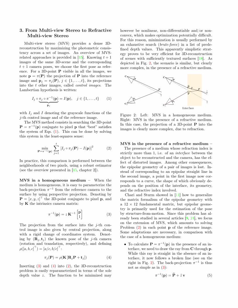
Many Natural History Museums have collections offragile specimens embedded in a transparent medium,for instance a prehistoric insect trapped in a block ofamber, or a small animal conserved in a solution offormaldehyde or alcohol in a glass jar (see Fig. 1). Theyconstitute an invaluable source of information for evo-lutionary scientists.

Figure 1: Prehistoric beetle trapped in amber (seenunder a microscope), and reptiles specimens in jars,from the Natural History Museum in Copenhagen.

Exploitation of these resources necessitates “seethrough” 3D-estimation techniques. Computerised to-mography (CT) provides a 3D-reconstruction, howeverit requires special CT scanners that can handle objectsof various sizes. It is expensive and time consuming.This may be feasible for a limited amount of samplesbut out of reach for large collections (thousands of am-ber pieces, or linear kilometers of specimens in jars).Photogrammetric 3D-scanning is a reasonable alterna-tive, which however requires overcoming several diffi-culties.

First of all, if the refractive medium deflects the tra-jectory of light rays that pass through it, the shape ofthe interface, i.e. the separation surface between airand this medium, has a strong influence on the appear-ance of the object to be reconstructed. In the exampleon the left in Fig. 1, it is not forbidden to cut the am-ber block to give it a particular shape, as long as thisdoes not alter the insect. The shape of the refractiveinterface will thus be assumed to be known. However,unlike most existing techniques, we do not restrict ourattention to the planar case.

Refraction can cause other difficulties. Because itis wavelength dependent, it causes light dispersion.In addition, an inhomogeneous transparent mediummay have spatially varying refractive index, resultingin light rays that are not straight. Taking a varyingrefractive index into account does not present an in-tractable difficulty, but estimating this index at eachpoint in the medium is in itself a difficult problem. Wewill therefore assume that the refractive medium is ho-mogeneous and that the refractive index varies littlewith wavelength.

1

Contributions – We introduce a general 3D-reconstruction method for objects trapped inside a ho-mogeneous refractive medium with arbitrary, knowninterface, from a set of calibrated multi-view stereo im-ages. The paper is organized as follows. In Section 2,we review the main studies taking into account refrac-tion. We show in Section 3 how to extend the multi-view stereo technique in the presence of an interface.The main difficulty of this extension, which is detailedin Section 4, consists in predicting the projection in animage of a 3D point located in the refractive medium.A first set of tests is conducted in Section 5 to validatethis method. In Section 6, we show how to extend it toany shape of the interface. Section 7 allows us to vali-date it on real data. Finally, we conclude in Section 8by mentioning some possible extensions.

2. State of the Art

Light rays from a point source naturally tend todiverge. By refraction, a lens allows to deviate theirtrajectories to make them converge in an image point.Refraction is therefore the key to optical instruments,with the caveat that manufacturing a photographic lensassembly requires very precise alignment of the lensesthat make it up, in order to limit undesired effects,called aberrations. However, if the scene itself containstransparent, i.e. refractive, objects, this modifies theappearance of opaque objects, which appear distorted.

Correcting refraction in the images – A numberof papers have addressed the correction of these distor-tions when the transparent object, such as a windowpane, is attached to the front of the camera, in whichcase the distortions can be calibrated, and standard3D-reconstruction pipelines can then be employed. Forexample, while it is relevant to use photogrammetry tostudy convection in a water-filled tank, Maas showsin [28] how to take into account refraction throughboth sides of the glass to improve measurement ac-curacy. In [27], Luczynski et al. show how to correctthe images acquired by a pair of calibrated underwatercameras, protected by a glass plate, to restore epipolargeometry. The same idea of pre-correcting the imageshas also been explored in [1, 34], as well as in [2] wherecorrection is carried out by neural networks. It has alsobeen shown in [20, 37] that light field cameras can pro-vide useful clues for correcting refraction in the images.Another example where the consideration of refractionis required is the 3D-reconstruction of the seabed fromaerial images [7, 30].

Active refraction techniques – On the otherhand, several studies, which can be grouped under the

term active refraction, take advantage of refraction toallow 3D-reconstruction from a single view, thanks toimage duplication, using either a bi-prism [25, 35], or aglass plate rotating around the optical axis [12, 17]. Aproblem involving refraction, but with a different goalthan ours, is that of estimating the surface of a trans-parent object. The solution proposed by Morris andKutulakos consists in mapping points of interest seenthrough transparency [29]. Another approach is thatof Ben-Ezra and Nayar [6], who fit the parameters of asurface model in order to reproduce the distorted imageof an object of known geometry. The 3D-reconstructionof transparent objects has also been revisited recentlyunder the neural network perspective [26].

Refractive structure-from-motion – Chari andSturm showed in [11] how to extend epipolar geometryin the case where the camera is separated from the 3D-scene by a planar interface, using a 12×12 fundamentalmatrix. The explicit consideration of refraction in theestimation of pose by structure-from-motion was alsostudied by Jordt et al. [21, 22], Kang et al. [23], Qiao etal. [31], Suresh et al. [32], and most recently by Chade-becq et al. [9]. In most of these papers, validation iscarried out on underwater images – a recent survey ofunderwater 3D-imaging techniques can be found in [8].

Refractive multi-view stereo – In this pa-per, we rather assume that the camera poses havebeen pre-calibrated, e.g. by structure-from-motion,and we focus on 3D-reconstruction by multi-viewstereo (MVS). Extensions of the PMVS algorithm(patch-based multi-view stereo) by Furukawa andPonce [16] have been proposed by Kang et al. [24]and by Chang and Chen [10], but the extensionprocess is not really detailed. Agrawal et al. havealso studied MVS in a refractive medium in [3], buttheir work remains limited to a (multi-layer) planarinterface. To the best of our knowledge, the onlywork considering a non-planar interface is the recentwork of Yoon et al. [36]. However, their objectiveis different, because the curved refractive medium isplaced between the observer and the object, whilein our case the object lies inside the refractive medium.

Overall, there is a lack of multi-view stereo methodadapted to the case of an object placed in a refractivemedium with non-planar shape. The goal of our workis to fill this gap.

3. From Multi-view Stereo to RefractiveMulti-view Stereo

Multi-view stereo (MVS) provides a dense 3D-reconstruction by maximizing the photometric consis-tency across a set of images. An overview of MVS-related approaches is provided in [15]. Knowing t + 1images of the same 3D-scene and the correspondingt + 1 camera poses, we choose the first pose as refer-ence. For a 3D-point P visible in all the images, wenote p = π(P) the projection of P into the referenceimage and pj = πj(P), j ∈ {1, . . . , t}, its projectionsinto the t other images, called control images. TheLambertian hypothesis is written:

Ij ◦ πj ◦ π−1(p)︸ ︷︷ ︸pj

= I(p), j ∈ {1, . . . , t} (1)

with Ij and I denoting the grayscale functions of thej-th control image and of the reference image.

The MVS method consists in searching the 3D-pointP = π−1(p) conjugate to pixel p that “best” satisfiesthe system of Eqs. (1). This can be done by solvingthis system in the least-squares sense:

minP=π−1(p)

t∑j=1

[Ij ◦ πj(P)− I(p)]2 (2)

In practice, this comparison is performed between theneighborhoods of two pixels, using a robust estimator(see the overview presented in [15, chapter 2]).

MVS in a homogeneous medium – When themedium is homogeneous, it is easy to parameterize theback-projection π−1 from the reference camera to thesurface by using perspective projection. Denoting byP = [x, y, z]> the 3D-point conjugate to pixel p, andby K the intrinsics camera matrix:

π−1(p) = zK−1[p1

](3)

The projection from the surface into the j-th con-trol image is also given by central projection, alongwith a rigid change of coordinates system. Denot-ing by (Rj , tj) the known pose of the j-th camera(rotation and translation, respectively), and definingρ([a, b, c]

>) = [a/c, b/c]

>:

πj(P) = ρ(K [RjP + tj ]) (4)

Inserting (3) and (4) into (2), the 3D-reconstructionproblem is easily reparameterized in terms of the soledepth value z. The function to be minimized may

however be nonlinear, non-differentiable and/or non-convex, which makes optimization potentially difficult.For this reason, minimization is usually performed byan exhaustive search (brute-force) in a list of prede-fined depth values. This apparently simplistic strat-egy proves to be very efficient for 3D-reconstructionof scenes with sufficiently textured surfaces [18]. Asdepicted in Fig. 2, the scenario is similar, but clearlymore complex, in the presence of a refractive medium.

Figure 2: Left: MVS in a homogeneous medium.Right: MVS in the presence of a refractive medium.In this case, the projection of a 3D-point P into theimages is clearly more complex, due to refraction.

MVS in the presence of a refractive medium –The presence of a medium whose refraction index is

strictly more than 1, i.e. of an interface between theobject to be reconstructed and the camera, has the ef-fect of distorted images. Among other consequences,the epipolar geometry of a pair of images is lost. In-stead of corresponding to an epipolar straight line inthe second image, a point in the first image now cor-responds to a curve, the shape of which obviously de-pends on the position of the interface, its geometry,and the refractive index involved.

Chari and Sturm showed in [11] how to generalizethe matrix formalism of the epipolar geometry witha 12 × 12 fundamental matrix, but epipolar geome-try is primarily used for the estimation of the poseby structure-from-motion. Since this problem has al-ready been studied in several articles [9, 21], we focuson the extension of MVS, which amounts to solvingProblem (2) in each point p of the reference image.Some adaptations are necessary, in comparison withthe case of a homogeneous medium:

• To calculate P = π−1(p) in the presence of an in-terface, we need to draw the ray fromC through p.While this ray is straight in the absence of an in-terface, it now follows a broken line (see on theright in Fig. 2). The back-projection π−1 is thusnot as simple as in (3):

π−1(p) = P + z v (5)

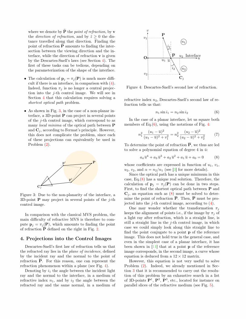
where we denote by P the point of refraction, by vthe direction of refraction, and by z ≥ 0 the dis-tance travelled along that direction. Finding thepoint of refraction P amounts to finding the inter-section between the viewing direction and the in-terface, while the direction of refraction v is givenby the Descartes-Snell’s laws (see Section 4). Thefirst of these tasks can be tedious, depending onthe parameterization of the shape of the interface.

• The calculation of pj = πj(P) is much more diffi-cult if there is an interface, in comparison with (4).Indeed, function πj is no longer a central projec-tion into the j-th control image. We will see inSection 4 that this calculation requires solving ashortest optical path problem.

• As shown in Fig. 3, in the case of a non-planar in-terface, a 3D-point P can project in several pointsof the j-th control image, which correspond to asmany local minima of the optical path between Pand Cj , according to Fermat’s principle. However,this does not complicate the problem, since eachof these projections can equivalently be used inProblem (2).

Figure 3: Due to the non-planarity of the interface, a3D-point P may project in several points of the j-thcontrol image.

In comparison with the classical MVS problem, themain difficulty of refractive MVS is therefore to com-pute pj = πj(P), which amounts to finding the pointof refraction P defined on the right in Fig. 2.

4. Projections into the Control Images

Descartes-Snell’s first law of refraction tells us thatthe refracted ray lies in the plane of incidence, definedby the incident ray and the normal to the point ofrefraction P. For this reason, one can represent therefraction phenomenon within a plane (see Fig. 4).

Denoting by i1 the angle between the incident lightray and the normal to the interface, in a medium ofrefractive index n1, and by i2 the angle between therefracted ray and the same normal, in a medium of

O u

vP

Cj

v1

v2

u1u2

u

P

i1

i2

Interface

n1

n2

Figure 4: Descartes-Snell’s second law of refraction.

refractive index n2, Descartes-Snell’s second law of re-fraction tells us that:

n1 sin i1 = n2 sin i2 (6)

In the case of a planar interface, let us square bothmembers of Eq.(6), using the notations of Fig. 4:

n21(u1 − u)2

(u1 − u)2 + v21= n22

(u2 − u)2

(u2 − u)2 + v22(7)

To determine the point of refraction P, we thus are ledto solve a polynomial equation of degree 4 in u:

a4 u4 + a3 u

3 + a2 u2 + a1 u+ a0 = 0 (8)

whose coefficients are expressed in function of u1, v1,u2, v2, and α = n2/n1 (see [3] for more details).

Since the optical path has a unique minimum in thiscase, Eq.(8) has a unique real solution. Therefore, thecalculation of pj = πj(P) can be done in two steps.First, to find the shortest optical path between P andCj , an equation such as (8) must be solved to deter-mine the point of refraction P. Then, P must be pro-jected into the j-th control image, according to (4).

One may wonder whether the transformation πjkeeps the alignment of points i.e., if the image by πj ofa light ray after refraction, which is a straight line, isstill a straight line in the j-th control image, in whichcase we could simply look along this straight line tofind the point conjugate to a point p of the referenceimage. This does not hold true in the general case, andeven in the simplest case of a planar interface, it hasbeen shown in [11] that at a point p of the referenceimage corresponds, in the second image, a curve whoseequation is deduced from a 12× 12 matrix.

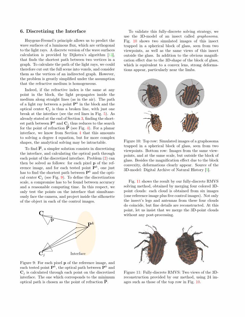
However, this equation is not very useful to solveProblem (2). Indeed, we already mentioned in Sec-tion 3 that it is recommended to carry out the resolu-tion of this problem by an exhaustive search in a listof 3D-points P1, P2, P3, etc., located for instance onparallel slices of the refractive medium (see Fig. 5).

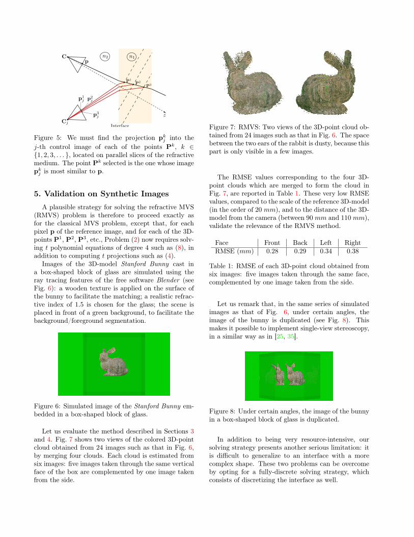
Figure 5: We must find the projection pkj into thej-th control image of each of the points Pk, k ∈{1, 2, 3, . . . }, located on parallel slices of the refractivemedium. The point Pk selected is the one whose imagepkj is most similar to p.

5. Validation on Synthetic Images

A plausible strategy for solving the refractive MVS(RMVS) problem is therefore to proceed exactly asfor the classical MVS problem, except that, for eachpixel p of the reference image, and for each of the 3D-points P1, P2, P3, etc., Problem (2) now requires solv-ing t polynomial equations of degree 4 such as (8), inaddition to computing t projections such as (4).

Images of the 3D-model Stanford Bunny cast ina box-shaped block of glass are simulated using theray tracing features of the free software Blender (seeFig. 6): a wooden texture is applied on the surface ofthe bunny to facilitate the matching; a realistic refrac-tive index of 1.5 is chosen for the glass; the scene isplaced in front of a green background, to facilitate thebackground/foreground segmentation.

Figure 6: Simulated image of the Stanford Bunny em-bedded in a box-shaped block of glass.

Let us evaluate the method described in Sections 3and 4. Fig. 7 shows two views of the colored 3D-pointcloud obtained from 24 images such as that in Fig. 6,by merging four clouds. Each cloud is estimated fromsix images: five images taken through the same verticalface of the box are complemented by one image takenfrom the side.

Figure 7: RMVS: Two views of the 3D-point cloud ob-tained from 24 images such as that in Fig. 6. The spacebetween the two ears of the rabbit is dusty, because thispart is only visible in a few images.

The RMSE values corresponding to the four 3D-point clouds which are merged to form the cloud inFig. 7, are reported in Table 1. These very low RMSEvalues, compared to the scale of the reference 3D-model(in the order of 20 mm), and to the distance of the 3D-model from the camera (between 90 mm and 110 mm),validate the relevance of the RMVS method.

Face Front Back Left RightRMSE (mm) 0.28 0.29 0.34 0.38

Table 1: RMSE of each 3D-point cloud obtained fromsix images: five images taken through the same face,complemented by one image taken from the side.

Let us remark that, in the same series of simulatedimages as that of Fig. 6, under certain angles, theimage of the bunny is duplicated (see Fig. 8). Thismakes it possible to implement single-view stereoscopy,in a similar way as in [25, 35].

Figure 8: Under certain angles, the image of the bunnyin a box-shaped block of glass is duplicated.

In addition to being very resource-intensive, oursolving strategy presents another serious limitation: itis difficult to generalize to an interface with a morecomplex shape. These two problems can be overcomeby opting for a fully-discrete solving strategy, whichconsists of discretizing the interface as well.

6. Discretizing the Interface

Huygens-Fresnel’s principle allows us to predict thewave surfaces of a luminous flux, which are orthogonalto the light rays. A discrete version of the wave surfacescalculation is provided by Dijkstra’s algorithm [13],that finds the shortest path between two vertices in agraph. To calculate the path of the light rays, we couldtherefore cut out the full scene into voxels, and considerthem as the vertices of an indirected graph. However,the problem is greatly simplified under the assumptionthat the refractive medium is homogeneous.

Indeed, if the refractive index is the same at anypoint in the block, the light propagates inside themedium along straight lines (as in the air). The pathof a light ray between a point Pk in the block and theoptical center Cj is thus a broken line, with just onebreak at the interface (see the red lines in Fig. 5). Asalready stated at the end of Section 3, finding the short-est path between Pk and Cj thus reduces to the searchfor the point of refraction P (see Fig. 4). For a planarinterface, we know from Section 4 that this amountsto solving a degree 4 equation, but for more complexshapes, the analytical solving may be intractable.

To find P, a simpler solution consists in discretizingthe interface, and calculating the optical path througheach point of the discretized interface. Problem (2) canthen be solved as follows: for each pixel p of the ref-erence image, and for each tested point Pk, one justhas to find the shortest path between Pk and the opti-cal center Cj (see Fig. 9). To define the discretizationscale, a compromise has to be found between accuracyand a reasonable computing time. In this respect, weonly test the points on the interface that simultane-ously face the camera, and project inside the silhouetteof the object in each of the control images.

Figure 9: For each pixel p of the reference image, andeach tested point Pk, the optical path between Pk andCj is calculated through each point on the discretizedinterface. The one which corresponds to the minimumoptical path is chosen as the point of refraction P.

To validate this fully-discrete solving strategy, weuse the 3D-model of an insect called graphosoma.Fig. 10 shows two simulated images of this insecttrapped in a spherical block of glass, seen from twoviewpoints, as well as the same views of this insectoutside the glass. In addition to the obvious magnifi-cation effect due to the 3D-shape of the block of glass,which is equivalent to a convex lens, strong deforma-tions appear, particularly near the limbs.

Figure 10: Top row: Simulated images of a graphosomatrapped in a spherical block of glass, seen from twoviewpoints. Bottom row: Images from the same view-points, and at the same scale, but outside the block ofglass. Besides the magnification effect due to the blockconvexity, deformations clearly appear. Source of the3D-model: Digital Archive of Natural History [5].

Fig. 11 shows the result by our fully-discrete RMVSsolving method, obtained by merging four colored 3D-point clouds: each cloud is obtained from six images(one reference image plus five control images). Not onlythe insect’s legs and antennas from these four cloudsdo coincide, but fine details are reconstructed. At thispoint, let us insist that we merge the 3D-point cloudswithout any post-processing.

Figure 11: Fully-discrete RMVS: Two views of the 3D-reconstruction provided by our method, using 24 im-ages such as those of the top row in Fig. 10.

The result in Fig. 11 validates our fully-discreteRMVS solving strategy, at least qualitatively. To con-firm this assertion, Table 2 lists the RMSE values ofthe four 3D-point clouds, to be compared to the scaleof the reference 3D-model (around 20 mm), and to thedistance of the 3D-model from the camera (between90 mm and 110 mm). Without taking refraction intoaccount, the legs and antennas are duplicated (the ab-sence of post-processing accentuates the duplication ef-fect), as shows the result on the left in Fig. 12, whichis confirmed by the RMSE values listed in Table 2.

RMVS (mm) 0.22 0.23 0.18 0.16MVS (mm) 0.51 0.83 0.72 0.31

Table 2: RMSE of each of the 3D-point clouds which,by merging, provide the 3D-reconstruction in Fig. 11(RMVS) and that on the left in Fig. 12 (simple MVS).

As the result on the left in Fig. 12 is obtained by(wrongly) setting the index of the refractive mediumto 1, this shows how crucial a precise knowledge of therefractive index is. An additional result provided byAliceVision, which is a classical SfM/MVS free soft-ware [4], however not intended to consider refraction,is shown on the right in Fig. 12. Unsurprisingly, thisresult is far from being satisfactory, even qualitatively.

Figure 12: Left: Ghost legs and antennas appear whenan erroneous value of the refractive index (here equalto 1) is used. Right: Misunderstanding of the grapho-soma 3D-shape by the AliceVision free software [4].

The image of a straight rod passing through a re-fractive ellipsoid (see Fig. 13) shows to which extentsuch an interface can distort the image. Since the pro-jections of the 3D-points inside the ellipsoid are verydifficult to predict, our fully-discrete RMVS solvingmethod could be less accurate in such a case.

Indeed, Fig. 14 shows how distorted the bunny’simages are, when the glass block is ellipsoidal. Evenif the 3D-reconstruction provided by our fully-discreteRMVS solving method, using six images, is faithful tothe original, it is much less accurate than that of Fig. 7,

Figure 13: Simulated image of a straight rod passingthrough a refractive ellipsoid. The projections of thepoints inside the medium are highlighted in red.

because for some rays, the angle i2 of the Descartes-Snell’s law (6) is very close to π/2 (grazing angle).Since the derivative of the arcsin function tends to-wards infinity in 1, this causes strong inaccuracies inthe calculation of the angle i1 in Eq.(6).

Figure 14: Left: Simulated image of the StanfordBunny inside an ellipsoidal block of glass. Right:Due to the huge distortions of the images, the 3D-reconstruction by RMVS, using six images, is far lessaccurate than that of Fig. 7. However, the generalshape of the reconstructed 3D-point cloud is still muchmore significant of a bunny than the image on the left.

7. Validation on Real Images

Now, let us test this solving method on real images.As sets of images from Natural History Museums havenot yet been produced, we use a present time insectfrom a private collection. It is a grasshopper cast in abox-shaped block of resin. The photographs were takenunder poorly controlled operating conditions, placingthe scene in front of a blue background to facilitatesegmentation (see Fig. 15).

The main difficulty in implementing our 3D-reconstruction method is to estimate the camera poses.We could have used a method of estimation of thepose by refractive structure-from-motion [9], but wealso need to know the position of the faces of the resinblock. So we simply glued a small grid on each face,which allowed us to obtain estimates that were consis-tent with each other.

Figure 15: Two real images of a grasshopper cast ina box-shaped block of resin. The small grid glued oneach side allows us to estimate the camera pose andthe position of the planar interface.

Fig. 16 shows two views of the 3D-reconstructionof the grasshopper obtained from five images takenthrough the same face, plus one image taken from theside (we set the resin refraction index to the plausi-ble value n1 = 1.6). Although imperfect, this result isencouraging. In particular, the reconstructed legs andantennas seem realistic, which is probably an impor-tant criterion in determining whether or not we meetthe needs of entomologists.

Figure 16: 3D-reconstruction of the grasshoper byRMVS: Two views of the 3D-point cloud obtained fromfive images through the same face, plus one side shot.

8. Conclusion and Perspectives

In this paper, we have shown how to adapt the multi-view stereo technique to the case where the object of in-terest is trapped in a refractive medium. Knowing thatrefraction distorts the images, it is necessary to take itinto account to model the path of the light rays. Morespecifically, we have proposed a fully-discrete solvingmethod. Our first results on real data are encouraging,

although there are still many obstacles to overcomebefore this preliminary study leads to an operationalmethod that can be used by entomologists.

Among the tasks to be carried out as a priority, itis necessary to improve the estimation of the cameraposes, using refractive structure-from-motion methods,which are based on the matching between points of in-terest seen by transparency, provided that the epipolargeometry is adapted [11].

Another improvement of our method will consist inestimating the block 3D-shape, resorting for instance toshape-from-silhouettes [19]. By taking care to place theblock in front of a colored background, as we alreadydid (see Fig. 15), this technique allows one to estimatethe volume of any convex object, provided a sufficientnumber of images are used.

As already noticed, another essential characteris-tic of the refractive medium, whose precise estimationwould improve the results on real data, is its index,which was arbitrarily set at 1.6 for the test in Fig. 16.Recall that the problem would be much more complexif the refractive index of the material were not homo-geneous.

The efficiency of our RMVS solving method couldalso be improved. To give an order of magnitude ofthe complexity of this resolution strategy, each 3D-point cloud giving, by merging, the result on the leftof Fig. 7, is obtained with t = 5 control images. Thereference image has about 1.5×105 pixels. Since theblock of glass is discretized into 200 slices, the com-plete resolution of Problem (2) requires solving about108 equations of degree 4, which takes about one hourof computing time on a standard PC, using either ananalytical or a bisection method of solving.

Finally, in the longer term, we plan to adapt torefraction the photometric 3D-reconstruction meth-ods that are shape-from-shading [14] and photometricstereo [33]. To our knowledge, these problems havebeen very rarely addressed in the refractive case. Inaddition to the need to model the phenomenon of lightattenuation inside the refractive medium, according toBeer-Lambert’s law, it will also be necessary to takecolor into account, i.e. to consider that this attenua-tion depends on the wavelength. And while we havedeliberately ignored light scattering, this phenomenonwill also have to be taken into account in the contextof photometric 3D-reconstruction.

References[1] P. Agrafiotis, K. Karantzalos, A. Georgopoulos, and

D. Skarlatos. Correcting image refraction: Towardsaccurate aerial image-based bathymetry mapping inshallow waters. Remote Sensing, 12(2):322, 2020. 2

[2] P. Agrafiotis, D. Skarlatos, A. Georgopoulos, andK. Karantzalos. DepthLearn: learning to correct therefraction on point clouds derived from aerial imageryfor accurate dense shallow water bathymetry based onSVMs-fusion with LiDAR point clouds. Remote Sens-ing, 11(19):2225, 2019. 2

[3] A. Agrawal, S. Ramalingam, Y. Taguchi, and V. Chari.A theory of multi-layer flat refractive geometry. In Pro-ceedings of the IEEE Conference on Computer Visionand Pattern Recognition, pages 3346–3353, 2012. 2, 4

[4] AliceVision. https://alicevision.org/. 7[5] Digital Archive of Natural History. https://

sketchfab.com/disc3d. 6[6] M. Ben-Ezra and S. K. Nayar. What does motion

reveal about transparency? In Proceedings of theIEEE International Conference on Computer Vision,volume 2, pages 1025–1032, 2003. 2

[7] B. Cao, R. Deng, and S. Zhu. Universal algorithmfor water depth refraction correction in through-waterstereo remote sensing. International Journal of AppliedEarth Observation and Geoinformation, 91:102108,2020. 2

[8] M. Castillón, A. Palomer, J. Forest, and P. Ridao.State of the Art of Underwater Active Optical 3DScanners. Sensors, 19(23):5161, 2019. 2

[9] F. Chadebecq, F. Vasconcelos, R. Lacher, E. Maneas,A. Desjardins, S. Ourselin, T. Vercauteren, andD. Stoyanov. Refractive Two-View Reconstruction forUnderwater 3D Vision. International Journal of Com-puter Vision, 128:1101–1117, 2020. 2, 3, 7

[10] Y. J. Chang and T. Chen. Multi-View 3D Reconstruc-tion for Scenes under the Refractive Plane with KnownVertical Direction. In Proceedings of the IEEE Interna-tional Conference on Computer Vision, pages 351–358,2011. 2

[11] V. Chari and P. Sturm. Multiple-View Geometry ofthe Refractive Plane. In Proceedings of the BritishMachine Vision Conference, pages 1–11, 2009. 2, 3,4, 8

[12] Z. Chen, K.-Y. K. Wong, Y. Matsushita, and X. Zhu.Depth from refraction using a transparent mediumwith unknown pose and refractive index. InternationalJournal of Computer Vision, 102(1–3):3–17, 2013. 2

[13] E. W. Dijkstra. A note on two problems in connex-ion with graphs. Numerische Mathematik, 1:269–271,1959. 6

[14] J.-D. Durou, M. Falcone, and M. Sagona. Numeri-cal Methods for Shape-from-shading: A New Surveywith Benchmarks. Computer Vision and Image Un-derstanding, 109(1):22–43, 2008. 8

[15] Y. Furukawa and C. Hernàndez. Multi-View Stereo: ATutorial. Foundations and Trends in Computer Graph-ics and Vision, 9(1–2):1–148, 2015. 3

[16] Y. Furukawa and J. Ponce. Accurate, Dense, and Ro-bust Multiview Stereopsis. IEEE Transactions on Pat-tern Analysis and Machine Intelligence, 32(8):1362–1376, 2010. 2

[17] C. Gao and N. Ahuja. A Refractive Camera for Ac-quiring Stereo and Super-resolution Images. In Pro-ceedings of the IEEE Conference on Computer Visionand Pattern Recognition, pages 2316–2323, 2006. 2

[18] M. Goesele, B. Curless, and S. M. Seitz. Multi-ViewStereo Revisited. In Proceedings of the IEEE Con-ference on Computer Vision and Pattern Recognition,pages 2402–2409, 2006. 3

[19] C. Hernández and F. Schmitt. Silhouette and stereofusion for 3D object modeling. Computer Vision andImage Understanding, 96(3):367–392, 2004. 8

[20] K. Ichimaru and H. Kawasaki. Underwater StereoUsing Refraction-Free Image Synthesized From LightField Camera. In Proceedings of the IEEE Interna-tional Conference on Image Processing, pages 1039–1043, 2019. 2

[21] A. Jordt, K. Köser, and R. Koch. Refractive 3D recon-struction on underwater images. Methods in Oceanog-raphy, 15–16:90–113, 2016. 2, 3

[22] A. Jordt-Sedlazeck, D. Jung, and R. Koch. RefractivePlane Sweep for Underwater Images. In Proceedings ofthe German Conference on Pattern Recognition, pages333–342, 2013. 2

[23] L. Kang, L. Wu, Y. Wei, S. Lao, and Y.-H. Yang.Two-view underwater 3D reconstruction for cameraswith unknown poses under flat refractive interfaces.Pattern Recognition, 69:251–269, 2017. 2

[24] L. Kang, L. Wu, and Y. H. Yang. Two-View Under-water Structure and Motion for Cameras under FlatRefractive Interfaces. In Proceedings of the EuropeanConference on Computer Vision, volume 7575 of Lec-ture Notes in Computer Science, pages 303–316, 2012.2

[25] D. H. Lee, I.-S. Kweon, and R. Cipolla. A biprism-stereo camera system. In Proceedings of the IEEE Con-ference on Computer Vision and Pattern Recognition,volume 1, page 87, 1999. 2, 5

[26] Z. Li, Y.-Y. Yeh, and M. Chandraker. Through theLooking Glass: Neural 3D Reconstruction of Trans-parent Shapes. In Proceedings of the IEEE/CVF Con-ference on Computer Vision and Pattern Recognition,pages 1262–1271, 2020. 2

[27] T. Luczynski, M. Pfingsthorn, and A. Birk. Imagerectification with the pinax camera model in underwa-ter stereo systems with verged cameras. In OCEANS2017, pages 1–7, 2017. 2

[28] H. G. Maas. New developments in multimedia pho-togrammetry. In Optical 3-D Measurement TechniquesIII, 1995. 2

[29] N. J. W. Morris and K. N. Kutulakos. Dynamic Refrac-tion Stereo. IEEE Transactions on Pattern Analysisand Machine Intelligence, 33(8):1518–1531, 2011. 2

[30] T. Murase, M. Tanaka, T. Tani, Y. Miyashita,N. Ohkawa, S. Ishiguro, Y. Suzuki, H. Kayanne, andH. Yamano. A Photogrammetric Correction Proce-dure for Light Refraction Effects at a Two-MediumBoundary. Photogrammetric Engineering and RemoteSensing, 9(8):1129–1136, 2008. 2

[31] X. Qiao, Y. Ji, A. Yamashita, and H. Asama. Structurefrom Motion of Underwater Scenes Considering Im-age Degradation and Refraction. IFAC-PapersOnLine,52(22):78–82, 2019. 2

[32] S. Suresh, E. Westman, and M. Kaess. Through-water stereo slam with refraction correction for AUVlocalization. IEEE Robotics and Automation Letters,4(2):692–699, 2019. 2

[33] R. J. Woodham. Photometric Method For Determin-ing Surface Orientation From Multiple Images. OpticalEngineering, 19(1):134–144, 1980. 8

[34] X. Wu and X. Tang. Accurate binocular stereo under-water measurement method. International Journal ofAdvanced Robotic Systems, 16(5):1729881419864468,2019. 2

[35] A. Yamashita, Y. Shirane, and T. Kaneko. Monocu-lar Underwater Stereo – 3D Measurement Using Dif-ference of Appearance Depending on Optical Paths.In Proceedings of the IEEE/RSJ International Con-ference on Intelligent Robots and Systems, pages 3652–3657, 2010. 2, 5

[36] S. Yoon, T. Choi, and S. Sull. Depth estimation fromstereo cameras through a curved transparent medium.Pattern Recognition Letters, 129:101–107, 2020. 2

[37] C. Zhang, X. Zhang, D. Tu, and P. Jin. On-site cali-bration of underwater stereo vision based on light field.Optics and Lasers in Engineering, 121:252–260, 2019.2