Refinery Operations Presentation-Final2Refinery Operations Planning ... – Calculate blending...
95
Refinery Operations Planning Sarah Kuper Sarah Shobe Andy Hill
Transcript of Refinery Operations Presentation-Final2Refinery Operations Planning ... – Calculate blending...
Refinery Operations Planning
Sarah KuperSarah Shobe
Andy Hill

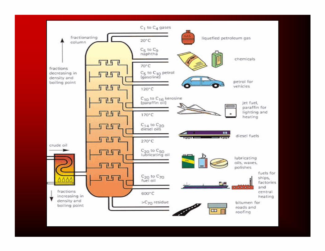
Refinery Operations Planning• What is a refinery?
– Takes crude oil and converts it into gasoline– Distills crude into light, medium, and heavy fractions
• Lightest fractions – gasoline, liquid petroleum gas• Medium fractions – kerosene and diesel oil• Heavy fractions – gas oils and residuum
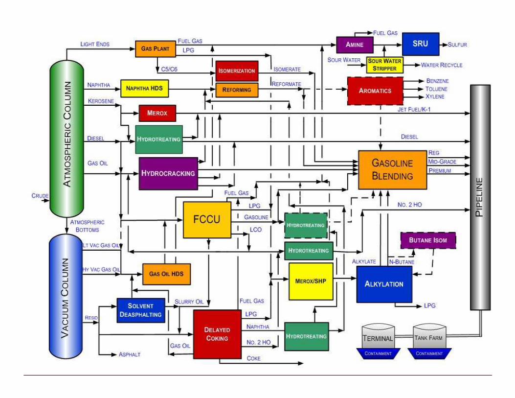

Process that is fed by heavier fractions to produce lighter fractions
Hydrocracker
Reformer
Process used to increase the octane number of light crude fractions
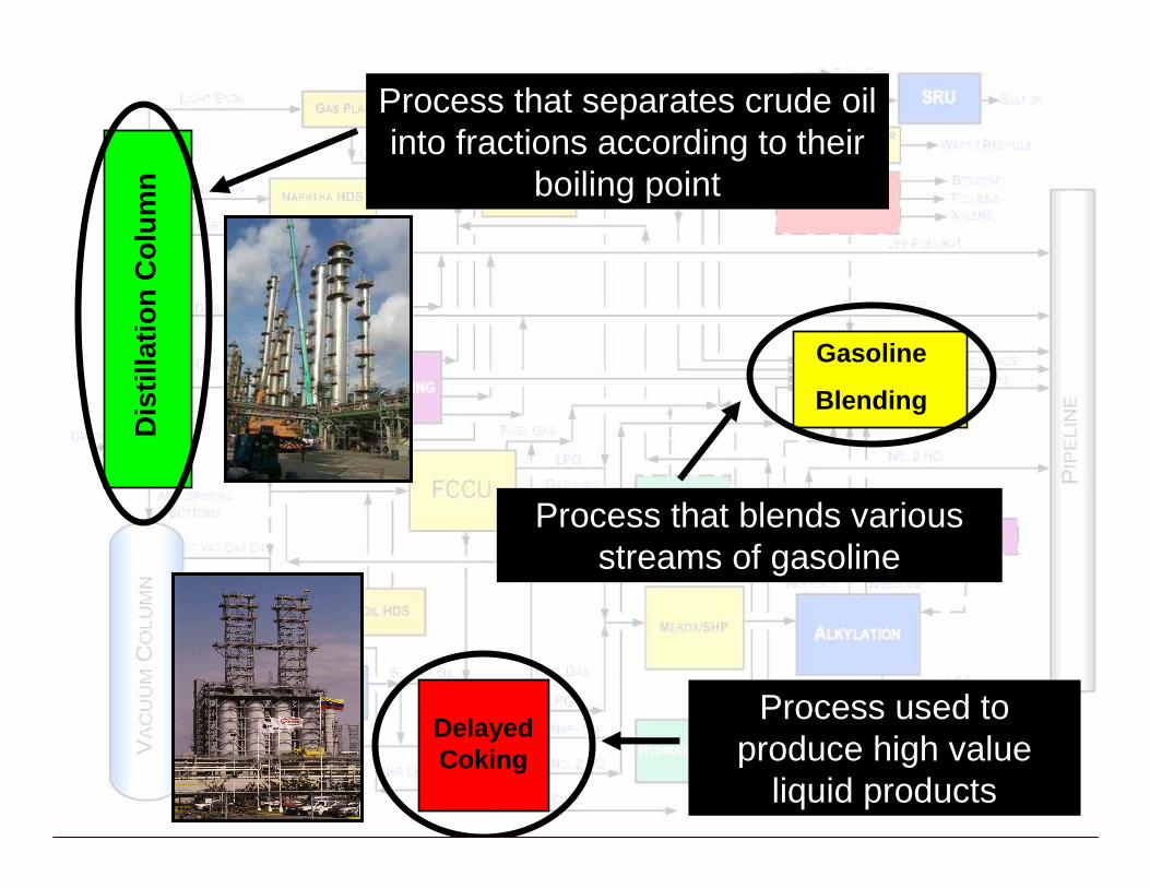
Dis
tilla
tio
n C
olu
mn
Process that separates crude oil into fractions according to their
boiling point
Gasoline
Blending
Process that blends various streams of gasoline
Delayed Coking
Process used to produce high value
liquid products

Hydrotreating
Process that uses H2 to break up sulfur, nitrogen
compounds, and aromatics
Isomerization
Process that converts normal, straight chain
paraffins to iso-paraffins

Refinery Operations Planning
“Refining is a complex operation that depends upon the human skills of operators, engineers, and planners in combination with cutting edge technology to produce the products that meet the demands of an intensely competitive market.”
Sources: http://www.exxon.mobil.com/UK-English/Operations/UK_OP_Ref_RefOp.asp and http://static.flickr.com/18/24007819_4d67ab2c0b.jpg
Refinery Operations Planning
• Planning groups in a refinery attempt to optimize the refinery’s profits by purchasing specific amounts of different crudes
• Based on:– Projected market demands and prices
– Unit capabilities– Planned turnarounds

HDS
FOVS
FO2
GASOLINEPOOL
DIESELPOOL
CDU2
CDU3
MB
FG
LPG Naphtha FO
Kero DO
NPU
LN
HN
ISOU
CRU
HN
FG
REF
LPG
KTU
ISO
LN
Kero
IHSD
MTBET
DCCT
ISOG
SUPG
HSD
JP1
FO1
Products
Intermediates
PHET
SLEB
LB
TP
OM
Crudes
Kero
FO
Kero
Refinery Operations Planning
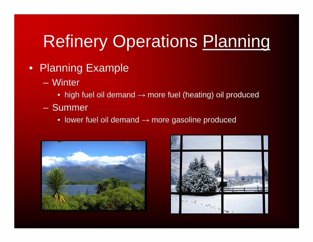
Refinery Operations Planning• Planning Example
– Winter • high fuel oil demand → more fuel (heating) oil produced
– Summer • lower fuel oil demand → more gasoline produced
Refinery Operations Planning
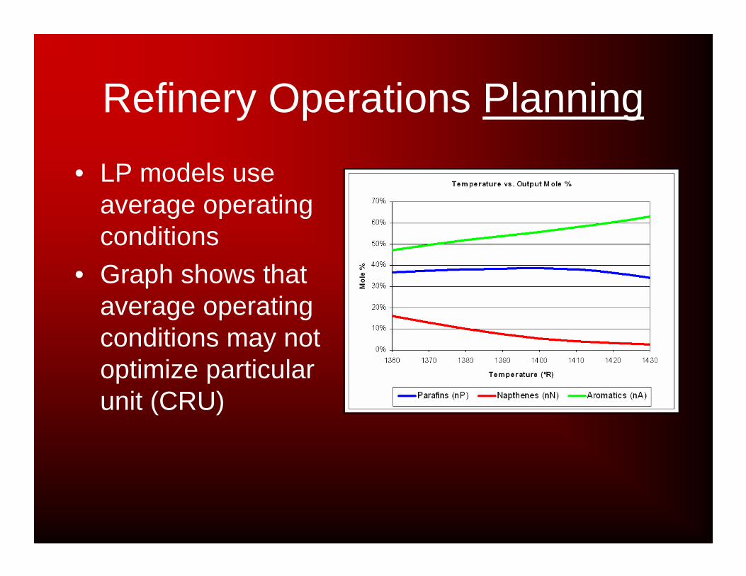
• LP models use average operating conditions
• Graph shows that average operating conditions may not optimize particular unit (CRU)
Current Models
• Current models operate linearly (LP)– Black Box Theory
• PIMS (by Aspentech)• RPMS (by Honeywell Hi-Spec Solutions)• GRMPTS (by Haverly)
HDS
FOVS
FO2
GASOLINEPOOL
DIESELPOOL
CDU2
CDU3
MB
FG
LPG Naphtha FO
Kero DO
NPU
LN
HN
ISOU
CRU
HN
FG
REF
LPG
KTU
ISO
LN
Kero
IHSD
MTBET
DCCT
ISOG
SUPG
HSD
JP1
FO1
Products
Intermediates
PHET
SLEB
LB
TP
OM
Crudes
Kero
FO
Kero
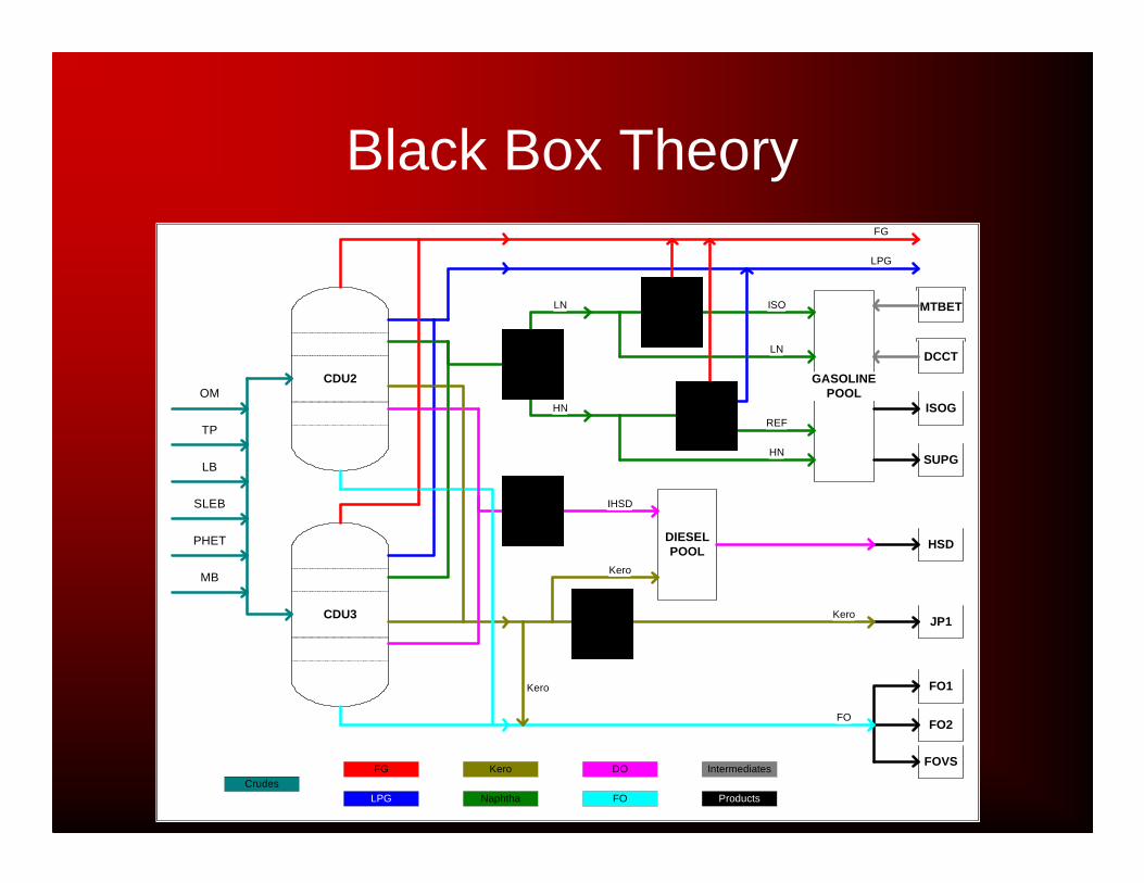
Black Box Theory
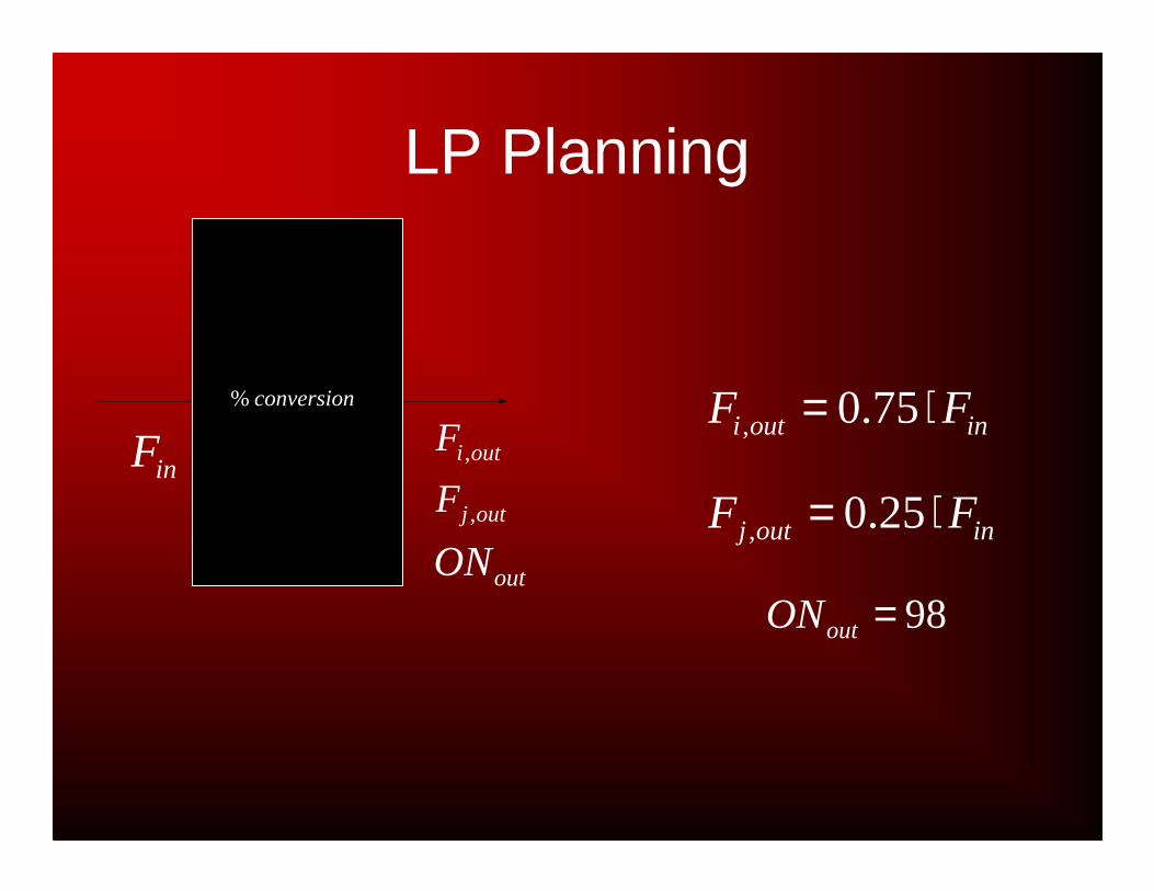
LP Planning
outiF ,inF
conversion%
outON98=outON
inoutj FF ⋅= 25.0,outjF ,
inouti FF ⋅= 75.0,

HDS
FOVS
FO2
GASOLINEPOOL
DIESELPOOL
CDU2
CDU3
MB
FG
LPG Naphtha FO
Kero DO
NPU
LN
HN
ISOU
CRU
HN
FG
REF
LPG
KTU
ISO
LN
Kero
IHSD
MTBET
DCCT
ISOG
SUPG
HSD
JP1
FO1
Products
Intermediates
PHET
SLEB
LB
TP
OM
Crudes
Kero
FO
Kero
Modeling Unit Operations
HDS
Operating Variables:
Temperature
Pressure
Flow Rate
Input Sulfur
Weight Percent

Modeling Unit Operations
HDS
Operating Variables:
Temperature
Pressure
Flow Rate
Input Sulfur
Weight Percent
),,(, FPTfF outS =
inF outHCF ,
[ ]outSoutSF ,

General Goal
• To effectively model a refinery’s unit operations in the overall planning model.
• Bangchak refinery in Thailand is used as a case study.

More Specific Goals
• Model Hydrotreaters
• Model Catalytic Reformers• Model Isomerization
• Tie Unit Operations to GRM– Add Operating Costs
• Tie Unit Operations to blending– Calculate blending properties
• Integrate Fuel Gas system• Create Hydrogen balance
Original LP Model
• LP model developed– Operates using Black Box theory
• Optimizes purchased crudes and additives• Evaluates uncertainty and risk

Bangchak Refinery
HDS
FOVS
FO2
GASOLINEPOOL
DIESELPOOL
CDU2
CDU3
MB
FG
LPG Naphtha FO
Kero DO
NPU
LN
HN
ISOU
CRU
HN
FG
REF
LPG
KTU
ISO
LN
Kero
IHSD
MTBET
DCCT
ISOG
SUPG
HSD
JP1
FO1
Products
Intermediates
PHET
SLEB
LB
TP
OM
Crudes
Kero
FO
Kero
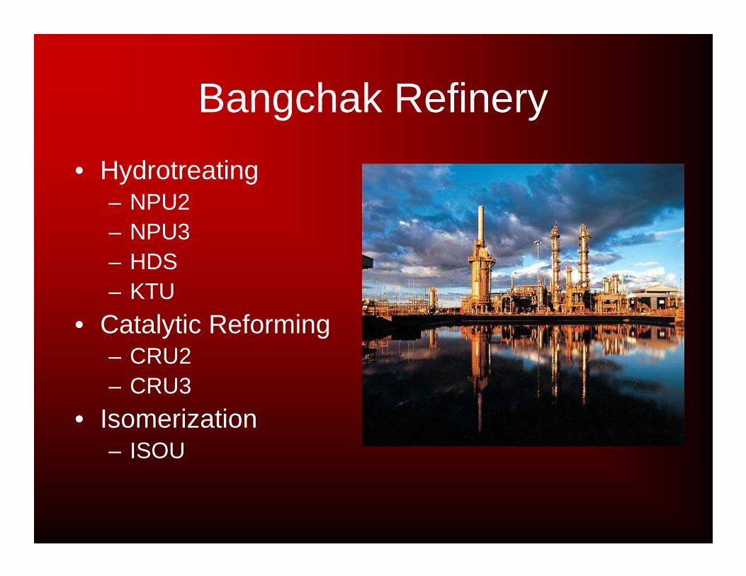
Bangchak Refinery
• Hydrotreating– NPU2– NPU3– HDS– KTU
• Catalytic Reforming– CRU2– CRU3
• Isomerization– ISOU
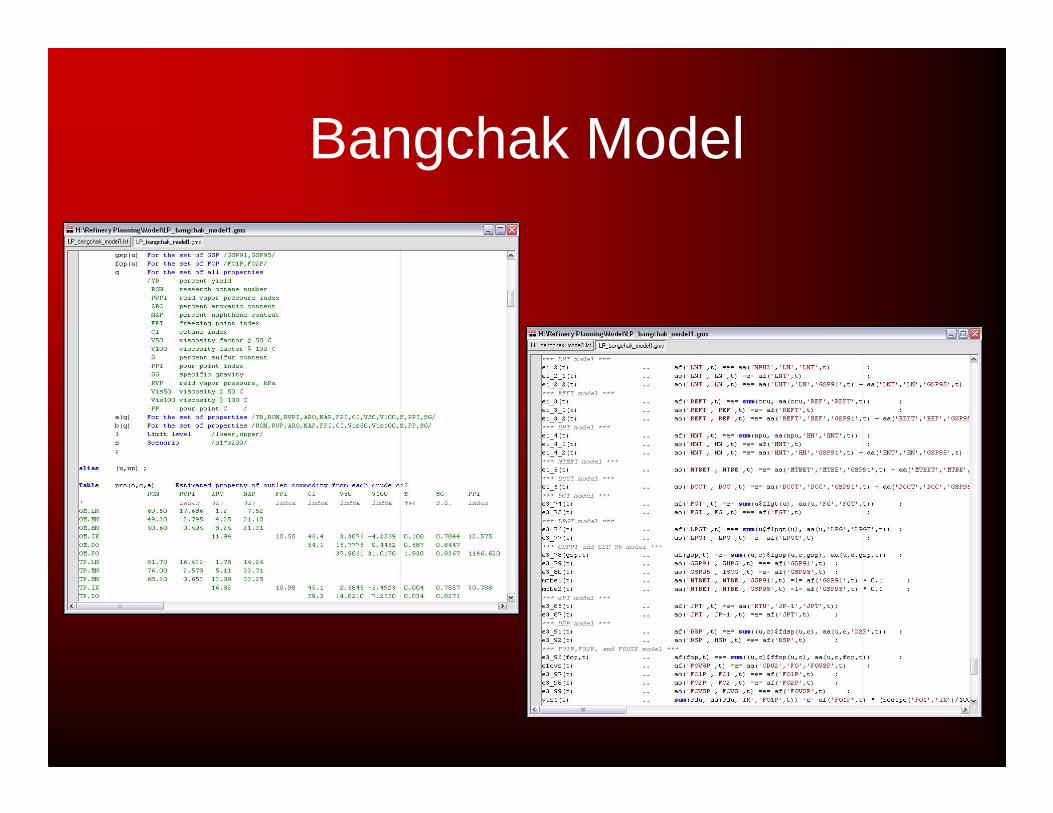
Bangchak Model
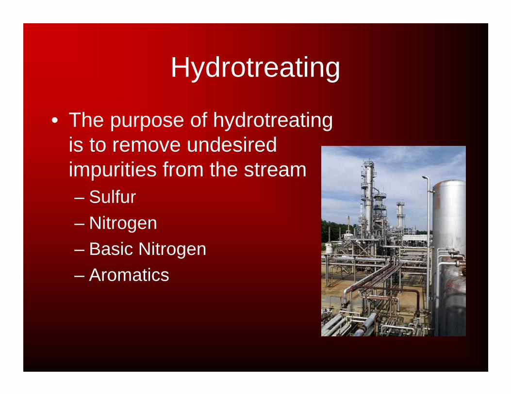
Hydrotreating
• The purpose of hydrotreatingis to remove undesired impurities from the stream– Sulfur
– Nitrogen– Basic Nitrogen– Aromatics

Hydrotreating Reactions
• Most common non-hydrocarbon by-products:– H2S– NH3

Hydrotreating PFD

Hydrotreating Model
• Langmuir-Hinshelwood kinetic rate law
• Main operating variables– Temperature (600-800°C)
– Pressure (100-3000 psig)– H2/HC ratio (2000 ft3/bbl)
– Space Velocity (1.5-9.0)• Based on Flow Rate and Volume

Langmuir-Hinshelwood
( )
⋅+⋅
⋅−= 2
45.0
22
2
1 SHSH
HS
CK
CCkr
Where, k = rate constantKH2S = adsorption equilibrium constant
A = Arrhenius constant
E = activation energy
TR
E
eAk ⋅−
⋅= TRSH eK ⋅⋅=
2761
84.417692
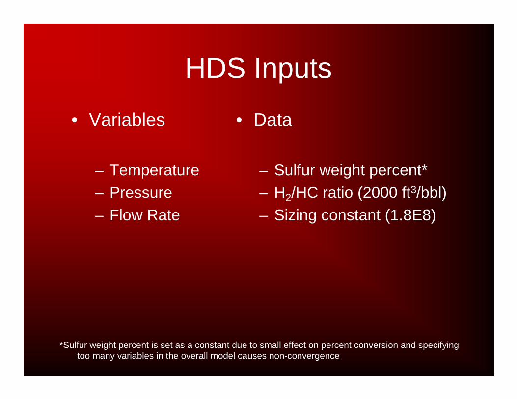
HDS Inputs
• Variables
– Temperature– Pressure– Flow Rate
• Data
– Sulfur weight percent*– H2/HC ratio (2000 ft3/bbl)– Sizing constant (1.8E8)
*Sulfur weight percent is set as a constant due to small effect on percent conversion and specifying too many variables in the overall model causes non-convergence
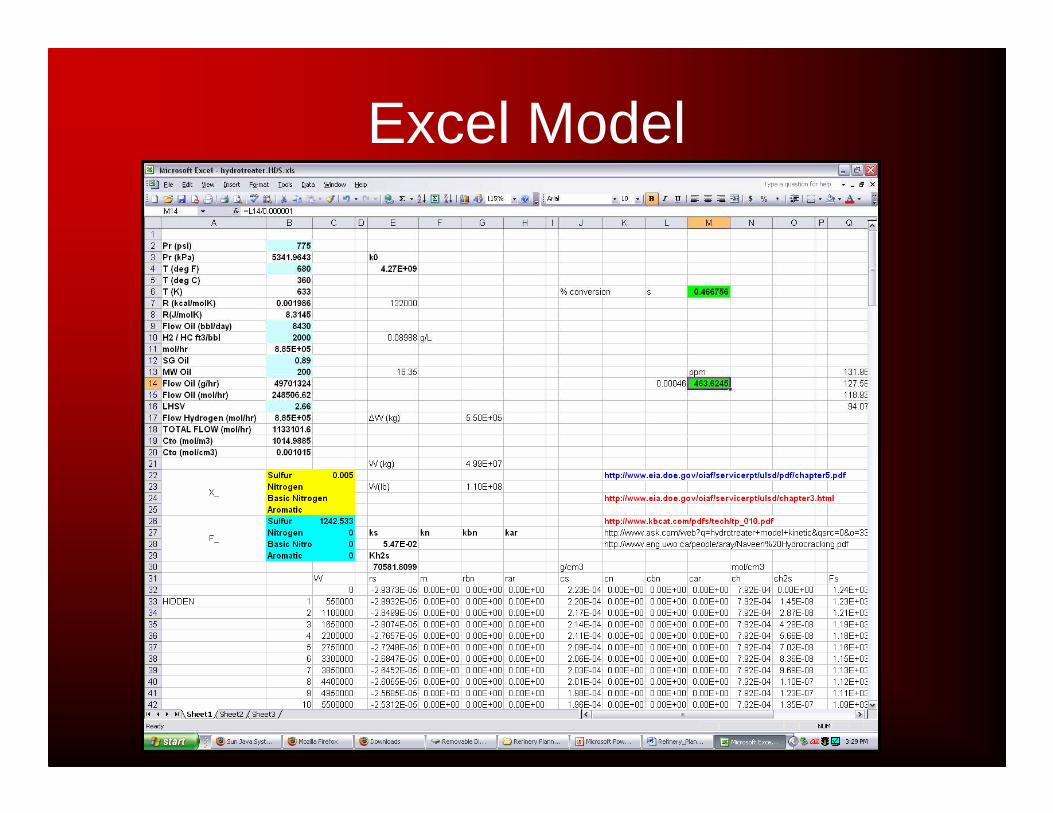
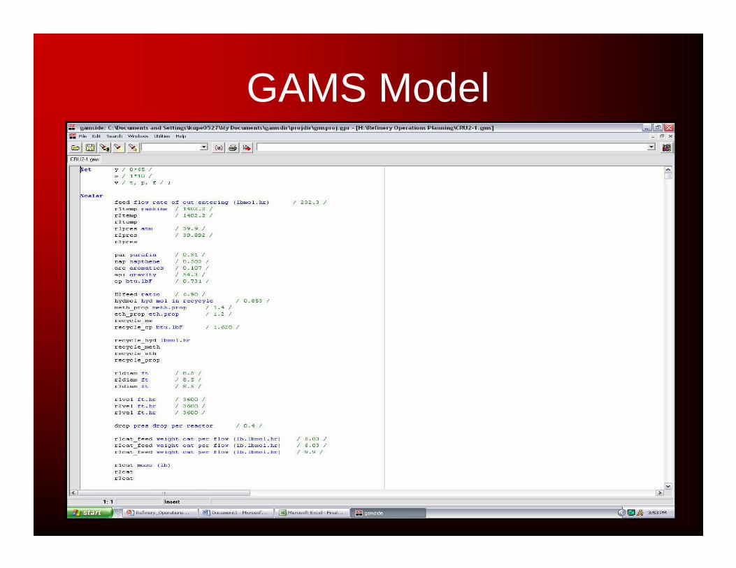
Excel Model

GAMS Model
Catalytic Reforming
• Process used to increase the octane number of light crude fractions
• Converts low-octane naptha into high-octane aromatics
• High octane product is useful for creating premium gasolines
• Hydrogen is the by-product

Catalytic ReformingProcess Flow Diagram
Catalytic Reforming Unit Operating Conditions
• Low pressures (30- 40atm)• High Temperatures (900- 950 ºF)• Feedstock
– Heavy naphtha from hydrotreating unit
• Catalyst – Platinum bi-function catalyst on Alumina
support
• Continuous process– Catalyst is removed, replaced, and
regenerated continuously and online
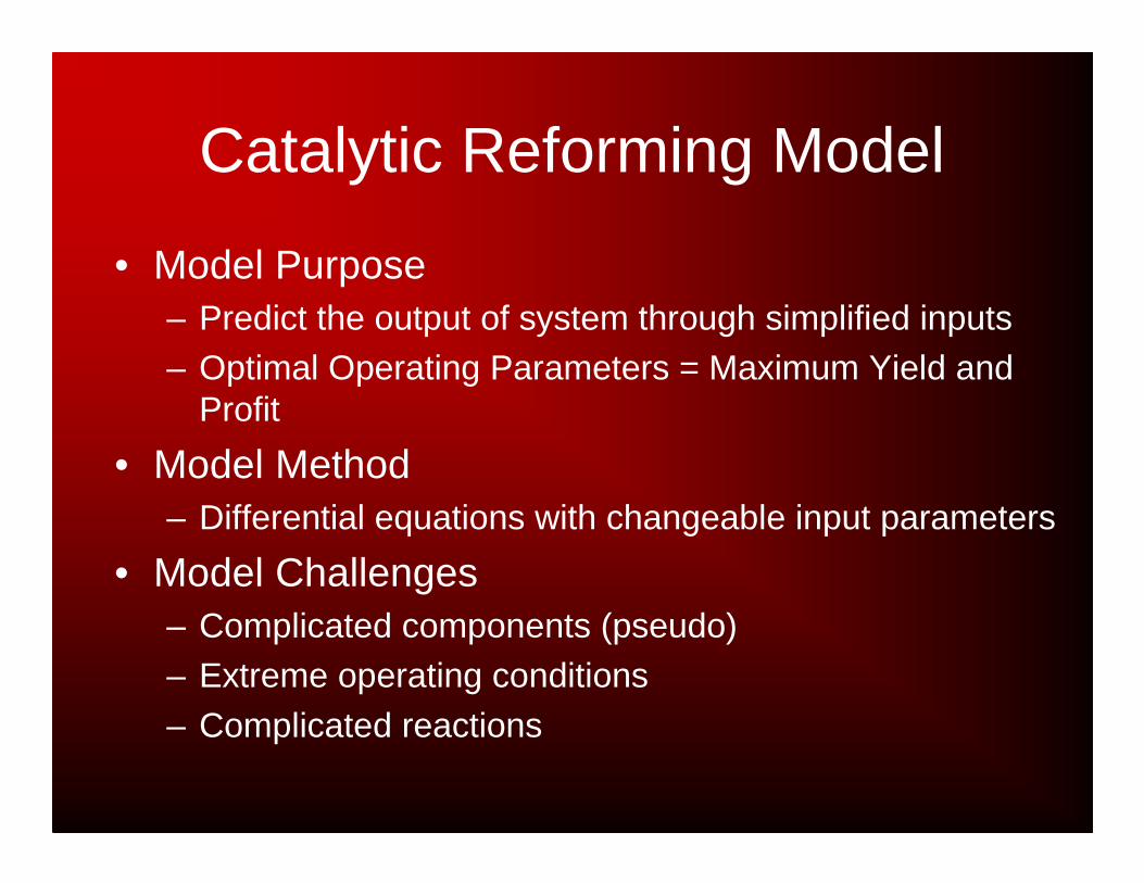
Catalytic Reforming Model
• Model Purpose– Predict the output of system through simplified inputs– Optimal Operating Parameters = Maximum Yield and
Profit
• Model Method– Differential equations with changeable input parameters
• Model Challenges– Complicated components (pseudo)– Extreme operating conditions – Complicated reactions
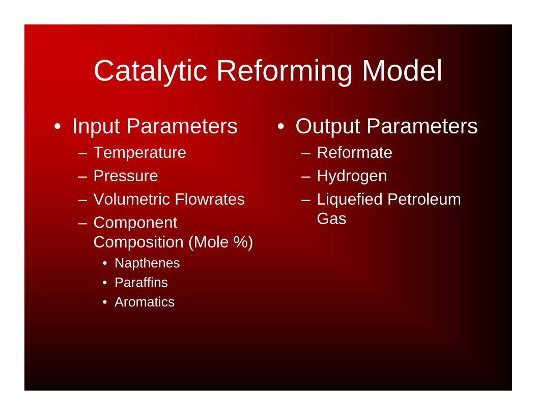
Catalytic Reforming Model
• Input Parameters– Temperature– Pressure– Volumetric Flowrates– Component
Composition (Mole %)• Napthenes• Paraffins• Aromatics
• Output Parameters– Reformate– Hydrogen– Liquefied Petroleum
Gas
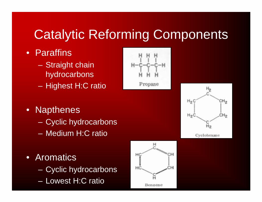
Catalytic Reforming Components• Paraffins
– Straight chain hydrocarbons
– Highest H:C ratio
• Napthenes– Cyclic hydrocarbons – Medium H:C ratio
• Aromatics – Cyclic hydrocarbons– Lowest H:C ratio
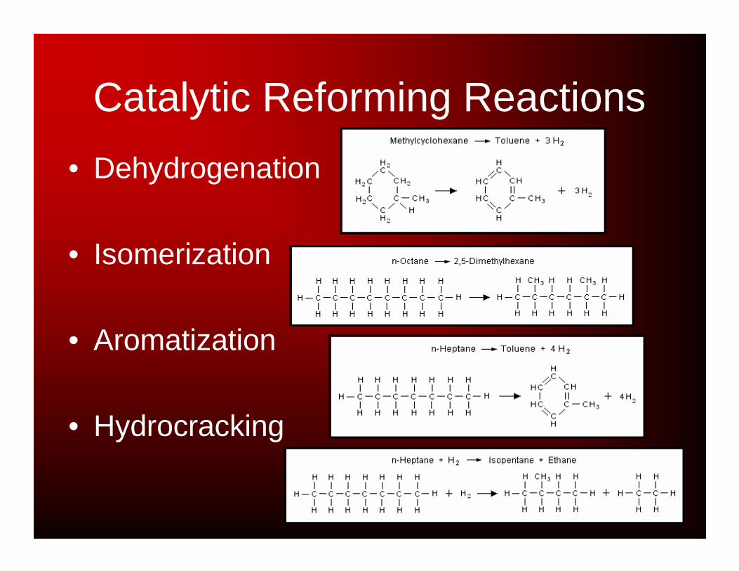
Catalytic Reforming Reactions
• Dehydrogenation
• Isomerization
• Aromatization
• Hydrocracking
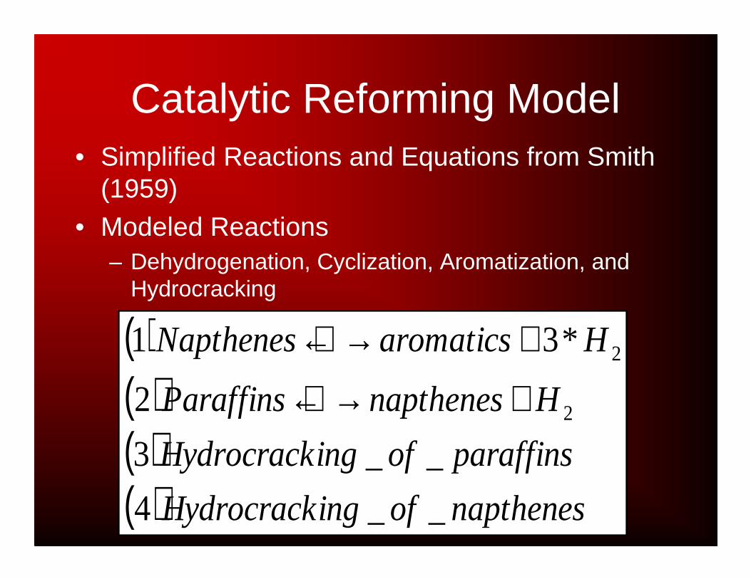
Catalytic Reforming Model• Simplified Reactions and Equations from Smith
(1959)• Modeled Reactions
– Dehydrogenation, Cyclization, Aromatization, and Hydrocracking
( )( )( )( ) napthenesofingHydrocrack
paraffinsofingHydrocrack
HnapthenesParaffins
HaromaticsNapthenes
__4
__3
2
*31
2
2
+→←
+→←
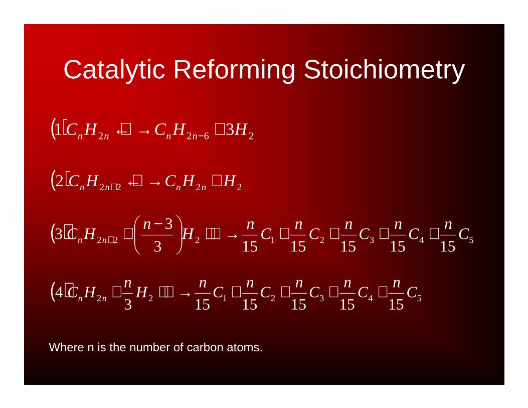
Catalytic Reforming Stoichiometry
( ) 5432122 151515151534 C
nC
nC
nC
nC
nH
nHC nn ++++→+
( ) 54321222 15151515153
33 C
nC
nC
nC
nC
nH
nHC nn ++++→
−++
( ) 22222 HHCHC nnnn +→←+
( ) 2622 31 HHCHC nnnn +→← −
Where n is the number of carbon atoms.

Catalytic Reforming Empirical Kinetic Model
[ ]( )( )( )atmcatlbhr
moles
Tk P ._
,34750
21.23exp1 =
−=)
[ ]( )( )( )22._
,59600
98.35expatmcatlbhr
moles
TkP =
−=)
[ ]( )( )._,
6230097.42exp43 catlbhr
moles
Tkk PP =
−==))
[ ] 33
1 ,46045
15.46exp*
atmTP
PPK
N
HAP =
−==
[ ] 12 ,12.7
8000exp
*−=
−== atmTPP
PK
HN
PP
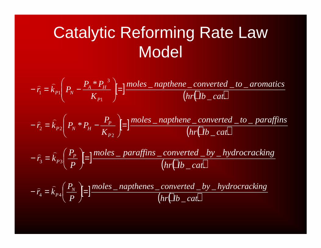
Catalytic Reforming Rate Law Model
[ ] ( )( )._
____*
222 catlbhr
paraffinstoconvertednapthenemoles
K
PPPkr
P
PHNP =
−=−
))
[ ] ( )( )._
____33 catlbhr
inghydrocrackbyconvertedparaffinsmoles
P
Pkr P
P =
=−))
[ ] ( )( )._
____*
1
3
11 catlbhr
aromaticstoconvertednapthenemoles
K
PPPkr
P
HANP =
−=−
))
[ ] ( )( )._
____44 catlbhr
inghydrocrackbyconvertednapthenesmoles
P
Pkr N
P =
=−))

Excel Model
Partial Flowrates
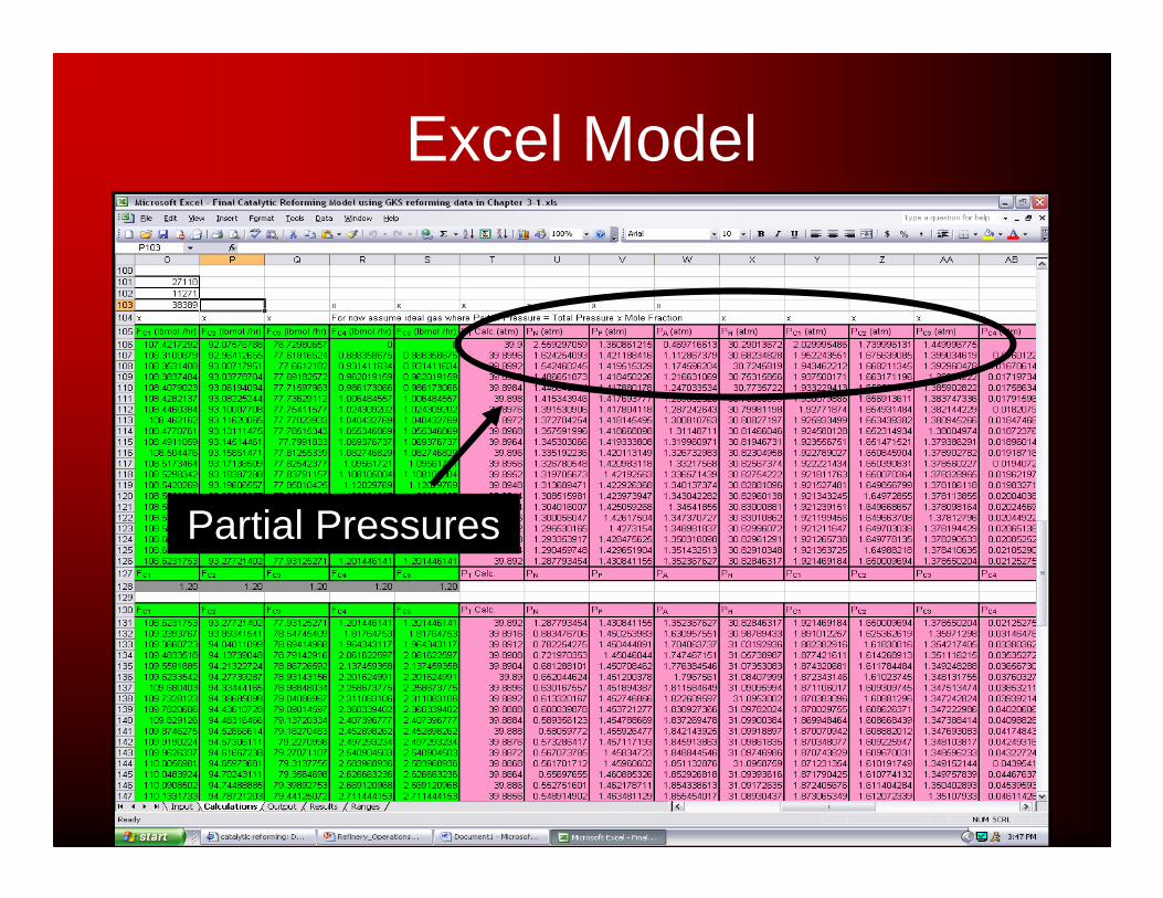
Excel Model
Partial Pressures

Excel Model
Rate of Reaction Rate Constants
Equilibrium Constants
GAMS Model
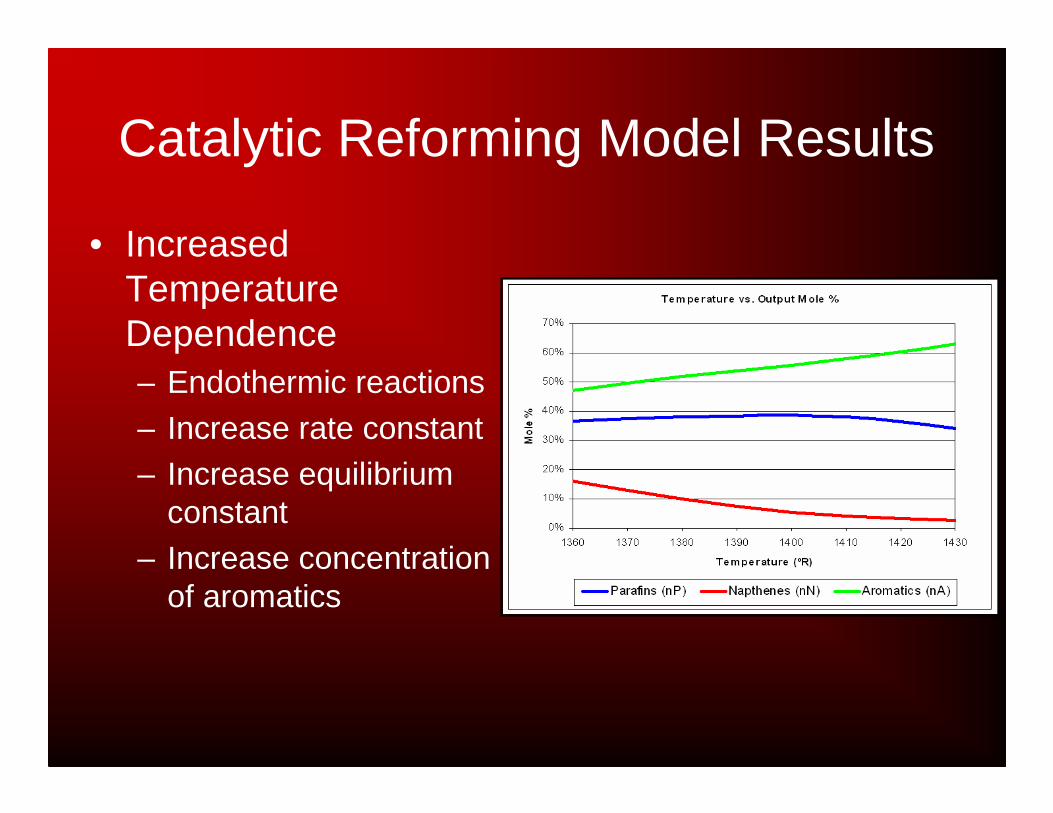
Catalytic Reforming Model Results
• Increased Temperature Dependence– Endothermic reactions– Increase rate constant– Increase equilibrium
constant– Increase concentration
of aromatics

Catalytic Reforming Model Results
• Decreased Pressure Dependence– Increase overall
reaction rate for hydrocracking
– Increases concentration of aromatics

Isomerization• Gas-phase catalyzed reaction
• Transforms a molecule into a different isomer• Transforms straight chained isomers into
branched isomers• Increases octane rating of gasoline

Isomerization Unit
• 2 types of catalysts most commonly used– Platinum/chlorinated
alumina
– Platinum/zeolite

Isomerization Unit
• Feeds– Butanes
– Pentanes– Hexanes
– Small amounts Benzene– Make-up Hydrogen
• Products– Branched alkanes

Isomerization Unit
isomerization stabilization deisohexanizerFeed
H2 make up
Fuel gas
isomerate
recycle
isomerate
H2 recycle

Isomerization
Isomerate
n-C6 Recycle
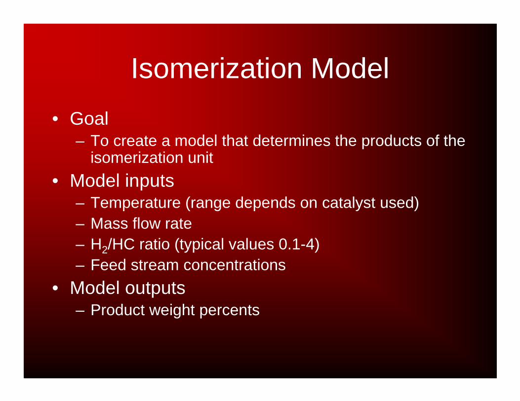
Isomerization Model
• Goal – To create a model that determines the products of the
isomerization unit
• Model inputs– Temperature (range depends on catalyst used)– Mass flow rate– H2/HC ratio (typical values 0.1-4)– Feed stream concentrations
• Model outputs– Product weight percents

Isomerization Model
• Modeling– Determine feed partial pressures
– N-Butane kinetic model– N-Pentane kinetic model
– N-Hexane kinetic model
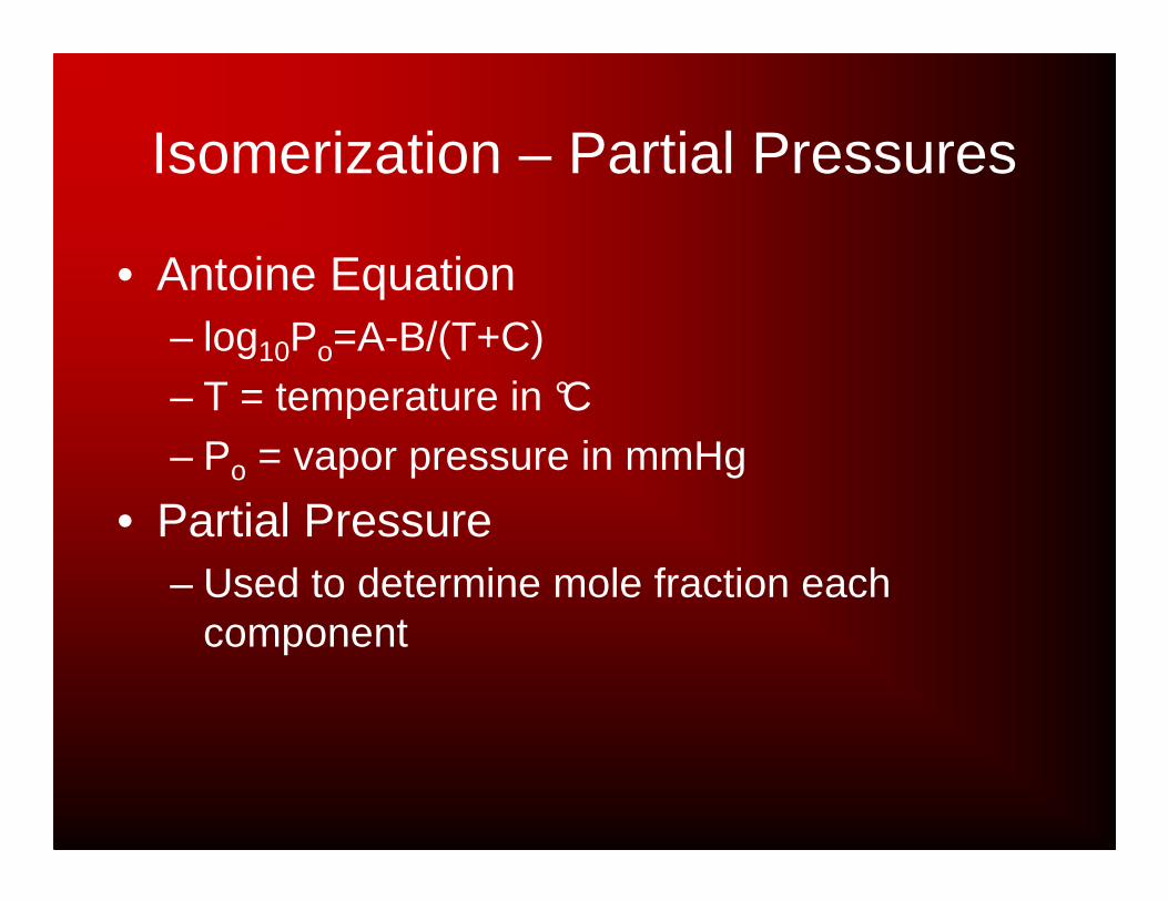
Isomerization – Partial Pressures
• Antoine Equation – log10Po=A-B/(T+C)
– T = temperature in °C– Po = vapor pressure in mmHg
• Partial Pressure– Used to determine mole fraction each
component
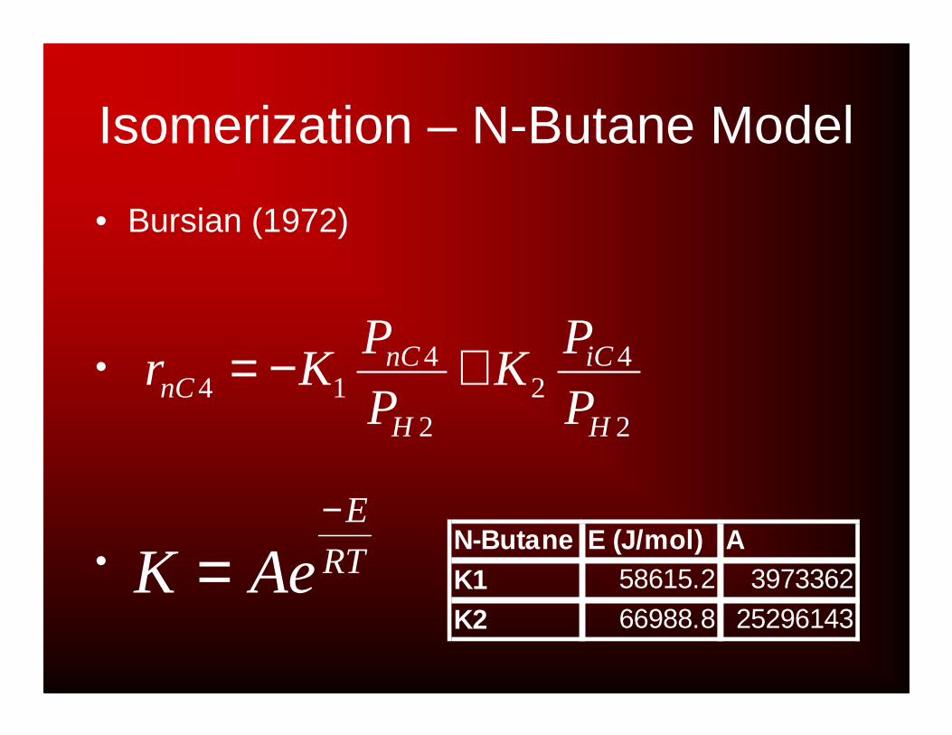
Isomerization – N-Butane Model
• Bursian (1972)
•
•
2
42
2
414
H
iC
H
nCnC P
PK
P
PKr +−=
N-Butane E (J/mol) AK1 58615.2 3973362
K2 66988.8 25296143
RT
E
AeK−
=

Isomerization - N-Pentane Model
• Aleksandrov (1976)
•
• ])1(][0000197.0)([ 55125.0
2
525
299.11861
iCeqnCeqnC
nC
RTReq
CKCKtH
CKr
eK
+−−−=
=−
n-pentane E (kcal/mol) E (J/mol) AK1 10.1 42.2887 4023.872K2 119.5 500.3465 7331.974

Isomerization - N-Hexane Model
• Cheng-Lie (1991)
• ∑∑==
+⋅
−=
5
1,
5
1,
jjjii
jij
i CKCKdt
dC
52,2-DMB
42,3-DMB
32-MP
23-MP
1n-Hexane

Isomerization Model
• Rate equations solved using finite integration
• Output - concentrations of various isomers in product stream
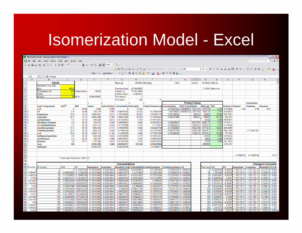
Isomerization Model - Excel
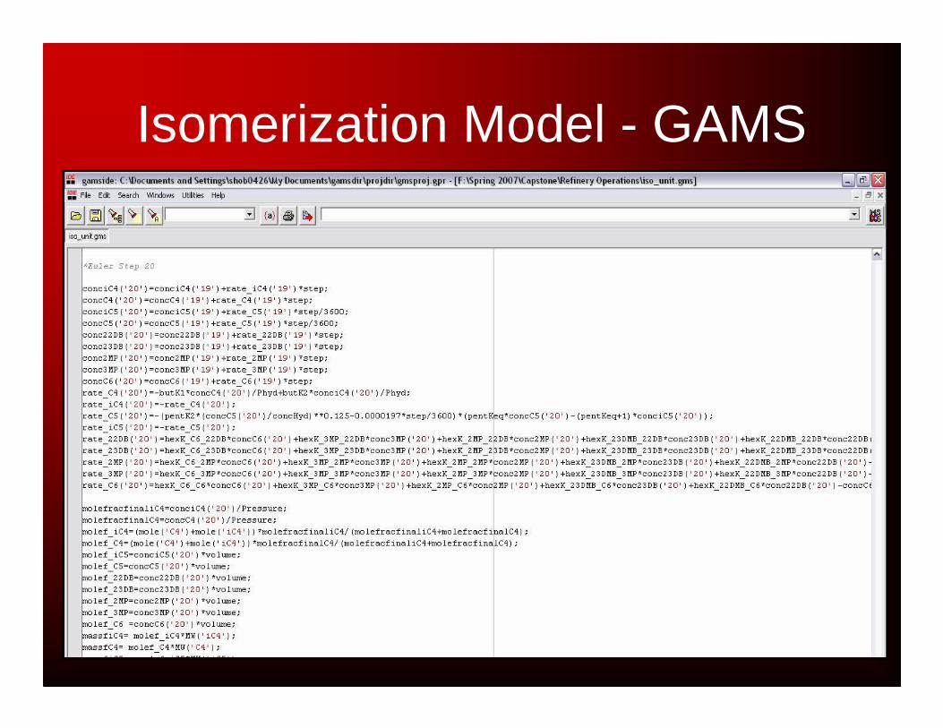
Isomerization Model - GAMS

Isomerization Model Results
• Temperature Increase– Pt/Chlorinated Alumina 120-180°C– Pt/Zeolite 250-270°C
Octane # vs. Temperature
70.000
72.000
74.000
76.000
78.000
80.000
82.000
84.000
110 130 150 170 190 210 230 250 270 290
Temperature (C)
Oct
ane
Nu
mb
er
Octane Rating After Unit

Isomerization Model Results
• H2/HC Ratio increase– Range 0.1-4
Octane # vs. H2/HC
70
72
74
76
78
80
82
84
0 0.5 1 1.5 2 2.5 3 3.5 4
H2/HC
Oct
ane
#
Linear (Octane Number After Unit)
Linear (Octane Number Before Unit)
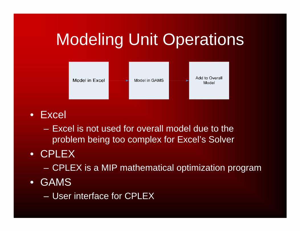
Modeling Unit Operations
• Excel– Excel is not used for overall model due to the
problem being too complex for Excel’s Solver
• CPLEX – CPLEX is a MIP mathematical optimization program
• GAMS– User interface for CPLEX
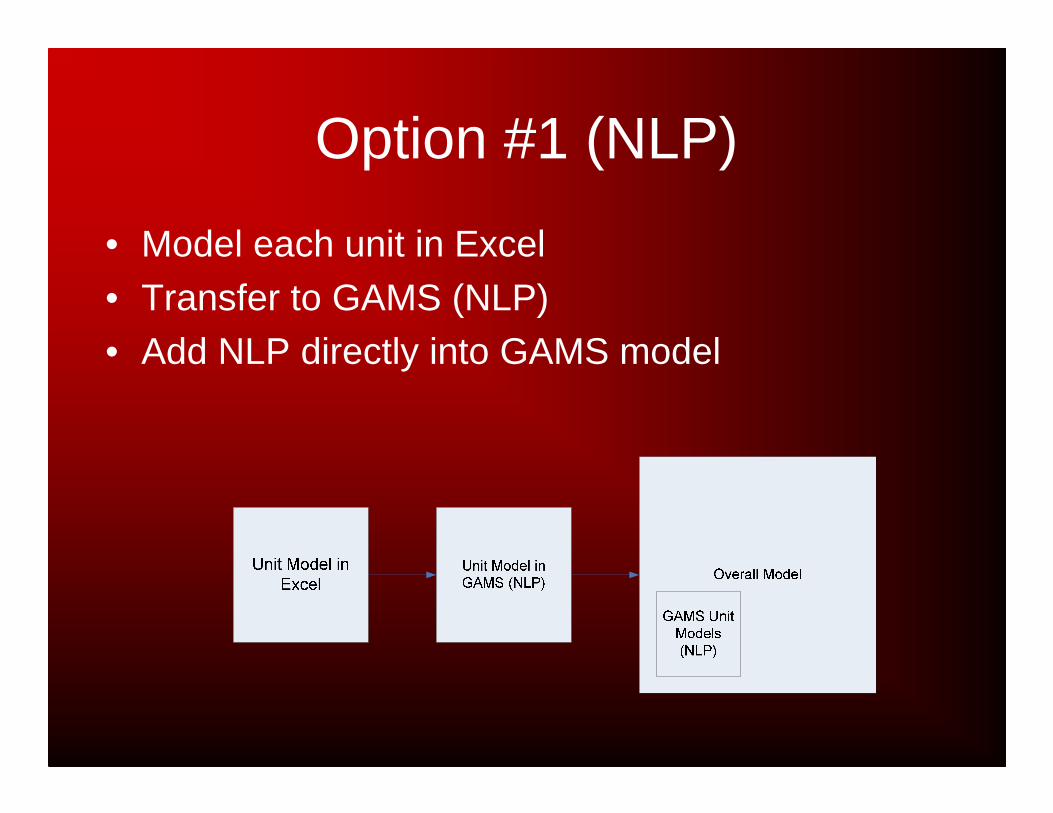
Option #1 (NLP)
• Model each unit in Excel
• Transfer to GAMS (NLP)• Add NLP directly into GAMS model
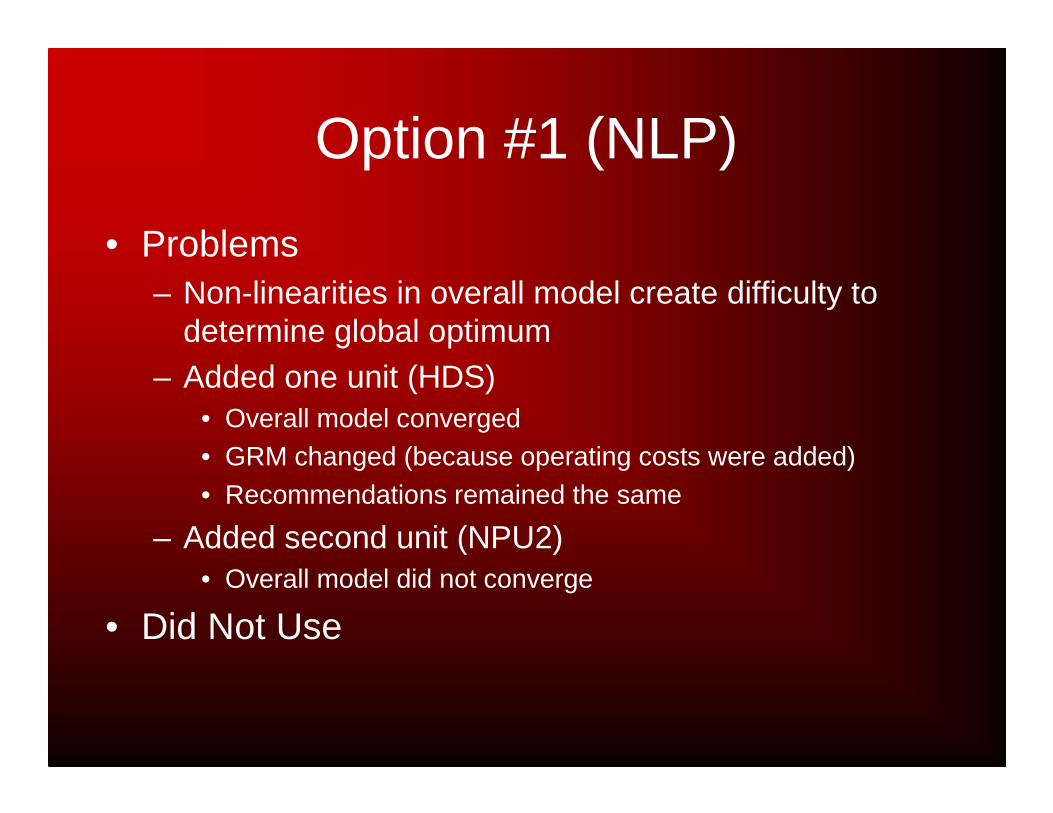
Option #1 (NLP)
• Problems– Non-linearities in overall model create difficulty to
determine global optimum– Added one unit (HDS)
• Overall model converged• GRM changed (because operating costs were added)• Recommendations remained the same
– Added second unit (NPU2)• Overall model did not converge
• Did Not Use
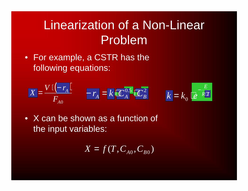
• For example, a CSTR has the following equations:
• X can be shown as a function of the input variables:
TR
E
ekk ⋅−
⋅= 0
( )0A
A
F
rVX
−⋅=
Linearization of a Non-Linear Problem
),,( 00 BA CCTfX =
25.0BAA CCkr ⋅⋅=−
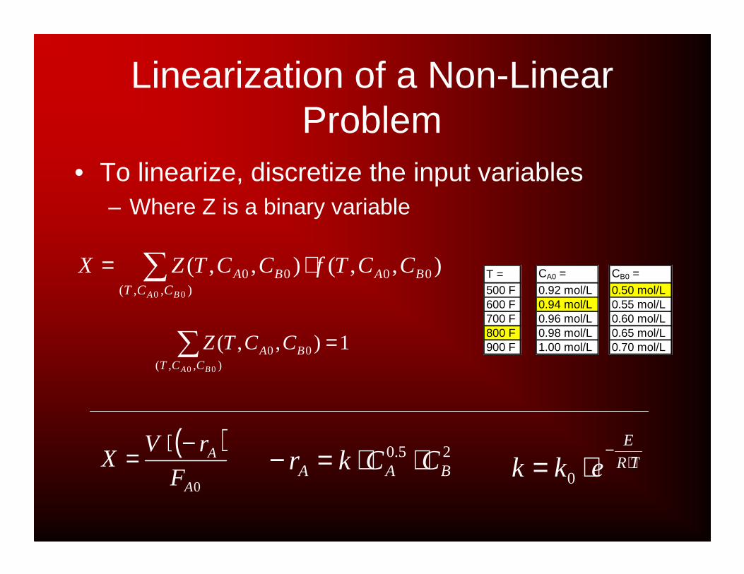
Linearization of a Non-Linear Problem
• To linearize, discretize the input variables– Where Z is a binary variable
∑ ⋅=),,(
0000
00
),,(),,(BA CCT
BABA CCTfCCTZX
TR
E
ekk ⋅−
⋅= 0
25.0BAA CCkr ⋅⋅=−
( )0A
A
F
rVX
−⋅=
1),,(),,(
00
00
=∑BA CCT
BA CCTZ
T =500 F600 F700 F800 F900 F
CA0 =
0.92 mol/L0.94 mol/L0.96 mol/L0.98 mol/L1.00 mol/L
CB0 =
0.50 mol/L0.55 mol/L0.60 mol/L0.65 mol/L0.70 mol/L

Non-Linearities in Unit Operations
• CSTR
• Catalytic Reformer
TR
E
ekk ⋅−
⋅= 0
( )0A
A
F
rVX
−⋅= 25.0BAA CCkr ⋅⋅=−
−=T
kP
3475021.23exp1
)
−=T
kP
5960098.35exp2
)
−==T
kk PP
6230097.42exp43
))
N
HAP P
PPK
3
1
*=HN
PP PP
PK
*2 =
−=−
222 *
P
PHNP K
PPPkr
))
=−P
Pkr P
P33
))
−=−
1
3
11
*
P
HANP K
PPPkr
))
=−P
Pkr N
P44
))

Option #2 (MIP)
• Take Excel model
• Write MIP utilizing table of possible variables• Add MIP directly into GAMS model
Unit Model in Excel Unit Model in GAMS (MIP)
Overall Model
GAMS Unit Models (MIP)
Table of Possible
Operating Conditions
Table of Possible
Operating Conditions
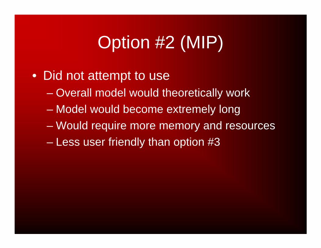
Option #2 (MIP)
• Did not attempt to use– Overall model would theoretically work
– Model would become extremely long– Would require more memory and resources
– Less user friendly than option #3
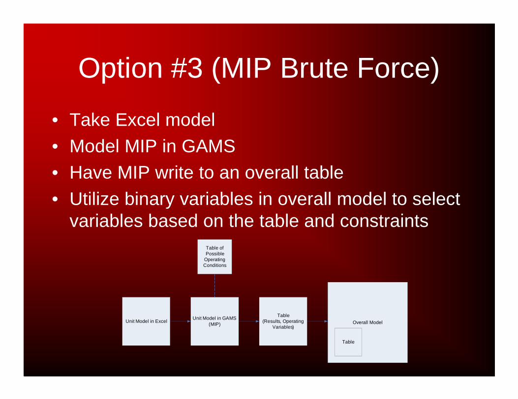
Option #3 (MIP Brute Force)
• Take Excel model
• Model MIP in GAMS• Have MIP write to an overall table
• Utilize binary variables in overall model to select variables based on the table and constraints
Unit Model in ExcelUnit Model in GAMS
(MIP) Overall ModelTable
(Results, Operating Variables)
Table
Table of Possible
Operating Conditions

Table Generation
∑ ⋅=),,(
0000
00
),,(),,(BA CCT
BABA CCTXCCTZX
T = CA0 = 0.50 mol/L 0.55 mol/L 0.60 mol/L 0.65 mol/L 0.70 mol/L500 F 0.92 mol/L 0.74 0.22 0.75 0.54 0.93500 F 0.94 mol/L 0.10 0.39 0.79 0.32 0.38500 F 0.96 mol/L 0.72 0.70 0.06 0.28 0.22500 F 0.98 mol/L 0.54 0.57 0.53 0.24 0.22500 F 1.00 mol/L 0.91 0.41 0.80 0.66 0.97600 F 0.92 mol/L 0.33 0.12 0.09 0.77 0.08600 F 0.94 mol/L 0.04 0.70 0.78 0.79 0.58600 F 0.96 mol/L 0.48 1.00 0.00 0.52 0.24600 F 0.98 mol/L 0.86 0.40 0.85 0.10 0.27600 F 1.00 mol/L 0.15 0.42 0.91 0.72 0.59700 F 0.92 mol/L 0.00 0.62 0.69 0.29 0.85700 F 0.94 mol/L 0.73 0.78 0.47 0.93 0.55700 F 0.96 mol/L 0.83 0.45 0.46 0.54 0.64700 F 0.98 mol/L 0.94 0.43 0.69 0.25 0.88700 F 1.00 mol/L 0.25 0.01 0.61 0.26 0.07800 F 0.92 mol/L 0.25 0.64 0.55 0.40 0.68800 F 0.94 mol/L 0.37 0.87 0.14 0.31 0.96800 F 0.96 mol/L 0.52 0.58 0.37 0.61 0.71800 F 0.98 mol/L 0.46 0.20 0.17 0.99 0.37800 F 1.00 mol/L 0.04 0.82 0.81 0.81 0.86900 F 0.92 mol/L 0.83 0.39 0.50 0.57 0.10900 F 0.94 mol/L 0.27 0.52 0.35 0.81 0.96900 F 0.96 mol/L 0.71 0.09 0.63 0.45 0.03900 F 0.98 mol/L 0.61 0.47 0.30 0.29 0.09900 F 1.00 mol/L 0.30 0.35 0.52 0.84 0.02
CB0 =

Option #3 (MIP Brute Force)
• Currently being used– Offers ease of use for the overall model
– Drawback - more files are required to run the model
• 26 tables utilized
Specific Modeling Issues
• “Best Choice” scenario• Mass Balance• Blending• Additions

“Best Choice” Scenario
• Unit operations flow rates chosen by which scenario is nearest to the actual flow rate
• Allows for degrees of freedom in crude purchasing
Foverall
Ffg,out
Fref,unit
Flpg,unit
Ffg,unit
Flpg,out
Fref,out
Funit

“Best Choice” Scenario
• F = flow rates• d = difference between discretized unit flow rates
dFF overallunit ≤−dFF unitoverall ≤−
F =15000 m3/d16000 m3/d17000 m3/d18000 m3/d19000 m3/d
5002
1500016000..
2
12 =−=−= geFF
d

Mass Balance (CRU2, CRU3, ISOU)
Foverall
Ffg,out
• Solving the mass balance (2 options)
– Foverall = Fout
• Requires a non-linear equation (Z*Foverall)• Linearization possible, but requires massive
amounts of memory (takes the program a long time to run)
Fref,unit
Flpg,unit
Ffg,unit
Flpg,out
Fref,out
Funit
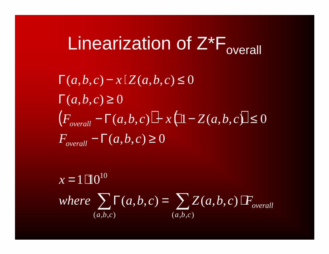
Linearization of Z*Foverall
( ) ( )
∑∑ ⋅=Γ⋅=
≥Γ−≤−⋅−Γ−
≥Γ≤⋅−Γ
),,(),,(
10
),,(),,(
101
0),,(
0),,(1),,(
0),,(
0),,(),,(
cbaoverall
cba
overall
overall
FcbaZcbawhere
x
cbaF
cbaZxcbaF
cba
cbaZxcba
Mass Balance (CRU2, CRU3, ISOU)
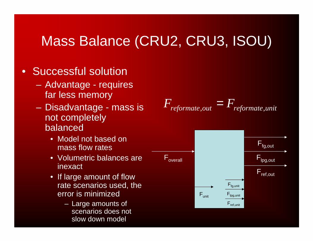
• Successful solution– Advantage - requires
far less memory– Disadvantage - mass is
not completely balanced
• Model not based on mass flow rates
• Volumetric balances are inexact
• If large amount of flow rate scenarios used, the error is minimized
– Large amounts of scenarios does not slow down model
unitreformateoutreformate FF ,, =
Foverall
Funit
Ffg,out
Fref,unit
Flpg,unit
Ffg,unit
Flpg,out
Fref,out
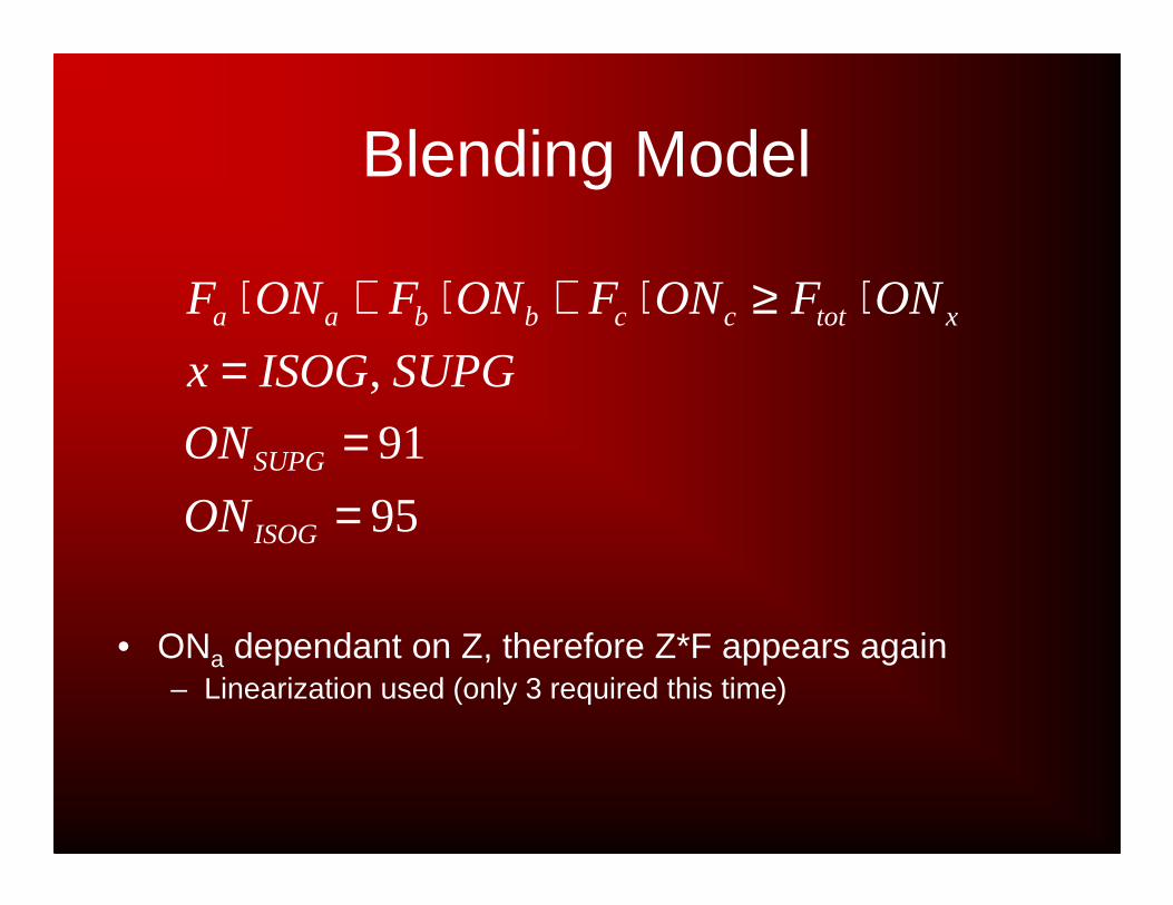
Blending Model
95
91
,
==
=⋅≥⋅+⋅+⋅
ISOG
SUPG
xtotccbbaa
ON
ON
SUPGISOGx
ONFONFONFONF
• ONa dependant on Z, therefore Z*F appears again– Linearization used (only 3 required this time)

Linearization of Z*Foverall
( ) ( )
∑∑ ⋅=Γ⋅=
≥Γ−≤−⋅−Γ−
≥Γ≤⋅−Γ
),,(),,(
10
),,(),,(
101
0),,(
0),,(1),,(
0),,(
0),,(),,(
cbaoverall
cba
overall
overall
FcbaZcbawhere
x
cbaF
cbaZxcbaF
cba
cbaZxcba

Additions
• Revised Fuel Balance– Fuel Gas and Fuel Oil burned
• Added Operating Costs associated with compression
• Added Hydrogen Balance
Results
• Executed using CPLEX
– Approximately 50 minutes to reach integer solution
– Approximately 2 hours to reach optimal solution

It Works!
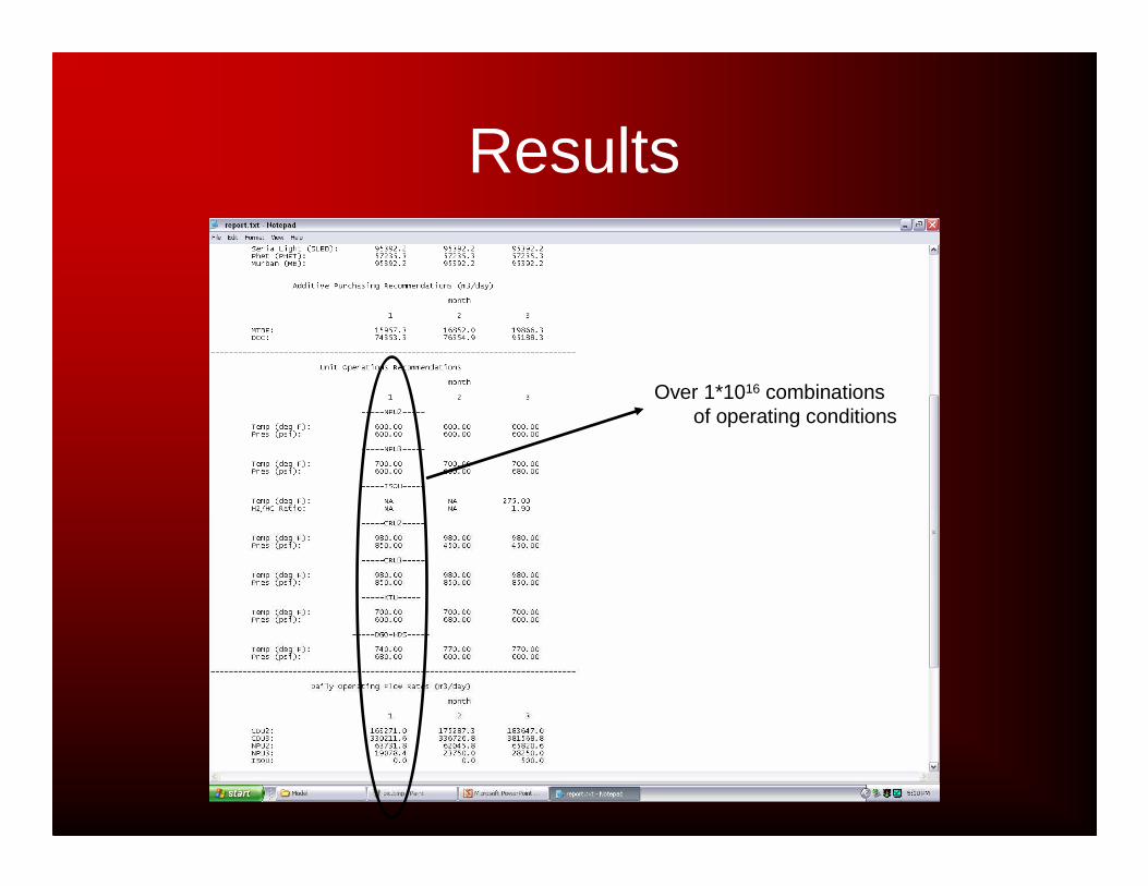
Results
Over 1*1016 combinations of operating conditions
Planning
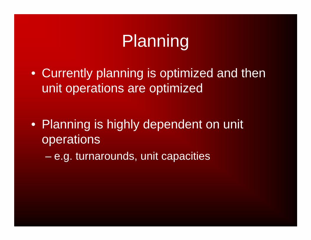
• Currently planning is optimized and then unit operations are optimized
• Planning is highly dependent on unit operations– e.g. turnarounds, unit capacities
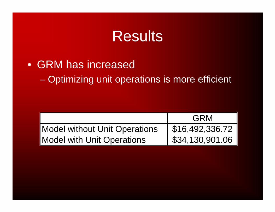
Results
• GRM has increased – Optimizing unit operations is more efficient
GRMModel without Unit Operations $16,492,336.72Model with Unit Operations $34,130,901.06

Results
• Purchased crudes and intermediates
1 2 3Oman (OM): 167734.3 167339.3 165082.6Tapis (TP): 13427.7 14317 19397.5Labuan (LB): 0 0 0Seria Light (SLEB): 95392.2 95392.2 95392.2Phet (PHET): 57235.3 57235.3 57235.3Murban (MB): 95392.2 95392.2 95392.2MTBE: 13662 13700.7 13921.7DCC: 68088 68301.8 69523.2
Model without Unit Operations1 2 3
Oman (OM): 244486.2 262303.1 267899.8Tapis (TP): 32853.3 41126.2 47392.2Labuan (LB): 0 0 9041.4Seria Light (SLEB): 95392.2 95392.2 95392.2Phet (PHET): 57235.3 57235.3 57235.3Murban (MB): 95392.2 95392.2 95392.2MTBE: 18266 19392.8 20404.2DCC: 87059.5 91153.7 93941.2
Model with Unit Operations
Results
HDS
FOVS
FO2
GASOLINEPOOL
DIESELPOOL
CDU2
CDU3
MB
FG
LPG Naphtha FO
Kero DO
NPU
LN
HN
ISOU
CRU
HN
FG
REF
LPG
KTU
ISO
LN
Kero
IHSD
MTBET
DCCT
ISOG
SUPG
HSD
JP1
FO1
Products
Intermediates
PHET
SLEB
LB
TP
OM
Crudes
Kero
FO
Kero

Discussion
Reformer Sensitivity
86
88
90
92
94
96
98
100
Oct
ane
Nu
mb
er
Varying Flow (15-25 Mm3/day)Varying Pressure (400-800 psi)Varying Temperature (800-980 °F)Linear (Varying Flow (15-25 Mm3/day))Poly. (Varying Pressure (400-800 psi))Poly. (Varying Temperature (800-980 °F))
Discussion
• Optimizing unit operations adds another dimension to optimize refinery processing
• Can provide more thorough insight for decision making

Acknowledgments
• Dr. Miguel Bagajewicz• DuyQuang Nguyen• Mike Mills
• Sunoco Refinery (Tulsa, OK)– John Paris

Please, No Questions!
….Just Kidding