Reference Design and Comparative Analysis of Model ...

© Faculty of Mechanical Engineering, Belgrade. All rights reserved FME Transactions (2020) 48, 329-341 329

Received: October 2019, Accepted: February 2020 Correspondence to: Prof. C. Bharatiraja, Department of Electrical and Electronics Engineering, SRM Institute of Science and Technology,Tamil Nadu, India E-mail: [email protected] doi:10.5937/fme2002329F

Abu Feyo Lecturer

Faculty of Electrical and Computer Engineering, Jimma Institute of Technology,Jimma University,

Ethiopia

Amruth Ramesh Thelkar Assistant Professor

Faculty of Electrical and Computer Engineering, Jimma Institute of Technology,Jimma University,

Ethiopia

C Bharatiraja Associate Professor

Department of Electrical and Electronics SRM Institute of Science and Technology,

India Visiting Researcher, Engineering

Department of Electrical, University of South Africa, South Africa

Yusuff Adedayo

Associate Professor Department of Electrical, Florida Campus

Unisa South Africa, South Africa

Reference Design and Comparative Analysis of Model Reference Adaptive Control for Steam Turbine Speed Control This paper presents the mathematical modeling of the steam turbine unit with the fuzzy controller in an isolated operating condition, especially in nuclear power plants. The water level in the steam generator is one of the main causes for the shutdown of the reactor. This problem has been of immense concern during the past years as the steam generator and governor speed control is a highly nonlinear system showing inverse response dynamics. In the present research a simulink model of turbine with fuzzy controller is designed. The results are compared and analyzed with MRAC design technique to determine better methodological solution for the steam turbine speed control and achieved, time to the adaption effectiveness of 0.3 to 2.5% with and without GDB. Improved set point tracking and control with respect to turbine speed are demonstrated for the cases when governor dead-band is present and absent. Keywords Steam turbine, Governor Dead Band (GDB), Model Reference Adaptive Control (MRAC), Lyapunov rule, Fuzzy Logic Control (FLC)..

1. INTRODUCTION

The steam turbines may the used for the applications to drive an electric generator or equipment such as boiler feedwater pumps, process pumps, air compressors, paper mills and refrigeration chillers. The Rankine cycle and thermodynamic principles are the fundamental basis for steam turbines, in conventional power generating stations where water is first pumped to elevated pressure, which is medium to high pressure, depending on the type of turbine unit and then most frequently superheated. For the commercial and industrial applications, the pressu-rized steam is expanded to lower pressure in a multistage turbine, then exhausted either to a condenser at vacuum conditions or into an intermediate temperature steam distribution system and condensate to utilized back. The measured stimulus and response samples of turbine or plants, used for system identification, involve building a mathematical model of dynamic system. System identification is a process of acquiring, formatting, processing and identifying mathematical models based on raw data from the real-world system. System identification of an interacting series process for real-time model predictive control is done and many critical challenging problems are occurring due to the non-linear behaviour in most of the nuclear power plant and chemical industries. Therefore, traditional control techniques are needed for most of the chemical process industries. Conical tanks exhibit non-linear behaviour which is suitable for food process industries, concrete mixing industries, hydrometallurgical industries and

waste water treatment industries. [1,2]. The industrial processes are complex in nature. It is

difficult to develop a closed loop control model. Also, the human operator is often required to provide online adjustment, which makes the process performance greatly dependent upon the experience of the individual operator. It would be extremely useful if some kind of systematic methodology can be developed for the process control model that is suited to this kind of industrial process. There are some variables in conti-nuous DCS (distributed control system) that suffer from several unexpected disturbances during the operation (noise, parameter variation, model uncertainties), so the human supervision (adjustment) is necessary. If the operator has a little experience, the system may be damaged or operated at lower efficiency. One such system is the control of steam turbine speed using PI controller as the main controller for controlling the process variable. The process is exposed to unexpected conditions and the controller fails to maintain the process variable in a satisfied manner and retuning of the controller becomes necessary. In a nuclear power plant, the water level in the steam generator is one of the main causes that shutdown the reactor, this problem has been of great concern for many years as the steam gene-rator and governor speed control is a highly nonlinear system showing inverse response dynamics. The speed governor dead band has significant effect on the dynamic performance of load frequency system[3,4].

To cope with the above listed problems, much research has been devoted with various control tech-niques. Conventional controllers are widely used in industries due to low cost, ease of implementation and tuning. The performance of these conventional contro-llers has been enhanced by tuning various methods viz Zeigler - Nichol’s and simplex method. Even though, but the conventional PID controllers with fixed gain are

330 ▪ VOL. 48, No 2, 2020 FME Transactions

unable to cope up with the problems discussed above. The use of conventional controllers with artificial intel-ligence, for control of parameters to get optimal plant performance has been enumerated in this paper[5,6,7,8].

Adaptation of PID controller using techniques like fuzzy logic, the DSP-based laboratory model of Hybrid Fuzzy-PID controller using genetic optimization for high-performance motor drives [9,10] and Neuro fuzzy controller (ANFIS) for speed control of isolated steam turbine had been proposed in the earlier research [11,12] and later on, the neural network is applied to develop the PID controllers to enhance the dynamic charac-teristics of controller [13]. Research gaps highlights the complete adaptive nature, specific adaptive control tech-niques, now a days, the adaptive control schemes are making their place where the conventional control sys-tem fails with the uncertainty situations, like reference design and analysis of model reference adaptive control (MRAC) for steam turbine speed control loads, inertias and the forces acting on system, changes drastically, possibility of unpredictable and sudden faults, possibi-lity of frequent or unanticipated disturbances.

Among many adaptive control schemes, this paper mainly deals with the combination of model reference adaptive control (MRAC) approach with Lyapunov rule as adjusting mechanism and fuzzy. In MRAC, the output response is forced to track the response of a refe-rence model, irrespective of plant parameter variations, eventhough, the disadvantage of MRAC scheme is time to adapt and leads to oscillations after a certain period, however, fuzzy control methods have a advantage of robustness, which have been demonstrated through the industrial applications [14,15].

Another method, popular in recent years, is based on fuzzy neural network. It is proved that both methods ensure good characteristics, yet the fuzzy neural net-work requires less control effort. Fuzzy neural networks combine the capability of fuzzy reasoning and the abi-lity of neural networks learning from processes [16,17]. On the other hand, the combination of the fuzzy control base design and the MRAC control causes the reduction of the fuzzy rules significantly. The adaptive fuzzy con-troller is able to ensure very good dynamical perfor-mance of different industrial objects including electrical drives[18,19].

The combination of adaptive and fuzzy control is to work in situations where there is a large uncertainty or unknown variation in plant parameters and structures. A stable speed is useful for the operation of generator under loaded and no load condition. This reserach identifies the parameters of the steam turbine speed control, compare with the fuzzy logic techniques, MRAC model and to choose the appropriate control method among the two listed techniques with and without GDB(Governor Dead Band).

The paper is divided into five sections. In section 2, steam turbine mathematical model is described. Section 3, model reference adaptive control simmulink design is presented. Section 4 design of fuzzy logic controller, section 5 results and discussion of the overall paper is presented. In the next section, the concluding remarks are given to summarize the contribution of the work.

2. MATHEMATICAL MODEL OF THE STEAM TURBINE

Tandem-compound single-reheat steam turbine assembly is composed of four stages in line on the same shaft with several casings. The superheated steam enters the high-pressure stage (HP) where it expands through the small diameter rotor blades before exiting and being returned to the boiler. In the boiler the steam is superheated and is directed to the intermediate pressure stage (IP). Here, it expands through larger diameter rotor blades exiting to the low-pressure turbines. In the final stage there are two identical sets of low-pressure turbines (Dual LP), the exiting steam from the IP turbine is divided equally between the two turbines passing through quite large diameter rotors and blades along with that main inlet stop valves (MSV), main inlet control (governor) valves (CV), reheater stop valves (RSV), reheater intercept valves (IV) shown in figure 1[3]. The steam turbine mathematical model has two parts: first, simplified transfer function of a linear steam turbine which associates with the change in mechanical power ∆PM, the changes in steam valve position ∆PGV and second, of turbine-governor model, considering nonlinear characteristics.

G

MSV

CV

HP IP LP LP

Condenser

Cross Over

RH

Figue 1. Tandem compound single reheat steam turbine 2.1 Transfer Function of a Linear Single reheat

Steam Turbine The model for a single reheat tandem-compound steam turbine shown in figure 2 is presented in this paper. Large steam turbines are used in fossil fuel power plants, fossil fuel plants typically burns coal to heat a boiler that produces high boiler that produces high-temperature, high-pressure steam, which is passed through the turbine.

FHP FMP FLP

GHP GMP GLP

+ +

∆PGV

PHP PMP PLP

PM

Figue 2. Single Reheat tandem-compound steam turbine model

The actual transfer function for steam turbine can be considered as

HPHP

sTG

+=

1

1

(1)

MP

MPsT

G+

=1

1 (2)

FME Transactions VOL. 48, No 2, 2020 ▪ 331

11

LPLPsT

G =+

(3)

where GHP, GMP/ and GLP are actual transfer function of high pressure, medium pressure and low-pressure tur-bines respectively and THP/TCH-Steam chest time cons-tant, TRH-Reheat time constant and TLP or TCO -Crossover piping time constant as described in table 1.

FHP +FMP+FLP=1 (4)

Expression (4) indicates the fraction of power gene-rated in the HP section, medium section and the low section, and its summation should be equal to 1. Sub-stituting the values for the parameters from the table 1.

15.0

3.0)(

+=

ssGHP (5)

125.0

4.0)(

+=

ssGIP (6)

11.0

3.0)(

+=

ssGLP (7)

The overall transfer function for the system, desc-ribes the mechanical power with the change in steam valve position, where FIP=1-FHP. Assume TCO is negli-gible in comparison with TRH and TCH, then the CV characteristics is linear. Table 1. Steam turbine parameter list [12]

Parameter Unit Description Default Min Max

FHP p.u

High pressure turbine power fraction

0.3 -2 1

FMP p.u

Medium pressure turbine power fraction

0.4 0 3

FLP p.u

Low pressure turbine power fraction

0.3 0 1

TRH Sec Reheat time constant 0.5 0.01 20

THP Sec Steam Chest time constant 0.25 0 1

TLP Sec Crossover piping time constant

0.1 0.01 1

TSM Sec Valve positioner time constant

0.5 0.04 1

1)(2))((3

1)(21)(

)(

+++++++

++++

+=Δ

Δ

+

STTTTTTTTSTTT

FLP

sTTSTT

F

ST

F

sP

sP

CORHCHCORHCHRHCHCORHCH

RHCHRHCH

IP

CH

HP

GV

M

S

1)(21

1)(

)(

+++

−+

+=

Δ

Δ

sTTsTT

F

sT

F

sP

sP

RHCHRHCH

HP

CH

HP

GV

M

Where PM is change in mechanical power, ΔPGV is change in valve position.

)1)(1(

1

)(

)(

CHRH

RHHP

sGV

sM

sTsT

TsF

P

P

++

+

Δ

Δ= (8)

The actual transfer function for steam turbine is obtained after the substitution of values from table 1 and expressions 1, 2 and 3.

( ) 1 (0.3)(0.5) 1.2 82( ) (1 0.5 )(1 0.25 ) 6 8

M

GV

P s s s

P s s s ss

Δ + += =

Δ + + + + (9)

2.2 Typical design model of steam turbine control A typical governor model for steam turbines has two main sections, the governor and steam control valve, whose output is effective control valve area in response to speed deviation of the machine and a section model-ling the turbine, whose input is steam flow and output is mechanical power applied to the rotor. In the block diagram (figure 3), where Gg(s) is a governor transfer function, Gsr(s) is a speed relay transfer function, Gsm(s) is a servo motor transfer function. Gp(s) is a system/plant transfer function.

1

0.5S + 1

1

0.01S + 1

1

0.3S + 1

1.2S + 8

S2 + 6S + 8

ωref ∆Psr ∆PGV PM

Gg(s) Gsr(s) Gsm(s) Gp(s) Figure 3. Typical design model of steam turbine control

Change in valve position to change in speed relay is expressed as,

1

1

)(

)(

+=

Δ

Δ

TsmssPsr

sPGV (10)

where TSM is servo motor time constant. Transfer func-tion of change in speed relay to reference speed, which is product of governor and speed relay transfer function is expressed as,

)(

)(

sref

sPsr

ω

Δ=

1

1

1

1

++ TsrsTgs (11)

Here, Tg and Tsrs are governor and speed relay time constants respectively. Transfer function of mechanical power to steam valve position is considered as

( ) (1 )

( ) (1 )(1 )

M HP RH

GV RH CH

P s sF T

P s T s T s

+=

Δ + + (12)

The overall linear transfer function of a system is obtained as below

( ) (1 ) 1 1 1

( ) (1 )(1 ) 1 1 1

M HP RH

RH CH

P s sF T

ref s T s T S Tgs Tsms Tsrsω

+=

+ + + + +

Substituting the time and power fraction constant from table 1 and expression 12 is obtained as

( ) 1 1.55 4 3 2( ) 112 1180 4752 8320 5333.3

MP s S

ref s SS S S Sω

+=

+ + + + + (13)


2.3 Design model of turbine governor considering the nonlinear characteristics

In fact, due to the factors like machinery manufacturing, the governor has some nonlinear characteristics such as the rate-limit characteristic, amplitude-limit characteris-tic, dead band characteristic, clearance nonlinearity cha-racteristic, etc.. Therefore, describing function approach is used to incorporate the GDB non-linearity which may be expressed by,

( ),Y F x x= (14)

To solve this non-linear problem by DF (Describing Function) approach, it is necessary to make the basic assumption that the variable x, appearing in the non-li-near function ( ),F x x is sufficiently close to a sinuso-idal oscillation and is given as

( )0sin ,x A tω≈ (15)

As the variable function is complex and periodic fu-nction of time, it can be developed in a fourier series as

21, O

o

NF x x N x xF ω

• •⎛ ⎞= + +⎜ ⎟

⎝ ⎠+…. (16)

After neglecting the higher order terms (assuming low pass filter) and backlash nonlinearity is symmetrical about the origin, F0 is zero so the expression (18) will be as follows

10

2( , ) NF x x N x xω

= + (17)

The Fourier co-efficient are derived as N1 = 0.8 and N2 = -0.2 [8]

0

0.2( , ) 0.8F x x x xω

= − (18)

The governor transfer function with linearized dead-band is derived as Equation (19), when the governor transfer function is

( )

( )

1

1

21

01

G sg Tgs

NN s

G sg Tgsω

=+

+

+=

(19)

Substituting the values of N1 and N2 in expression (19) and rearranged Gg(s) as

15.0

064.08.0)(

+

−=

s

ssGg (20)

2.4 Stability analysis of a system using Kharitonov

Stability Checker Kharitonov polynomials are associated with the interval polynomials p(s,a), are expressed as four fixed khari-tonov polynomials.

P+-(s)= a1+ +a2

-s+a3-s2+ a4

+s3+a5+s4+…….

P++(s)= a1+ +a2

+s+a3-s2+ a4

-s3+a5+s4+…….

P-+(s)= a1- +a2

+s+a3+s2+ a4

-s3+a5-s4+…….

P--(s)= a1- +a2

-s+a3+s2+ a4

+s3+a5-s4+…….

Stability analysis steps are narrated as 1. Formu-

lating the interval system model (figure 4) 2. Obtaining the four Kharitonov Polynomials 3. Applying Routh-Hurwitz Criterion to the four polynomials 4. If all the four polynomials are stable, without any sign change in the first column of the R-H Table, then the given interval system is stable[13].

Gg(s) Gsr(s) Gsm(s) Gp(s)++

1/R

∆Psr ∆PGV PMUCPref

Speed droop

Figure 4. Interval system model block diagram

where Gg(s), Gsr(s), Gsm(s) and Gp(s) are transfer of functions of turbine governor, speed relay, servo motor and plant respectively. 2.5 Design of governor transfer function with DB The speed governor produces a position which is assu-med to be a linear, instantaneous indication of speed and is represented by a gain K which is reciprocal of regu-lation or drop. It represents a composite load and speed reference and is assumed constant over the interval of a stability study.

Governor with dead-band is considered as,

15.0

064.08.0

ref(s)

Uc(s)

+

−=

Δ

Δ

s

s

P (21)

With unity feedback the expression 21 becomes,

Uc(s) 0.8 0.064ref(s) 0.436 1.8

sP sΔ −=Δ +

(22)

The speed relay is represented as an integrator with time constant TSR and direct feedback as

Psr(s) 1Uc(s) 0.01 1s

Δ =Δ +

(23)

2.6 Design of servomotor transfer function The servomotor is represented by an integrator with time constant TSM and direct feedback, the valves moves and is physically large, particularly on large units. Rate limiting of the servomotor may occur for large and rapid speed deviation, rate limits are shown at the input to the integrator. Position limits are also indicated and may correspond to wide-open valves or the setting of a load limiter [17]. From expression (10) of change in valve position to change in speed transfer function is obtained as in expression (24).

1

1

)(

)(

+=

Δ

Δ

sTsmsP

sP

sr

GV ; 13.0

1

)(

)(

+=

Δ

Δ

ssPsr

sPGV (24)


The vector-matrix form of the speed governing system is expressed as follows from figure 5.

1 10.5 0.5

100.01

0 0 Pr1 25

0.01 0.01

PGV PGVdPsr Psrdt

efrω

⎡ ⎤−⎢ ⎥Δ Δ⎡ ⎤ ⎡ ⎤= +⎢ ⎥⎢ ⎥ ⎢ ⎥Δ Δ⎢ ⎥⎣ ⎦ ⎣ ⎦−⎢ ⎥⎣ ⎦

⎡ ⎤ Δ⎡ ⎤⎢ ⎥+ ⎢ ⎥⎢ ⎥ Δ− ⎣ ⎦⎢ ⎥⎣ ⎦

(25)

where KG is speed droop gain (state feedback gain) and substituting the numerical values for Tsm, Tsr and KG, the alternative speed governing vector matrix is expre-ssed (27).

1 10.5 0.5

100.01

0 0 Pr1 25

0.01 0.01

PGV PGVdPsr Psrdt

efrω

⎡ ⎤−⎢ ⎥Δ Δ⎡ ⎤ ⎡ ⎤= +⎢ ⎥⎢ ⎥ ⎢ ⎥Δ Δ⎢ ⎥⎣ ⎦ ⎣ ⎦−⎢ ⎥⎣ ⎦

⎡ ⎤ Δ⎡ ⎤⎢ ⎥+ ⎢ ⎥⎢ ⎥ Δ− ⎣ ⎦⎢ ⎥⎣ ⎦

(26)

+∆ωref 1

1+ sTSR

1TSM

+∆Psr 1

s

K ∆ωr

Cvclose

Cvopen Cvmax

Cvmin

∆PGV

Figure 5. Mathematical representation of the speed-governing system 2.7 Design of steam turbine transfer function Each of the turbine section is described by a transfer function GHP(s), GRH(s), GLP(s), and THP, TRH, TLP, it has three sections (High, Medium and Low-pressure sec-tions). Steam Turbine transfer function is considered as

( )

21 1

3 2 1

11HP IP

CH CH RH CH RH

CH RH CO CH RH CH RH CO CH RH CO

tts

ΔPM(s) F F

ΔPGV(s) T s T T (T T )ss

FLP

T T T (T T (T T )T ) (T T T )ss s

G sT

= ++ + + +

++ + + + + + +

=+

where FIP=1-FHP and neglecting the smallest time cons-tants, a simplified transfer function of the steam turbine configuration (with re-heater) is written as follows.

1

(1 )(1 )

( ) 12( ) 1 ( ) 1

M HP HP

GV CH CH RH CH RH

HP RH

RH CH

sF T

sT sT

P s F FP s T s T T T T ss

+

+ +

Δ −= +Δ + + + +

=

The time constants are assumed from table1and expression 27 is obtained as,

86282.1

++

+=

ss

s (27)

Since it is closed loop, the overall transfer function is obtained as

G(s)=)()()()(1

)()()()(

sGsrsGsmsGtsKGg

sGsrsGsmsGtsGg

+ (28)

Substituting the all transfer functions in expression 28 and expression 29 is obtained,

( )

1 1 1 1

1 (1 )(1 ) 1 11 1 1 1

11 (1 )(1 ) 1 1

HP RH

CH RH

HP RH

CH RH

F T

Tgs T s T s Tsms TsrsG s

F TK

Tgs T s T s Tsms Tsrs

+

+ + + + +=

++

+ + + + +

After rearranging and Substituting the values, where K=1, where K=1/R.

( )

( )

(1 )2( 1)( 1)(( ( ) 1))( 1) (1 )

2( 59 ) 344 49235 4 3 2115 1430 6804 14793 16000

HP RH

CH RH CH RH HP RH

G s

F T s

Tsrs Tgs T T T T s Tsms K F T ss

ssG sss s s s

=

+

+ + + + + + + +

− + +=

+ + + + +

(29)

From expression 29, the characteristics equation of the overall transfer function is expressed as below,

5 4 3 2115 1430 6804 14793 16000 0ss s s s+ + + + + = (30)

Using the stability analysis for the above expression, the interval system model is formulated as,

[ ] [ ] [ ][ ] [ ] [ ]

5 4 3( , ) 2, 3 114,116 14291,1431

26803, 6805 147921,14794 15999,16001

P s a s s s

ss

= + + +

+ + +

FHP FMP FLP

GHP GMP GLP

+ +

∆PGV

PHP PMP PLP

+∆ωref 1

1+ sTSR

1TSM

+∆Psr1s

K

∆ωr

Cvclose

Cvope

nCvmax

Cvmin

Figure 6. Governor-Turbine model

Then the Kharitonov polynomials is derived as below,

2 3 4 51 ( , ) 16001 14792 6803 1431 116 2

2 3 4 51 ( , ) 16001 14792 6803 1429 116 3

2 3 4 51 ( , ) 15999 14794 6805 1429 114 3

2 3 4 51 ( , ) 15999 14792 6805 1431 114 2

P s a s s s s s

P s a s s s s s

P s a s s s s s

P s a s s s s s

+− = + + + + +++ = + + + + +−+ = + + + + +−− = + + + + +

(31)

Based on the expression (29) of G(s), the complete model for the governor- turbine is obtained as below in figure 6. 3. PROPOSED MRAC DESIGN FOR STEAM TURBINE In a general approach its common to specify the ideal response of the adaptive control system to external com-


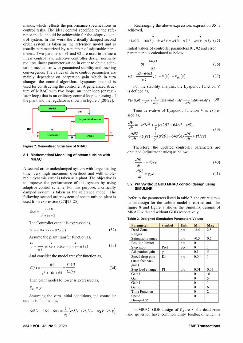
mands, which reflects the performance specifications in control tasks. The ideal control specified by the refe-rence model should be achievable for the adaptive con-trol system. In this work the critically damped second order system is taken as the reference model and is usually parameterized by a number of adjustable para-meters. Two parameters θ1 and θ2 are used to define a linear control law, adaptive controller design normally requires linear parameterization in order to obtain adap-tation mechanism with guaranteed stability and tracking convergence. The values of these control parameters are mainly dependent on adaptation gain which in turn changes the control algorithm. Lyapunov method is used for constructing the controller. A generalized struc-ture of MRAC with two loops: an inner loop (or regu-lator loop) that is an ordinary control loop consisting of the plant and the regulator is shown in figure 7 [20-22].

Model

Adjust mechanism

PlantController

Ym

α Y

uc

Figure 7. Generalised Structure of MRAC 3.1 Mathematical Modelling of steam turbine with

MRAC A second order underdamped system with large settling time, very high maximum overshoot and with intole-rable dynamic error is taken as a plant. The objective is to improve the performance of this system by using adaptive control scheme. For this purpose, a critically damped system is taken as the reference model. The following second order system of steam turbine plant is used from expression (27)[23-25].

1.2 8( )

2 6 8

sG s

ss

+=

+ +

The Controller output is expressed as,

)(2)(1 sysUCU θθ −= (32)

Assume the plant transfer function as,

)5421(3

1yyUcUcy αααα

α−

•−+

•=

•• (33)

And consider the model transfer function as,

64162

64)(

++=

sssG =

)(

)(

sUc

sym (34)

Then plant model follower is expressed as,

my y=

Assuming the zero initial conditions, the controller output is obtained as,

( )1 2 4 53

164 16 64C C CU y y U U y ya

α α α α− − = + − −

Rearranging the above expression, expression 35 is achieved,

yyUUyyU 5421364316364 ααααααα −•

−+•

=−•

− (35)

Initial values of controller parameters θ1, θ2 and error parameter e is calculated as below,

2

3641

α

αθ = (36)

( ) ( )m5 64 3

22

, e y s – y sα αθ

α−

= = (37)

For the stability analysis, the Lyapunov function V is defined as,

( ) 1 1 12 2 2, 1, 2 ( ( 2 2 64 3 5) ( 2 1 64 3)2 2 2

)V e eθ θ α θ α α α θ αα γ α γ

= + + − + − (38)

Time derivative of Lyapunov function V is expre-ssed as,

122 ( 2 2 64 3 5)

2 1 1( ) ( 2 1 64 3).( )

dV edtd dye Ucedt dt

α α θ α αγθ θγ α θ α γγ

= − + + − ⋅

⋅ − + − + (39)

Therefore, the updated controller parameters are obtained (adjustment rules) as below,

1d Ucedtθ γ= − (40)

2d yedtθ γ= (41)

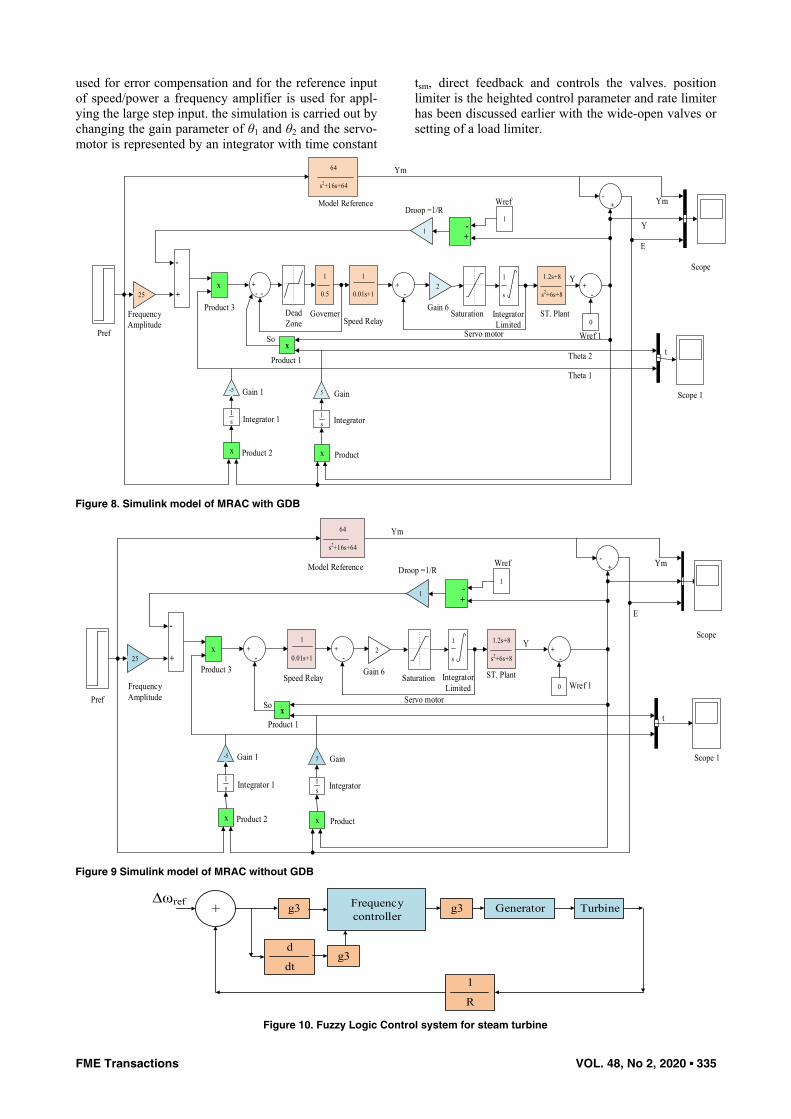
3.2 With/without GDB MRAC control design using SIMULINK

Refer to the parameters listed in table 2, the entire simu-lation design for the turbine model is carried out. The figure 8 and figure 9 shows the Simulink designs of MRAC with and without GDB respectively. Table 2. Designed Simulation Parameters Values

Parameter symbol Unit Min Max Dead Zone Ranges

p.u -2.5 2.5

Saturation ranges p.u -0.5 0.5 Position limiter p.u 0 1 Step input Pref Sec 0 1 Adaptation gain γ 0.1 5 Speed drop gain (state feedback gain)

KG p.u 0.04 1

Step load change Pl p.u 0.01 0.05 Gain1 0 -6 Gain 0 5 Gain4 0 1 Gain6 0 6 Time Function 0 2 Speed Droop=1/R

0 1

In MRAC GDB design of figure 8, the dead zone

and governor have common unity feedback, which is


used for error compensation and for the reference input of speed/power a frequency amplifier is used for appl-ying the large step input. the simulation is carried out by changing the gain parameter of θ1 and θ2 and the servo-motor is represented by an integrator with time constant

tsm, direct feedback and controls the valves. position limiter is the heighted control parameter and rate limiter has been discussed earlier with the wide-open valves or setting of a load limiter.

25

-

+x +

- -

1

0.01s+1+ -

21

s

1.2s+8

s2+6s+8+ -

0

-+

1

- +

64

s2+16s+64

1

x

1s

-5

x

1s

5

x

1

0.5

Pref

Frequency Amplitude

Product 3

GainGain 1

ProductProduct 2

IntegratorIntegrator 1

So

Product 1

Dead Zone

GovernerSpeed Relay

Gain 6Saturation Integrator

LimitedST. Plant

Servo motor

Wref

Wref 1

Ym

Ym

Y

E

Y

tTheta 2

Theta 1

Scope

Scope 1

Model ReferenceDroop =1/R

Figure 8. Simulink model of MRAC with GDB

25

-

+x +

-

1

0.01s+1+ -

21

s

1.2s+8

s2+6s+8+ -

0

-+

1

- +

64

s2+16s+64

1

x

1s

-5

x

1s

5

xPref

Frequency Amplitude

Product 3Speed Relay

Gain 6Saturation Integrator

LimitedST. Plant

Wref

Wref 1

Model Reference Droop =1/R

Ym

Ym

Y

E

So

Product 1

GainGain 1

ProductProduct 2

IntegratorIntegrator 1

Scope

Scope 1

Servo motor

t

Figure 9 Simulink model of MRAC without GDB

TurbineGeneratorFrequency controller

g3g3

g3

+∆ωref

d

dt1

R Figure 10. Fuzzy Logic Control system for steam turbine


+ -

-

+

100

dv/dt

51

0.5s

1

0.01s+1+ -

+ -

21

s

1.2s+8

s2+6s+8+ -

1

1

01

Droop =1/R

WrefWref

Step

AddGain 2

Derivative Saturation 1

Fuzzy Logic Controller

with Ruleviewer

Gain 3 Dead Zone

Governer

Feedback / Compensation

Speed Relay

Gain 6 Saturation Integrator Limited

Servo Motor

ST. Plant

PL

Scope

Y

Figure 11 Simulink model of Fuzzy Logic Control 4. PROPOSED FUZZY LOGIC CONTROLLER DESIGN USING SIMULINK

In the proposed design the input to the fuzzy logic controller is the error between the rotor inertial speed and reference speed. The rotor inertial speed rωΔ is multiplied with speed droop (1/R) and subtracted from reference speed refωΔ to yield the error. The error is fed to the fuzzy logic controller, shown in figure 10. The proposed model shown in figure 11. The design parameter is considered as the same from table2 used for the MRAC design [26]. 4.1 Fuzzy Membership functions for speed change

error (e) In this proposed fuzzy controller design, triangular fuz-zy membership function is chosen to control the steam turbine speed control, two inputs and one output vari-ables are proposed. It maps the values of fuzzy variables in a certain region to the degree of membership (μ) between 0 and 1. Input variable-1 is speed change error and input variable-2 is rate of change speed error. Output variable is change in valve position, the structure of fuzzy logic controller is mamdani type. Table 3. Fuzzy set and MFs for speed change error(e)

Fuzzy Set Range of MFs Membership function chosen

Low -50 to 0 OR 0 to 50 Triangular Normal/ medium

0 to 50 OR 50 to 100

Triangular

High 50 to 100 OR 100 to 150

Triangular

0

0 10 20 30 40 50 60 70 80 90 100

0.5

1

Mem

bers

hip

Func

tion

Low High

Normal

Speed Change Range Figure 12. Membership Function for speed change error (e)

Speed change is fuzzified into three triangular mem-bership functions and scaled in the range from -50 to 100 as shown in figure 12 and Table 3. The three MF of

speed change are Low, Normal and High, the value of -50 indicates that lowest speed change and the 100 indicates that highest speed change. 4.2 Fuzzy Membership functions for rate of change

of speed error (de/dt) Rate of change of Speed error is second variable inputs which is fuzzified into two triangular membership functions and scaled in the range from -30 to 30, as shown in figure 13 and Table 4. The two MF of rate of change of speed are Negative and Positive. The value of -30 indicates that lowest rate of change of speed and the value of 30 indicates that highest rate of change of speed. Triangular type of membership function produ-ced good result for the ranges of the variables considered. Table 4.Fuzzy set and MFs for input rate of change in speed error(de/dt)

Fuzzy Set

Range of MFs Membership function chosen

Negative -30 to -10 OR -10 to 10 Triangular Positive -10 to 10 OR 10 to 30 Triangular

0

-10 -8 -6 -4 -2 0 2 4 6 8 10

0.5

1

Mem

ber

ship

F

un

ctio

n

Nagtive Positive

Speed Change Range Figure 13. Membership Function for change in speed error (de/dt) 4.3 Fuzzy set and Membership Function for valve

position (output variable) The change in valve position is the output fuzzy vari-able which is evaluated for each bus by considering speed change error and rate of change of speed as input variables to the fuzzy expert system using a set of rules,


which are developed from qualitative descriptions. These rules are summarized in the fuzzy decision rule given in table 6, change in valve position is a fuzzy variable having five triangular membership functions and scaled in the range from -25 to 125, as shown in figure14 and Table 5. The five membership functions of change in valve position are Close Fast (CF), Close Slow(CS), No change(NC), Open slow (OS) and Open Fast (OF). The minimum value of change in valve position indicates the highest speed of the steam turbine.

The range for the MF was chosen based on the valve angle position opening percentage 100%,75%,50%,25% and 0% to show respectively, fully opened, almost fully opened, half opened, close slow and total closed posi-tion of valve. Table 5. Fuzzy set and MFs for valve position (output variable)

Fuzzy set Range of MFs Membership Function chosen

Close fast -25 to 0 OR 0 to 25 Triangular Close slow 0 to 25 OR 25 to 50 Triangular No change 25 to 50 OR 50 to 75 Triangular Open slow 50 to 75 OR 75 to 100 Triangular Open fast 75 to 100 OR 100 to 125 Triangular

0

0 10 20 30 40 50 60 70 80 90 100

0.5

1

Mem

ber

ship

F

un

ctio

n

Close F Ast

Normal

Speed Change Range

Close F Low Noc hangeClose F LowClose F Ast

Figure 14.Membership Function of valve position (the output variable)

4.4 Fuzzy Set Rule Base The design of the fuzzy controller essentially consists of choosing a set of rules (“rule base”), where each rule is based upon the knowledge that one has about the system. The following set of rules are designed which equi-valently shown in table 6 for the proposed design [27,28]. Table 6.Selection of Fuzzy Set Rule Base

Sl.No. Fuzzy Set Rule 1 If (Speed_change is Low) then (valve_position is

Open_fast) (1) 2 If (Speed_change is Normal) then (valve_position is

No_change) (1) 3 If (Speed_change is High) then (valve_position is

Close_fast) (1) 4 If (Speed_change is Normal) and (Rate is Positive)

then (valve_position is Close_slow) (1) 5 If (Speed_change is Normal) and (Rate is Negative)

then (valve_position is Open_slow) (1) 5. SIMULATION RESULTS 5.1 MRAC with/without GDB Control Design Simulation results are obtained and analysis is con-ducted using the developed model. Basic characteristics

and the effects on the stability were established. It can be observed that the characteristic of the plant with GDB is oscillatory with high value of overshoot and undershoot whereas the characteristic of the reference model is smooth without any oscillation. There is a large dynamic error between these two methods and that error has to be reduced to zero by using MRAC scheme. The adaptation gain ( ) is varied with a reference range from (0.1 to 5), it changes the values of control para-meters θ1 and θ2 respectively. These values of control parameters are used to improve the plant parameters.

(a)

(b)

Figure15.(a) Comparison between Reference speed, actual speed versus time for the system without GDB and Cont-roller. (b)Comparison between Reference speed, actual speed versus time for the system with GDB and without controller

Table 7. Time Response Specifications With and without Gdb For Different Adaptation Gain (From Figure 2, 3, 4 And 5)

Without any control With MRAC Without GDB Parameter With

GDB Without

GDB γ = 0.1 γ = 0.2 γ = 2 γ = 5 Peak

time(sec) 2.86 32.23 18.83 18.57 18.34 18.21

Maximum overshoot % 14.37 0.505 0.504 0.504 0.504 0.504

Undershoot % 3.23 1.97 1.875 1.92 1.94 1.97

Rise time(sec) 1.43 2.14 1.39 1.34 1.32 1.318

........ ......... -0.035 -0.063 -0.59 -1.49 ........... .......... 0.16 0.253 1.85 4.33

With MRAC With GDB γ = 0.1 γ = 0.2 γ = 2 γ = 5 19.66 19.47 19.2 19.24 0.505 0.505 0.505 0.505 1.913 1.99 1.86 1.96 1.972 1.967 1.965 1.964 -0.044 -0.089 -0.88 -2.2 0.2 0.37 3.114 7.53


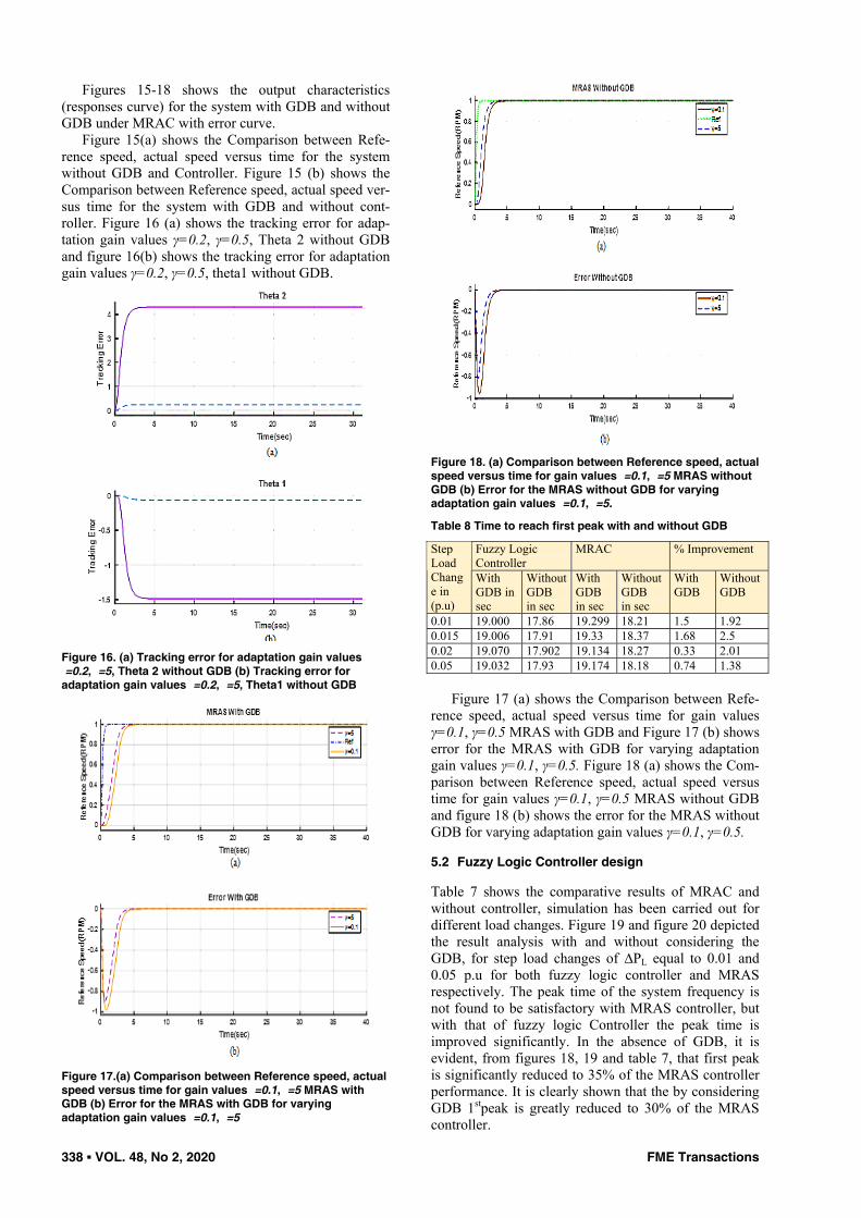
Figures 15-18 shows the output characteristics (responses curve) for the system with GDB and without GDB under MRAC with error curve.

Figure 15(a) shows the Comparison between Refe-rence speed, actual speed versus time for the system without GDB and Controller. Figure 15 (b) shows the Comparison between Reference speed, actual speed ver-sus time for the system with GDB and without cont-roller. Figure 16 (a) shows the tracking error for adap-tation gain values γ=0.2, γ=0.5, Theta 2 without GDB and figure 16(b) shows the tracking error for adaptation gain values γ=0.2, γ=0.5, theta1 without GDB.

Figure 16. (a) Tracking error for adaptation gain values �=0.2, �=5, Theta 2 without GDB (b) Tracking error for adaptation gain values �=0.2, �=5, Theta1 without GDB

Figure 17.(a) Comparison between Reference speed, actual speed versus time for gain values �=0.1, �=5 MRAS with GDB (b) Error for the MRAS with GDB for varying adaptation gain values �=0.1, �=5

Figure 18. (a) Comparison between Reference speed, actual speed versus time for gain values �=0.1, �=5 MRAS without GDB (b) Error for the MRAS without GDB for varying adaptation gain values �=0.1, �=5.

Table 8 Time to reach first peak with and without GDB

Fuzzy Logic Controller

MRAC % Improvement Step Load Change in (p.u)

With GDB in sec

Without GDB in sec

With GDB in sec

Without GDB in sec

With GDB

Without GDB

0.01 19.000 17.86 19.299 18.21 1.5 1.92 0.015 19.006 17.91 19.33 18.37 1.68 2.5 0.02 19.070 17.902 19.134 18.27 0.33 2.01 0.05 19.032 17.93 19.174 18.18 0.74 1.38

Figure 17 (a) shows the Comparison between Refe-rence speed, actual speed versus time for gain values γ=0.1, γ=0.5 MRAS with GDB and Figure 17 (b) shows error for the MRAS with GDB for varying adaptation gain values γ=0.1, γ=0.5. Figure 18 (a) shows the Com-parison between Reference speed, actual speed versus time for gain values γ=0.1, γ=0.5 MRAS without GDB and figure 18 (b) shows the error for the MRAS without GDB for varying adaptation gain values γ=0.1, γ=0.5. 5.2 Fuzzy Logic Controller design Table 7 shows the comparative results of MRAC and without controller, simulation has been carried out for different load changes. Figure 19 and figure 20 depicted the result analysis with and without considering the GDB, for step load changes of ∆PL equal to 0.01 and 0.05 p.u for both fuzzy logic controller and MRAS respectively. The peak time of the system frequency is not found to be satisfactory with MRAS controller, but with that of fuzzy logic Controller the peak time is improved significantly. In the absence of GDB, it is evident, from figures 18, 19 and table 7, that first peak is significantly reduced to 35% of the MRAS controller performance. It is clearly shown that the by considering GDB 1stpeak is greatly reduced to 30% of the MRAS controller.


The comparative result of fuzzy logic Controller and MRAS controller with and without GDB is given in table 8, from the tabulated results, it is evident that the fuzzy logic controller performance is better over the MRAS controller.

Figure 19.(a) Comparison between Reference speed deviation , actual speed deviation versus time with FLC for the step load change �Pl =0.01, and 0.05 p.u with GDB (b) Comparison between Reference speed deviation , actual speed deviation versus time with FLC for the step load change �Pl =0.01, and 0.05 p.u without GDB

Figure 20.(a) Comparison between Reference speed deviation , actual speed deviation versus time with MRAS for the step load change �Pl =0.01, and 0.05 p.u with GDB (b) Comparison between Reference speed deviation , actual speed deviation versus time with MRAS for the step load change �Pl =0.01, and 0.05 p.u without GDB

5.3 Comparative analysis of MRAC and FLC

The comparative results analysis is made with reference MRAC and FL controllers shown in figure 21 and 22. It infer from these results that the steam turbine speed control is more responsive to FL controller than to MRAC for both when GDB is present and absent. It attribute this to the simplicity and quick adaptability of FL controller as compared with MRAC.

Figure 21. Comparison between Reference speed, actual speed versus time and MRAS, FL controller without governor GDB

Figure 22. Comparison between Reference speed, actual speed versus time and MRAS, FL controller without governor GDB 6. CONCLUSION A Fuzzy and MRAS Controllers are proposed to be ana-lysed comparatively. A detailed comparison between these techniques has been carried out. The simulation has demonstrated that without any control under inclu-sion of GDB and without GDB, with both conditions the plant performance is very poor with very high values of overshoot and undershoot. However, the application of MRAC by using Lyapunov stability theory reduces the value of overshoot and undershoot specially for plant without GDB.

The increment in adaptation gain both the peak time and rise time for the case with and without GDB decre-ases. Also, the control parameters vary in the direction to improve system performance with the increment in adaptation gain. But beyond the chosen range of adap-


tation gain (0.1 ≤ γ ≤ 5), the system performance is very poor for both the case without any controller and MRAC. The system may even become unstable for the wrong choice of adaptation gain. Therefore, it is shown that for suitable values of adaptation gain, the Lyapunov stability theory makes the plant output as close as possible to reference model in MRAC comparing to the case of without any controller. But comparing the MRAC with the fuzzy logic controller using step input, the time to reach first peak with GDB is 19.00s and without GDB for fuzzy logic is 17.86s and 19.29s with and 18.21s without GDB for MRAC. This can be 1.5% with GDB and 1.92% without GDB improvement bet-ween fuzzy and MRAC, so based on the findings presented in the earlier discussion(table7), proposed fuzzy logic controller response is more satisfactory.

REFERENCES

[1] Nandini Priyanka G, Ishwarya S, Janaki Raman S, Thana Sekar C, Vaishali P “Design of model refe-rence adaptive controller for cylinder tank system”, International Journal of Pure and Applied Mathe-matics, Volume 118 No. 20, 2007-2013 ISSN: 1311-8080 (printed version); ISSN: 1314-3395 (on-line version), 2018.

[2] Mohamed. M. Ismail, “Adaptation of PID cont-roller using AI techniques for speed control of iso-lated steam turbine,” IEEE Journal of Control, Automation and Systems, vol. 1, no. 1,2012.

[3] S.B.M. Ibrahim, “The PID controller design using genetic algorithm”, University of Southern Queens land Research Project, October, 2005

[4] Ahmed Rubaai, “Developed the DSP-Based Laboratory model of Hybrid Fuzzy-PID Controller Using Genetic optimization for high-performance Motor Drives”, IEEE Industry Applications Nov, 2008

[5] Mohamed.M. Ismail, “Neuro fuzzy controller (ANFIS) for Speed Control of Isolated Steam Turbine”, IEEE Journal of Control, Automation and Systems, 2013.

[6] Sanjay Kr. Singh, “Multi-objective optimization of the PID controllers for optimal speed control for an isolated steam turbine”, journal of applied Science, Engineering and Technology 7(17), May, 2014.

[7] Bennauer M et al., “Automation and control of electric power generation and distribution system: steam turbine”, Encyclopaedia of Life Support Systems, Vol. XVIII; 2012.

[8] Quatrano A.a, De Simone M.C.a, Rivera Z.B.b, Guida D.a , Development and implementation of a control system for a retrofitted CNC machine by using Arduino, FME Transactions 2017, vol. 45, iss. 4, pp. 565-571.

[9] Shoga T, Thelkar A, Bharatiraja C, Mitiku S, Adedayo Y. Self-tuning regulator based cascade control for temperature of exothermic stirred tank reactor, FME Transactions; 2019;47(1):202–11.

[10] Kasilingam F, Pasupuleti J, Bharatiraja C, Adedayo Y. Power system stabilizer optimization using BBO

algorithm for a better damping of rotor oscillations owing to small disturbances, FME Transactions; 2019;47(1):166–76.

[11] Jagadeesh Pasupuleti, C Bharatiraja, Yusuff Adedayo, Single Machine Connected Infinite Bus System Tuning Coordination Control using Biogeo-graphy-Based Optimization Algorithm, FME Transactions; 2019;47(3):503-510.

[12] M. Maeda and S. Murakami, “A self-tuning fuzzy controller, Fuzzy Sets and Systems”, vol.51, pp. 29-40, 1992.

[13] Y. Wang , et al: “Model and Nonlinear Analysis of 300MW Steam Turbine Speed Control System,” Steam Turbine Technology, Vol. 49, No. 1, pp. 17-20,2007.

[14] Chaibakhsh A et al., “Simulation modelling practice and theory”, pp. 1145–1162, 2008.

[15] Andrea Cristofaro, Sergio Galeani, Simona Onori, Luca Zaccarianf,, “A switched and scheduled design for model recovery anti-windup of linear plants”, Preprint submitted to European Journal of Control April 10, 2018.

[16] Lukáš Hubka, Petr Školník, “Steam turbine and steam reheating simulation model”, IEEE Interna-tional Conference on Process Control (PC), pp. 31–36, June 2013.

[17] Suttipan Limanond, Kostas S. Tsakalis, “Model Reference Adaptive and Non-Adaptive Control of Linear Time-Varying Plants”, IEEE Transactions on Automatic Control, Vol. 45(7), pp. 1290-1300, July 2000.

[18] Sun, Meng, “A single neuron PID controller based PMSM DTC drive system fed by fault tolerant 4-switch 3-phase inverter”, IEEE International Conference on Industrial Electronics and Applications,2006

[19] Ioannis Baltas, Anastasios Xepapadeas, Athanasios N. Yannacopoulos, “Robust control of parabolic stochastic partial differential equations under model uncertainty”, Preprint submitted to Elsevier May 4, 2018

[20] T. John Koo, “Stable Model Reference Adaptive Fuzzy Control of a Class of Nonlinear Systems”, IEEE Transactions on Fuzzy Systems, Vol. 9, No. 4, pp. 624 – 636, 2001.

[21] Torbj¨orn Wigren, “A disturbance rejection and data rate trade-off in networked data flow control”, Preprint submitted to European Journal of Control July 6, 2018.

[22] A.M. Zou, Z. G. Hou, M. Tan, “Adaptive Control of a Class of Nonlinear Pure-Feedback Systems Using Fuzzy Backstepping Approach”, IEEE Trans. Fuzzy Syst., vol. 16, no.4, pp. 886-897, 2008.

[23] M. Hojati, S. Gazor, “Hybrid adaptive fuzzy iden-tification and control of nonlinear systems”, IEEE Trans. Fuzzy Syst., vol. 10, no.2, pp. 198-210, 2002.

[24] Chun-Yao Chen, Chin-Ming Hong and Yih-Guang Leu, “Nonlinear Parameter Fuzzy Control for


Uncertain Systems with Only System Output Measurement”, FUZZ-IEEE korea, August 20-24,2009.

[25] Dettori S, Iannino, V, Colla V, Signorini A, “A fuzzy-logic based tuning approaches of PID control for steam turbines for solar applications”, Energy Procedia, 105, 480–485, 2017.

[26] Mier D. et al.: “Model predictive control of the steam cycle in a solar power plant”, IFAC-Papers on Line, 48, 710–715, 2015.

[27] Pourbeik, P. “Dynamic models for turbine-governors in power system studies”, IEEE Task Force Report on Turbine Governor Modelling, IEEE Power & Energy Society: Piscataway, NJ, USA, 2013.

[28] Mr. Chetan M. Rajgire, Miss Mona N. Wankhede, Mr. Sushil S. Karvekar, “Design and Implemen-tation of Sensor less Vector Control of Induction Motor Drive using Fuzzy Adaptive Controller”, Proceedings of the IEEE, International Conference on Computing Methodologies and Communication (ICCMC), 2017.

NOMENCLATURE

FHP High pressure turbine power fraction FMP Medium pressure turbine power fraction FLP Low pressure turbine power fraction TLH Reheat time constant THP Steam Chest time constant TLP Crossover piping time constant TSM Valve positioner time constant Tg Governor time constant γ Adaptation gain

KG Speed drop gain (state feedback gain) Tsr Speed Relay time constant GHP High pressure transfer function GMP Medium pressure transfer function GLP Low pressure transfer function ΔPGV Change in Steam valve position ΔPm Change in mechanical power θ1, θ2 Controller parameters

РЕФЕРЕНТНИ ДИЗАЈН И КОМПАРАТИВНА АНАЛИЗА АДАПТИВНОГ УПРАВЉАЊА НА БАЗИ РЕФЕРЕНТНОГ МОДЕЛА КОД

УПРАВЉАЊА БРЗИНОМ ПАРНЕ ТУРБИНЕ

А. Фејо, А.Р. Телкар, Ц. Бхаратираџа, Ј. Адедајо

Приказује се математичко моделирање склопа парне турбине са фази контролером у изолованим радним условима, нарочито у нуклеарним електранама. Ниво воде у парном генератору је један од главних узрока искључења реактора. Овај проблем је пос-ледњих година постао актуелан јер парни генератор и контрола брзине управљања представљају нели-неарни систем који показује инверзну динамику одзива. Дизајниран је SIMULINK модел турбине са фази контролером. Резултати су упоређени и анализирани техником МRAC дизајна да би се нашло боље методолошко решење контроле брзине код парне турбине и постигло ефективно време адаптације од 0,3 до 2,5% са и без GDB. Побољшање праћења задате тачке и контрола брзине турбине по времену приказана је за случајеве у присуству и одсуству промене опсега улазне величине.

Reference Design and Comparative Analysis of Model ...

Documents

Transcript of Reference Design and Comparative Analysis of Model ...