Redundancy and Coverage Detection in Sensor …younis/Sensor_Networks/...Redundancy and Coverage...

Redundancy and Coverage Detection inSensor Networks

BOGDAN CARBUNAR, ANANTH GRAMA, and JAN VITEK

Purdue University

and

OCTAVIAN CARBUNAR

IFIN-NIPNE

We study the problem of detecting and eliminating redundancy in a sensor network with a view

to improving energy efficiency, while preserving the network’s coverage. We also examine the im-

pact of redundancy elimination on the related problem of coverage-boundary detection. We reduce

both problems to the computation of Voronoi diagrams, prove and achieve lower bounds on the

solution of these problems, and present efficient distributed algorithms for computing and main-

taining solutions in cases of sensor failures or insertion of new sensors. We prove the correctness

and termination properties of our distributed algorithms, and analytically characterize the time

complexity and traffic generated by our algorithms. Using detailed simulations, we also quantify

the impact of system parameters such as sensor density, transmission range, and failure rates on

network traffic.

Categories and Subject Descriptors: C.2.1 [Computer-Communication Networks]: Network

Architecture and Design—Distributed networks, Network topology; C.2.4 [Computer-Communication Networks]: Distributed Systems—Distributed applications

General Terms: Algorithms, Design

Additional Key Words and Phrases: Sensor networks, coverage, energy efficiency, redundancy elim-

ination, coverage boundary

1. INTRODUCTION

The need for distributed sensing and monitoring of remote or inaccessibleareas, along with the integration of sensed information into a variety ofphysical processes provides overarching motivations for sensor networks.The emphasis on low-cost, dense sensing comes with significant constraints

This work was funded in part by NSF grants CCF 0325227, CCF 0444285, and CMS 0443148. A

preliminary version of this work was presented at IEEE SECON 2004.

Authors’ addresses: B. Carbunar, A. Grama, J. Vitek, Computer Science Department, Purdue Uni-

versity, West Lafayette, IN, 47906; email: {carbunar,ayg,jv}@cs.purdue.edu; O. Carbunar, IFIN-

NIPNE, Magurele, Romania; email: [email protected].

Permission to make digital or hard copies of part or all of this work for personal or classroom use is

granted without fee provided that copies are not made or distributed for profit or direct commercial

advantage and that copies show this notice on the first page or initial screen of a display along

with the full citation. Copyrights for components of this work owned by others than ACM must be

honored. Abstracting with credit is permitted. To copy otherwise, to republish, to post on servers,

to redistribute to lists, or to use any component of this work in other works requires prior specific

permission and/or a fee. Permissions may be requested from Publications Dept., ACM, Inc., 1515

Broadway, New York, NY 10036 USA, fax: +1 (212) 869-0481, or [email protected]© 2006 ACM 1550-4859/06/0200-0094 $5.00

ACM Transactions on Sensor Networks, Vol. 2, No. 1, February 2006, Pages 94–128.

Redundancy and Coverage Detection in Sensor Networks • 95

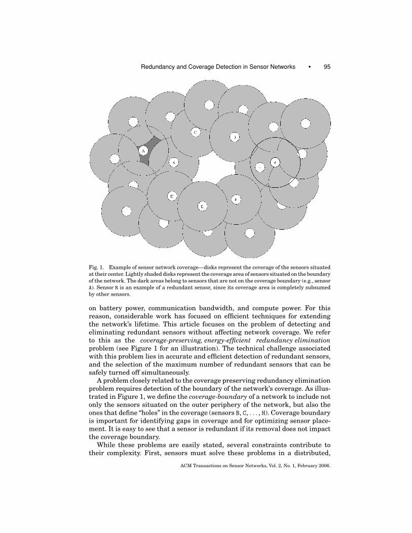
Fig. 1. Example of sensor network coverage—disks represent the coverage of the sensors situated

at their center. Lightly shaded disks represent the coverage area of sensors situated on the boundary

of the network. The dark areas belong to sensors that are not on the coverage boundary (e.g., sensor

A). Sensor R is an example of a redundant sensor, since its coverage area is completely subsumed

by other sensors.

on battery power, communication bandwidth, and compute power. For thisreason, considerable work has focused on efficient techniques for extendingthe network’s lifetime. This article focuses on the problem of detecting andeliminating redundant sensors without affecting network coverage. We referto this as the coverage-preserving, energy-efficient redundancy eliminationproblem (see Figure 1 for an illustration). The technical challenge associatedwith this problem lies in accurate and efficient detection of redundant sensors,and the selection of the maximum number of redundant sensors that can besafely turned off simultaneously.

A problem closely related to the coverage preserving redundancy eliminationproblem requires detection of the boundary of the network’s coverage. As illus-trated in Figure 1, we define the coverage-boundary of a network to include notonly the sensors situated on the outer periphery of the network, but also theones that define “holes” in the coverage (sensors B, C, . . . , H). Coverage boundaryis important for identifying gaps in coverage and for optimizing sensor place-ment. It is easy to see that a sensor is redundant if its removal does not impactthe coverage boundary.

While these problems are easily stated, several constraints contribute totheir complexity. First, sensors must solve these problems in a distributed,

ACM Transactions on Sensor Networks, Vol. 2, No. 1, February 2006.

96 • B. Carbunar et al.

efficient, and scalable manner. Second, solutions to these problems must beadaptive in nature when old sensors fail or new ones are deployed, the newsolution must be rapidly computed from the previous solution. Finally, sinceRF interfaces have a limited transmission range, protocols must account foroverheads of multihop routing. Since communication typically consumes moreenergy than computation, the protocols themselves need to be energy efficient.

The idea of turning off selected sensors in order to extend the lifetime of thenetwork has been previously explored. Zhang and Hou [2004] propose OGDC, adistributed algorithm, which works on the principle that an area is completelycovered by a set of sensors if the crossing points generated by the sensingdisks are covered. While OGDC’s purpose is to minimize the number of sen-sors covering the crossing points, it declares as redundant only those sensorswhose bitmapped sensing disks are completely covered by their transmissionneighbors. Wang et al. [2003] propose a protocol, CCP, based on a similar ob-servation. However, the complexity of determining the redundancy of a sensoris O(N3), where N is the number of sensors within twice the sensing range ofthat sensor. Huang and Tseng [2003] propose an algorithm for determining thek-coverage of a region by a sensor network, based on the notion of k-perimeter-coverage. As with OGDC [Zhang and Hou 2004] and CCP [Wang et al. 2003]each sensor computes its k-coverage by communicating with all the sensorswithin twice its sensing range. The computational complexity of the methodis O(N log N). However, in order for a sensor s to determine its redundancy, ithas to ask all the sensors within twice its sensing range to reevaluate theirperimeter coverage without s. Thus, for each sensor, the actual complexity ofdetermining its redundancy is O(N2 log N). Tian and Georganas [2002] declare asredundant, sensors whose transmission neighbors completely “sponsor” theirsensing disks. Thus, the algorithm is completely localized. Ye et al. [2003] pro-pose a randomized algorithm for turning off sensors, whose primary goal is notto maintain coverage.

In contrast to these existing results, we present a more efficient deterministicsolution to the problem of accurately detecting redundant sensors and safely(from a coverage standpoint) turning them off. The complexity of our solutionfor each sensor s is O(N log N), where N is the number of Voronoi neighbors ofs. We also present efficient algorithms for maintaining the solution in casesof sensor failures and new sensor deployments. We show that the expectednumber of sensors affected is O(log N). Moreover, since our solution relies onVoronoi diagrams, a sensor affected by a new or a failing sensor can recomputeits redundancy in O(log N) expected time [Devillers et al. 1992], whereas thesolutions of Zhang and Hou [2004] and Wang et al. [2003] require O(N3) and thesolution of Huang and Tseng [2003] requires O(N2 log N).

While our work focuses on extending the coverage lifetime of wireless sensornetworks, prior work [Zhang and Hou 2004; Wang et al. 2003] has explored therelationship between coverage and connectivity of sensor networks. Specifically,both Zhang and Hou [2004] and Wang et al. [2003] prove that if the transmissionrange of sensors equals or exceeds twice their sensing range, coverage impliesconnectivity. Moreover, the work of Wang et al. [2003] extends this result fork-coverage and k-connectivity. The results presented in this article, however,



are not based on assumptions regarding the relationship between sensing andtransmission ranges of sensors.

This article makes the following specific contributions: in Section 4, we derivenecessary and sufficient conditions for a sensor to be redundant and presentan efficient distributed algorithm for the coverage-preserving, energy-efficientredundancy elimination problem. In Section 5, we present necessary and suffi-cient conditions for a sensor to be on the coverage boundary. We prove a lowerbound of �(n log n) for any (serial) algorithm for the problem, where n is thetotal number of sensors in the network. We present a distributed algorithm forcomputing the coverage-boundary, whose serial counterpart has �(n log n) com-plexity. Both algorithms are based on the distributed and adaptive constructionof Voronoi diagrams. In Section 6, we present efficient and scalable distributedalgorithms for recomputing local Voronoi information in the event of sensor fail-ures and deployment of new sensors. The algorithms are then used to efficientlymaintain the redundancy and coverage-boundary information, without recom-puting the entire solution. We show that our algorithms are efficient and provetheir correctness and stability. In Section 7, we experimentally characterize theperformance of our algorithms, and conclusions are drawn in Section 8.

2. RELATED RESEARCH

The problem of coverage of a set of entities has been studied in a variety ofcontexts. Zhang and Hou [2004] prove the interesting result that if the trans-mission range of sensors equals or exceeds twice the sensing range, coverageimplies connectivity of the sensor network. Furthermore, they prove that, givena region R containing sensors, if each crossing point (intersection point of sens-ing disks of sensors) in R is covered by at least one other sensor in R, then R iscompletely covered by the sensors. Based on this result, they propose OGDC, adistributed algorithm for selecting a subset of the sensors covering all crossingpoints. The selected sensors need to stay active, while the rest can be turnedoff. During the decision stage, each sensor can be in one of the following states:UNDECIDED, ON, and OFF. A sensor switches to OFF only when its sensingdisk is completely covered by its neighbors. To verify this condition, the sensingdisk is divided into small grids and a bitmap is used to indicate whether thecenter of each grid is covered by a neighbor of the sensor.

Wang et al. [2003] prove a result regarding the connection between cover-age and connectivity similar to Zhang and Hou [2004] and extend the resultto the case of k-coverage implying k-connectivity. Specifically, they prove thatif the transmission range is larger than or equal to, the sensing range of sen-sors, k-coverage implies k-connectivity of the network and 2k-connectivity ofthe interior of the network. They also prove that if all crossing points in thedeployment area are k-covered the area is k-covered. Based on this result, theypropose a distributed algorithm for turning off redundant sensors. A sensor s1decides to be inactive if all the crossing points inside its sensing range are atleast k-covered. The time complexity of this decision algorithm is O(N3), whereN is the number of sensors within the distance of twice the sensing range of s1.In comparison, the corresponding complexity of our algorithm is only O(N log N)



(the time required to build the Voronoi diagram of the sensors placed withintwice the sensing range of s1).

Tian and Georganas [2002] present an algorithm for detecting sensors whosecoverage area is completely covered by other sensors. A sensor s1 turns itself offonly when each sector of its sensing disk is covered by one of the sensors locatedinside its sensing range. If s2 is such a sensor, the algorithm conservativelyconsiders only the sector generated by the intersection of the sensing disks ofs1 and s2 to be “sponsored” by s2. In contrast, our solution considers the entire“lune” of s1, generated by the intersection of the sensing disks of s1 and s2, tobe covered by s2. Jiang and Dou [2004] identified several shortcomings of Tianand Georganas [2002] and provided a protocol for improving its performance.

Huang and Tseng [2003] propose an algorithm for determining the k-coverage of a region by a sensor network. They prove that an area is k-covered ifeach sensor in the network is k-perimeter-covered, where a k-perimeter-coveredsensor has each point on the perimeter of its sensing disk covered by at leastk other sensors. Note that a 1-perimeter-covered sensor is equivalent to a noncoverage-boundary sensor, as defined in Section 5. The solution for determiningperimeter coverage requires each sensor to communicate with all the sensorswithin twice its sensing range N—its computational complexity is O(N log N).Their solution is then used to determine redundancy and schedule inactive pe-riods for redundant sensors. However, to determine its redundancy, a sensors has to ask all the sensors within twice its sensing range to reevaluate thecoverage of their perimeter without s. Thus, a sensor has to run the perimetercoverage N times, making the complexity of the protocol O(N2 log N).

The solutions we propose improve on the results of the above works by al-lowing a sensor to determine its redundancy and presence on the coverage-boundary, while communicating only with its Voronoi neighbors. If the numberof Voronoi neighbors of a sensor is N, the computation complexity of our protocolsis O(N log N). Moreover, we provide efficient algorithms that distributively main-tain the redundancy and coverage-boundary information when existing sensorsfail and new sensors are deployed. For each sensor failure or new sensor de-ployment, the expected number of sensors affected by the notifications sent inour algorithms is only O(log N). Moreover, the operation of updating the localinformation based on such a notification has an expected complexity of O(log N).

Ye et al. [2003] present a randomized algorithm for extending the networklifetime by keeping only a subset of the sensors active at any given time. Ini-tially each sensor sleeps for a duration distributed according to an exponentialdistribution function λe−λt, where λ is the average rate of probing. When a sen-sor s1 wakes up, it queries other sensors placed within its probing range, Rp.If at least one other sensor answers, s1 turns back to sleep for a duration thatis distributed according to an exponential distribution function. Otherwise, itbecomes active for the remainder of its life. While the probing range is ad-justable, enabling control of the sensor network’s node density, the algorithmcannot guarantee complete coverage. This article proves, however, that if thetransmission range of sensors equals or exceeds (1 + √

5)Rp, and each squarecell of size Rp contains at least one sensor, then the active network of PEAS isconnected with high probability.



Slijepcevic and Potkonjak [2001] introduce a centralized algorithm for find-ing the maximum number of disjoint subsets of sensors, or covers, where eachcover completely covers the same area as the initial set of sensors. They provethe problem to be NP-complete. Their solution is based on building sets ofmonitored points into disjoint fields, such that each field contains a maximumnumber of points covered by the same sensors. At each stage, a cover is built ina greedy fashion by associating an objective function with sensors that cover afield. The objective function gives the likelihood of generating redundant cov-ers. Initially, a critical field, one covered by the smallest number of sensors, isselected. Then, the sensor that covers the field and has the highest objectivefunction is selected. Selected fields and sensors are marked accordingly, andthis process is repeated until a full cover is obtained.

Gupta et al. [2003] use the notion of field defined above to provide central-ized and distributed algorithms for computing connected sensor covers for queryregions. Initially, a sensor in the query region is selected. A candidate set of sen-sors, whose sensing disks intersect the sensing disks of selected sensors is built.For each candidate sensor, a path from it to one selected sensor is constructed.The candidate sensor, along with its path, which covers the maximum numberof uncovered fields is selected. In the proposed distributed version of this algo-rithm, this computation is performed by the last selected sensor. Furthermore,the search for the candidate sensor is done within a radius of 2r, where r is themaximum distance between any two sensors whose sensing disks overlap.

Carle and Simplot-Ryl [2004] extend the protocol of Dai and Wu [2003], pro-viding connected dominating sets of nodes in ad hoc networks, to constructarea-dominating sets of sensor networks. In this protocol, sensors listen for atimeout period, for advertisements containing decisions of their neighbors be-fore deciding their own state. When the timeout expires, a sensor checks thatthe subgraph of the neighbors that have sent advertisements is connected, andthat those neighbors completely cover its sensing disk. If this is the case, thesensor sends a positive advertisement to its neighbors. Otherwise, it has theoption to transmit a negative advertisement or not.

Meguerdichian et al. [2001] define the coverage using the best covered andleast covered paths between two sensors in the network as metrics. Haas [1997]presents algorithms for optimizing coverage under constraints on message pathlength. Shakkottai et al. [2003] study the coverage of a unit square by a givennumber of sensors, under the assumption that sensor failures will affect thecoverage. We refer readers to Cardei and Wu [2004] for an extensive survey ofcoverage problems in sensor networks.

The problem of sensor coverage has also received considerable attention inrobotics (please see Choset [2001] for a survey). Given a bounded domain, theproblem requires a robot equipped with a sensor to build a complete map ofthe environment without any initial knowledge. This requires the robot to passthrough specified points of the unknown region. The notion of a hierarchicalgeneralized Voronoi graph is used to incrementally construct the map usingonly line of sight data.

Distributed computation of Voronoi diagrams is addressed in Stojmenovic[1999] in the context of routing in ad hoc networks and in Hu [1993] in the



Fig. 2. Voronoi diagram of the sensors in Figure 1. The circles represent the coverage disks of the

labeled sensors. Note that the coverage area completely covers their Voronoi cell only for A and R.

In the next section we will show that this is not a coincidence.

context of topology control of ad hoc networks. In this approach, a sensor buildsa Voronoi diagram of itself and its neighbors. While these protocols are localized,they provide an approximation of the actual Voronoi cells of sensors and canproduce false negatives for the problems addressed in this article.

3. OVERVIEW OF VORONOI TESSELLATIONS

Given a set S of n sites s1, s2, .., sn in a plane, their Voronoi diagram is definedas the subdivision of the plane into n cells, one for each site, with the propertythat any point in the cell corresponding to a site is closer to that site than toany other site. Formally, the Voronoi cell corresponding to site si is defined as

cellvd(si) =n⋂

j=1,j �=i

{x|dist(si, x) ≤ dist(sj, x)}.

We use the notation dist(p, q) to denote the Euclidean distance between twopoints p and q. Two Voronoi cells meet along a Voronoi edge, and three Voronoicells meet at a Voronoi vertex. We call a site a neighbor of another site ifthe Voronoi cells of the two sites share an edge. We use these two termsinterchangeably. Figure 2 illustrates the Voronoi diagram of the network inFigure 1.

A Delaunay triangulation of a set S of sites is defined as the unique triangu-lation of S such that no point in S is inside the circumcircle of any triangle of thetriangulation. A Delaunay triangulation is the dual of the Voronoi diagram ofS, in the sense that two sites are vertices of the same Delaunay triangle if and



only if they are Voronoi neighbors. We formally define the Delaunay distanceas follows:

Definition 3.1. The Delaunay distance between two sites is the minimumnumber of hops on the Delaunay graph between the two sites.

For example, in Figure 2, sensors A and R are at Delaunay distance 4.

Multiplicative Weighted Voronoi Diagram A Multiplicative WeightedVoronoi Diagram (MWVD) is defined in a manner similar to a Voronoi diagram,with the addition of weights at each of the n sites. In the definition of theclassical Voronoi diagram, the sites have equal weights. The MWVD replacesthe Euclidean distance used by the Voronoi diagram with a new distance dmvdefined by

dmv(si, x) = dist(si, x)

wi. (1)

In this definition, si corresponds to one of the n sites in the plane, wi isa weight associated with it, dist is the Euclidean distance function, and xcorresponds to any point in the plane. The Multiplicative Weighted Voronoi cellof each site is formally defined as follows:

cellmwvd(si) =n⋂

j=1,j �=i

{x|dmv(si, x) ≤ dmv(sj, x)}.

4. ENERGY-EFFICIENT COVERAGE

In this section we formalize the coverage-preserving energy efficient redundantsensor elimination problem, and provide a solution, RSE, based on Voronoi tes-sellations. We make the assumption that each sensor knows its two dimen-sional location. This is a reasonable assumption since, in the absence of thisinformation, the coverage-boundary and the redundancy information cannot beuniquely or correctly determined (from topological information alone). Whileinitially we assume that all the sensors in the network have the same sensingrange, in Section 4.1 we extend our results to heterogeneous sensor networks,using multiplicative weighted Voronoi diagrams.

Definition 4.1. The coverage of a sensor s with planar coordinates (x, y)and sensing range r is a disk with center (x, y) and radius r. We call thisdisk the coverage or sensing disk, and call its border the coverage or sensingcircumcircle, denoted by C(s). We say that a point p is covered by a sensor s ifdist(s, p) ≤ r.

The coverage of a network is the union of the coverage disks of all the sensorsin the network. Formally, we have:

Definition 4.2. The coverage of a network is the area A with the propertythat for any point p ∈ A, there exists at least one sensor s in the network suchthat p is covered by the coverage disk of s.

The definition of a redundant sensor follows naturally:



Fig. 3. Multiplicative weighted Voronoi diagram (MWVD) of 20 sensors. Each sensor is represented

by a point, and its weight, determining the size of its cell.

Definition 4.3. A sensor is said to be redundant if its sensing area iscompletely covered by other sensors.

We define the 2-Voronoi diagram of a sensor in the following manner:

Definition 4.4. The 2-Voronoi diagram of a sensor s is the Voronoi diagramof the Voronoi neighbors of s, when s is excluded. The 2-Voronoi Vertices (2-VV)of a sensor s are the Voronoi vertices of the 2-Voronoi diagram of s. A 2-VoronoiIntersection Point (2-VIP) of s is the intersection between an edge of the 2-Voronoi diagram and the coverage circumcircle of s. A 2-Voronoi edge (2-VE)of s is either a Voronoi edge between 2-Viv’s of s, or a Voronoi edge between a2-VV and a 2-VIP of s.

Figure 4 illustrates an example of a redundant sensor. In this example, sen-sor s1 has five 2-VEs, one between two 2-VVs, 2 − V1 and 2 − V2, and the restbetween a 2-VV and a 2-VIP of s1.



Fig. 4. Example redundant sensor, s1. Points 2 − V1 and 2 − V2 are 2-VVs of s1, and 2 − VIP1..4 are

2-Voronoi Intersection Points of s1. Note that 2 − V1,2 and 2 − VIP1..4 are all covered by at least two

of the Voronoi neighbors of s1.

In the following, we use Ns to denote the set of sensors that are the Voronoineighbors of a sensor s. The following lemma shows an important property ofthe coverage of Voronoi neighbors.

LEMMA 4.1. For any sensor s in the network, the sensors in Ns are the onesclosest to s, out of all the sensors in the network. More precisely, if a sensor thatis not in Ns covers a point p inside the coverage disk of s, then p is also coveredby at least one sensor in Ns.

PROOF. Let us consider the case in which sensor s1 has neighbors s2, ands3 whose coverage areas intersect each other and also the coverage area ofs1 (Figure 5). We assume that all the sensors have the same coverage range,r (recall that this assumption can be relaxed with the use of MWVDs as op-posed to Voronoi diagrams). Let v be the Voronoi vertex generated by thethree sensors. Figure 5 also shows the circumcircle of sensors s1, s2 and s3,centered at v, containing no other sensor. Let e be the intersection point be-tween this circle and the Voronoi edge generated by s2 and s3. The only area



Fig. 5. Proof of Lemma 4.1. If sensors s1, s2, and s3 are mutual Voronoi neighbors, another sensor

can only be placed in the hashed area. Otherwise, that sensor would be a Voronoi neighbor of s1.

where another sensor, that is not a Voronoi neighbor of s1, can be placed, is thehashed area. Observe that dist(b, e) = dist(b, v) + dist(v, e). Therefore, due totriangle inequality, dist(b, e) = dist(b, v) + dist(s3, v) > dist(s3, b) = r. Also,dist(s2, a) = dist(s2, b) = r. It is easy to prove then, that the distance betweenany point on the arc ab and a point on the arc s2e is greater than or equal to r.The arcs are emphasized in Figure 5. Similarly, the distance between any pointon the arc bc and any point on the arc s3e is greater than or equal to r. Hence,any sensor placed in the hashed area covers less of s1’s coverage area than s2and s3. The cases where the coverage areas of s2 and s3 do not intersect, or donot intersect the coverage area of s1 can be similarly proved.

The following theorem, the main result of this section, translates the problemof finding a redundant sensor to a local examination of the sensor’s Voronoineighbors.

THEOREM 4.1. A sensor s is redundant if and only if all the 2-VVs and 2-VIPsof s are covered by the Voronoi neighbors of s.

PROOF. If a sensor s is redundant, then all its 2-VVs and 2-VIPs are cov-ered by the Voronoi neighbors of s. This is illustrated in Figure 4, which showsan example of a redundant sensor, s1. Since the coverage area of s1 is com-pletely covered by other sensors, using Lemma 4.1, we infer that it is completely



covered by the Voronoi neighbors of s1. Furthermore, since the coverage area ofa sensor is a circle, any three neighbors of s1 that are mutual neighbors whens1 is excluded, will cover a common area. Figure 4 shows the common areas ofVoronoi neighbors s2, s4, and s5, and s2, s3, and s4, respectively, as the hashedareas. The common area of such three-neighbor sets contains the Voronoi vertexgenerated by them. This Voronoi vertex is a 2-VV of s1, and is therefore coveredby three Voronoi neighbors of s1. In a similar fashion it can be proved that each2-VIP of s1 is covered by at least two of the Voronoi neighbors of s1.

Only if all the 2-VVs and 2-VIPs of a sensor are covered by the sensor’sVoronoi neighbors, the sensor is redundant. Figure 4 illustrates the proof. The2-VVs, 2-VEs, and 2-VIPs of s1 define a partition of the coverage area of sensors1, consisting of four regions. Each region of the partition is associated witha Voronoi neighbor of s1. Since the 2-VVs and 2-VIPs of s1 are covered by theVoronoi neighbors of s1, following the definition of Voronoi diagrams (Section 3),each Voronoi neighbor of s1 covers the 2-Voronoi vertices, 2-VIPs, and 2-VEsthat it generates. Thus, the region of the partition associated with a Voronoineighbor of s1 is completely covered by that neighbor, making s1 redundant.

4.1 Heterogeneous Sensor Networks

Since several types of sensors may be employed in wireless sensor networks,it is unreasonable to assume equal sensing ranges. In this subsection we showthat the above results hold even for wireless sensor networks with differentsensing ranges. For this, we use Multiplicative Weighted Voronoi Diagrams(see Section 3). If the weight wi of a sensor si is replaced with its sensing range,ri, the distance function of a point x relative to si, from Equation 1, becomes:dmv(si, x) = dist(si, x)/ri. With this, we can prove that a variant of Lemma 4.1is valid for heterogeneous networks.

LEMMA 4.2. There exists no sensor that covers more of the coverage disk of asensor s than the Multiplicative Weighted Voronoi neighbors of s.

PROOF. Figure 6 shows three sensors, s1, s2 and s3, their correspondingweights and sensing ranges and their MWVD. Assume that there is anothersensor s4 that is not a Voronoi neighbor of s1 but covers more of its coverage diskthan s2 and s3. Let p be such a point, covered only by s1 and s4 (placed in thehashed area in Figure 6). Since d(p, s1)/r1 < 1, d(p, s4)/r4 < 1, d(p, s2)/r2 > 1and d(p, s3)/r3 > 1, p will be in s1 or s4’s Multiplicative Weighted Voronoi celland not in the cell of s2 or s3. Thus, s1 and s4 must share a Voronoi edge andare Multiplicative Weighted Voronoi neighbors.

With Lemma 4.2, Theorem 4.1 applies directly to heterogeneous sensors andits proof follows the previous one.

4.2 Distributed Detection of Redundant Sensors

In RSE, sensors locally decide their redundancy, based on the position of theirVoronoi neighbors. The computation of the associated 2-Voronoi diagram of asensor takes O(N log N) time, where N is the number of Voronoi neighbors of thesensor. A sensor can then verify in O(N) time the coverage of each of its 2-VVs



Fig. 6. Coverage of Voronoi neighbors with varying sensing ranges. The numbers associated with

each of the three sensors, 80, 70, 50, represent the corresponding sensing radii of the sensors.

and 2-VIPs, by the Voronoi neighbors that generated it. This is because thenumber of Voronoi vertices of a Voronoi diagram is on the order of the numberof sites of the Voronoi diagram and each verification takes constant time. Thus,the total complexity of locally determining redundancy is O(N log N).

4.3 Blind Points

If two redundant sensors that are also Voronoi neighbors decide to turn offsimultaneously, an area between them may be left uncovered. Such an area iscalled a blind point [Tian and Georganas 2002]. Figure 7(a) shows an exampleof blind points created when all the redundant sensors simultaneously turnoff. We need to find the maximum number of redundant sensors that can beturned off without generating blind points.

One solution to this problem, proposed by Tian and Georganas [2002], usesa random back-off scheme. For RSE, we propose an alternate solution, based ona modification of a distributed approximation of the maximal independent set(MIS) problem [Luby 1985]. Let GR = (VR, ER) be the redundancy graph of the net-work, where VR is the set of redundant sensors. There is an edge e ∈ ER betweentwo redundant sensors if and only if they are Voronoi neighbors. Then, the blindpoint problem is equivalent to one of finding the maximum independent set ofthe redundancy graph, GR.

The selection algorithm employed in RSE, similar to the one proposed byLuby [1985], proceeds in rounds. In each round, a redundant sensor sends toits redundant Voronoi neighbors, a message containing its identity and remain-ing energy level. When a redundant sensor collects all such messages fromits redundant Voronoi neighbors, it compares its energy level with the values



Fig. 7. (a) Example of a sensor network with blind points. Sensors a, .., g are all redundant. How-

ever, if all of them are turned off simultaneously, the areas colored white are left uncovered. (b)

Redundant graph of the network in (a)—the numbers associated with the nodes represent their

degree in the redundant graph. The circled nodes represent winners in the first round, and the

crossed nodes represent their direct neighbors, losers. Sensor c is not a loser in the first round

since none of its neighbors is a winner, but it is a winner in the second round.

received. A sensor that has the smallest energy level is a winner. Subsequently,winners send to all their redundant Voronoi neighbors, a message specifyingtheir state. A redundant sensor that receives such a message from one of itsredundant Voronoi neighbors becomes a loser. At the end of each round, thewinners are turned off. Winners and losers of a round do not participate in sub-sequent rounds. An analysis of the expected number of rounds (O(log n) wheren is the number of initial participants) and a proof of termination of a similaralgorithm can be found in Luby [1985].

Figure 7(b) shows the redundancy graph of the sensor network fromFigure 7(a), and shows a trace of the selection algorithm. After the first round,sensors a, e, and g are winners and are turned off, and sensors b, d, and f arelosers. In the second round, c is the unique participant, and a winner.

4.4 Management of Redundant Sensors

A winner in the above protocol can be safely turned off since none of its redun-dant Voronoi neighbors are turned off. This is a special case of a sensor failure.In Section 6.3 we provide an algorithm for efficiently and correctly updatingthe local Voronoi information of sensors affected by sensor failures. The algo-rithm can be easily adapted to this situation, the only difference being that theaffected sensors can be notified of the “failure,” and do not have to discover itthemselves.

Before turning off, a winning sensor chooses a random sleep time. When itssleep time expires, the sensor wakes up and checks the presence of its formerVoronoi neighbors. If one (or more) of them have failed during its sleep, thereawakened sensor recomputes its redundancy information and remains ac-tive if no longer redundant. The process through which such a sensor notifiesother sensors in order to update their Voronoi information is called join and isdescribed in detail in Section 10.



5. PLANAR COVERAGE BOUNDARY

A problem closely related to the coverage-preserving, energy-efficient redun-dancy elimination problem is one of finding planar coverage boundary. It iseasy to see that a sensor is redundant if and only if its removal does not alterthe boundary of the network. In this section we formally define the coverage-boundary problem and provide an efficient distributed solution. Using Defini-tion 4.1, we say that a sensor is on the boundary of the coverage of the networkif and only if the circumcircle of its sensing disk is not entirely covered by thecoverage disks of all the other sensors in the network.

Definition 5.1. A sensor s is said to be on the boundary of the coverage ofa network if there exists a point p on C(s) such that p is not covered by thecoverage disk of any other sensor in the network. However, if two sensors havethe same position, we do not consider that any point on the circumcircle of oneof the sensors is covered by the disk of the other sensor.

With these definitions in place, we formally describe the coverage-boundaryproblem:

THE COVERAGE-BOUNDARY PROBLEM 1. Given a set of n sensors in the plane,each with a sensing range r, find all the sensors that are on the boundary of thecoverage.

The following theorem establishes a lower bound for any solution of thecoverage-boundary problem.

THEOREM 5.1. The coverage-boundary problem has a �(n log n) lower bound.

PROOF. The proof is based on a linear-time transformation from the setequality problem to the coverage boundary problem. The set equality problemis stated as follows: Given two sets S1 and S2 of real numbers, both of size n,determine if the two sets are equal. The problem is known to have an �(n log n)lower bound.

The transformation works in the following manner. Consider three horizontallines in the Cartesian plane. The first line, L1, is the x axis, L2 and L3 arelines parallel to L1 going through the points (0,

√2) and (0, −√

2), respectively(Figure 8). For each element e1 from the set S1, insert three circles with theircenters situated on L1 in the following manner. The main circle has the centerat (e1, 0) and radius 1, and the two secondary circles have centers at (e1 − √

2, 0)and (e1 + √

2, 0), respectively, both with a radius of 1. Similarly, for each elemente2 from the set S2 add three circles in the plane. The main circle is again on L1,centered at (e2, 0) and radius one. The secondary circles have their centers onL2 and L3, (e2,

√2) and (e2, −√

2), respectively, both with radius 1.If two elements in the sets S1 and S2 are equal, the circumcircle of the main

circles generated by the elements is completely covered by the disks of thesecondary circles. Note that the two main circles generated by these elementsdo not cover each other, as stated in Definition 5.1. It is easy to see that thetwo sets S1 and S2 are equal if and only if the circumcircles of the main circlesgenerated in the Cartesian plane are completely covered by the disks of thesecondary circles. That is, S1 and S2 are equal if and only if the result of solving



Fig. 8. Example for the proof of the lower bound for the coverage-boundary problem. We show the

transformation from two sets S1 = {8, 3} and S2 = {3, 12} to an instance of the coverage-boundary

problem in the Cartesian plane. The lowest horizontal line shows the coordinates on the x axis of

the main circles. The main circles are represented using thicker arcs. Note that the circumcircle

of the main circle corresponding to value 3 is completely covered by the secondary circles on L1, L2and L3, whereas the circumcircles of the main circles for 8 and 12 are not completely covered by

the secondary circles.

the coverage-boundary problem finds all the main circles as not being on thecoverage-boundary. The transformation takes time O(n) since for every elementin the two sets, a constant number of circles (three) are added in the Cartesianplane. This proves that the coverage-boundary problem has an �(n log n) lowerbound.

Our solution of this problem is based on the following theorem.

THEOREM 5.2. A sensor s is on the boundary of the network if and only ifthe Voronoi cell of s is not completely covered by its sensing range.

PROOF. If sensor si is on the boundary, the coverage disk of si does not en-tirely cover the Voronoi cell of si. We only consider the case where si’s Voronoicell is bounded, since otherwise its cell is clearly not covered. Following Defini-tion 5.1, let us take a point x on si’s coverage circumcircle, such that x is notcovered by the disk of any other sensor (Figure 9(b)). Since si’s cell is bounded,dix intersects one of the Voronoi edges of si’s Voronoi cell. Let that Voronoi edgebe v1v2, generated by si and sj, and the intersection point be y. Point y cannotbe inside si’s coverage disk, since x would be covered by the coverage disk ofsensor sj, contradicting Definition 5.1 (Figure 9(a)). Point y is then outside si’scoverage disk. Since y belongs to si’s Voronoi cell, there exists a point in si’sVoronoi cell not covered by si’s coverage disk.

Only if the coverage disk of sensor si does not entirely cover its Voronoi cell,then si is on the boundary of the network. To prove this, let us consider a pointy situated on a Voronoi edge belonging to si’s cell, such that y is not coveredby si’s sensing disk (Figure 9(b)). Let x be the intersection of diy and C(si).Since the Voronoi cell of sensor si is convex, x is inside si’s Voronoi cell. Thenr = dist(si, x) < dist(sj, x), ∀j �= i, hence x is not covered by any other sensor.According to Definition 5.1, si is on the boundary.



Fig. 9. Proof of Theorem 5.2. (a) Example of the case in which six intersects v1v2 inside si ’s

coverage disk. (b) The intersection point is outside si ’s coverage disk.

The coverage-boundary sensors enjoy a special relationship with the redun-dant sensors. More precisely, a redundant sensor is not a boundary sensor,since by Definition 5.1, its circumcircle is also completely covered by other sen-sors. The following theorem describes another important property of redundantsensors.

THEOREM 5.3. The temporary inactivation of a redundant sensor will notswitch the boundary state of a sensor from non coverage-boundary to coverage-boundary.

PROOF. The sensors that are affected by the inactivation of a redundant sen-sor, r, are those whose coverage area intersects the coverage area of r. Accordingto Definition 5.1, a sensor is not on the coverage-boundary of the network if thecircumcircle of its coverage area is completely covered by other sensors. Let ussay that sensor s is affected by the inactivation of sensor r, and s is not on thecoverage-boundary of the network before r is turned off. The coverage circum-circle of s is then divided into two arcs: one that is covered by r and one that isnot. The one that is not covered by r is clearly covered by other sensors. Sincer is redundant and the coverage areas of sensors are circles (convex regions)the arc of s’s coverage circumcircle that is covered by r is also covered by othersensors.

5.1 Heterogeneous Sensor Networks

Theorem 5.2 can be extended to the case in which sensors have different sensingranges by using Multiplicative Weighted Voronoi Diagrams (MWVD). As inSection 4.1, we replace, in Equation 1, the weight wi of a sensor si with itssensing range, ri. The distance function of a point x relative to si becomesdmv(si, x) = dist(si, x)/ri

To see why Theorem 5.2 still holds for the MWVD cells, consider the case inwhich the sensing range of sensor si does not entirely cover its MWVD cell, andthe cell is bounded. If there is a Voronoi arc that is not covered, take a point y onthe uncovered part of the arc. Let x be the intersection between siy and C(si).



Since si’s Voronoi cell is convex, x is inside si’s Voronoi cell. Then, by the defini-tion of the Multiplicative Weighted Voronoi cell, dist(si, x)/ri < dist(sj, x)/rj,∀j �= i. Since dist(si, x) = ri, we conclude that dist(sj, x) > rj. Thus, x is notcovered by the disk of any other sensor.

5.2 Distributed Computation of Boundary Sensors

Based only on the position information of its Voronoi neighbors and of itself,any sensor can decide its presence on the network coverage-boundary in thefollowing manner. First, generate the Voronoi diagram of a set of sites consistingonly of itself and its Voronoi neighbors; this step takes O(N log N) time, where Nis the number of Voronoi neighbors. Then, check if its distance to each of theVoronoi vertices generated is less than the sensing range; this step takes O(N)time, since the number of Voronoi vertices of a Voronoi diagram is on the orderof the number of generating sites. Thus, the total complexity of this operationis O(N log N).

6. DISTRIBUTED COMPUTATION AND MAINTENANCE OF VORONOI CELLS

The resource and scalability constraints of a sensor network make the exis-tence of a centralized entity, that would compute the global Voronoi overlay,an unreasonable assumption. Instead, every sensor must keep enough data toallow for the local computation of the desired information. Our goal is to permiteach sensor to correctly determine its Voronoi cell and the identity of its Voronoineighbors. This information is sufficient to autonomously decide its own pres-ence on the boundary, according to Theorem 5.2, or its redundancy, accordingto Theorem 4.1.

6.1 Initial Distributed Computation of Voronoi Generators

Initially, each sensor knows only its own location, and stores it in a local reposi-tory. Each step of the algorithm requires every sensor to send a message contain-ing the information kept in its repository to all its network neighbors—sensorsthat lie within its transmission range. Upon receiving this message from aneighbor, a sensor adds the information received about new sensors to its localrepository. It then recomputes its Voronoi cell with the information contained inthe repository. At the end of every step, each sensor checks to see if the receivedupdates brought it new information. The algorithm continues for a sensor untilno new information is received from all its network neighbors. Upon termina-tion, each sensor discards all the information from the local repository, with theexception of its Voronoi neighbors and its network neighborhood information.

After k steps, where k is the diameter of the network, every sensor learnsof every other sensor in the network. Therefore the algorithm terminates inO(k) time. At each step, every sensor broadcasts exactly one message, hencethe total number of messages is O(kn), where n is the number of sensors in thenetwork. The number of steps in the distributed algorithm is optimal. Thisis because two Voronoi neighbors may be separated in the network neighborgraph by k links. The construction for this is simply a set of sensors organizedin a ring in which each sensor only sees two other sensors in the network. In



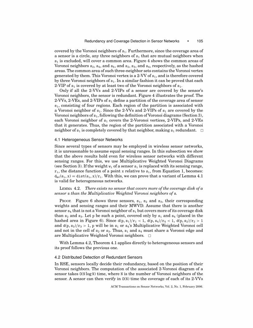
Fig. 10. Example of new sensor deployment: The gray circle, nd, represents the new sensor. (a)

The Voronoi diagram of the old sensors. The circles denote circumcircles of Delaunay triangles. (b)

The Delaunay triangulation of the old sensors.

this case, the diameter k is n/2, and two sensors that are Voronoi neighborsmay be n/2 hops away. Our experiments in Section 7.1 show that for uniformdistributions of sensors, the actual number of steps required by a sensor tocollect enough information to accurately build its Voronoi cell is much smallerthan the network’s diameter.

6.2 Deployment of New Sensors

The deployment of new sensors has the potential to change the set of redundantsensors and the coverage-boundary of the network. In both cases, this boils downto updating the local Voronoi information of the affected sensors. Figure 10illustrates an example in which a new sensor ns joins an existing network.Only sensors whose Voronoi cell is affected by the presence of the new sensorhave to be notified about the new sensor. It is well known that the circumcircleof a Delaunay triangle contains no other site (sensor). We call such a circle aDelaunay circle. Hence, only sensors that generate a Delaunay triangle whoseDelaunay circumcircle contains the new sensor, must be notified. We say thatsuch a triangle is in conflict with the new sensor, and the sensors that generatethe triangle are called notifiables. All the sensors in Figure 10 are notifiablewith regard to ns.

Before proceeding with the description of the join algorithm, we present twouseful lemmas, direct consequences of Lemmas 4.3 and 4.4 from Devillers et al.[1992].

LEMMA 6.1. Given a randomly deployed sensor network of size n, the expectednumber of sensors affected by the random deployment of a new sensor is O(log n).

LEMMA 6.2. The expected number of Voronoi neighbors of a sensor in a ran-domly deployed sensor network, is constant.

The Join Algorithm. Whenever a new sensor is deployed, it sends a beaconmessage and a sensor that receives this beacon is said to detect the new sen-sor. Thus, the new sensor can be detected by another sensor only if the radio



transmission ranges of the two sensors exceed the distance between them. Asensor that detects the presence of a new sensor needs to notify other sensorsaffected by its presence. Since more than one sensor can detect the new sen-sor, multiple, redundant notifications might be sent in the network. To avoidthis, we choose only one sensor, called introducer (S), to perform the notifica-tion. We choose S to be the sensor whose Voronoi cell contains the position ofthe newly deployed sensor. In Figure 10(a), the introducer of ns is s1. If thenew sensor is connected to the network, according to the definition of a Voronoicell (Section 3), our choice guarantees that the introducer will detect the newsensor.

The introducer initiates the notification process, and during the process,each notified sensor uses only local information to determine its behavior. Eachsensor has a list of incident Delaunay triangles, and the introducer, S, traversesits list of Delaunay triangles, identifies the ones in conflict with the new sensor,and isolates the notifiables among its Voronoi neighbors. Then, sensor S sortsits notifiables based on its Euclidean distance to them. Each sensor uses threecolors to differentiate the notifiables in its local view. Initially, all the notifiableVoronoi neighbors are white. Upon completion of the coloring algorithm, theywill be either gray or black, and the sensor, in this case S, will only contact theblack ones. A gray colored notifiable denotes a sensor that can be easier notifiedby one of the black notifiables, thus its notification should be postponed.

The coloring algorithm proceeds as follows. First, S takes its closest whitenotifiable, marks it black, and removes it from the white list. Then, it traversesthe white list in clockwise order starting from the newly removed notifiable. Ifa white notifiable, W, is part of a local Delaunay triangle that has a gray or blackvertex, G, such that dist(S, W) > dist(G, W), it marks W gray and removes it fromthe white list. Since W is closer to G than to S, it can be more easily notified by Gthan by S. If, at the end of the traversal, a notifiable has been marked gray, thetraversal is repeated, until no more white notifiables are marked gray. Then,if the white list is not empty, the closest white notifiable is again removed andmarked black and the above process is repeated. In the example from Figure 10,sensor s1 first colors sensor s2 black and in the subsequent traversal, colorssensor s3 gray. It then colors sensor s8 black, and in the first traversal colorssensor s7 gray. A second traversal colors sensor s6 gray.

On completion of the coloring phase, S sends a notification to each black no-tifiable. For such a notifiable B, the message contains the identity and positionof the new sensor, the identity of the notifier, in this case S, and the identitiesof all the gray notifiables in the local view of S, that B needs to notify. A sensorN that receives a new sensor notification, ignores the notification if it has al-ready received it from another Voronoi neighbor. Otherwise, N creates its ownwhite list of notifiable Voronoi neighbors. N removes from this list all the graysensors contained in the notification, and marks them black, since it has tonotify them. It also removes from the white list, the notifier (the sensor fromwhom it has received this notification) and marks it gray, since it should notnotify it. N then repeats the coloring phase described above, and sends to eachblack notifiable a notification with the same structure as the one that itself hasreceived.



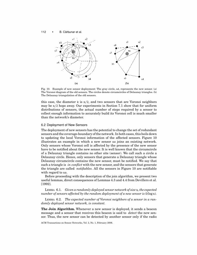
Fig. 11. Illustration of the correctness proof for the join algorithm.

Example. Figure 10 illustrates an example of the notification process. Here,ns is a newly deployed sensor. As explained above, sensor s1 sends a messageonly to sensors s2 and s8. When sensor s3 receives the notification from sensors2, it first constructs its list of notifiables, consisting of sensors s2, s4, s5, s6,and s1. It then colors sensor s2 gray, since sensor s2 is the one that sent itthe notification. It then traverses the list of notifiables. In the first traversal itcolors sensor s1 gray. We note that this is natural, since we already know thatsensor s2 is closer to sensor s1 than sensor s3. In the next traversal, sensor s3colors sensor s6 gray, since dist(s3, s6) > dist(s1, s6). The next traversal colorssensor s5 gray, and the last colors sensor s4 gray. When sensor s6 receives thenotification from sensor s7, which received it from sensor s8, it constructs itslist of notifiables, s7, s1, s3, s5. It marks sensor s7 gray and propagates the graycolor to sensors s1 and s3. It then marks sensor s5 black and notifies it. Thenotification similarly reaches sensor s4.

The local coloring and propagation of gray is meant to reduce the number ofredundant messages. Sensor s3 will not notify sensors s6, s5 and s4, since sensors8 will notify sensor s7, which in turn will notify sensor s6, and so on. Thismethod will not eliminate all redundant notifications, but by locally reducingthe distance between a notifier and a notifiable, this method has the advantageof reducing the number of actual messages that need to be sent for a notification.This is because the chance of two Voronoi neighbors of being in each other’s radiotransmission range increases when their Euclidean distance decreases.

We now present several properties of the join algorithm.

CORRECTNESS 1. Upon completion of the algorithm, all the notifiable sensorshave been notified.

PROOF. By induction on the Delaunay distance between a notifiable andthe introducer. Figure 11 illustrates the proof, where ns represents the newsensor. The basis is simple, since all notifiables at distance 1 from the introducerare clearly notified. For the induction step, we assume that all notifiables at



distance l − 1 are notified. Let s1 be a notifiable at Delaunay distance l fromthe introducer. Being a notifiable, s1 has at least a triangle in conflict with thenew sensor, ns. Since in terms of the Euclidean distance s2 and s3 are s1’s closestVoronoi neighbors to ns, the triangle �s1s2s3 is such a conflict triangle. Sensors1 is at Delaunay distance l from the introducer, si, therefore it has at leastone Voronoi neighbor at Delaunay distance l − 1 from si. Since si is the closestsensor to ns, no other Voronoi neighbor of s1 is at a smaller Delaunay distancefrom si than s2 and s3. Hence, at least one of s2 or s3 are at Delaunay distancel − 1 from si. If both are, since both are notifiable, they will both be notified. Atleast the one closer to s1 will then notify it, since both will detect the triangle�s1s2s3 to be in conflict with ns. If only one of s2 or s3 is at distance l − 1, thenthat one will notify s1.

TERMINATION 1. The algorithm will terminate—notifications will not be sentindefinitely.

PROOF. Each notifiable sensor can receive notifications only from its Voronoineighbors that are also notifiable. Only notifiable sensors receive notifications.A notifiable sensor propagates a notification only to notifiable Voronoi neigh-bors, and only when receiving a notification concerning a new sensor for thefirst time. Since the number of expected notifiables is bounded (Lemma 6.1),and each propagates a notification only once, the algorithm will terminate.

COMPLEXITY 1. The expected number of notifications for a join is O(log n),where n is the number of sensors already in the network.

PROOF. For a new sensor, the expected total number of notifiables is O(log n)(Lemma 6.1), and each notifiable receives notifications only from its Voronoineighbors that are also notifiables. Since the expected number of Voronoi neigh-bors of a sensor is constant (Lemma 6.2), the expected number of notificationsis O(log n).

We make the observation that using the construction provided in Devillerset al. [1992], a sensor affected by a join can recompute its local Voronoi digramin O(log N) expected time.

6.3 Sensor Failures

Sensor failures, like the deployment of new sensors, also require the modifica-tion of local Voronoi neighbors of affected sensors. The following lemma iden-tifies the sensors affected by a single failure, and limits the size of their set ofcandidate replacement Voronoi neighbors.

LEMMA 6.3. A single sensor failure affects the local Voronoi information be-longing only to the Voronoi neighbors of the failed sensor. Furthermore, the setof candidates for the position of new Voronoi neighbors of each affected sensorconsists solely of the Voronoi neighbors of the failed sensor.

PROOF. The direct Voronoi neighbors of the failing sensor are clearly af-fected, since one of their Voronoi neighbors disappears. To see why other sen-sors are not affected, consider the following: let f2 be a failed sensor and s6 be a



Fig. 12. Example of network where sensors f1, f2 and f3 fail simultaneously. The round arrows

show the local decisions made by intermediate sensors, and the straight arrows show the trajectory

of the DISC messages.

sensor that is not a Voronoi neighbor of f2 (Figure 12). Since f2 is not a Voronoineighbor of sensor s6, by the definition of Voronoi diagrams, there are no sen-sors in the interior of any of the Delaunay circles generated by sensor s6. Hencesensor s6 will not acquire new Voronoi neighbors. The same argument can beused to prove that the affected sensors will have to consider as candidates fornew Voronoi neighbors, only the set of affected sensors. For example, sensor f3must only consider sensors s1, s4, s5, f1, s8 to replace the position left by f2. Itneed not consider sensor s6, since s6’s Voronoi neighbors are not changed byf2’s failure.

Departure Algorithm. We now present the actions taken when one or moresensors fail, possibly simultaneously. Each sensor S periodically sends a beaconto its Voronoi neighbors. For each Voronoi neighbor, S has a timeout value thatis set whenever a beacon is received from the respective neighbor. The timeoutvalue is an upper bound on the period of the beacon plus the round-trip timefor that neighbor. If the timeout for a neighbor F expires before the respectivebeacon is received, S declares F failed and initiates a protocol to discover its newneighbors. For this, it creates a message of type DISC, containing the identityof S, a sequence number maintained by S and two lists. The sequence numberis incremented each time a failure is detected by S. The first list, called thefailed list, contains identities of sensors that are assumed to have failed, and

initially contains only F. The second one, called the affected list, is empty, buteventually collects the identities of the sensors affected by the failure of thesensors in the failed list. Sensor S sends the DISC message to its first Voronoineighbor in counterclockwise order from F.

A sensor N that receives a DISC message, is a Voronoi neighbor of F. Conse-quently, it adds its identifier to the affected list of the received DISC message.Sensor N then looks at the last item in the failed list, say G. Sensor N findsits first counterclockwise Voronoi neighbor starting from G, say H. If sensor His locally considered by sensor N to be failed, and is not already in the failedlist of the received DISC message, sensor N adds H to the failed list and repeatsthis process for the next counterclockwise Voronoi neighbor starting from H.The modified DISC message is forwarded to the first Voronoi neighbor of N, incounterclockwise order from G, that has not failed.



This procedure, similar to walking in a labyrinth with the left hand touchingthe wall, finds the smallest perimeter enclosing a cluster of simultaneouslyfailed sensors, and reaches all the sensors affected by the cluster’s failure.When the initiator S receives the DISC message that it initiated, it recomputesits Voronoi diagram and Delaunay triangulation using its local information andthe information in the affected list received with the DISC message.

Example. Figure 12 shows an example of a network in which three sensors,f1, f2, f3, fail simultaneously. Let us say that s7 detects that f1 has failed. s7creates a DISC message containing f1 in the failed list, and sends it to s8. Beforesending to f2, s8 detects that f2 has also failed, and adds f2 to the failed list. s8then forwards the DISC message to s1. Similarly, s1 adds f3 to the failed list andforwards the message to s2. When s4 receives this DISC message, it detects thatf2 and f3 are already in the failed list, so it forwards the message only to s5. Allthe intermediate sensors add their identities and positions to the affected list,so when s7 receives the DISC message that it has initiated, it is able to correctlyrecompute its Voronoi neighbors and incident Delaunay triangles.

Note. Each neighbor of a failed sensor must detect the absence of the failedsensor and generate a DISC message. The total number of messages sent istherefore on the order of the square of the number of Voronoi neighbors of thefailed sensors. The number of messages could be linear, if the ring of affectedsensors would have a leader. The leader could be chosen by each sensor, duringits lifetime, to be its closest Voronoi neighbor. This sensor, called monitor, wouldthen watch over its target’s presence. In case of failure detection, the monitorwould send two circular DISC messages, the first one collecting the informationof all the affected sensors, and the second one propagating this list to all of them.However, the simultaneous failure of a sensor and its monitor would break theprotocol, since not all the affected sensors would be notified.

We now prove several properties of the departure algorithm. Let GF = (VF, EF)be the failure graph, where VF is the set of failed sensors, and e ∈ EF is an edgebetween two sensors f1 and f2 in VF if f1 and f2 are Voronoi neighbors. For everyconnected component C in GF, let AC be the set of Voronoi neighbors of the sensorsin C, that are not themselves in C. That is, AC is the set of sensors affected bythe failure of the sensors in the connected component C. In Figure 12, f1, f2 andf3 form a connected component C of the failure graph, and AC = {s1, .., s8}. Withthese definitions, a generalization of Lemma 6.3 can be easily proved.

LEMMA 6.4. A connected component of the failure graph, C, affects only theVoronoi diagram of its Voronoi neighbors, AC. Moreover, the set of candidates forthe new Voronoi neighbors for each affected sensor in AC is contained in AC.

We prove several properties of the departure protocol.

CORRECTNESS 2. On completion of the departure algorithm, the sensors af-fected by the failures will correctly compute their new Voronoi neighbors.

PROOF. A sensor S that is affected by the failure of a sensor F, part of aconnected component C of the failure graph GF, will send a DISC message thatwill traverse all the sensors in AC. The message will collect information about



all the traversed sensors. Using Lemma 6.4, we conclude that when S receivesthe DISC message that it initiated, it will have all the information necessary forcomputing the new Voronoi neighbors.

TERMINATION 2. The departure algorithm terminates.

PROOF. The number of sensors that send DISC messages is equal to the num-ber of sensors affected by the sensor failures. Each DISC message will traverseonly sensors that are affected by failures.

COMPLEXITY 2. The total number of messages necessary to recompute theVoronoi neighbors of the sensors in the network, due to |VF | failures is O(|VF |2).

PROOF. The number of messages is upper bounded by the square of thenumber of sensors affected by the failures. The number of sensors affected by|VF | failures is O(|VF |), using Lemma 6.2.

We make the observation that using a result of Devillers et al. [1992], theexpected cost of updating the local Voronoi diagram of a sensor affected by asensor failure is O(log log N).

6.4 Routing to Voronoi Generators

We have assumed, until now, that the notification of the sensors affected byfailures or new sensor deployments is done using direct messages betweenVoronoi neighbors. In other words, we have assumed that routing is done alongthe edges of the Delaunay triangulation. However, two Voronoi neighbors maynot be within each other’s transmission range, requiring a routing protocol.LAR [Ko and Vaidya 1998], DREAM [Basagni et al. 1998], and GPSR [Karp andKung 2000] are examples of location based routing protocols that can be usedfor routing between nonadjacent Voronoi neighbors. However, in the followingtheorem, based on Muthukrishnan and Pandurangan [2003], we provide a lowerbound on the radio transmission range of sensors, that ensures that sensors thatare Voronoi neighbors are likely to be within each other’s transmission range.

THEOREM 6.1. Let n be the number of sensors randomly placed in a squareof area S, each sensor having a radio transmission range r. Then there exists

a constant c > 9 such that if r ≥√

cS log nn

, then any two sensors s1 and s2 thatare Voronoi neighbors are almost surely within each other’s transmission range(Pr(dist(s1, s2) ≤ r) → 1 when n → ∞).

PROOF. We divide the square of area S into square bins of size r/3. There are9Sr2

bins. Similar to Muthukrishnan and Pandurangan [2003], the probabilitythat a bin is empty after throwing n balls(sensors) in the initial square is

(1 − r2

9S

)n

≤ e−nr2/9S ≤ e−(c/9) log n = n−c/9. (2)

The second inequality was obtained by replacing rwith

√cS log n

n. The expected

number of empty bins is then



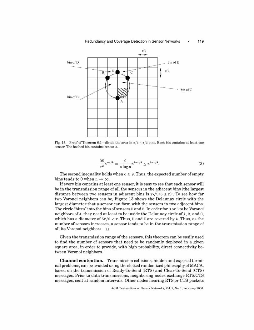
Fig. 13. Proof of Theorem 6.1—divide the area in r/3 × r/3 bins. Each bin contains at least one

sensor. The hashed bin contains sensor A.

9S

r2n−c/9 = 9

c log nn1−c/9 ≤ n1−c/9. (3)

The second inequality holds when c ≥ 9. Thus, the expected number of emptybins tends to 0 when n → ∞.

If every bin contains at least one sensor, it is easy to see that each sensor willbe in the transmission range of all the sensors in the adjacent bins (the largestdistance between two sensors in adjacent bins is r

√5/3 ≤ r) . To see how far

two Voronoi neighbors can be, Figure 13 shows the Delaunay circle with thelargest diameter that a sensor can form with the sensors in two adjacent bins.The circle “bites” into the bins of sensors D and E. In order for D or E to be Voronoineighbors of A, they need at least to be inside the Delaunay circle of A, B, and C,which has a diameter of 5r/6 < r. Thus, D and E are covered by A. Thus, as thenumber of sensors increases, a sensor tends to be in the transmission range ofall its Voronoi neighbors.

Given the transmission range of the sensors, this theorem can be easily usedto find the number of sensors that need to be randomly deployed in a givensquare area, in order to provide, with high probability, direct connectivity be-tween Voronoi neighbors.

Channel contention. Transmission collisions, hidden and exposed termi-nal problems, can be avoided using the slotted randomized philosophy of MACA,based on the transmission of Ready-To-Send (RTS) and Clear-To-Send (CTS)messages. Prior to data transmissions, neighboring nodes exchange RTS/CTSmessages, sent at random intervals. Other nodes hearing RTS or CTS packets



inhibit their transmission for the duration specified in the overheard pack-ets. Randomization is used to avoid collisions between RTS packets of sendingnodes. Data transmissions are then followed by acknowledgments, ensuringthe correct receival of data.

Delays. Sensors running our redundant sensor elimination and coverage-boundary detection algorithms base their decisions on the state of their Voronoineighbors. At various stages of the protocols, sensors need the knowledge of theredundancy or coverage-boundary status of their Voronoi neighbors or theirdecision to stay active or sleep. Message loss becomes then an important issue.

During the initial computation of Voronoi cells (see Section 6.1), messagebroadcast is the predominant operation. This makes the use of acknowledg-ments an unscalable solution for message loss problems. However, sensors canuse their knowledge of the identities of their one-hop neighbors in the followingfashion. During step i of the initial computation, each sensor s maintains a listLs of the neighbors from which it has received their step i broadcast packets,containing their network view. For this, each broadcast packet needs to containa sequence number denoting the current step of its sender. After sending its ithbroadcast packet, s starts a timer and waits for a fixed interval to receive stepi broadcast packets from all its neighbors. When the timer expires, s contactsall the neighbors that are not in Ls, in a point-to-point protocol, to exchangestep i information. The point-to-point protocol uses acknowledgments and re-transmissions to solve message loss problems. Lack of answers for a predefinednumber of retries is interpreted as a failure.

During join and departure operations, message unicast is the predominantoperation. Thus, acknowledgments and retransmissions can be similarly usedto handle message loss problems.

7. SIMULATION RESULTS

In this section, we support our analytical results with a detailed simulationstudy for quantifying the overhead and correctness of our algorithms. InSection 7.1 we evaluate the number of message exchanges needed to computethe initial Voronoi cells of sensors. In Section 7.2 we compare our coverage pre-serving redundancy elimination algorithm, RSE, with two existing algorithms,PEAS [Ye et al. 2003] and TG [Tian and Georganas 2002]. In Section 7.3 wemeasure the communication traffic generated by join and leave operations.In Section 7.4 we investigate the ability of RSE to extend the coverage andconnectivity lifetime of sensor networks.

7.1 Initial Construction of Voronoi Cells

The initial distributed computation of the Voronoi cells of sensors presentedin Section 6.1 assumes a theoretical worst case where Voronoi neighbors maybe k hops away, where k is the diameter of the network. In a worst case sce-nario, sensors have to learn of the entire network in order to accurately detecttheir Voronoi neighbors. In this subsection we measure the distance in num-ber of hops between Voronoi neighbors and the traffic load imposed on the



Fig. 14. The initial construction of the Voronoi diagram.

network by the initial computation of Voronoi cells, in realistic distributions ofsensors.

In the first experiment we use transmission ranges between 60m and200m for 700 sensors randomly distributed in a 1000 × 1000 m2 square area.Figure 14(a) shows the average number of steps and the corresponding 95%confidence interval of the heart-beat algorithm presented in Section 6.1 re-quired by a sensor to collect information about all its Voronoi neighbors. Recallthat in the lth step of the heart-beat algorithm a sensor collects informationabout sensors that are l hops away. Therefore, Figure 14(a) presents the dis-tance in number of hops between a sensor and its farthest Voronoi neighbor.The average and confidence intervals are computed over all the sensors in thenetwork. The distance in hops between farthest Voronoi neighbors quickly de-creases from almost 3 to very close to 1. For a transmission range of 90 m, asensor needs to contact sensors on average 1.2 hops away.

Figure 14(b) shows the corresponding load in terms of the number of sensorswhose identity and location information is collected by a sensor in order toaccurately compute its Voronoi diagram. After an initial decrease to 31 for atransmission range of 90 m, later the load experiences an increase to 80 fora transmission range of 200 m. This is because larger transmission rangesimply larger sensor degrees (more sensors within the communication range).However, even in this case sensors have to collect only up to 11% of the totalinformation collected when the number of hops is equal to the diameter of thenetwork.

In the second experiment we place between 200 and 1000 sensors with atransmission range of 100 m in the 106 m2 area. Figure 15(a) shows the averageand confidence interval of the distance in number of hops between a sensor andits farthest Voronoi neighbor. For higher concentrations of sensors, the distancein hops between Voronoi neighbors decreases, leading to fewer hops requiredto collect information about the Voronoi neighbors. For 450 sensors the averagenumber of hops is under 1.5. The diameter of the network is however between21 at 200 sensors and 16 at 1000 sensors. Thus, the heart-beat algorithm ofSection 6.1 can safely stop at five times fewer steps than the network diameter.

Figure 15(b) shows the corresponding average number of sensors whose in-formation is collected in the heart-beat process by a sensor. While the load



Fig. 15. The initial construction of the Voronoi diagram.

experiences an initial decrease with higher sensor densities, it later (start-ing at around 700 sensors) exhibits a mild increase. This is because highersensor densities decrease the number of steps of the heart-beat algorithm (seeFigure 15(a)) but also increase the number of sensors placed in each other’s com-munication range (sensor degree). For example, for 1000 sensors, the Voronoineighbors of a sensor are very likely 1 hop away but the average number oftransmission neighbors is between 32 and 37. However, this represents 4% ofthe information collected by the heart-beat protocol when the number of stepsemployed is the diameter of the network.

7.2 Detecting Coverage-Boundary and Redundant Sensors

In the first experiment we investigate the performance of RSE under threemetrics: the number of coverage-boundary sensors, the total number of locallydetected redundant sensors, and the total number of sensors that can be si-multaneously turned off. For all the experiments in this section, we randomlygenerate 10 different sensor network configurations, and present only the av-erage results. We measure the evolution of wireless sensor networks of 500sensors, whose sensing range is increased from 5 to 100 m. Figure 16 showsthe results. When the range is smaller than 20, all the metrics have extremevalues. However, for larger values, the number of boundary sensors decreasesdrastically to almost 10% of the total number of sensors. The number of simul-taneous turn-offs however, saturates quickly at 20%, when the sensing range isaround 50. Consequently, a relatively small sensing range is enough to detectmost of the possible simultaneous sensor turn-offs.

The following experiment compares the performance of RSE with PEAS [Yeet al. 2003] and TG [Tian and Georganas 2002] algorithms. The sensors runningRSE, PEAS, and TG have a sensing range of 50 m—we increase the total numberof sensors from 150 to 500. As specified in Tian and Georganas [2002], thesensors running TG have the ability of knowing the status (active or sleeping)of their neighbors, before making their decision. Similar to the experimentsof Ye et al. [2003], for PEAS we set the probing range of sensors to be one thirdof their sensing range. We evaluate the performance of two variants of RSE, oneused in conjunction with Luby’s [1985] MIS approximation algorithm and onewhere sensors know the state of their neighbors before deciding their own state.



Fig. 16. Evolution of the number of boundary sensors, redundant sensors and sensors that can be

turned off, for 500 sensors, when their sensing range increases from 5 to 100 m.

Fig. 17. Node scalability comparison between RSE, PEAS and TG. The number of sensors with a

sensing range of 50 m grows from 150 to 500.

Figure 17 shows the performance of RSE and TG, compared with the to-tal number of redundant sensors. As expected, the total number of redundantsensors is always larger than the number of possible simultaneous turn-offs,both for RSE and TG. In addition, both variants of RSE consistently outper-form PEAS and TG, by being able to simultaneously turn off more sensors.Note that both RSE and TG preserve the coverage of the network, however, TGmakes more conservative decisions. This is because sensors running TG decidetheir redundancy on a subset of their transmission neighbors—the sponsor-ing algorithm is only an approximation. In our experiments PEAS is able toturn off more sensors than TG, however, it does not ensure complete coverage.By using the Voronoi neighbors of sensors to decide their redundancy, RSE



Fig. 18. Plots showing the total number of messages required for the deployment of new sensors.

accurately detects all the redundant sensors. However, RSE used in conjunc-tion with Luby’s [1985] approximation algorithm, discovers a subset of the in-active sensors discovered when sensors use the state of their neighbors in theirdecision.

7.3 Network Load

We investigate the traffic generated in the network by insertions of new sen-sors and failures of existing ones. The messages generated are necessary torecompute the local Voronoi diagrams, and with it, the coverage-boundary andthe redundant sensor information. As before, we assume that all the sensorshave similar capabilities, which for these experiments consist of identical radiotransmission ranges. Note that the experiments in Section 7.2 only considerthe sensing range.

Each time a new sensor ns joins the network, new paths need to be generatedbetween the new sensor and its new Voronoi neighbors. If the new sensor is notin the transmission range of one of its Voronoi neighbors, s1, the path from nsto s1 is chosen to be the concatenation of the path between ns and the sensorclosest to it, with the path between its closest neighbor and s1, since these pathsalready exist. Even though this is not necessarily the shortest path between nsand s1, our measurements show that the communication overhead introducedby using this path is very small. Our experiments measure not only the numberof messages required to notify all the sensors affected by the new sensor, butalso the number of messages necessary for the affected sensors to contact thenew sensor.

In the first experiment, we initially place between 150 and 800 sensors ina region of size 1000 × 1000 m2. All the sensors have the same radio transmis-sion range, of 115 m. To investigate the performance of the join algorithm, foreach value of the number of sensors initially deployed, we generate 10 randomnetwork configurations, and for each configuration we insert a new sensor at150 random positions. Similarly, for sensor failures, for each of the 10 randomnetworks we randomly select 150 sensors to fail. We present only the averagevalues over 1500 measurements.

Figure 18(a) shows the results of this experiment. The average number ofmessages transmitted for each join/leave operation, decreases abruptly with the



increase in sensor density, and saturates at around 400 sensors. Even though ahigher sensor density implies a larger number of Voronoi neighbors per sensor,increasing the number of sensors that need to be notified, it also implies shorterdistances between Voronoi neighbors, thus fewer routing messages. Therefore,denser networks simplify the task of locally updating the Voronoi and coverageinformation.

In the second experiment, we place 500 sensors in the same square andincrease the transmission range from 50 to 200. Similar to the previous experi-ment, the values reported are averaged over 1500 measurements. Figure 18(b)presents the results. The average number of messages required per update de-creases quickly and saturates at a transmission range of around 120. Energy-wise, there exists a trade-off between the transmission range employed and thetotal number of messages required per update. Since the energy required pertransmission increases super-linearly with the distance, shorter transmissionranges are preferred.

7.4 Network Lifetime

In this section we investigate the ability of RSE to extend the coverage andconnectivity lifetime of sensor networks. We randomly place 500 nodes with asensing range of 50 m, in a 500 × 500 m2 network deployment area. The batteryof each node has an initial charge of 300 Joules. Following the energy modelused in Wang et al. [2003], we set the power consumption of transmit (Tx)to 1400 mW, receive to 1000 mW, idle to 830 mW, and sleep to 130 mW. Theratio between the transmission range and sensing range of nodes is 2.25. Thecoverage of the network is evaluated every 10 seconds.

Sleeping nodes periodically reactivate (see Section 4.4. In order to balancethe energy consumption over the network we investigate RSE for two globalwake up period values, of 60 and 120 seconds. When nodes are reactivated,the redundancy information is recomputed by each node. From the conflictingredundant nodes, able to leave blind points (see Section 4.3), the nodes withthe lowest battery power are elected to sleep. This policy is chosen in orderto balance the power consumption over the network, effectively extending thecoverage lifetime of the network.

Figure 19 shows the evolution of the network’s coverage in time, both forRSE and a base case where all nodes are continuously active. In the base caseall nodes run out of battery after 360 s, when the coverage of the network dropsfrom 100% to 0. However, in the case of RSE, the coverage is maintained above90% until 560s for a node reactivation period of 60 s and until 610 s for a periodof 120 s.

We evaluate the ability of RSE to extend the connectivity of a sensor networkby placing a central collection point in the top leftmost corner of the 500 × 500 m2

network deployment area. We measure connectivity as the percentage of nodesable to route to the collection point. Figure 20 compares RSE with the base casewhere nodes are continuously active. While in the base case the entire networkfails at 360 s, using RSE with a reactivation period of 60s enables sensorsto maintain a connectivity level above 90% for 660s. For a 120s re-activation



Fig. 19. Coverage lifetime of a sensor network of 500 nodes.

Fig. 20. Evolution of connectivity of a sensor network of 500 nodes.

period, a similar connectivity is maintained for 840s. In conclusion, the use ofRSE significantly extends the lifetime of the network, both in terms of coverageand connectivity.

8. CONCLUSIONS

In this article, we have studied the problem of coverage-preserving, energy-efficient redundancy elimination for extending a network’s lifetime, and therelated coverage-boundary problem. We have reduced both problems to thecomputation of Voronoi diagrams and showed how to solve them using onlylocal information. We have provided distributed and localized algorithms that



allow sensors to update their view of the solution in cases of sensor failuresand new sensor deployments. We have proved the correctness and terminationproperties of these algorithms. Our simulations show that the algorithms areefficient and scale well with the number of sensors.

ACKNOWLEDGMENTS

The authors would like to thank the anonymous reviewers for their helpfulcomments in revising the article.

REFERENCES

BASAGNI, S., CHLAMTAC, I., SYROTIUK, V. R., AND WOODWARD, B. A. 1998. A distance routing effect

algorithm for mobility (DREAM). In MobiCom ’98: Proceedings of the 4th annual ACM/IEEEinternational conference on Mobile computing and networking. ACM Press, New York, NY, USA,

76–84.

CARDEI, M. AND WU, J. 2004. Coverage in Wireless Sensor Networks. Handbook of Sensor Networks.

CRC Press.

CARLE, J. AND SIMPLOT-RYL, D. 2004. Energy efficient area monitoring for sensor networks. IEEEComput. 37, 2 (Feb.), 40–46.

CHOSET, H. 2001. Coverage for robotics—a survey of recent results. Annals of Mathematics andArtificial Intelligence 31, 113–126.

DAI, F. AND WU, J. 2003. Distributed dominant pruning in ad hoc wireless networks. In ICC ’03:Proceedings of IEEE International Conference on Communications.

DEVILLERS, O., MEISER, S., AND TEILLAUD, M. 1992. Fully dynamic Delaunay triangulation in log-

arithmic expected time per operation. Comput. Geom. Theory Appl. 2, 2, 55–80.

GUPTA, H., DAS, S. R., AND GU, Q. 2003. Connected sensor cover: self-organization of sensor net-

works for efficient query execution. In MobiHoc ’03: Proceedings of the 4th ACM InternationalSymposium on Mobile Ad Hoc Networking & Computing. ACM Press, 189–200.

HAAS, Z. May 1997. On the relaying capability of the reconfigurable wireless networks. In VTC:Proceedings of 47th IEEE Vehicular Technology Conference 2, 1148–1152.

HU, L. 1993. Topology control for multihop packet radio networks. IEEE Trans. Comm. 41, 10

(Oct.), 1474–1481.

HUANG, C.-F. AND TSENG, Y.-C. 2003. The coverage problem in a wireless sensor network. In WSNA’03: Proceedings of the 2nd ACM International Conference on Wireless Sensor Networks andApplications. ACM Press, 115–121.

JIANG, J. AND DOU, W. 2004. A coverage-preserving density control algorithm for wireless sensor

networks. In Proceedings of ADHOC-NOW.

KARP, B. AND KUNG, H. T. 2000. GPSR: Greedy perimeter stateless routing for wireless networks.

In MobiCom ’00: Proceedings of the 6th Annual International Conference on Mobile Computingand Networking. ACM Press, New York, NY, USA, 243–254.

KO, Y.-B. AND VAIDYA, N. H. 1998. Location-aided routing (LAR) in mobile ad hoc networks. In

MobiCom ’98: Proceedings of the 4th Annual ACM/IEEE International Conference on MobileComputing and Networking. ACM Press, New York, NY, USA, 66–75.

LUBY, M. 1985. A simple parallel algorithm for the maximal independent set problem. In STOC’85: Proceedings of the Seventeenth Annual ACM Symposium on Theory of Computing. ACM

Press, 1–10.

MEGUERDICHIAN, S., KOUSHANFAR, F., QU, G., AND POTKONJAK, M. 2001. Exposure in wireless ad-hoc

sensor networks. In MobiCom ’01: Proceedings of the 7th Annual International Conference onMobile Computing and Networking. ACM Press, New York, NY, USA, 139–150.

MUTHUKRISHNAN, S. AND PANDURANGAN, G. 2003. The bin-covering technique for thresholding ran-

dom geometric graph properties. Tech. Rep. 2003-39, DIMACS. November.

SHAKKOTTAI, S., SRIKANT, R., AND SHROFF, N. 2003. Unreliable sensor grids: Coverage, connectivity

and diameter. In Proceedings of IEEE INFOCOM. 2, 1073–1083.



SLIJEPCEVIC, S. AND POTKONJAK, M. 2001. Power efficient organization of wireless sensor networks.

In ICC ’01: Proceedings of IEEE International Conference on Communications.

STOJMENOVIC, I. 1999. Voronoi diagram and convex hull based geocasting and routing in wireless

networks. Tech. Rep. TR-99-11, University of Ottawa. December.

TIAN, D. AND GEORGANAS, N. D. 2002. A coverage-preserving node scheduling scheme for large

wireless sensor networks. In WSNA ’02: Proceedings of the 1st ACM International Workshop onWireless Sensor Networks and Applications. ACM Press, 32–41.

WANG, X., XING, G., ZHANG, Y., LU, C., PLESS, R., AND GILL, C. 2003. Integrated coverage and con-

nectivity configuration in wireless sensor networks. In SenSys ’03: Proceedings of the 1st Inter-national Conference on Embedded Networked Sensor Systems. ACM Press, 28–39.

YE, F., ZHONG, G., LU, S., AND ZHANG, L. 2003. PEAS: A robust energy conserving protocol for long-

lived sensor networks. In ICDCS ’03: Proceedings of the 23rd IEEE International Conference onDistributed Computing Systems.

ZHANG, H. AND HOU, J. 2004. Maintaining coverage and connectivity in large sensor networks. In

International Workshop on Theoretical and Algorithmic Aspects of Sensor, Ad hoc Wireless andPeer-to-Peer Networks.

Received December 2004; revised June 2005; accepted October 2005


Redundancy and Coverage Detection in Sensor …younis/Sensor_Networks/...Redundancy and Coverage...

Documents

Transcript of Redundancy and Coverage Detection in Sensor …younis/Sensor_Networks/...Redundancy and Coverage...