Reduced-order-based feedback control of the Kuramoto–Sivashinsky equation

Journal of Computational and Applied Mathematics 173 (2005) 1–19www.elsevier.com/locate/cam

Reduced-order-based feedback control of theKuramoto–Sivashinsky equation

C.H. Leea ;∗, H.T. Tranb

aDepartment of Mathematics, California State University, Fullerton, CA 92834-6850, USAbCenter for Research in Scienti$c Computation, North Carolina State University, Raleigh, NC 27695-8205, USA

Received 13 February 2002; received in revised form 14 January 2004

Abstract

In this paper, we consider the Kuramoto–Sivashinsky equation (KSE), which describes the long-wavemotions of a thin 5lm over a vertical plane. Solution procedures for the KSE often yield a large or in5nite-dimensional nonlinear system. We 5rst discuss two reduced-order methods, the approximate inertial manifoldand the proper orthogonal decomposition, and show that these methods can be used to obtain a reduced-ordersystem that can accurately describe the dynamics of the KSE. Moreover, from this resulting reduced-ordersystem, the feedback controller can readily be designed and synthesized. For our control techniques, we use thelinear and nonlinear quadratic regulator methods, which are the 5rst- and second-order approximated solutionsof the Hamilton–Jacobi–Bellman equation, respectively. Numerical simulations comparing the performance ofthe reduced-order-based linear and nonlinear controllers are presented.c© 2004 Published by Elsevier B.V.

Keywords: Viscous 5lm =ows; Kuramoto–Sivashinsky equation; Nonlinear feedback control; Approximate inertialmanifold; Proper orthogonal decomposition

1. Introduction

The problem of in=uencing a =uid =ow to behave in a desirable fashion has been studied bynumerous scientists over the centuries. Due to the complexity of the dynamics of =uid, the nature ofthe application, and the cost of building experimental laboratories, most studies have been conductedusing computer simulation. Even with today’s computational capabilities, numerical calculations andcontrol of many =uid dynamic problems are still considered impracticable. The main challenge liesin the continuous description of the =uid =ow, which requires solving a very large system of ordinary

∗ Corresponding author.E-mail addresses: [email protected] (C.H. Lee), [email protected] (H.T. Tran).

0377-0427/$ - see front matter c© 2004 Published by Elsevier B.V.doi:10.1016/j.cam.2004.02.021

mailto:[email protected]

mailto:[email protected]

2 C.H. Lee, H.T. Tran / Journal of Computational and Applied Mathematics 173 (2005) 1–19

diEerential equations. As a result, the controller is complicated and is of high dimension. The purposeof this study is to overcome such diFculty by taking advantage of the reduced-order techniques,called the approximate inertial manifold (AIM) and the proper orthogonal decomposition (POD)methods. Namely, we develop a technique that systematically replaces a large complicated physicalsystem by another system, which is simpler, smaller, and equivalent. The most important consequenceof this in our work is that the reduced order system is small enough to use so that one can generatea real-time on-line feedback control, whereas the system resulting from a generic discretization (e.g.,a standard 5nite diEerence or 5nite element method) would require too much time to solve, hence,rendering it inapplicable in real-time control applications.

The AIM method is based on the theory of inertial manifolds for dissipated evolutionary partialdiEerential equations and has been applied to a number of important equations in =uid dynamicsand mathematical physics [13–15,17,18,20,21,46,51]. Due to the dissipativity, all solution trajectoriesin the phase space are attracted to the global attractor, which may be complicated or even fractal.An inertial manifold for a dissipative system is, on the other hand, a 5nite dimensional Lipschitzmanifold, which is positively invariant under the solution evolution, and which attracts all boundedsets in the phase space. As a result it necessarily contains the global attractor. The solution =owrestricted to an inertial manifold is equivalent to that of a 5nite dimensional system of ordinarydiEerential equations called an inertial form. Numerical procedures to solve the inertial form areknown as the AIM methods or the nonlinear Galerkin methods, which have been employed insolving a number of important equations in =uid dynamics and mathematical physics, such as theNavier–Stokes equations [28,29,53], Burgers equation [38], reaction diEusion equations [39], theCahn–Hilliard equation [40], and the Kuramoto–Sivashinsky equation [27,52].

The POD method has received much attention in recent years as a tool to analyze complexphysical systems. In principle, the idea is to use laboratory equipment to make measurements orto use a reliable solver to compute a priori an ensemble of solutions to a physical model. Thesemeasurements or solutions are called snapshots. Applying the POD technique to these snapshotsproduces an “optimal” representation, in the sense that, it uses the least degrees of freedom torepresent the ensemble. This process is also known as the Karhunan Lo;eve procedure or principlecomponent analysis. When the POD method is applied to a physical system, it yields a system oflower dimensions, which can accurately describe the dynamics of the original full model. This is, infact, the great advantage of the POD method and, as a result, the POD technique has been widelyutilized in many applications such as modeling turbulence =ows [37,3,47,10], shear =ows [44,31],channel =ows [42,4], etc. and in pattern recognition [32]. However, the use of POD as a reduced-ordermethod for controlling is relatively new. Recently, we used POD technique to simulate and solve anoptimal control problems for growing thin 5lms in a horizontal chemical vapor deposition reactor[35] and for the BMenard convection [36]. Also, Kunisch and Volkwein [33] have used POD to controlthe Burgers equation and Banks et al. [5] have applied POD to design a feedback control for a linearthin shell model.

In this paper, we present a proof-of-concept implementation of the AIM and POD based feed-back control for the Kuramoto–Sivashinsky equation(KSE) [8,11]. KSE, which is used to describelong-wave motions of the liquid thin 5lm over a vertical plane, is given by

9�9t + �

94�9z4 +

92�9z2 + �

9�9z = 0; (1.1)

C.H. Lee, H.T. Tran / Journal of Computational and Applied Mathematics 173 (2005) 1–19 3

where z ∈ [ − �; �]; t¿ 0; �¿ 0, and are subject to the initial condition

�(z; 0) = �0(z) (1.2)

and the boundary conditions9n�9zn (−�; t) =

9n�9zn (�; t); n = 0; 1; 2; 3: (1.3)

Eq. (1.1) has also been used to describe the dynamics of laminar =ame fronts [41,48,49].In the next section, we will discuss the numerical algorithms for the solutions employing the AIM

and the POD methods. In Section 3, we will focus on the objective of our studies, that is, to controlthe dynamics of the thin 5lm =ow (1.1) using the reduced-order methods. The control techniquesthat we consider in this paper include both the linear and nonlinear quadratic regulator methods.Numerical results for the linear and nonlinear feedback control employing the AIM and the PODmethods will be analyzed and compared in the last section.

2. Reduced-order methods for the KSE

2.1. Reduced-order solution using approximate inertial manifold

The existence and uniqueness of solutions to the KSE (1.1) was 5rst shown by Nicolaenko etal. [43] with the assumption that solutions are odd and periodic. It was also shown that Eq. (1.1)is dissipative and has a 5nite-dimensional global attractor. That is, its solutions after some transienttime can be characterized by a 5nite set of basis functions. The same results were achieved laterfor the general periodic case independently in [12,23]. Stability of the KSE (1.1) has been studiedextensively over the last decade (see for instance [1,2,16,24–26,43]). The studies of the inertialmanifolds for equation (1.1) can be found in [14,17,18,30,45,52]. Also following the work of Foiasand Temam [19] one can show that for any initial value:

�0 ∈{f|� is odd; periodic and

9mf9zm ∈L2(−�; �) for m¿ 1

};

the solution belongs to a Gevrey class of regularity for all t ¿ 0. In particular, �(z; t) is analyticin the spatial variable z ∈R for all t ¿ 0. In addition, Jolly et al. [27] studied the approximateinertial manifolds for (1.1) both analytically and computationally. Kevrekidis et al. studied (1.1)numerically in [30]. Furthermore, Smyrlis and Papageorgiou [50] computed the Feigenbaum numberfor the bifurcation cascade of (1.1) as � varies.

Remark 2.1. If �0 is odd, the solution �(t) remains odd for all t. Also in the derivation of (1.1),�(t) is the integral of an odd function. Thus it is natural to restrict our solution to an odd-functionspace. We denote by H = {f∈L2

per(−�; �)|fis odd}.

Remark 2.2. The operator A := 94=9z4 along with boundary conditions (1.3) is a positive de5niteoperator. The domain of A is de5ned as

D(A) :={f∈L2

odd(−�; �) | 9nf9zn (−�) =

9nf9zn (�); for n = 0; 1; 2; 3

};


so that A−1 : L2(−�; �) → L2(−�; �) is compact (Rellich’s Lemma). Thus there exists a completeorthonormal basis {�k(z)}∞

k=1 in H , consisting of the eigenfunctions of A. In particular, we have fork = 1; : : : ;∞,

�k(z) =1√�

sin(kz) (2.1)

with the corresponding eigenvalues

�k = k4: (2.2)

Remark 2.3. We denote by b(�; �) = �9�=9z, the bilinear operator for all � and �∈H1per(−�; �)

:= {f |f; 9f9z ∈L2per(−�; �)}, then Eq. (1.1) can be rewritten in the following diEerential form

d�dt

+ �A� + A1=2� + b(�; �) = 0; (2.3)

for any �∈H1per(−�; �).

Let N be a positive integer, we de5ne a projection

PN : L2(−�; �) → Span{�k | k = 1; : : : ; N}with

QN = I − PN :

Then by letting p = PN� and q = QN�, Eq. (2.3) can be split into9p9t + �Ap + A1=2p + PNb(p + q; p + q) = 0; (2.4)

9q9t + �Aq + A1=2q + QNb(p + q; p + q) = 0; (2.5)

where � = p + q. Eqs. (2.4) and (2.5) refer to the dynamics of the slow and fast manifolds for thesolution space, respectively. Due to the existence of inertial manifold for the KSE, the dynamics ofq converges quickly to the initial manifold and remains there inde5nitely. As a result, for suFcientlylarge time and suFciently large N , 9q=9t is negligible and Eq. (2.5) yields (see [27] and referencestherein)

q = −1�A−1(QNA1=2q + QNb(p + q; p + q)): (2.6)

Solution to the in5nite-dimensional function q in (2.6) cannot be found explicitly. Instead, it can beapproximated by the function �(p), where �(·) solves the exact implicit relation

�(p) = −1�A−1(QNA1=2�(p) + QNb(p + �(p); p + �(p))): (2.7)

There are several approaches to approximating the above implicit equation. The simplest one is toassume �(p) = �0(p) = 0 which is known as the linear Galerkin method. Thus the approximatedsolution is solely p and Eqs. (2.4) and (2.5) become

9p9t + �Ap + A1=2p + PNb(p;p) = 0: (2.8)


The 5rst-order nontrivial representation of � can be approximated as

�1(p) = −1�A−1(QNA1=2�0(p) + QNb(p + �0(p); p + �0(p))) = −1

�A−1QNb(p;p): (2.9)

Following this approach, one can construct higher-order AIM solution to Eq. (2.7) using the relationof �k+1(p) = p + �k(p) for any k¿ 0. Detailed formulations and numerical convergence can befound in [27] and references therein. For our AIM solution to the KSE, we will assume �=p+�1(p)which can be found by solving the diEerential and algebraic system (2.4) and (2.9). In this case,

the approximate solution has the order of convergence of ∼ �− 3

2N+1. The numerical algorithm for

computing � is given as follows:

1. Given pi = PN (�(ti)),2. Compute QNb(pi; pi) and qi = −(1=�)A−1(QNb(pi; pi)),3. Solve for pi+1 from 9p=9t + �Ap + A1=2p + PNb(pi + qi; pi + qi) = 0,4. Repeat the process.

The AIM solution corresponding to � = 0:10, N = 10, and �0(z) = (5=√�)∑5

k=1 sin(kz) is depictedin Fig. 1. We notice the unstable behavior of �(t) as time progresses.

2.2. Reduced-order solution using proper orthogonal decomposition

In this section, we will summarize the process of 5nding the POD. Detailed description of PODas well as its mathematical properties can be found elsewhere in the literature (see, e.g., [9,35]).

Fig. 1. AIM Solution using 10 linear AIM and 10 Nonlinear AIM Modes (� = 0:10).


Let {Ui(z) : 16 i6Ns; } denote the set of Ns observations (also called snapshots). In the con-text of the KSE, these observations could be experimental measurements obtained from sensorsor numerical solutions over [ − �; �] taken at diEerent time steps. In our study, we assume that{Ui(z) : 16 i6Ns} is the set of solutions to the KSE at diEerent time steps using the AIM ap-proach. However, in principle, they could be numerical solutions to the KSE using any reliablesolver. The POD technique is designed to extract from this set of observations a coherent structure,which has the largest mean square projection on the observations. In other words, we look for afunction �POD, or the so-called POD basis element, that most resembles {Ui(z)}Ns

i=1 in the sense thatit maximizes

1Ns

Ns∑i=1

|(Ui; �POD)|2; (2.10)

subject to

(�POD; �POD) = ‖�POD‖2 = 1;

where (·; ·) and ‖ · ‖ denote the usual L2 inner product and L2-norm over [ −�; �], respectively. Wechoose a special class of trial functions for �POD to be of the form:

�POD(z) =Ns∑i=1

aiUi(z); (2.11)

where the coeFcients ai are to be determined so that �POD given by expression (2.11) provides amaximum for (2.10). To this end, let us de5ne

K(z; z′) :=1Ns

Ns∑i=1

Ui(z)Ui(z′) and R�POD :=∫ �

−�K(z; z′)�POD(z′) dz′;

where R : L2([ − �; �]) → L2([ − �; �]). Then straightforward calculations reveal that

(R�POD; �POD) =1Ns

Ns∑i=1

|(Ui ; �POD)|2:

Furthermore, it follows that

(R�POD; ) = (�POD;R ) for any �POD; ∈L2([ − �; �]):

Thus R is a nonnegative symmetric operator on L2([ − �; �]). Consequently, the problem of maxi-mizing expression (2.10) amounts to 5nding the largest eigenvalue to the eigenvalue problem

R�POD = ��POD subject to ‖�POD‖ = 1 (2.12)

or ∫ �

−�K(z; z′)�POD(z′) dz′ = ��POD with ‖�POD‖ = 1: (2.13)


Substituting expression (2.11) and the de5nition of K into Eq. (2.13), we obtainNs∑i=1

[Ns∑k=1

(1Ns

∫ �

−�Ui(z′)Uk(z′) dz′

)ak

]Ui(z) =

Ns∑i=1

�aiUi(z):

This can be rewritten as the eigenvalue problem

CV = �V;

where

Cik =1Ns

∫ �

−�Ui(z)Uk(z) dz and V =

a1

a2

...

aNs

: (2.14)

Since C is a nonnegative Hermitian matrix, it has a complete set of orthogonal eigenvectors

V1 =

a11

a12

...

a1Ns

;V2 =

a21

a22

...

a2Ns

; : : : ;VNs =

aNs1

aNs2

...

aNsNs

with the corresponding eigenvalues �1¿ �2¿ · · ·¿ �Ns ¿ 0. Thus, the solution to the optimizationproblem for (2.10) is given by

�POD1 =

Ns∑i=1

a1iUi;

where a1i are the elements of the eigenvector V1 corresponding to the largest eigenvalue �1. The

remaining POD basis elements, �i, i = 2; : : : ; Ns, are obtained by using the elements of other eigen-vectors, Vi, i = 2; : : : ; Ns.

An alternative approach [35] for 5nding the solution to maximization of (2.10) is by using theso-called Rayleigh–Ritz method for 5nding eigenvalues.

The POD basis has certain desirable properties. First, the POD modes can be shown to be or-thonormal (see, e.g., [35]). In addition, the POD coeFcients are uncorrelated [9]. Finally, POD is themost eFcient, in the sense that, for a given number of modes, N , the projection on the subspace usedfor approximation will contain the most kinetic energy possible in an average sense. More speci5-cally, suppose that we have a solution v(z; t) with v∈L2([ − �; �] × [0; T ]) and an approximation ofvN of v with respect to an arbitrary orthonormal basis i(z),

vN (z; t) =N∑i=1

ai(t) i(z);

for any arbitrary N ¿ 0. If the i(z) have been nondimensionalized, then the coeFcients ai carrythe dimension of the quantity vN . If vN (z; t) denotes the velocity and 〈·〉 denotes the time average


operator, then the average kinetic energy per unit mass is given by⟨∫ �

−�vN (z; t)vN∗(z; t) dz

⟩=

⟨N∑i=1

ai(t)a∗i (t)

⟩:

Consequently, the expression 〈aia∗i 〉 represents the average kinetic energy in the ith-mode. The

following lemma establishes the notion of optimality of the POD method.

Lemma 2.4. Let {�POD1 ; �POD

2 ; : : : ; �PODN } denote the orthonormal set of POD basis elements and

(�1; �2; : : : ; �N ) denote the corresponding set of eigenvalues. If

vN (z; t) =N∑i=1

bi(t)�PODi (z)

denotes the approximation to v with respect to this basis, then the following hold:

(a) 〈bi(t)b∗j (t)〉 = #ij�i (that is, the POD coe=cients are uncorrelated).

(b) For every N ,N∑i=1

〈bi(t)b∗i (t)〉 =

N∑i=1

�i¿N∑i=1

〈ai(t)a∗i (t)〉:

The proof of this lemma is straight forward from the optimality of the eigenvalues and can befound in [9].

2.2.1. POD solutionNumerical solutions to the KSE using the POD method described above are obtained using the

following procedure:

1. Generating snapshots. For the set of observations, we take the AIM solutions shown in Fig. 1for t dispersing equally from zero to 10 s with the increment of 0:05 s (Ns = 201).

2. Constructing the covariance matrix and its eigenvalues and eigenvectors. Let C = (Ci;j), withCi;j = 1

201 (�(ti); �(tj)). Then 5nd the eigenvalues {�i}i=201i=1 and the eigenvectors {Vi}i=201

i=1 , where�1¿ �2¿ · · ·¿ �201.

3. Obtaining the POD bases and their energy. �PODi (z)=

∑201k=1 V k

i �(z; tk) and Energy(M)=∑M

k=1 �k=∑201k=1 �k . As mentioned earlier, due to its low viscosity, our uncontrolled solution’s behaviors are

highly dynamic. The number of POD modes needed to characterize the solutions correspondsdirectly to the dynamics of the snapshots. In our case, we have � = 0:10 and M = 6, whichcorresponds to over 99:99% of energy. For higher viscosity, M is smaller.

4. Constructing POD solutions. Assume �POD(z; t) =∑M

k=1 'PODk (t)�POD(z), where 'POD

k (t) is foundthrough the linear Galerkin formulation.

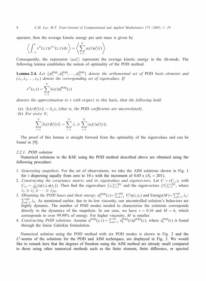
Numerical solution using the POD method with six POD modes is shown in Fig. 2 and theL2-norms of the solutions for the POD and AIM techniques, are displayed in Fig. 3. We wouldlike to remark here that the degrees of freedom using the AIM method are already small comparedto those using other numerical methods such as the 5nite element, 5nite diEerence, or spectral


Fig. 2. POD Solution using six POD Modes (� = 0:10).

0 0.5 1 1.5 2 2.5 3 3.5 4 4.5 52

4

6

8

10

12

14

16

18

20

Time (sec)

L 2 Nor

m o

f Sol

utio

n

AIMs(LIN=10 & NLR=10)POD (N=6)

Fig. 3. Relative error between the AIM solution (N = 10) and POD solution (M = 6) (� = 0:10).


methods. The number of modes needed to generate the POD solutions are also remarkably smaller.Such phenomenon is clearly due to the fact that these POD modes are used to describe a morespeci5c set of solutions, namely the snapshots. On the other hand, the 20 AIM modes can be usedto represent a larger and more general set of solutions.

3. Feedback control for the reduced-order model

As mentioned earlier, one of the applications of the KSE is to model long-wave motions ofthe liquid thin 5lm over a vertical plane. Thin liquid 5lms are ubiquitous in industrial and naturalprocesses. A simple and obvious example is the =ow of (thin) raindrop down a windowpane underthe action of gravity. Another application in the coatings industry is the wet coating of paint that isapplied to a vertical wall. The paint will =ow downward until the pain has dried; this phenomenonis called “sagging”. If the paint layer is of nonuniform thickness, with a thicker region lying abovea thin region, a relatively steep front can develop as the paint =ows downward. Often this front willdevelop undulations that lead to growing “5ngers” of paint. Such unsightly drip marks in the 5nal drycoating is undesirable for decorative purpose. Nonuniformity in the thickness of downward =owingliquid layers is also a concern in the manufacturing process of photographic 5lms where the 5lm iscreated as it passes under the falling curtain coated with thin gelatinous =uid containing chemicalssuch as light sensitive silver halide grains, dye couplers, etc. Therefore, in such applications it isdesirable to regulate the 5lm thickness at a desired constant value and as fast as possible (to speedup the process).

For small value of �, the solution to the Eq. (2.3) becomes oscillatory or unstable (see Fig. 1 or2 where � = 0:30). In this section, the optimal control problem that we formulate is to stabilize the5lm =uctuation by means of blowing or suction at the Mc points {zi}Mc

i=1 on the wall surface. Theactuators are located at {zi}Mc

i=1 ∈ [−�; �] and the proposed controllers are of the form #(z−zi)∗ui(t),where ui(t) is the control input and #(z − zi) is the Dirac delta function at zi. That is, the controlsystem is described by

9�9t + �

94�9z4 +

92�9z2 + �

9�9z = Fc(z; t); (3.1)

where

Fc(z; t) =Mc∑i=1

ui(t)#(z − zi): (3.2)

3.1. Linear and nonlinear feedback controllers

Let

�N (z; t) =N∑i=1

'i(t)�i(z)


be the approximating solution to the KSE, where {�i(z)}Ni=1 are either the Galerkin AIM or POD

bases. Then from the weak form of Eq. (3.1), we obtain

˙w(t) = Aw + N(w) + Bu; (3.3)

where

w =

'1(t)

...

'N (t)

; A = (Aij); with Aij =

∫ �

−�

(�94�i

9z4 +92 �i

9z2

)�j dz; (3.4)

N(w) =

N1(t)

...

NN (t)

with Nj(t) =

N∑i=1

N∑k=1

'i(t)'k(t)∫ �

−��i9�k

9z �j dz; (3.5)

B =

�1(z1) · · · �1(zMc)

......

�N (z1) · · · �N (zMc)

; u =

u1(t)

...

uN (t):

(3.6)

Associated with the 5nite dimensional system (3.3) is the quadratic cost functional

J (u) =∫ ∞

0

c0‖�(t)‖2

L2(−�;�) +Mc∑j=1

cj‖uj(t)‖2

dt

=∫ ∞

0

c0

N∑i=1

'i(t)2 +Mc∑j=1

cj‖uj(t)‖2

dt

=∫ ∞

0

[wTQw + uTRu

]dt; (3.7)

where ck ¿ 0 for k = 0; 1; : : : ; Mc are design parameters with Q= c0IN and R= diag{c1; : : : ; cMc}. Theoptimal control problem is to 5nd a state feedback control u∗(w) which minimizes the cost for allpossible initial conditions.

3.1.1. A linear feedback controlAssuming the nonlinear term N(w) in Eq. (3.3) is small, a suboptimal feedback control u∗ can

be obtained by using the well-known linear quadratic regulator theory. That is,

u∗(w) = − 12R

−1BT0w; (3.8)

where 0 is positive de5nite and symmetric matrix solution of the algebraic Riccati equation:

0A + AT0 − 0BR−1BTc0 + Q = 0: (3.9)


The theories for this linear quadratic regulator (LQR) problem have been well established for both the5nite and in5nite-dimensional problems (see, e.g., [6,34]). In addition, stable and robust algorithmsfor solving the Riccati equation have already been developed and are well documented in manyplaces in the literature and in textbooks.

3.1.2. A nonlinear feedback controlFor the nonlinear case, the optimal feedback control is known to be of the form

u∗(t) = − 12R

−1BTVw(w);

where the function V is the solution to the Hamilton–Jacobi–Bellman (HJB) equation

V Tw (w)(Aw + N) − 1

4VTw (w)BR−1BTVw(w) + wTQw = 0: (3.10)

The HJB equation itself is very diFcult to solve analytically for any but the simplest problems,however. Thus eEorts have been made to numerically approximate the solution of the HJB equation,or to solve a related problem producing a suboptimal control, or to use some other process in orderto obtain a usable feedback control. For a comprehensive comparison study of nonlinear feedbackcontrol methodologies we refer the interested reader to [7]. In the case where the nonlinear termN(w) is not too complex, for example, when it contains only one level of nonlinearity like thequadratic term in the KSE, the power series approximation method as proposed by Garrard andothers (see, e.g., [22]) has been shown to be very eEective [7]. In addition, it has the advantagesthat it is very easy to implement and requires less computational time as some other methods do.

In the power series method to approximate V (w), we consider the representation V (w) =∑∞

n=0 |Vn(w), where each Vn(w) = O(wn+2). Substituting the expansion into the HJB equation results in( ∞∑

n=0

(Vn)Tw

)(Aw + N(w)

)− 1

4

( ∞∑n=0

(Vn)Tw

)BR−1BT

( ∞∑n=0

(Vn)w

)+ wTQw = 0:

By separating out the powers of w we obtain the following equations:

(V0)TwAw − 1

4 (V0)TwBR

−1BT(V0)w + wTQw = 0; (3.11)

(V1)TwAw − 1

4 (V1)TwBR

−1BT(V0)w − 14 (V0)T

wBR−1BT(V1)w + (V0)T

wN(w) = 0; (3.12)

(Vn)TwAw − 1

4

n∑k=0

[(Vk)TwBR

−1BT(Vn−k)w] + (Vn−1)TwN(w) = 0; (3.13)

where n = 2; 3; 4; : : :.Eq. (3.11) can be solved with V0(w) = wT0w, where the symmetric positive de5nite matrix 0

solves the Riccati equation (3.9). This gives the standard linear control. Eqs. (3.12) and (3.13)can be solved for Vn, n = 1; 2; 3; : : :, by following the method proposed by Garrard [22]. Using the


substitution (V0)w = 20w in Eq. (3.12) we obtain

(V1)TwAw − 1

4 (V1)TwBR

−1BT(20w) − 14 (2wT0)BR−1BT(V1)w + (2wT0)N(w) = 0:

Rearranging some terms, we 5nd

wT[AT(V1)w − 0BR−1BT(V1)w + 20N(w)] = 0:

The quantity inside the brackets is zero when (V1)w = −2(AT − 0BR−1BT)−10N(w). This alongwith the (V0)w term gives a quadratic feedback control law of the form

u∗(t) = −R−1BT[0w − (AT − 0BR−1BT)−10N(w)]: (3.14)

3.2. Numerical results and comparisons

Consider � = 0:10 and the initial condition

�0(z) =5√�

5∑k=1

sin(kz);

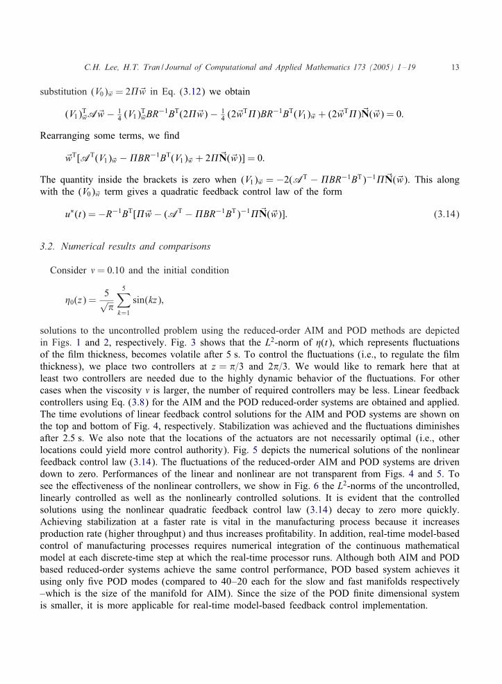
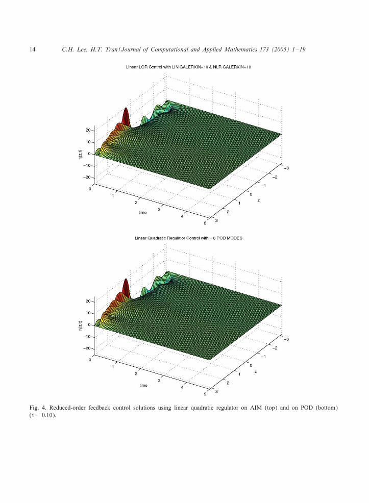
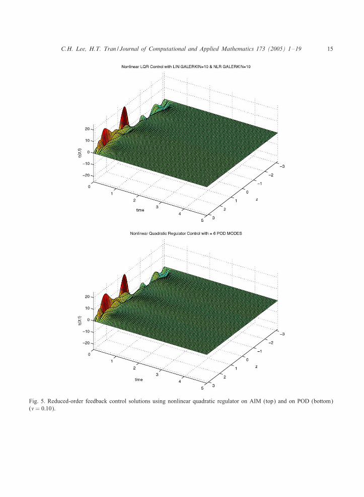
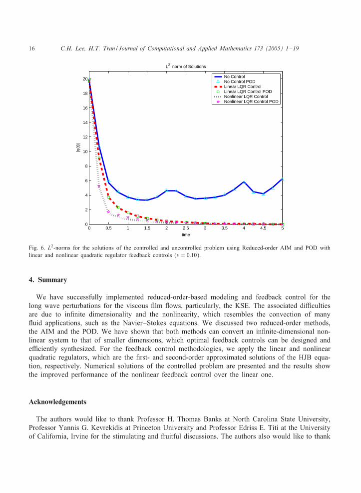
solutions to the uncontrolled problem using the reduced-order AIM and POD methods are depictedin Figs. 1 and 2, respectively. Fig. 3 shows that the L2-norm of �(t), which represents =uctuationsof the 5lm thickness, becomes volatile after 5 s. To control the =uctuations (i.e., to regulate the 5lmthickness), we place two controllers at z = �=3 and 2�=3. We would like to remark here that atleast two controllers are needed due to the highly dynamic behavior of the =uctuations. For othercases when the viscosity � is larger, the number of required controllers may be less. Linear feedbackcontrollers using Eq. (3.8) for the AIM and the POD reduced-order systems are obtained and applied.The time evolutions of linear feedback control solutions for the AIM and POD systems are shown onthe top and bottom of Fig. 4, respectively. Stabilization was achieved and the =uctuations diminishesafter 2:5 s. We also note that the locations of the actuators are not necessarily optimal (i.e., otherlocations could yield more control authority). Fig. 5 depicts the numerical solutions of the nonlinearfeedback control law (3.14). The =uctuations of the reduced-order AIM and POD systems are drivendown to zero. Performances of the linear and nonlinear are not transparent from Figs. 4 and 5. Tosee the eEectiveness of the nonlinear controllers, we show in Fig. 6 the L2-norms of the uncontrolled,linearly controlled as well as the nonlinearly controlled solutions. It is evident that the controlledsolutions using the nonlinear quadratic feedback control law (3.14) decay to zero more quickly.Achieving stabilization at a faster rate is vital in the manufacturing process because it increasesproduction rate (higher throughput) and thus increases pro5tability. In addition, real-time model-basedcontrol of manufacturing processes requires numerical integration of the continuous mathematicalmodel at each discrete-time step at which the real-time processor runs. Although both AIM and PODbased reduced-order systems achieve the same control performance, POD based system achieves itusing only 5ve POD modes (compared to 40–20 each for the slow and fast manifolds respectively–which is the size of the manifold for AIM). Since the size of the POD 5nite dimensional systemis smaller, it is more applicable for real-time model-based feedback control implementation.


Fig. 4. Reduced-order feedback control solutions using linear quadratic regulator on AIM (top) and on POD (bottom)(� = 0:10).


Fig. 5. Reduced-order feedback control solutions using nonlinear quadratic regulator on AIM (top) and on POD (bottom)(� = 0:10).


0 0.5 1 1.5 2 2.5 3 3.5 4 4.5 50

2

4

6

8

10

12

14

16

18

20

L2 norm of Solutions

time

|η(t

)|No Control No Control POD Linear LQR Control Linear LQR Control POD Nonlinear LQR Control Nonlinear LQR Control POD

Fig. 6. L2-norms for the solutions of the controlled and uncontrolled problem using Reduced-order AIM and POD withlinear and nonlinear quadratic regulator feedback controls (� = 0:10).

4. Summary

We have successfully implemented reduced-order-based modeling and feedback control for thelong wave perturbations for the viscous 5lm =ows, particularly, the KSE. The associated diFcultiesare due to in5nite dimensionality and the nonlinearity, which resembles the convection of many=uid applications, such as the Navier–Stokes equations. We discussed two reduced-order methods,the AIM and the POD. We have shown that both methods can convert an in5nite-dimensional non-linear system to that of smaller dimensions, which optimal feedback controls can be designed andeFciently synthesized. For the feedback control methodologies, we apply the linear and nonlinearquadratic regulators, which are the 5rst- and second-order approximated solutions of the HJB equa-tion, respectively. Numerical solutions of the controlled problem are presented and the results showthe improved performance of the nonlinear feedback control over the linear one.

Acknowledgements

The authors would like to thank Professor H. Thomas Banks at North Carolina State University,Professor Yannis G. Kevrekidis at Princeton University and Professor Edriss E. Titi at the Universityof California, Irvine for the stimulating and fruitful discussions. The authors also would like to thank


the Special Research Center on Optimization and Control at Karl Franzens UniversitVat Graz for theirkind hospitality during the Workshop on the Proper Orthogonal Decomposition and its Applications,when part of this work was completed. This research was partially supported by the DOD-MURIgrant F49620-95-1-0447 through the Center for Intelligent Design and Manufacturing in Electronicsand Materials and by the California State University Program for Research, Scholarship and CreativeActivity Grants at Fullerton.

References

[1] C.M. Alfaro, M.C. Depassier, A 5ve-mode bifurcation analysis of a Kuramoto–Sivashinsky equation with dispersion,Phys. Lett. A 184 (1994) 184–189.

[2] D. Armbruster, J. Guckenheimer, P. Holmes, Kuramoto–Sivashinsky dynamics on the center-unstable manifold, SIAMJ. Appl. Math. 49 (1989) 676–691.

[3] N. Aubry, P. Holmes, J.L. Lumley, E. Stone, The dynamics of coherent structures in the wall region of a turbulentboundary layer, J. Fluid Mech. 192 (1988) 115–173.

[4] K.S. Ball, L. Sirovich, L.R. Keefe, Dynamical eigenfunction decomposition of turbulent channel =ow, Internat. J.Numer. Methods Fluids 12 (1991) 585–604.

[5] H.T. Banks, R.C.H. Del Rosario, R.C. Smith, Reduced order model feedback control design: numericalimplementation in a thin shell model, Center for Research in Scienti5c Computation, North Carolina State University,Technical Report CRSC-TR98-27, 1998; IEEE Trans. AC, submitted for publication.

[6] H.T. Banks, R.C. Smith, Y. Wang, Smart Material Structures: Modeling, Estimation, and Control, Masson/Wiley,Paris/Chichester, 1996.

[7] S.C. Beeler, H.T. Tran, H.T. Banks, Feedback control methodologies for nonlinear systems, J. Optim. Theory Appl.107 (1) (2000) 1–33.

[8] D.J. Benney, Long waves in liquid 5lms, J. Math. Phys. 45 (1966) 150–155.[9] G. Berkooz, Oberservations on the proper orthogonal decomposition, in: T.B. Gatski, et al., (Eds.), Studies in

Turbulence, Springer, New York, 1992, pp. 229–247.[10] G. Berkooz, P. Holmes, J.L. Lumley, J.C. Mattingly, Low-dimensional models of coherent structures in turbulence,

Phys. Rep. 287 (1997) N4:338–384.[11] H.C. Chang, Wave evolution on a falling 5lm, Ann. Rev. Fluid Mech. 26 (1994) 103–136.[12] P. Collet, J.-P.Eckmann, H. Epstein, J. Stubbe, A global attracting set for the Kuramoto–Sivashinsky equation,

Comm. Math. Phys. 152 (1993) 203–214.[13] P. Constantin, C. Foias, Navier–Stokes Equations, University of Chicago Press, Chicago, 1982.[14] P. Constantin, C. Foias, B. Nicolaenko, R. Temam, Spectral barriers and inertial manifolds for dissipative partial

diEerential equations, J. Dyn. DiEerential Equations 1 (1989) 45–73.[15] A. Debussche, R. Temam, Inertial manifolds and their dimensions, in: S.I. Andersson, et al., (Eds.), Dynamical

Systems: Theory and Applications, World Scienti5c, Singapore, 1993.[16] C. Foias, I. Kukavica, Determining nodes for the Kuramoto–Sivashinsky equation, preprint, 1994.[17] C. Foias, B. Nicolaenko, G.R. Sell, R. Temam, Inertial manifolds for the Kuramoto–Sivashinsky equation and an

estimate of their lowest dimension, J. Math. Pures Appl. 67 (1988) 197–226.[18] C. Foias, G.R. Sell, R. Temam, Inertial manifolds for nonlinear evolutionary equations, J. DiEerential Equations 73

(1988) 309–353.[19] C. Foias, R. Temam, Gevrey class regularity for the solutions of the Navier–Stokes equations, J. Funct. Anal. 87

(1989) 359–369.[20] C. Foias, E.S. Titi, Determining nodes, 5nite diEerence schemes and inertial manifolds, Nonlinearity 4 (1991)

135–153.[21] B. Garca-Archilla, J. Novo, E.S. Titi, Postprocessing the Galerkin method: a novel approach to approximate inertial

manifolds, SIAM J. Math. Anal. 35 (N3) (1998) 941–972.[22] W.L. Garrard, D.F. Enns, S.A. Snell, Nonlinear feedback control of highly manoeuvrable aircraft, Internat. J. Control

56 (1992) N4:799–812.


[23] J. Goodman, Stability of the Kuramoto–Sivashinsky and related systems, Comm. Pure Appl. Math. 47 (1994)293–306.

[24] J.M. Hyman, B. Nicolaenko, The Kuramoto–Sivashinsky equation: a bridge between PDEs and dynamical systems,Physica D 18 (1986) 113–126.

[25] J.M. Hyman, B. Nicolaenko, Order and complexity in the Kuramoto–Sivashinsky model of weakly turbulentinterfaces, Physica D 23 (1986) 265–292.

[26] J.S. Il’yashenko, Global analysis of the phase portrait for the Kuramoto–Sivashinsky equation, J. Dyn. DiEerentialEquations 4 (1992) 585–615.

[27] M.S. Jolly, I.G. Kevrekidis, E.S. Titi, Approximate inertial manifolds for the Kuramoto–Sivashinsky equation:analysis and computations, Physica D 44 (1990) 38–60.

[28] D.A. Jones, E.S. Titi, A remark on quasi-stationary approximate inertial manifolds for the Navier–Stokes equations,SIAM J. Math. Anal. 25 (N3) (1994) 894–914.

[29] D.A. Jones, E.S. Titi, C1 approximations of inertial manifolds for dissipative nonlinear equations, J. DiEerentialEquations 127 (N1) (1996) 54–86.

[30] I.G. Kevrekidis, B. Nicolaenko, J.C. Scovel, Back in the saddle again: a computer assisted study of the Kuramoto–Sivashinsky equation, SIAM J. Appl. Math. 50 (1990) 760–790.

[31] M. Kirby, J.P. Boris, L. Sirovich, A proper orthogonal decomposition of a simulated supersonic shear layer, Internat.J. Numer. Methods Fluids 10 (1990) 411–428.

[32] M. Kirby, L. Sirovich, Application of the Karhunen–LoWeve procedure for the characterization of human faces, IEEETrans. Pattern Anal. Mach. Intell. 12 (1990) N1:103–108.

[33] K. Kunisch, S. Volkwein, Control of the Burgers equation by a reduced-order approach using proper orthogonaldecomposition, J. Optim. Theory Appl. 102 (2) (1999) 345–371.

[34] I. Lasiecka, R. Triggiani, DiEerential and Algebraic Riccati Equations with Application toBoundary/Point ControlProblems, Springer, New York, 1991.

[35] H.V. Ly, H.T. Tran, Proper orthogonal decomposition for =ow calculations and optimal control in a horizontal CVDreactor, Quart. Appl. Math. 60 (4) (2002) 631–656.

[36] H.V. Ly, H.T. Tran, Modeling and control of physical processes using proper orthogonal decomposition, Comput.Math. Appl. 33 (2001) 223–236.

[37] J.L. Lumley, The structure of inhomogeneous turbulent =ows, in: A.M. Yaglom, V.I. Tatarski (Eds.), AtmosphericTurbulence and Radio Wave Propagation, Nauka, Naurka, 1967, pp. 166–178.

[38] L.G. Margolin, D.A. Jones, An approximate inertial manifold for computing Burgers’ equation. Experimentalmathematics: computational issues in nonlinear science, Physica D 60 (N1-4) (1992) 175–184.

[39] M. Marion, Approximate inertial manifolds for the pattern formation Cahn-Hilliard equations, Math. Model Numer.Anal. 23 (1989) 463–488.

[40] M. Marion, Approximate inertial manifolds for the reaction diEusion equations in high space dimension, J. Dyn.DiEerential Equations 1 (1989) 245–267.

[41] D.M. Michelson, G.I. Sivashinsky, Nonlinear analysis of hydrodynamics instability in laminar =ames II. Numericalexperiments, Acta Astronaut. 4 (1977) 1207–1221.

[42] P. Moin, R.D. Moser, Characteristic-eddy decomposition of turbulence in a channel, J. Fluids Mech. 200 (1989) 417–509.

[43] B. Nicolaenko, B. Scheurer, R. Temam, Some global dynamical properties of the Kuramoto–Sivashinsky equation:nonlinear stability and attractors, Physica D 16 (1985) 155–183.

[44] M. Rajaee, S.K.F. Karlson, L. Sirovich, Low-dimensional description of free-shear-=ow coherent structures and theirdynamical behavior, J. Fluid Mech. 258 (1994) 1–29.

[45] J.C. Robinson, Inertial manifolds for the Kuramoto–Sivashinsky equation, Phys. Lett. A 184 (1994) 190–193.[46] G.R. Sell, Y.C. You, Inertial manifolds—the nonself-adjoint case, J. DiEerential Equations 96 (1992) 203–255.[47] L. Sirovich, Turbulence and the dynamics of coherent structures, part II: symmetries and transformations, Quart.

Appl. Math. XLV (1987) N3:573–582.[48] G.I. Sivashinsky, Nonlinear analysis of hydrodynamics instability in laminar =ames I. Derivations of basic equations,

Acta Astronaut. 4 (1977) 1177–1206.[49] G.I. Sivashinsky, On =ame propagation under conditions of stoichiometry, SIAM J. Appl. Math. 39 (1980) 67–82.


[50] Y.S. Smyrlis, D.T. Papageorgiou, Predicting chaos for in5nite dimensional dynamical systems: the Kuramoto–Sivashinsky equation, a case study, Proc. Natl. Acad. Sci. USA 88 (1991) 11129–11132.

[51] R. Temam, In5nite-Dimensional Dynamical Systems in Mechanics and Physics, Applied Mathematical Sciences, Vol.68, Springer, New York, 1988.

[52] R. Temam, X. Wang, Estimates on the lowest dimension of inertial manifolds for the Kuramoto–Sivashinsky equationin the general case, DiEerential Integral Equations 7 (1994) 1095–1108.

[53] E.S. Titi, On approximate inertial manifolds to the Navier–Stokes equations, J. Math. Anal. Appl. 149 (1990)540–557.

Reduced-order-based feedback control of the Kuramoto–Sivashinsky equation

Documents

Transcript of Reduced-order-based feedback control of the Kuramoto–Sivashinsky equation