Redes de Computadores

The Physical Layer

Manuel P. Ricardo

Faculdade de Engenharia da Universidade do Porto

1

» What service does the Physical Layer offer to Data Link Layer?

» How to encode a sequence of bits into an analogue signal?

» Why does the received signal r(t) differ from the transmitted signal s(t)?

» What is the difference between baudrate and bitrate?

» What are the advantages of the Manchester code over the NRZ code?

» What are the common digital modulations?

» What is the maximum capacity of a communications channel?

» What types of media exist and what are their main characteristics?

» What is dB, dBW, dBm, Gain, and Attenuation?

» How does the attenuation of a wireless channel vary with distance and wavelength?

2

Service Provided by the Physical Layer

Physical layer

» real communication channels used by the network

» interfaces required to transmit and receive digital data

» appears to higher layers as an unreliable virtual bit pipe

3

To Think

[Sender] [Receiver]

How to transmit the sequence of bits

110100 …

from Sender to Receiver using two wires?

4

To Think

If 1 bit is transmitted every T sec bitrate = 1/T bit/s

Why can’t we transmit infinite bitrate (bit/s) using a real cable?

5

Transmission Channel Modifies Input Signal s(t)

S H Rs(t) r(t)

h(t)

6

r(t) is the convolution of s(t) and h(t)

7

The Fourrier Transform

Using Fourrier transforms

and, in the frequency domain

Thus, r(t) depends on BH

desfSfj2

)()(

dehfHfj2

)()(

)()()( fHfSfR

fBH

f

|S(f)|

f

|H(f)|

Bs

1

BH

|R(f)|

x

=

dfefRdfefRtrftjB

B

ftjH

H

22

)()()(

8

Bandwidth-Limited Signals

(a) binary signal and its root-mean-square Fourier amplitudes

(b) – (c) Successive approximations to the original signal

9

HzT

i

Bandwidth-Limited Signals

(d) – (e) Successive approximations to the original signal.

10

Typically the receiver

» samples r(t) in order to decide about the bits transmitted

Nyquist showed that

» a signal r(t) having a bandwidth B Hz

» can be fully reconstructed

» if sampled at rate 2B sample/s

» sampling at higher rate does not provide additional information

Reconstructing de Signal the Receiver

11

Let us assume

» a square ware v(t) alternating between -5 V (bit 0) and 5 V (bit 1),

» passing through a lowpass channel BH=3kHz

If receiver samples the signal at 2BH = 6 ksample/s, it receives

» a bitrate of C=2.BH = 6 kbit/s ( 1 sample - 1 bit of information)

However,

» if M=4 levels are used to encode information– -5V(00) , -2V(01) , 2V(10), 5V(11)

» Then, the channel capacity becomes

» 2B expresses the channel baudrate in symbol/s or baud

Transmitting Information

12

skbitkMBC /12232)(log2 2

)(log2 2 MBC

To Think

Can we transmit an infinite number of bit/s in a channel of

bandwidth B=3kHz by increasing the number of levels M?

)(log2 2 MBC

13

Baseband transmission

» signal has frequencies from zero up to a maximum BH

» common for wires

Passband transmission

» signal uses band of frequencies around the frequency of the carrier fc

» common for wireless and optical channels

Baseband / Passband Transmission

14

f

|H(f)|

f2f1 fc

f

|H(f)|

1

BH

Baseband Transmission - Common Codes

NRZ-L (Non Return to Zero - Level)

» Two levels representing 0 and 1

NRZ-I (Non Return to Zero - Inverted)

» Change of level represents a 1

Manchester

» Transition in the middle of the bit

» 1: positive negative

» 0: negative positive

» Used in Ethernet (IEEE 802.3)

There are many codes …15

Clock Recovery

To decode the symbols, signals need sufficient transitions

» Otherwise long runs of 0s (or 1s) are confusing, e.g.:

Strategies:

» Manchester coding, mixes clock signal in every symbol

» 4B/5B maps 4 data bits to 5 coded bits with 1s and 0s:

Data Code Data Code Data Code Data Code

0000 11110 0100 01010 1000 10010 1100 11010

0001 01001 0101 01011 1001 10011 1101 11011

0010 10100 0110 01110 1010 10110 1110 11100

0011 10101 0111 01111 1011 10111 1111 11101

1 0 0 0 0 0 0 0 0 0 0 0 0? 0?

Bandpass Transmission

Some physical channels are bandpass

Technique used to enable s(t) to pass through h(t)

» Modulation

f

|H(f)|

f2f1

17

To Think

How to transmit bits using a continuous carrier?

18

Types of Modulations

(a) A binary signal

(b) Amplitude modulation

(c) Frequency modulation

(d) Phase modulation

Amplitude and Phase Modulations

Amplitude Modulationinformation coded in the carrier’s amplitude

Phase Modulationinformation coded in carrier’s phase

sent over a time symbol interval

tfAts ci 2cos)(

tfAts ci 2cos)(

tfsentstfts

tfsenAsentfA

tfAts

cc

cici

ci

2)(2cos)(

22coscos

2cos)(

21

20

iA

Quadrature Amplitude Modulation

Quadrature Amplitude Modulation (M-QAM)

information coded both in amplitude and phase

tfAts cii 2cos)(

21

Amplitude Modulation -

Representation in the Frequency domain

Spectrum of original signal A(t)

Spectrum of the modulated signal

( f0=fc )

Bc

Bc

22

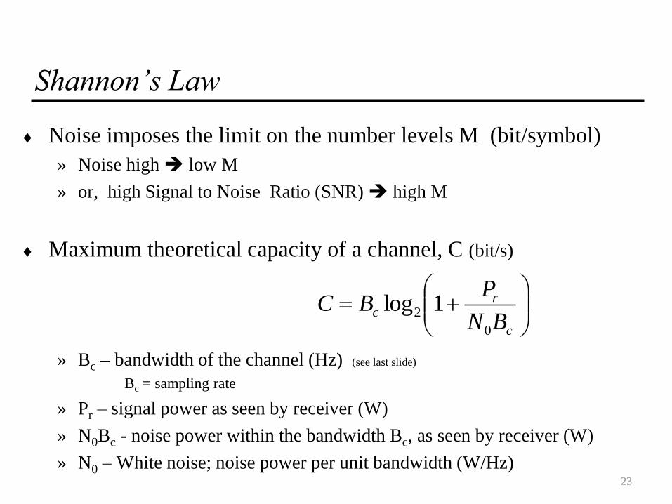
Shannon’s Law

Noise imposes the limit on the number levels M (bit/symbol)

» Noise high low M

» or, high Signal to Noise Ratio (SNR) high M

Maximum theoretical capacity of a channel, C (bit/s)

» Bc – bandwidth of the channel (Hz) (see last slide)

Bc = sampling rate

» Pr – signal power as seen by receiver (W)

» N0Bc - noise power within the bandwidth Bc, as seen by receiver (W)

» N0 – White noise; noise power per unit bandwidth (W/Hz)

c

rc

BN

PBC

0

2 1log

23

Example

If a bandpass channel has a bandwidth Bc= 100 kHz

and Signal to Noise ratio (SNR) at the receiver is

» Pr/(N0Bc)=7

» Pr/(N0Bc)=255

Power expressed in W, dBW, or dBm

» PdBW=10 log10P : P=100mW PdBW=10 log10(100*10-3)= -10 dBW

» PdBm=10 log10(P/1mW) : P=100mW PdBm=10 log10(100)= 20 dBm

skbitkC /30071log100 2

skbitkC /8002551log100 2

24

Guided Transmission

Twisted Pair

Coaxial Cable

Fiber Optics

25

Guided Transmission

Coaxial cable

Unshielded

twisted pair

Fiber optic

26

Twisted Pair

(a) Category 3 UTP.

(b) Category 5 UTP.

27

UTP Cables

From top to bottom:

Cat. 6, Cat. 5e, Cat. 5, Cat. 3

Cat 3, 16 MHz bandwidth

Cat. 5 / 5e, 100MHz

Cat. 6, 250MHz

Cat. 6a, 500MHz

Cat. 7, 600MHz

Typical attenuations 2 – 25 dB/100 m

28

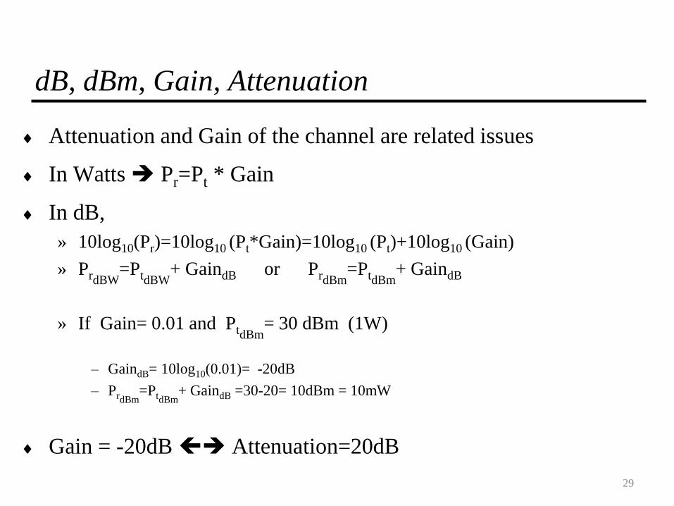
dB, dBm, Gain, Attenuation

Attenuation and Gain of the channel are related issues

In Watts Pr=Pt * Gain

In dB,

» 10log10(Pr)=10log10 (Pt*Gain)=10log10 (Pt)+10log10 (Gain)

» PrdBW=PtdBW

+ GaindB or PrdBm=PtdBm

+ GaindB

» If Gain= 0.01 and PtdBm= 30 dBm (1W)

– GaindB= 10log10(0.01)= -20dB

– PrdBm=PtdBm

+ GaindB =30-20= 10dBm = 10mW

Gain = -20dB Attenuation=20dB

29

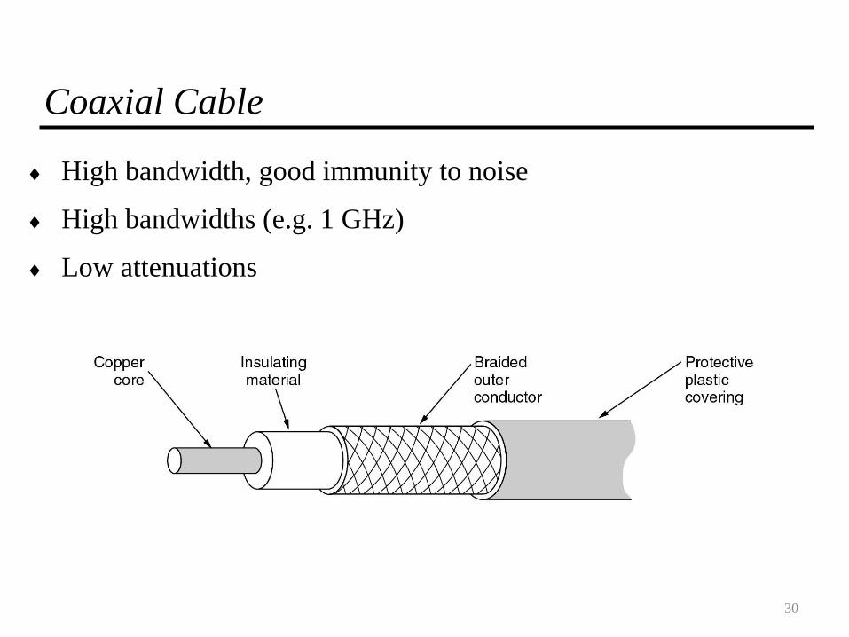
Coaxial Cable

High bandwidth, good immunity to noise

High bandwidths (e.g. 1 GHz)

Low attenuations

30

Fiber Optics

(a) Three examples of a light ray from inside a silica fiber impinging

on the air/silica boundary at different angles.

(b) Light trapped by total internal reflection.

31

Fiber Optical – Multimode vs Monomode

32

Optical Fiber

Attenuation of light through fiber in the infrared region

Bandwidths of 30 000 GHz ! Very low attenuations < 1dB/km

Data transmission: Light (1) / No light (0) NRZ

33

Wavelength(), Propagation Delay

– : wavelength

– v: velocity of the wave

– f : frequency

» Speed of ligth in free space c = 3 * 10 8 m/s

» Propagation delays ( )

– Free space (1/c):

– Coaxial cable:

– UTP:

– Optical fiber:

kms /

kms /3.3

kms /4

kms /5

kms /5speed decreases

vT vf

wavelength

d

c

t=t1

d=d1

t

T1/ f = Period

34

Wireless Transmission

The Electromagnetic Spectrum

Radio Transmission

35

The Electromagnetic Spectrum

The electromagnetic spectrum and its uses for communication

36

Radio Transmission

(a) In the VLF, LF, and MF bands, radio waves follow the

curvature of the earth.

(b) In the HF band, they bounce off the ionosphere.37

To Think

How does the attenuation of an wireless channel vary with the

distance?

38

Free Space Loss

Free space loss, ideal isotropic antenna

– Pt = signal power at transmitting antenna

– Pr = signal power at receiving antenna

– λ = carrier wavelength

– d = propagation distance between antennas

– c = speed of light 3 ×108 m/s)

Pt

Pr

=4pd( )

2

l2=

4p fd( )2

c2cf

Free Space Loss, in dB

dBdfc

fd

P

PL

r

tdB 56.147)log(20)log(20

4log20log10

Homework

1. Review slides

Important: slides do not address details (no time!). Book(s) must be read!

2. Read from Tanenbaum

» Sections 2.1, 2.2, 2.3, 2.5, 2.6, 2.8, 2.9

3. Read from Bertsekas&Gallager

» Sections 2.1, 2.2

4. Answer questions at moodle

41