RECURSIVE PARTITIONING METHODS TO …780 ever married individuals 50 years or older. ......
33
1 RECURSIVE PARTITIONING METHODS TO UNDERSTAND FACTORS ASSOCIATED WITH HUMAN LONGEVITY Gilda Garibotti 1 , Heidi Hanson 2,3 , Mike Hollingshaus 4 , Ken Smith 3,5 1 Centro Regional Universitario Bariloche, Universidad Nacional del Comahue, Argentina 2 Department of Family and Preventive Medicine, University of Utah 3 Population Sciences, Huntsman Cancer Institute, University of Utah 4 Ken C. Gardner Policy Institute, University of Utah 5 Department of Family and Consumer Studies, University of Utah
Transcript of RECURSIVE PARTITIONING METHODS TO …780 ever married individuals 50 years or older. ......

1
RECURSIVE PARTITIONING METHODS TO UNDERSTAND FACTORS ASSOCIATED WITH
HUMAN LONGEVITY
Gilda Garibotti1, Heidi Hanson2,3, Mike Hollingshaus4, Ken Smith3,5
1Centro Regional Universitario Bariloche, Universidad Nacional del Comahue, Argentina
2Department of Family and Preventive Medicine, University of Utah
3Population Sciences, Huntsman Cancer Institute, University of Utah
4Ken C. Gardner Policy Institute, University of Utah
5Department of Family and Consumer Studies, University of Utah

2
ABSTRACT
The number of forces affecting longevity are extensive and their interactions voluminous.
Biodemographers need to consider novel methodologies to identify how these numerous factors
alter the life chances of humans. We argue that recursive partitioning (RP) methods may offer a
useful approach to address this longstanding challenge. RP methods allow us to identify complex
combinations of family and individual circumstances present in early and mid-life that explain
the variability in longevity later in life. We apply this methodology to data from the Utah
Population Database (UPDB), a large biodemographic and genealogy resource. We identified
59,780 ever married individuals 50 years or older. We find that combinations of later birth
cohort, stronger family history of longevity, lower birth order, and later age at last birth are
associated with better survival. We also demonstrate the importance of ancillary methods needed
to apply RP methods to complex and large data sets.

3
INTRODUCTION
The length of life among humans is variable and the roots of this variation are complex.
Multifarious forces lead some people to outlive their expected life span, while limiting that of
others. Not only are these factors extensive but the volume of their combinations is staggeringly
large. What strategies and methodologies are available to gerontologists and biodemographers
that can aid in advancing our understanding of the many hypothesized factors affecting longevity
differentials, studied separately or in combination? In this paper, we suggest that recursive
partitioning methods have much to offer to address this challenge.
Opinions differ on the main sources of variation and the intervening mechanisms that
affect health and longevity differentials, a state of affairs that argues for the inclusion of many
indicators so that their relative influence (and their interactions) can be assessed simultaneously.
Recursive partitioning methods allow investigators to identify combinations of risk and
protective factors related to lifespan, and to quantify the relative importance of life conditions
that contribute to health and longevity differentials.
What factors and mechanisms are potentially important for inclusion? We give special
attention to circumstances that are observable and represent conditions in utero and during
infancy, childhood and mid-life (Smith et al. 2009; Yi and Vaupel 2004; Smith et al. 2014). At
the earliest, prenatal conditions such as fetal nutrition and placental characteristics are known to
influence health outcomes in adult life (Eriksson et al. 2013; Barker and Thornburg 2013;
Godfrey and Barker 2000; Doblhammer 2004; Gluckman et al. 2008). The role of malnutrition,
infections and poor health during childhood on survival and late onset disease risk has been well
documented (Hanson and Smith 2013; Huang and Elo 2009; Crimmins and Finch 2006; Case,
Fertig and Paxson 2005; Blackwell, Hayward and Crimmins 2001; Yi, Gu and Land 2007).

4
A range of family circumstances in early-life has also been studied in relation to mortality
risks later in life. Parental age at conception, sibship size, birth order, family’s socioeconomic
status, and early parental death influence offsprings’ life chances in a number of ways that have
been found to affect mortality risks of exposed children (Smith et al. 2009; Smith et al. 2014;
Huang and Elo 2009; Yi, Gu and Land 2007; Hubbard, Andrew and Rockwood 2009; Crimmins,
Kim and Seeman 2009; Kauhanen et al. 2006).
Genetic and shared familial influences on life span have received considerable attention
in biodemography and gerontology. Several investigators found that a heritable component is
present in later-life survival (Smith et al. 2009; Garibotti et al. 2006; H. Hanson 2013, Gavrilov
et al. 2002; Coumil, Legay and Schachter 2000). Smith et al. found that a summary measure of
the longevity patterns of all known blood relatives for a given individual is an important
predictor of adult mortality (Smith et al. 2009).
For early adulthood, childbearing and child rearing affect the lives and the longevity of
parents (Hurt, Ronsmans and Thomas 2006; Smith, Mineau and Bean 2002). Measures of
fertility including parity, age at first birth, age at last birth, and interbirth intervals have been
studied in relationship to longevity. There remains, however, some disagreement on the direction
of these effects (Smith et al. 2009; Yi and Vaupel 2004; Hurt, Ronsmans and Thomas 2006;
Smith et al. 2002; Penn and Smith 2007; Smith et al. 2009; Dribe 2003).
How have these important predictors of human life span been commonly studied in the
literature? The Cox proportional hazards model and its extensions are clearly the most widely
used statistical tools in studies on human aging and the method of choice for linking early and
mid-life risk factors to later health outcomes. Although these models are useful they have
limitations. In particular, even though interactions between covariates can be incorporated, they

5
have to be specified a priori, a challenge given the potentially large number of candidates
involved. Moreover, sample size often constrains the number of interactions that can be
reasonably included. As a consequence, interactions involving multiple variables are often
ignored thereby limiting hypothesis generation. However, life circumstances are intrinsically
related, with adverse events rarely arising in isolation. Individuals who lose a parent at a young
age may experience harder socioeconomic situations; premature parental death might indicate
adverse environmental conditions that also influence offspring risk of death; poor childhood
health may adversely affect health and social status in adulthood (Smith et al. 2014; Case, Fertig
and Paxson 2005).
In this study, we employ recursive partitioning (RP) methods for survival data to gain
new insights regarding circumstances present in early and mid-life that may arise in
combinations in their joint effects on mortality risk later in life. Unlike the classic application of
the Cox model, RP methods can automatically identify the main factors associated with
longevity while also detecting interactions between them without specifying them a priori. RP
methods have been extensively used in medicine, primarily for prognostic grouping of patients
based on the course of a disease (Zhang and Singer 2010). This analytical approach, though, is
relatively novel to research on aging and in studies of life course epidemiology (Kuh et al. 2003).
In gerontology, biodemography, and life course epidemiology, the challenge is to
determine the relative importance of combinations or sequences of early and mid-life conditions
that contribute to health and longevity differentials. We discuss a variable importance measure
based on random forests, an extension of the RP approach, which quantifies the relative
importance of covariates (Ishwaran et al. 2010). Identification of the most important variables
that are associated with survival differentials is necessary to expand our understanding of aging

6
but it also helps to guide development of interventions or public policies aimed at improving
long term survival and healthy lifespan (Smith et al. 2014).
The purpose of this study is to first present the logic and procedures of RP methods and
secondly to argue that these methods are valuable analytic tools for identifying complex
combinations of family and individual circumstances present in early and mid-life that explain
the variability in longevity later in life. We apply this methodology to identify factors that
characterize subjects with differing survival experience based on conditions starting early in life
and spanning through the reproductive years, and to assess the relative importance of these
factors in expanding our understanding of late life survival differentials.
DATA
The study is based on data from the Utah Population Database (UPDB). The UPDB
comprises extensive genealogical data and is linked to numerous sources of data including Utah
birth and death certificates. Nearly 9 million individuals are now represented in the database;
new data and new members are added annually as they become available. The UPDB represents
a unique and rich resource of population-based information for demographic, genetic and
epidemiological studies.
The focus of this study is on post-reproductive mortality risks. Accordingly, all survival
is based on individuals who lived to at least age 50. Individuals are sampled from sibships where
siblings are born between 1850 and 1900. This time period was selected for several reasons: (1)
family formation patterns from this period generally reflect natural fertility conditions which is
important for examining their effects prior to the advent of modern medicine and family planning
methods, (2) the first pioneers settled in Utah in 1847 and, therefore, people born after 1847 are
the first cohorts of this population with complete data in the UPDB, and (3) all individuals from

7
this era are members of extinct cohorts where death dates are observed. All analyses are sex-
specific. One male from each sibship is selected where at least one male reached age 50 and
married (if there was more than one, one was chosen at random). The comparable process is
repeated for females. Finally, to assess early and mid-life factors that may affect later life
mortality, we utilize information from three generations: the individuals themselves, their parents
and their children.
The outcome for the study is time from age 50 to death from any cause. The early and
mid-life conditions considered are birth year, family excess longevity (FEL; vide infra), parental
age at subject’s birth, subject’s sibship size, subject’s birth order, father’s socioeconomic status,
and subject’s age at parental death, and several measures of subject’s fertility (parity, age at first
birth, and age at last birth) as suggested by the historical demographic studies of the early life
effects on longevity.
Familial excess longevity (FEL) is a measure of the familial or genetic propensity of an
individual for a long or short life based on the mortality patterns of blood relatives (Kerber et al.
2001). In order to calculate FEL for an individual, excess longevity is calculated for each blood
relative aged 65 or older. Excess longevity is obtained as the difference between the observed
age at death and the expected gender and birth year-specific age at death based on a lognormal
accelerated failure time model. Then FEL is obtained as the weighted average of these excess
longevities, with weights equal to the kinship coefficients, a measure of shared genes assuming a
Mendelian mode of transmission. Only relatives who reached age 65 are considered so that the
measure is less affected by deaths from external causes that dominate younger mortality patterns.
Childhood socioeconomic status is measured based on Nam and Powers (Nam and
Powers 1983) methods using the occupation of fathers, given that mothers during this era often

8
do not have sufficient data on occupation. This index is based on the ‘usual occupation’ reported
on death certificates where higher scores are associated with higher socioeconomic status.
Subject’s age at maternal death was defined as a set of age variables. Actual age was used if the
mother died before the subject was 30. The specific value of 30 was used if the mother died after
the subject was age 30. Finally, the subject’s age at death was used if the mother outlived the
subject. A comparable approach was used for subject’s age at paternal death.
METHODS
RECURSIVE PARTITIONING (RP) METHODS
RP methods, also known as tree-based methods, were initially introduced in the context
of classification and regression (Morgan and Sonquist 1963; Breiman et al. 1984). The
development of RP methods for survival data started with work by Gordon and Olshen (1985)
and Ciampi et al. (1987). The rationale behind RP methods for survival data is to split the
covariate space to form groups of individuals which are similar according to their survival
probabilities. The first step of the RP process divides all subjects in two subgroups according to a
question posed to one of the explanatory variables. For example, “Is age at last birth 35 years or
more?” Allowable questions involve one covariate X: if X is ordered, the question has the form
“is X≥c?” for a given value c; if X is categorical the question has the form “is X in S?” where S is
any subset of categories of X. The question that defines the partition is automatically selected
among all allowable questions based on a rule that maximizes a measure of the improvement
associated to the new partition. We use the reduction in the deviance proposed by LeBlanc and
Crowley as the measure of improvement (LeBlanc and Crowley 1992). The process of splitting
the sample into two subsamples is repeated in each subgroup until the subgroups reach a
minimum size. Minimum subgroups size was set to 20, as it is usually considered. Each step

9
results in subgroups that are more homogeneous in terms of survival experience than the groups
from the previous step. The resulting model can be represented as a binary tree whose leaves or
terminal nodes correspond to the final partition of the data and yield bins of individuals who all
share a common survival profile.
This first stage of the procedure yields a large tree with many terminal nodes which
might overfit the data and fail to generalize well to the population of interest. Two additional
stages are usually performed, as we do here, after the large tree is built: pruning and
amalgamation. These stages aim at readjusting the size of the tree by combining or
amalgamating nodes with similar survival experience to form the final groups (Breiman et al.
1984; Therneau and Atkinson 2011). Summaries of the final groups are computed to interpret the
tree. When survival is the focus, Kaplan Meier curves are reported.
VARIABLE IMPORTANCE AND PARTIAL SURVIVAL FUNCTION BY RANDOM FORESTS
A random forest is an ensemble of survival trees obtained from random samples with
replacement (i.e., bootstrap samples) drawn from the original data set (Ishwaran et al. 2008).
Two estimates that we show are central to life course studies can be obtained from random
forests: variable importance measures (VIMP) and partial survival functions.
The relative importance of early and mid-life conditions that contribute to health and
longevity differentials can be quantified using VIMP. Variable importance measures based on
random forests have been proposed by several authors (Ishwaran et al. 2010; Breiman 1996;
Breiman 2001). In this article we use the VIMP offered by Ishwaran et al. (2010). The values of
this measure are associated with the depth at which a variable tends to appear in trees, with
higher values corresponding to variables that occur first in the recursive partitioning process (i.e.,
variables splitting higher in trees are more important). This measure can take both positive and

10
negative values. Large positive VIMP values indicate that the associated variable is more
predictive.
In the context of random forests, an estimate of the survival function is obtained as the
average of the Nelson-Aalen survival function estimates for each tree of the forest (Ishwaran et
al. 2008). Further understanding of the effect of covariates on survival can be gained studying
the partial survival function (i.e., the survival at a fixed point in time considered as a function of
values of a covariate). More precisely, the partial predicted survival for a covariate X at time t is
�̂�(�) =��̂��, �, ��,0�,��=1
where �̂(�, �, ��,0) denotes the random forest predicted survival at X=x and at the observed values
for observation i, xi,0, for the other variables.
STATISTICAL ANALYSES
Gender-specific multivariate Cox proportional hazards models were estimated to evaluate
the simultaneous effect of early and mid-life conditions on survival past age 50. The RP
algorithm was then used to partition the sex-specific samples into groups of individuals with
similar survival experiences after age 50, and to identify the interrelated circumstances present in
early and mid-life that characterize these groups. For each group identified by the RP method,
we report Kaplan Meier curves, and the estimated median survival, and 95% confidence interval
(CI).
The VIMP of each factor studied was calculated to evaluate its relative importance for
understanding longevity. In addition, for each of the most important life conditions encountered
we study the pattern of the random forest partial survival function estimate at the median and
third quartile sample survival times. These times were chosen to assess how values of a covariate

11
induce variations in survival with respect to the average longevity in the sample, and with respect
to one indicator of excess longevity (i.e., the third quartile). All analyses were performed with
the R 2.14.2 package. (R Core Team 2012) Recursive partitioning was done using rpart3.1-50
(Therneau 2011). Variable importance was implemented using the package
randomForestSRC1.4 (Ishwaran and Kogalur 2013).
RESULTS
In UPDB, 42,748 sibships born between 1850 and 1900 with at least one member who
reached age 50 and who was ever married were identified. Only one male and one female were
chosen from each sibship. We identified 59,780 individuals 50 years or older and ever married,
yielding the final samples comprising of 31,221 females and 28,559 males. The sample
descriptive characteristics are given in Table 1.
TABLE 1
Estimated Kaplan-Meier median survival for men and women surviving to age 50 was
74, and 78 years, respectively. Table 2 presents hazard rate ratios from single sex-specific
multivariate Cox proportional hazards models.
For both genders, mortality hazards had a negative association with birth year, and low
FEL was positively associated with mortality past age 50. Men and women in the top quartile of
the FEL distribution experienced a mortality hazard 20% lower than individuals with FEL in the
middle 50%; being in the bottom quartile of FEL was associated with a survival penalty. Men
and women whose fathers died when they were young adults (18-29 years old) had an increased
risk of mortality compared to those whose fathers died when they were 30 or older. There was
also a negative effect on female survival associated with experiencing father death during
childhood (0-4, 5-17 years) as well as experiencing mother death when they were young adults

12
(18-29 years). In general these results point to the importance of parental death when subjects
are still dependent or they are at the age where they are making the transition to adulthood (i.e.,
under age 30). Men and women who had their first child before age 20 had excess mortality
hazard rates than those starting parenthood in middle age (20-39 years); in the case of men there
was also an adverse effect regarding late initiation of parenthood (≥40 years). Late age at last
birth conferred a survival benefit for both genders.
TABLE 2
The multivariate Cox proportional hazards models assumes the same relationships for all
people in the sample and generates separate estimates for each covariate without regard to their
combined influences. However, our interest is on the diversity of combinations that might
influence later life survival. Identifying interactions, especially those involving sets of variables
is problematic within the traditional Cox proportional hazards framework, as it involves
considering all two-way and higher level interactions. Instead, we used the RP methods outlined
above that allow different predictors, different cut points, and multiple variables considered
collectively.
RECURSIVE PARTITIONING
Figure 1 shows a summary of the RP analysis for males, the tree and the estimated
survival curves for the nine terminal nodes, as well as the overall survival curve. The tree is
organized so that at each partition, individuals in the left branch have better survival past age 50
than those in the right branch. There is a six year gap in median survival among the most long-
lived group (G1) and the least long-lived one (G9).
The tree shows that the first split was based on FEL (≥54% percentile vs. <54%
percentile). This threshold partitions the sample into two groups with a three year difference in

13
median survival, 76 vs. 73 years (not shown in Figure 1). Among men with FEL that exceeds the
54% percentile, the method identified four groups with estimated median survival times ranging
from 74 to 78 years. Group G1 comprises men born during or after 1890 (top 18% percentile of
birth year), and group G4 includes men born before 1890 and whose last child was born before
they were 36 years old. The male group with the lowest median survival, G9, had individuals
with FEL<54% percentile, born before 1890, and whose last child was born before they were 36
years old.
FIGURE 1
The groups shown in Figure 1 are amalgamated (i.e., groups with similar survival
experience are combined) resulting in four groups with distinct all-cause survival past age 50.
Men in G1 and G2 have the best survival experiences and are grouped together with median
survival age of 77 years (95% CI: 76, 77). G3 has a distinct survival experience and was not
combined with any other group. A group with intermediate longevity is formed combining G4,
G5, G6 and G7, resulting in a median survival of 74 years (95% CI: 73, 74). The two groups
with the worse survival, G8 and G9, are joined into a group with median survival of 72 years
(95% CI: 71, 72). The Kaplan-Meier estimates of the four amalgamated groups are shown in
Figure 2.
FIGURE 2
Although twelve early and mid-life conditions were included in the recursive partitioning
analysis, only four conditions appeared in the final tree presented in Figure 1: FEL, age at last
birth, birth year, and birth order. Larger values of the first three factors were associated with a
more favorable outcome, while for birth order having been born first or second represented a
survival advantage.

14
The summary of the RP analysis for females is presented in Figure 3. Female median
survival ranged from 74 years (G9) to 83 years (G1). FEL, birth year, age at first birth and birth
order are the early and mid-life conditions that determined these groupings. Unlike in the male
case, being the first child represented a liability regarding later life survival. Among women with
the worst outcome, being teenage mothers (age at first birth<20 years) played an important role
in later life survival; 74 years median survival for women starting maternity as teenagers
compared to 76 years for those starting maternity later in life.
FIGURE 3
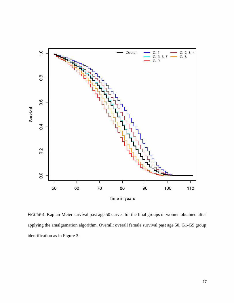
The amalgamation process merged the groups with intermediate survival experience in
two groups, one joining G2, G3 and G4 and another one combining G5, G6 and G7 (Figure 4).
The median survival was 80 years (95% CI: 80, 81) for the former and 78 years (95% CI: 78, 78)
for the latter. G1, G8 and G9 have distinct survival experiences and are not combined with other
groups.
FIGURE 4
VARIABLE IMPORTANCE AND PARTIAL SURVIVAL FUNCTION BY RANDOM FORESTS
Figure 5 provides information on the relative contribution of each early and mid-life
condition in predicting later life survival. Familial excess longevity (FEL) is clearly the strongest
predictor for males and females. The next most important predictor for males is age at last birth,
while for females both birth year and age at first birth contribute considerably to predicting later
life survival.
FIGURE 5
The random forest estimate of the partial survival function of FEL for males assessed at
the median survival time (i.e., the survival at age 74 considered as a function of FEL) increases

15
sharply for those at the absolute bottom to those at the 10% of FEL. That is, men with the
minimum value of FEL have an estimated 35% survival at age 74 while those at the 10%
percentile of FEL have a 45% estimated chance of survival at the same age (i.e., the initial abrupt
rise in the curve). The partial survival function then shows a plateau for men between the 10%
and the 40% percentile of FEL and above that it continues to increase at an approximately
constant rate (Figure S1a). A similar pattern was found for survival at age 82 (third quartile of
survival age); survival past age 82 rises from 15% for men with the minimum value of FEL to
above 30% for people at the 60th percentile of FEL (Figure S1b). The estimated survival at 74
and 82 years increases steadily with increasing ages at last birth (Figures S2a-b). At age 74, men
whose last birth was at age 30 have a below average predicted survival of 43%, compared to a
predicted survival above 52% for those whose last child was born after age 40.
For women, the estimated partial survival of FEL at the median follow up time, 78 years,
increases sharply for people in the bottom 10% of FEL, rising from about 28% for people with
the lowest values of FEL to 40% for people in the top 10% percentile of FEL. After that, the
predicted survival stabilizes up to the 25% percentile of FEL and then it continues to show an
upward trend (Figure S3a). Survival at 85 years (third quartile of follow up time) also increases
as FEL increases, from approximately 13% for women with the lowest values of FEL to above
30% for people in the top 20% of FEL (Figure S3b). Survival both at age 78 and 85 increases
steadily with birth year (Figures S4a-b). Regarding age at first birth, survival at age 78 and 85
increases rapidly from age 15 to age 22, then it shows a decreasing trend (Figure S5a-b).
We should emphasize that the partial survival function is derived from survival trees.
Accordingly, all the curves shown in Figures S1-S5 account for all the interactions with the other
variables.

16
DISCUSSION
This study examined a diverse and well-documented set of early and mid-life conditions
and, using a novel approach via RP methods, identified combinations among these predictors
that relate to longevity differentials past age 50. In addition, using VIMP measures we assessed
the relative contribution of early and mid-life conditions in their effects on longevity
discrepancies.
Beyond the well demonstrated main effects of FEL on later life survival (Smith et al.
2009; Smith et al. 2014), we identified interactions of FEL with other life circumstances. For
males in the top half of the FEL distribution (FEL≥54%), interactions with birth year, and age at
last birth were encountered, resulting in median over-all survival probabilities ranging from an
exceptionally high of 78 years to an average median of 74 years. Among women in the top 45%
of FEL, mortality risks differed depending on birth year, and birth order; RP identified a group of
women with an exceptionally high median all-cause survival past age 50 of 83 years (G1).
Interestingly, women with FEL in the bottom 45%, born in or after 1884 (G7) have a similar
mortality risk to groups of female with FEL in the top 45% percentile born before 1884 (G5 and
G6), suggesting an interesting interplay between the overall effects of history (as reflected by
birth year) separate from family history. It is worth noting that while the Cox regression analyses
also showed that FEL was significantly associated with survival, the RP analysis allows for a
more precise identification of the subpopulations whose longevity is enhanced or penalized.
A better understanding of factors affecting human longevity requires analytical tools that
take into account the interrelation between events occurring throughout life. This study has
shown how the RP method represents a valuable methodology to uncover interactions between
life circumstances in relation to mortality risks in later life. Figures 1 and 3 allow us to visualize

17
the complicated ways in which early and mid-life conditions co-occur to produce longevity
patterns in males and females. Within the Cox regression methodology, only interactions
specified a priori in the model by the analyst can be evaluated, the RP approach builds a model
in a more flexible way. Another advantage of the RP method over the traditional Cox approach is
that it automatically categorizes numerical predictors guaranteeing that the survival pattern for a
final group of individuals is homogeneous within that group; while in the traditional Cox
approach the categorization has to be decided a priori by the investigator with no guarantee of
homogeneity within the group. Also, the recursive nature of the RP method allows the
identification of prognostic factors that exert their influence in subsets of subjects rather than
across all subjects as with the Cox regression model. A limitation of the approach is due to the
known sensitivity of trees to the characteristics of the sample. Also, control parameters provided
to the algorithm such as the minimum terminal node size are arbitrarily chosen and may
influence the final description. The R program used for building the tree, rpart, produces a
number of trees that are within one standard deviation from the optimal tree. The researcher is
tasked to choose among these trees based on the context of the problem (Breiman et al. 1984).
The variable importance measure, based on an ensemble of survival trees, is a useful
technique for answering questions regarding early and mid-life conditions that are most
important for understanding variation in mortality risk later in life. For men, the main factors
associated with later life survival were FEL, and age at last birth. For women, the strongest
predictors were FEL, birth year, and age at first birth.
As in our previous work, FEL was found to be an important predictor of mortality risk
after the reproductive years both for males and females (Smith et al. 2009; Smith et al. 2014;
Garibotti et al. 2006). Higher values of FEL confer a protection on survival after the reproductive

18
years; the average probability of survival at the sample median age at death, 74 years for males
and 78 years for females increases continuously as FEL increases (Figures S1, and S3).
Association between fertility patterns and post-reproductive longevity had been reported (Smith,
Mineau and Bean 2002).
This study contributes to understanding the complexity of the interrelations between early
and mid-life conditions that account for survival decades later. The study also shows that the
recursive partitioning, and random forest methodologies are valuable tools to study determinants
of longevity.
AKNOWLEDGMENTS
This work was supported by the National Institutes of Health – National Institute of
Aging [Grant Numbers 1R21AG036938-01, 2R01 AG022095] and the Universidad Nacional del
Comahue, grant from the Research Secretary B188. The authors wish to thank the Huntsman
Cancer Foundation for database support provided to the Pedigree and Population Resource of the
HCI, University of Utah. Partial support for all datasets within the UPDB was provided by the
HCI Cancer Center Support Grant, P30 CA42014 from National Cancer Institute. We also thank
Alison Fraser and Diana Lane Reed for valuable assistance in managing the data.

19
REFERENCES
Barker, DJ, and KL Thornburg. 2013. Placental programming of chonic diseases, cancer and lifespan: a review. Placenta 34 (10): 841-5.
Blackwell, DL, MD Hayward, and EM Crimmins. 2001. Does childhood health affect chronic morbidity in later life? Soc Sci Med 52 (8): 1269-84.
Breiman, L. 1996. Bagging predictors. Machine Learning 24: 123-140.
Breiman, L. 2001. Random forests. Machine Learning 45: 5-32.
Breiman, L, JH Friedman, RA Olsehn, and CJ Stone. 1984. Classification and regression trees. Wadsworth International Group.
Case, A, A Fertig, and C Paxson. 2005. The lasting impact of childhood health and circumstances. J Health Econ 24 (2): 365-89.
Ciampi, A, CH Chang, S Hogg, and S McKinney. 1987. Recursive partitioning: a versatile method for exploratory data analysis in biostatistics. Edited by Umphrey GJ Mc Neil IB. Joshi Feistschrift, Biostatistics. 23-50.
Coumil, A, JM Legay, and F Schachter. 2000. Evidence of sex-linked effects on the inheritance of human longevity: a population-based study in the Valserine valley (French Jura), 18-20th centuries. Proc Biol Sci 267: 1021-25.
Crimmins, EM, and CE Finch. 2006. Infection, inflamation, height and longevity. Proc Natl Acad Sci 103: 498-503.
Crimmins, EM, JK Kim, and TE Seeman. 2009. Poverty and biological risk: the earlier "aging" of the poor. J Gerontol A Biol Sci Med Sci 64 (2): 286-92.
Doblhammer, G. 2004. The late life legacy of very early life. Heilderberg: Springer-Verlag.
Dribe, M. 2003. Childbearing history and mortality in later life. Lund Papers in Economic History 86.
Eriksson, JG, E Kajantie, DI Phillips, C Osmond, KL Thornburg, and DJ Barker. 2013. The developmental origins of chronic rheumatic heart disease. Am J Hum Biol 25 (5): 655-8.
Garibotti, G, KR Smith, RA Kerber, and KM Boucher. 2006. Longevity and correlated frailty in multigenerational families. J Gerontol A Biol Sci Med Sci 61 (12): 1253-61.
Gavrilov, LA, NS Gavrilovna, SJ Olshansky, and BA Carnes.2002. Genealogical data and the biodemography of human longevity. Soc Biol 49: 160-73.

20
Gluckman, DP, MA Hanson, C Cooper, and KL Thornburg. 2008. Effect of in utero and early-life conditions on adult health disease. N Engl J Med 359 (1): 61-73.
Godfrey, KM, and DJ Barker. 2000. Fetal nutrition and adult disease. Am J Clin Nutr 71 (5): 1344S-52S.
Gordon, I, and R Olshen. 1985. Tree-structured survival analysis. Cancer Treat Rep 69: 1065-9.
Hanson, H, and K Smith. 2013. Early origins of longevity: prenatal exposures to food shortage among early Utah pioneers. Journal of Developmental Origins of Health and Disease 4 (2): 170-81.
Hanson, HA. 2013. Understanding the determinants of aging and longevity: the influence of the social environment, biology, and heritability throughout the life course. Thesis, Sociology, University of Utah.
Huang, C, and IT Elo. 2009. Mortality of the oldets old Chinese: the role of early-life nutritional status, socio-economic conditions, and sibling sex-composition. Popul Stud 63 (1): 7-20.
Hubbard, RE, MK Andrew, and K Rockwood. 2009. Effect of parental age at birth on the accumulation of deficit, frailty and survival in older adults. Age Ageing 38 (4): 380-5.
Hurt, LS, C Ronsmans, and SL Thomas. 2006. The effect of number of birth on women's mortality: systematic review of the evidence for women who have completed their childbearing. Popul Stud 60 (1): 55-71.
Ishwaran, H, and UB Kogalur. 2013. R package randomForestSRC: random forests for survival, regression and classification.
Ishwaran, H, UB Kogalur, EH Blackstone, and MS Lauer. 2008. Random survival forests. Annals of Applied Statistics 2 (3): 841-60.
Ishwaran, H, UB Kogalur, EZ Gorodeski, AJ Minn, and MS Lauer. 2010. High dimensional variable selection for survival data. J Amer Statist Assoc 105: 205-17.
Kauhanen, L, HM Lakka, JW Lynch, and J Kauhanen. 2006. Social disadvantages in childhood and risk of all-cause death and cardiovascular disease in later life: a comparison of historical and retrospective childhood information. Int J Epidemiol 35 (4): 962-8.
Kerber, RA, E O'Brien, KR Smith, and RM Cawthon. 2001. Familial excess longevity in Utah genealogies. J Gerontol Biol Sci 6A: B130-B139.
Kuh, D, Y Ben-Shlomo, J Lynch, J Hallqvist, and C Power. 2003. Life course epidemiology. J Epidemiol Community Health 57 (10): 778.

21
LeBlanc, M, and J Crowley. 1992. Relative risk trees for censored survival data. Biometrics 48: 411-25.
Morgan, J, and J Sonquist. 1963. Problems in the analysis of survey data and a proposal. J Am Stat Assoc 58: 415-34.
Nam, CB, and M Powers. 1983. The socioeconomic approach to status measurements. Houston: Cap and Grown Press.
Penn, DJ, and KR Smith. 2007. Differential fitness costs of reproduction between the sexes. Proc Natl Acad Sci USA 104 (2): 553-8.
R Core Team. 2012. R: a language and environment for statistical computig. R foundation for statistical computing, Vienna, Austria.
Smith, KR, A Gagnon, RM Cawthon, GP Mineau, R Mazan, and B Desjardins. 2009. Family aggregarion of survival and late female reproduction. J Gerontol A Biol Sci Med Sci 64 (7): 740-4.
Smith, KR, GP Mineau, and LL Bean. 2002. Fertility and post-reproductive longevity. Soc Biol 49 (3-4): 185-205.
Smith, KR, GP Mineau, G Garibotti, and R Kerber. 2009. Effects of childhood and middle-adulthood family conditions on later-life mortality: evidence from the Utah Population Database, 1850-2002. Soc Sci Med 68 (9): 1649-58.
Smith, KR, HA Hanson, MC Norton, MS Hollingshaus, and GP Mineau. 2014. Survival of offsprings who experience early parental death: Early life conditions and later-life mortality. Soc Sci Med 119: 180-90.
Therneau, TM, and B Atkinson. 2011. R package rpart: Recursive Partitioning.
Therneau, TM, and EJ Atkinson. 2011. An introduction to recursive partitioning using the RPART routines. Mayo Foundation.
Yi, Z, and JW Vaupel. 2004. Association of late childbearing with healthy longevity among the oldest-old in China. Popul Stud (Camb) 58 (1): 37-53.
Yi, Z, D Gu, and KC Land. 2007. The association of childhood socioeconomic conditions with healthy longevity at the oldest-old ages in China. Demography 44 (3): 497-518.
Zhang, H, and BH Singer. 2010. Recursive partitioning and applications. 2nd. Springer.

22
TABLE 1. Descriptive statistics of early and mid-life conditions by gender.
Variable
Males Females
Mean Standard
deviation Mean
Standard
deviation
Age at death 73.71 11.03 76.65 11.55
Birth year 1876.63 12.50 1876.16 12.33
Father<20 yrs old at subject birth 0.004 0.060 0.003 0.058
Father≥50 yrs old at subject birth 0.094 0.292 0.093 0.290
Mother<20 yrs old at subject birth 0.061 0.239 0.065 0.246
Mother≥40 yrs old at subject birth 0.085 0.278 0.084 0.278
Sibship size 7.29 3.39 7.34 3.37
Birth order 3.22 2.75 3.35 2.77
Father’s Nam Power 43.20 15.01 43.14 15.00
Subject 0-4 yrs old at father death 0.034 0.181 0.036 0.186
Subject 5-17 yrs old at father death 0.120 0.325 0.122 0.327
Subject 18-29 yrs old at father death 0.185 0.389 0.187 0.390
Subject 0-4 yrs old at mother death 0.046 0.209 0.046 0.209
Subject 5-17 yrs old at mother death 0.106 0.308 0.108 0.311
Subject 18-29 yrs old at mother death 0.117 0.322 0.114 0.318
Parity 5.84 3.38 6.12 3.35
Age at first birth<20 yrs old 0.016 0.126 0.194 0.395
Age at first birth≥40 yrs old 0.050 0.219 0.009 0.094
Age at last birth 35-44 yrs old 0.463 0.499 0.633 0.482
Age at last birth≥45 yrs old 0.336 0.472 0.069 0.253

23
TABLE 2. Hazard rate ratios from multivariate Cox proportional hazards models.
Variable Males Females
Hazard rate P Hazard rate P
Birth year 0.993 <0.001 0.989 <0.001
Top 25th percentile of FEL 0.802 <0.001 0.805 <0.001
Bottom 25th percentile of FEL 1.280 <0.001 1.248 <0.001
Father<20 yrs old at subject birth 1.107 0.439 0.895 0.417
Father≥50 yrs old at subject birth 0.988 0.678 0.956 0.115
Mother<20 yrs old at subject birth 1.022 0.529 1.065 0.059
Mother≥40 at subject birth 0.978 0.470 0.990 0.751
Sibship size 1.006 0.068 1.004 0.183
Birth order 1.000 0.978 0.995 0.250
Father’s Nam Power 1.000 0.605 0.999 0.075
Subject 0-4 yrs old at father death 1.001 0.975 1.096 0.032
Subject 5-17 yrs old at father death 1.014 0.577 1.067 0.010
Subject 18-29 yrs old at father death 1.062 0.004 1.059 0.007
Subject 0-4 yrs old at mother death 1.041 0.293 1.014 0.706
Subject 5-17 yrs old at mother death 1.015 0.551 0.963 0.129
Subject 18-29 yrs old at mother death 1.016 0.505 1.074 0.004
Parity 0.999 0.822 1.004 0.229
Age at first birth<20 yrs old 1.158 0.016 1.104 <0.001
Age at first birth≥40 yrs old 1.109 0.016 1.040 0.654
Age at last birth 35-44 yrs old 0.898 <0.001 0.975 0.229
Age at last birth≥45 yrs old 0.827 <0.001 0.877 0.001

24
FIGURE 1. Recursive partitioning (RP) analysis for male sample. a) RP tree: In each terminal node the following information is given: group identification (G1-G9), n: sample size, p50: Kaplan-Meier median survival estimate, and 95% confidence intervals. alb: age at last birth, brthord: birth order, byr: birth year, FEL: familial excess longevity (given as percentile with respect total data set), b) Kaplan-Meier survival past age 50 curves for groups defined by terminal nodes of RP algorithm (a).

25
FIGURE 2. Kaplan-Meier survival past age 50 curves for the final groups of men obtained after
applying the amalgamation algorithm. Overall: overall male survival past age 50, G1-G9 group
identification as in Figure 1 a.

26
FIGURE 3. Recursive partitioning tree for female sample. In each terminal node the following
information is given: group identification (G1-G9), n: sample size, p50: Kaplan-Meier median
survival estimate, and 95% confidence intervals. afb: age at first birth, brthord: birth order, byr:
birth year, FEL: family excess longevity (given as percentile with respect to total data set).
27
FIGURE 4. Kaplan-Meier survival past age 50 curves for the final groups of women obtained after
applying the amalgamation algorithm. Overall: overall female survival past age 50, G1-G9 group
identification as in Figure 3.

28
FIGURE 5. Variable importance by random forest results of early and mid-life conditions in
predicting survival past age 50. a. Male, b. Female.
byr: birth year, FEL: family excess longevity, ma.age.bth: maternal age at subject birth,
pa.age.bth: paternal age at subject birth, sibsize: sibship size, brthord: birth order, SES: father’s
socioeconomic status, age.ma.dth: age at maternal death, age.pa.dth: age at paternal death, ceb:
parity, afb: age at first birth, alb: age at last birth.

29
APENDIX A. Supplementary figures
FIGURE S1. Male random forest estimated partial survival functions for FEL. a. at 74 years of
age, b. at 82 years of age.

30
FIGURE S2. Male random forest estimated partial survival functions for age at maternal death. a.
at 74 years of age, b. at 82 years of age.

31
FIGURE S3. Female random forest estimated partial survival functions for FEL. a. at 78 years of
age, b. at 85 years of age.

32
FIGURE S4. Female random forest estimated partial survival functions for birth year. a. at 78
years of age, b. at 85 years of age.

33
FIGURE S5. Female random forest estimated partial survival functions for age at maternal death.
a. at 78 years of age, b. at 85 years of age.