Recurrent Neural Networks for Text Classi cation · Recurrent Neural Networks for Text Classi...

Recurrent Neural Networks for Text Classification

Lecture Notes on Deep Learning

Avi Kak and Charles Bouman

Purdue University

Thursday 21st May, 2020 09:47

Purdue University 1

Preamble

In a neural network with feedback, each output creates a context for the nextinput.

This can be useful in data processing applications that produce variable-lengthinput data for a neural network. Such applications include text processing, naturallanguage translation, speech understanding, etc.

Focusing on text processing, the meaning of a word in a sentence is oftenambiguous if the word is considered in isolation from what came before it. Ingeneral, as you are reading text, in order to understand what a word or a phrase issaying, you have to bring to bear on it what you have already looked at. That is,as you read text, you understand each word and each phrase in the contextcreated by what you have read so far.

As you will see in this lecture, such contexts can be created by a neural networkwith feedback and the estimated contexts used to interpret each new input.

Purdue University 2

Preamble (contd.)

Neural networks with feedback are more commonly known as Recurrent NeuralNetworks. The torch.nn module now also comes with a class namedtorch.nn.RNN that saves you the bother of having to be explicit about thefeedback required by such networks. Here is the documentation page for thisclass:

https://pytorch.org/docs/stable/nn.html#recurrent-layers

The goal of this lecture is to:

Introduce you to recurrent neural networks with the help of a couple ofexamples;

Point to the fact that, in general, the vanishing gradient problem is evenmore acute for recurrent neural networks on account of the long chains ofdependencies created by the feedback; and

To talk about the gating mechanisms that are used to get around thischallenge.

In particular, I’ll focus on the problem of what is known as the SentimentAnalytics when highlighting the challenges of using RNNs for thisapplication.

Purdue University 3

https://pytorch.org/docs/stable/nn.html#recurrent-layers

Preamble (contd.)

Version 1.1.4 of DLStudio includes the code shown in this lecture and also theSentiment Analysis dataset I have constructed from the publicly availableuser-feedback data provided by Amazon for the year 2007.

The over 1 GB compressed archive made available by Amazon contains userfeedback on 25 product categories. Each product category contains a file with thepositive feedback comments and a file with the negative feedback comments.These have been marked so by human annotators. These are in addition to a lotof other information made available by Amazon. I have separated out just adesignated number of the positive and the negative comments for training RNNs.

Since the ultimate motivation for a novel engineering solution is the problemitself, I’ll start this lecture by first talking about the problem before delving intohow it may be solved with a neural network with feedback.

However, before starting the main lecture, on the next slide I want to bring toyour attention a couple of datasets at a PyTorch website that I believe are highlyrelevant to this lecture.

Purdue University 4

Preamble (contd.)

The following webpage at PyTorch:

https://pytorch.org/text/datasets.html

mentions the following two datasets:

1 AmazonReviewPolarity

2 AmazonReviewFull

that, in all likelihood, are based on the same Amazon archive that I mentioned onthe previous slide.

You may want to click on the first item in particular because — I think — it maybe curated in the same manner as the datasets I provide through version 1.1.4 ofDLStudio. If that’s the case, I’d love to hear from you. I’d rather you use an“official” PyTorch dataset along with its dataloader rather than the version Iprovide along with my customization of the dataloader.

Purdue University 5

https://pytorch.org/text/datasets.html

Outline

1 Sentiment Analytics

2 A Sentiment Analysis Dataset

3 An RNN That Predicts the Ethnic Origin of a Last Name

4 Solving the Problem of Sentiment Analysis

5 Gating Mechanisms to Deal with the Problem of VanishingGradients in RNNs

6 Gated Recurrent Unit (GRU)

7 The GRUnet Class in the DLStudio Module

Purdue University 6

Sentiment Analytics

Outline








Purdue University 7

Sentiment Analytics

What is Sentiment Analytics?

[Gartner:] Social analytics is monitoring, analyzing, measuring andinterpreting digital interactions and relationships of people, topics,ideas and content. Interactions occur in workplace and external-facingcommunities.

[IBM:] They talk about “Conducting social listening”, “Enhancingcustomer service”, “Integrating with Chatbots”,

[Accenture:] Natural Language Processing (NLP) is being integratedinto our daily lives with virtual assistants like Siri, Alexa, or GoogleHome. In the enterprise world, NLP has become essential forbusinesses to gain a competitive edge. Consider the valuable insightshidden in your enterprise unstructured data: text, email, social media,videos, customer reviews, reports, etc. NLP applications are a gamechanger, helping enterprises analyze and extract value from thisunstructured data.

Purdue University 8

A Sentiment Analysis Dataset

Outline








Purdue University 9


The Amazon User Feedback Dataset

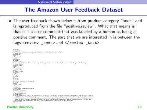
The user feedback shown below is from product category “book” andis reproduced from the file “positive.review”. What that means isthat it is a user comment that was labeled by a human as being apositive comment. The part that we are interested in is between thetags <review _text> and </review _text>.

<review><unique_id>188105201X:excellent_resource_for_principals!:[email protected]</unique_id><unique_id>3294</unique_id><asin>188105201X</asin><product_name>Leadership and the New Science: Learning About Organization from an Orderly Universe: Books: Margaret J. Wheatley</product_name><product_type>books</product_type><product_type>books</product_type><helpful>3 of 3</helpful><rating>5.0</rating><title>Excellent resource for principals!</title><date>July 6, 1999</date><reviewer>[email protected]</reviewer><reviewer_location>Milwaukee, Wisconsin</reviewer_location><review_text>I am ordering copies for all 23 middle school principals and the two assistant principals leading two middle school programsin the Milwaukee Public Schools system. We will use Wheatley’s book as the primary resource for our professional growth atour MPS Middle School Principals Collaborative institute August 9-11, 1999. We are not just concerned with reform; we seekrenewal as well. Wheatley provides the basis. She notes that Einstein said that a problem cannot be solved from the sameconsciousness that created it. The entire book is a marvelous exploration of this philosophy

</review_text></review>

Purdue University 10


The Amazon User Feedback Dataset (contd.)

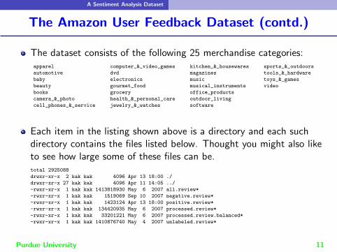
The dataset consists of the following 25 merchandise categories:apparel computer_&_video_games kitchen_&_housewares sports_&_outdoors

automotive dvd magazines tools_&_hardware

baby electronics music toys_&_games

beauty gourmet_food musical_instruments video

books grocery office_products

camera_&_photo health_&_personal_care outdoor_living

cell_phones_&_service jewelry_&_watches software

Each item in the listing shown above is a directory and each suchdirectory contains the files listed below. Thought you might also liketo see how large some of these files can be.total 2925088

drwxr-xr-x 2 kak kak 4096 Apr 13 18:00 ./

drwxr-xr-x 27 kak kak 4096 Apr 11 14:05 ../

-rwxr-xr-x 1 kak kak 1413818930 May 6 2007 all.review*

-rwxr-xr-x 1 kak kak 1519069 Sep 10 2007 negative.review*

-rwxr-xr-x 1 kak kak 1423124 Apr 13 18:00 positive.review*

-rwxr-xr-x 1 kak kak 134420935 May 6 2007 processed.review*

-rwxr-xr-x 1 kak kak 33201221 May 6 2007 processed.review.balanced*

-rwxr-xr-x 1 kak kak 1410876740 May 4 2007 unlabeled.review*



The Amazon User Feedback Dataset (contd.)

Our interest is primarily in the files positive.reviews andnegative.reviews. If you’d like to know how many reviews are therein each of these two files, that information is provided in a file namedsummary.txt in the same directory that has all the product categories:apparel/negative.review 1000apparel/positive.review 1000apparel/unlabeled.review 7252automotive/negative.review 152automotive/positive.review 584baby/negative.review 900baby/positive.review 1000baby/unlabeled.review 2356beauty/negative.review 493beauty/positive.review 1000beauty/unlabeled.review 1391books/negative.review 1000books/positive.review 1000books/unlabeled.review 973194camera & photo/negative.review 999camera & photo/positive.review 1000camera & photo/unlabeled.review 5409cell phones & service/negative.review 384cell phones & service/positive.review 639computer & video games/negative.review 458computer & video games/positive.review 1000computer & video games/unlabeled.review 1313dvd/negative.review 1000dvd/positive.review 1000dvd/unlabeled.review 122438electronics/negative.review 1000electronics/positive.review 1000electronics/unlabeled.review 21009gourmet food/negative.review 208gourmet food/positive.review 1000gourmet food/unlabeled.review 367grocery/negative.review 352grocery/positive.review 1000grocery/unlabeled.review 1280health & personal care/negative.review 1000health & personal care/positive.review 1000health & personal care/unlabeled.review 5225jewelry & watches/negative.review 292jewelry & watches/positive.review 1000jewelry & watches/unlabeled.review 689kitchen & housewares/negative.review 1000kitchen & housewares/positive.review 1000kitchen & housewares/unlabeled.review 17856magazines/negative.review 970magazines/positive.review 1000magazines/unlabeled.review 2221music/negative.review 1000music/positive.review 1000music/unlabeled.review 172180musical instruments/negative.review 48musical instruments/positive.review 284office products/negative.review 64office products/positive.review 367outdoor living/negative.review 327outdoor living/positive.review 1000outdoor living/unlabeled.review 272software/negative.review 915software/positive.review 1000software/unlabeled.review 475sports & outdoors/negative.review 1000sports & outdoors/positive.review 1000sports & outdoors/unlabeled.review 3728tools & hardware/negative.review 14tools & hardware/positive.review 98toys & games/negative.review 1000toys & games/positive.review 1000toys & games/unlabeled.review 11147video/negative.review 1000video/positive.review 1000video/unlabeled.review 34180




Version 1.1.4 of DLStudio comes with the following text datasetarchive files:

sentiment_dataset_train_400.tar.gz vocab_size = 64,350

sentiment_dataset_test_400.tar.gz





The archive names with, say, ’400’ in them were made using the first400 positive and 400 negative comments in each of the 25 productcategories. The reviews thus collected are randomized and dividedinto the training and the testing datasets in 80:20 ratio.

When you download the above two datasets, you will also get thefollowing two files:



These are to help you debug your code quickly.Purdue University 13

An RNN That Predicts the Ethnic Origin of a Last Name

Outline










A Simple (But Fun) Example of a Neural Networkwith Feedback

This example in a tutorial by Sean Robertson has got to be one of themost wonderful illustrations of how much fun you can have with aneural network that incorporates feedback. Here is a link to thisexample:

https://pytorch.org/tutorials/intermediate/char_rnn_classification_tutorial.html

The goal is to predict the ethnic origin of a last name.

Figure: A Recurrent Neural Network for Predicting the Nationality of a Last Name


https://pytorch.org/tutorials/intermediate/char_rnn_classification_tutorial.html


A Simple But Fun Example of RNN (contd.)

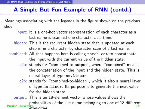
Meanings associating with the legends in the figure shown on the previousslide:

input: It is a one-hot vector representation of each character as alast name is scanned one character at a time.

hidden: This is the recurrent hidden state that is updated at eachstep in in a character-by-character scan of a last name.

combined: All that happens here is calling torch.cat to concatenatethe input with the current value of the hidden state.

c2o: stands for “combined-to-output”, where “combined” meansthe concatenation of the input and the hidden state. This isneural layer of type nn.Linear.

c2h: stands for “combined-to-hidden”, which is also a neural layerof type nn.Liner. Its purpose is to generate the next valuefor the hidden state.

output: This is an 18-element vector whose values shows theprobabilities of the last name belonging to one of 18 differentethnicities.



Predicting the Ethnicity of a Last Name

Each loop of training in the code for this example does the following:1 Create the input tensor for the last name and a tensor for the output

ethnicity2 Create a zeroed initial hidden state3 Scan the last name one character at a time and feed its one-hot vector

at the input4 Update the hidden state for the next character in the last name5 Compare the final output to the target ethnicity6 Backpropagate7 Return the output and loss

The important thing to note that the hidden state is initialized tozeros for each new training sample, meaning for each new last nameand its associated ethnic origin.

All the last names for a given ethnicity are placed in a single file andthe name of the file designates the ethnic origin of the names in thatfile.



The Network

Shown below is code that defines the network depicted on Slide 15.

The size of the input is dictated by the number of printable asciicharacters (without including the digits, etc.)

The size of the hidden state was set experimentally.

class RNN(nn.Module):

def __init__(self, input_size, hidden_size, output_size):

super(RNN, self).__init__()

self.hidden_size = hidden_size

# input_size=57 hidden_size=128

self.c2h = nn.Linear(input_size + hidden_size, hidden_size)

# output_size=18

self.c2o = nn.Linear(input_size + hidden_size, output_size)

self.softmax = nn.LogSoftmax(dim=1)

def forward(self, input, hidden):

combined = torch.cat((input, hidden), 1)

hidden = self.c2h(combined)

output = self.c2o(combined)

output = self.softmax(output)

return output, hidden



Some Utility Functions

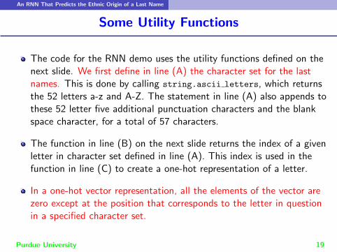
The code for the RNN demo uses the utility functions defined on thenext slide. We first define in line (A) the character set for the lastnames. This is done by calling string.ascii letters, which returnsthe 52 letters a-z and A-Z. The statement in line (A) also appends tothese 52 letter five additional punctuation characters and the blankspace character, for a total of 57 characters.

The function in line (B) on the next slide returns the index of a givenletter in character set defined in line (A). This index is used in thefunction in line (C) to create a one-hot representation of a letter.

In a one-hot vector representation, all the elements of the vector arezero except at the position that corresponds to the letter in questionin a specified character set.



Some Utility Functions (contd.)

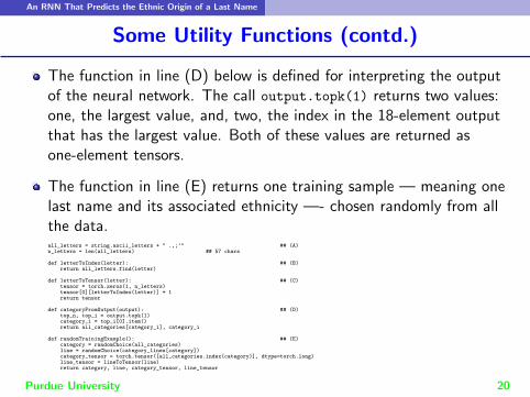
The function in line (D) below is defined for interpreting the outputof the neural network. The call output.topk(1) returns two values:one, the largest value, and, two, the index in the 18-element outputthat has the largest value. Both of these values are returned asone-element tensors.

The function in line (E) returns one training sample — meaning onelast name and its associated ethnicity —- chosen randomly from allthe data.all_letters = string.ascii_letters + " .,;’" ## (A)n_letters = len(all_letters) ## 57 chars

def letterToIndex(letter): ## (B)return all_letters.find(letter)

def letterToTensor(letter): ## (C)tensor = torch.zeros(1, n_letters)tensor[0][letterToIndex(letter)] = 1return tensor

def categoryFromOutput(output): ## (D)top_n, top_i = output.topk(1)category_i = top_i[0].item()return all_categories[category_i], category_i

def randomTrainingExample(): ## (E)category = randomChoice(all_categories)line = randomChoice(category_lines[category])category_tensor = torch.tensor([all_categories.index(category)], dtype=torch.long)line_tensor = lineToTensor(line)return category, line, category_tensor, line_tensor



The train() Function

Note how the basic training function carries out the iterationsinvolved in scanning the input last name one character at a time.

Also, instead of using epochs, in this case, we will simply selectrandomly from all the training data and do so as many times as wewish for achieving basically the same effect that you get by trainingover several epochs.

criterion = nn.NLLLoss()

learning_rate = 0.005

def train(category_tensor, line_tensor):

hidden = rnn.initHidden()

rnn.zero_grad() ## zeros out the gradients for learnable params

for i in range(line_tensor.size()[0]):

output, hidden = rnn(line_tensor[i], hidden)

loss = criterion(output, category_tensor)

loss.backward()

for p in rnn.parameters():

p.data.add_(-learning_rate, p.grad.data)

return output, loss.item()



The train() Function (contd.)

About the loss function nn.NLLLoss(), it stands for “Negative LogLikelihood Loss”. This is the loss function to use if the output of yournetwork is produced by a nn.LogSoftmax layer.

The nn.NLLLoss() loss function expects at its input log-probabilitiesfor the different classes — such as those produced by nn.LogSoftmax.

One can show theoretically that the combined effect ofnn.LogSoftmax in the output of a network and nn.NLLLoss() for lossis exactly the same as using CrossEntropyLoss for loss.

For iterative training, we repeated call train() a large number oftimes over the training dataset as shown below

The variable line tensor is the tensor representation of the lastname in a training file. If a last name has, say, 5 characters, thistensor has shape (5, 57).


Solving the Problem of Sentiment Analysis

Outline










A Recurrent Network for Sentiment Analysis

This section presents an attempt at solving the sentiment analysisproblem. Shown on the next slide are some of the utility functions forthis exercise.

First we must define the functions that convert the text into tensorrepresentations. Toward that end, as shown by the function whosedefinition starts at line (A) on Slide 26, each word is given a one-hotrepresentation that, as you would expect, depends on the size of thevocabulary (which, by the way, comes with the datasets that Iprovide).

The size of the vocabulary is 17,001 if you only scrape 40 positivereviews and an equal number of negative reviews from each productcategory. However, the size of the vocabulary goes up to 43,285 whenthe number of reviews collected for each product type is 400. For thissized vocabulary, the one-hot representation for a word will involvetensors that are as large as 43,285.



A Recurrent Network for Sentiment Analysis(contd.)

To continue from the previous slide, and if a review has a couple ofhundred words in it (not uncommon), you are looking at the tensorrepresentation of a review whose shape could be (200, 43285)

The tensor representation of a review is generated by the functionwhose definition starts in line (B) on the next slide.

We also need to convert the sentiment associated with a review into atensor. In the dataset that I provide, the negative sentiment isrepresented by the integer 0 and the positive by the integer 1. Thefunction whose definition starts in line (C) on the next slide does thejob of converting these numbers into tensors.

The functions in lines (D) and (E) are the required functions for thecustom dataloader.



The Utility Functions

def one_hotvec_for_word(self, word): ## (A)word_index = self.vocab.index(word)hotvec = torch.zeros(1, len(self.vocab))hotvec[0, word_index] = 1return hotvec

def review_to_tensor(self, review): ## (B)review_tensor = torch.zeros(len(review), len(self.vocab))for i,word in enumerate(review):

review_tensor[i,:] = self.one_hotvec_for_word(word)return review_tensor

def sentiment_to_tensor(self, sentiment): ## (C)"""Sentiment is ordinarily just a binary valued thing. It is 0 for negativesentiment and 1 for positive sentiment. We need to pack this value in atwo-element tensor."""sentiment_tensor = torch.zeros(2)if sentiment is 1:

sentiment_tensor[1] = 1elif sentiment is 0:

sentiment_tensor[0] = 1sentiment_tensor = sentiment_tensor.type(torch.long)return sentiment_tensor

def __len__(self): ## (D)if self.train_or_test is ’train’:

return len(self.indexed_dataset_train)elif self.train_or_test is ’test’:

return len(self.indexed_dataset_test)

def __getitem__(self, idx): ## (E)sample = self.indexed_dataset_train[idx] if self.train_or_test is ’train’ else self.indexed_dataset_test[idx]review = sample[0]review_category = sample[1]review_sentiment = sample[2]review_sentiment = self.sentiment_to_tensor(review_sentiment)review_tensor = self.review_to_tensor(review)category_index = self.categories.index(review_category)sample = {’review’ : review_tensor,

’category’ : category_index, # should be converted to tensor, but not yet used’sentiment’ : review_sentiment }

return sample



Sentiment Analysis Network

Shown below is a vanilla implementation of a network for sentimentanalysis — it does not lend itself to the use of any gates forprotecting against the vanishing or exploding gradients.

class TEXTnet(nn.Module):

def __init__(self, input_size, hidden_size, output_size):

super(DLStudio.TextClassification.TEXTnet, self).__init__()

self.input_size = input_size


self.output_size = output_size

self.combined_to_hidden = nn.Linear(input_size + hidden_size, hidden_size)

self.combined_to_middle = nn.Linear(input_size + hidden_size, 100)

self.middle_to_out = nn.Linear(100, output_size)

self.logsoftmax = nn.LogSoftmax(dim=1)

self.dropout = nn.Dropout(p=0.1)

def forward(self, input, hidden):

combined = torch.cat((input, hidden), 1)

hidden = self.combined_to_hidden(combined)

out = self.combined_to_middle(combined)

out = torch.nn.functional.relu(out)

out = self.dropout(out)

out = self.middle_to_out(out)

out = self.logsoftmax(out)

return out,hidden



The TEXTnet Network

The network defined on the previous slide is shown below:

Figure: A Recurrent Neural Network for Semantic Analysis of Text



The Training Function Used for the TEXTnet Network

In the training code that follows note how in line (A) we reinitializethe hidden state to all zeros for each review.

Note how a review, which may consist of any number of words, isscanned one word at a time in lines (B), (C), and (D) and how theone-hot vector for each new word is combined with the value of thehidden that summarizes all the words seen previously in that review.def run_code_for_training_with_TEXTnet_no_gru(self, net, hidden_size):

net = net.to(self.dl_studio.device)criterion = nn.NLLLoss()optimizer = optim.SGD(net.parameters(), lr=self.dl_studio.learning_rate, momentum=self.dl_studio.momentum)start_time = time.clock()for epoch in range(self.dl_studio.epochs):

running_loss = 0.0for i, data in enumerate(self.train_dataloader):

hidden = torch.zeros(1, hidden_size) ## (A)hidden = hidden.to(self.dl_studio.device)review_tensor,category,sentiment = data[’review’], data[’category’], data[’sentiment’]review_tensor = review_tensor.to(self.dl_studio.device)sentiment = sentiment.to(self.dl_studio.device)optimizer.zero_grad()input = torch.zeros(1,review_tensor.shape[2])input = input.to(self.dl_studio.device)for k in range(review_tensor.shape[1]): ## (B)

input[0,:] = review_tensor[0,k] ## (C)output, hidden = net(input, hidden) ## (D)

loss = criterion(output, torch.argmax(sentiment,1))running_loss += loss.item()loss.backward(retain_graph=True)optimizer.step()if i % 100 == 99:

avg_loss = running_loss / float(100)current_time = time.clock()time_elapsed = current_time-start_timeprint("[epoch:%d iter:%4d elapsed_time: %4d secs] loss: %.3f" % (epoch+1,i+1, time_elapsed,avg_loss))running_loss = 0.0

self.save_model(net)



The Testing Function Used for the TEXTnet Network

As in the training function, in the testing function also we reinitializein line (A) the hidden state to all zeros for each new unseen review.

In lines (B), (C), and (D), the review is scanned one word at a timeand, for each new word, its one-hot vector concatenated with thehidden state that represents all the words seen preiously in the review.def run_code_for_testing_with_TEXTnet_no_gru(self, net, hidden_size):

net.load_state_dict(torch.load(self.dl_studio.path_saved_model))negative_total = 0positive_total = 0confusion_matrix = torch.zeros(2,2)with torch.no_grad():

for i, data in enumerate(self.test_dataloader):review_tensor,category,sentiment = data[’review’], data[’category’], data[’sentiment’]input = torch.zeros(1,review_tensor.shape[2])hidden = torch.zeros(1, hidden_size) ## (A)for k in range(review_tensor.shape[1]): ## (B)

input[0,:] = review_tensor[0,k] ## (C)output, hidden = net(input, hidden) ## (D)

predicted_idx = torch.argmax(output).item()gt_idx = torch.argmax(sentiment).item()if i % 100 == 99:

print(" [i=%4d] predicted_label=%d gt_label=%d" % (i+1, predicted_idx,gt_idx))if gt_idx is 0:

negative_total += 1elif gt_idx is 1:

positive_total += 1confusion_matrix[gt_idx,predicted_idx] += 1

out_percent = np.zeros((2,2), dtype=’float’)out_percent[0,0] = "%.3f" % (100 * confusion_matrix[0,0] / float(negative_total))out_percent[0,1] = "%.3f" % (100 * confusion_matrix[0,1] / float(negative_total))out_percent[1,0] = "%.3f" % (100 * confusion_matrix[1,0] / float(positive_total))out_percent[1,1] = "%.3f" % (100 * confusion_matrix[1,1] / float(positive_total))print("\n\nDisplaying the confusion matrix:\n")out_str = " "out_str += "%18s %18s" % (’predicted negative’, ’predicted positive’)print(out_str + "\n")for i,label in enumerate([’true negative’, ’true positive’]):

out_str = "%12s: " % labelfor j in range(2):

out_str += "%18s" % out_percent[i,j]print(out_str)Purdue University 30


Results Obtained with the TEXTnet Network

The results shown on this slide are based on the following datasetthat was described earlier on Slide 13:

sentiment_dataset_train_40.tar.gz


Using one epoch of training, shown below is the confusion matrix thatis produced by the network presented on the previous two slides withthe learning rate set to 10−5:

Number of unseen positive reviews tested: 200

Number of unseen negative reviews tested: 195

Displaying the confusion matrix:

predicted negative predicted positive

true negative: 0.0 100.0

true positive: 0.0 100.0

These results were produced by Python 3 execution of the scripttext classification with TEXTnet no gru.py in the Examples directory of DLStudio,Version 1.1.4.



Results with the TEXTnet Network (contd.)

The dismal results shown on the previous slide are, in all likelihood, aresult of a combination of the vanishing gradients and the very smallsize of the training data.

These poor results are in keeping with the fact that, as shown below,the loss does not exhibit any decrease with training:

[epoch:1 iter: 100 elapsed_time: 26 secs] loss: 0.693[epoch:1 iter: 200 elapsed_time: 61 secs] loss: 0.694[epoch:1 iter: 300 elapsed_time: 94 secs] loss: 0.694[epoch:1 iter: 400 elapsed_time: 133 secs] loss: 0.692[epoch:1 iter: 500 elapsed_time: 164 secs] loss: 0.696[epoch:1 iter: 600 elapsed_time: 197 secs] loss: 0.693[epoch:1 iter: 700 elapsed_time: 228 secs] loss: 0.692[epoch:1 iter: 800 elapsed_time: 254 secs] loss: 0.693[epoch:1 iter: 900 elapsed_time: 288 secs] loss: 0.690[epoch:1 iter:1000 elapsed_time: 322 secs] loss: 0.694[epoch:1 iter:1100 elapsed_time: 358 secs] loss: 0.694[epoch:1 iter:1200 elapsed_time: 394 secs] loss: 0.694[epoch:1 iter:1300 elapsed_time: 427 secs] loss: 0.694[epoch:1 iter:1400 elapsed_time: 466 secs] loss: 0.694[epoch:1 iter:1500 elapsed_time: 501 secs] loss: 0.690

AN IMPORTANT NOTE: About the role played by the small size of the training dataset (which has only 40 positive

and 40 negative reviews for each product category) in the results presented on the previous slide, note that its

vocabulary size as shown in Slide 13 is 17,001. This would also be the size of the one-hot vectors for the words. If we

were to use the larger datasets mentioned on that slide, the size of the one-hot vectors would go up also, which would

increase the number of learnable parameters, and that, in turn, would create a need for a still larger dataset. This is a

catch-22 situation that can only be solved by using, say, the fixed-size word embeddings for the words (see the Week 14

slides) as opposed to the one-hot vectors.



A Stepping Stone to Gating — The TEXTnetOrder2 Network

Shown on the next slide is an attempt at making stronger thefeedback mechanism in TEXTnet by incorporating in it the value ofthe hidden state at the previous time step.

The third parameter ’cell’ in the definition of forward()’ plays animportant role in how TEXTnetOrder2 lends itself to somerudimentary gating action. See the explanation for the trainingfunction for why that is the case.

As shown in line (C), the current value of hidden is processed by alinear layer, followed by the sigmoid nonlinearity, for its storage in theoutgoing value of cell.

The network that results from the definition on the next slide isshown in Slide 35.



The TEXTnetOrder2 Network

class TEXTnetOrder2(nn.Module):

def __init__(self, input_size, hidden_size, output_size, dls):

super(DLStudio.TextClassification.TEXTnetOrder2, self).__init__()

self.input_size = input_size


self.output_size = output_size

self.combined_to_hidden = nn.Linear(input_size + 2*hidden_size, hidden_size)

self.combined_to_middle = nn.Linear(input_size + 2*hidden_size, 100)

self.middle_to_out = nn.Linear(100, output_size)


self.dropout = nn.Dropout(p=0.1)

# for the cell

self.linear_for_cell = nn.Linear(hidden_size, hidden_size) ## (A)

def forward(self, input, hidden, cell): ## (B)

combined = torch.cat((input, hidden, cell), 1)

hidden = self.combined_to_hidden(combined)

out = self.combined_to_middle(combined)

out = torch.nn.functional.relu(out)

out = self.dropout(out)

out = self.middle_to_out(out)


hidden_clone = hidden.clone()

cell = torch.sigmoid(self.linear_for_cell(hidden_clone)) ## (C)

return out,hidden,cell

def initialize_cell(self, batch_size):

weight = next(self.linear_for_cell.parameters()).data

cell = weight.new(1, self.hidden_size).zero_()

return cellPurdue University 34


The TEXTnetOrder2 Network (contd.)



The Training Function Used for the TEXTnetOrder2 Network

The local variables cell prev and cell prev 2 prev defined in lines(A) and (B) allow for the value of the hidden state at the previoustime step to be factored into the logic at the current time-step in line(F). As to how a review is scanned word by word is the same as forthe TEXTnet network. Also note how the hidden state is initialized toall zeros in line (C) for each product review.def run_code_for_training_with_TEXTnetOrder2_no_gru(self, net, hidden_size):

net = net.to(self.dl_studio.device)criterion = nn.NLLLoss()optimizer = optim.SGD(net.parameters(), lr=self.dl_studio.learning_rate, momentum=self.dl_studio.momentum)start_time = time.clock()for epoch in range(self.dl_studio.epochs):

running_loss = 0.0for i, data in enumerate(self.train_dataloader):

cell_prev = net.initialize_cell(1).to(self.dl_studio.device) ## (A)cell_prev_2_prev = net.initialize_cell(1).to(self.dl_studio.device) ## (B)hidden = torch.zeros(1, hidden_size) ## (C)hidden = hidden.to(self.dl_studio.device)review_tensor,category,sentiment = data[’review’], data[’category’], data[’sentiment’]review_tensor = review_tensor.to(self.dl_studio.device)sentiment = sentiment.to(self.dl_studio.device)optimizer.zero_grad()input = torch.zeros(1,review_tensor.shape[2])input = input.to(self.dl_studio.device)for k in range(review_tensor.shape[1]): ## (D)

input[0,:] = review_tensor[0,k] ## (E)output, hidden, cell = net(input, hidden, cell_prev_2_prev) ## (F)if k == 0: ## (G)

cell_prev = cell ## (H)else: ## (I)

cell_prev_2_prev = cell_prev ## (J)cell_prev = cell ## (K)

loss = criterion(output, torch.argmax(sentiment,1))running_loss += loss.item()loss.backward()optimizer.step()if i % 100 == 99:

avg_loss = running_loss / float(100)current_time = time.clock()time_elapsed = current_time-start_timeprint("[epoch:%d iter:%4d elapsed_time: %4d secs] loss: %.3f" % (epoch+1,i+1, time_elapsed,avg_loss))running_loss = 0.0

self.save_model(net)Purdue University 36


The Testing Function Used for the TEXTnetOrder2 Network

Like the training function shown on the previous slide, the testingfunction also uses the local variables cell prev andcell prev 2 prev defined in lines (A) and (B) to allow for the valueof the hidden state at the previous time step to be factored into thelogic at the current time-step in line (D).def run_code_for_testing_with_TEXTnetOrder2_no_gru(self, net, hidden_size):

net.load_state_dict(torch.load(self.dl_studio.path_saved_model))negative_total = 0positive_total = 0confusion_matrix = torch.zeros(2,2)with torch.no_grad():

for i, data in enumerate(self.test_dataloader):cell_prev = net.initialize_cell(1) ## (A)cell_prev_2_prev = net.initialize_cell(1) ## (B)review_tensor,category,sentiment = data[’review’], data[’category’], data[’sentiment’]input = torch.zeros(1,review_tensor.shape[2])hidden = torch.zeros(1, hidden_size) ## (C)for k in range(review_tensor.shape[1]):

input[0,:] = review_tensor[0,k]output, hidden, cell = net(input, hidden, cell_prev_2_prev) ## (D)if k == 0: ## (E)

cell_prev = cell ## (F)else: ## (G)

cell_prev_2_prev = cell_prev ## (H)cell_prev = cell ## (I)

predicted_idx = torch.argmax(output).item()gt_idx = torch.argmax(sentiment).item()if gt_idx is 0:



out_percent = np.zeros((2,2), dtype=’float’)out_percent[0,0] = "%.3f" % (100 * confusion_matrix[0,0] / float(negative_total))out_percent[0,1] = "%.3f" % (100 * confusion_matrix[0,1] / float(negative_total))out_percent[1,0] = "%.3f" % (100 * confusion_matrix[1,0] / float(positive_total))out_percent[1,1] = "%.3f" % (100 * confusion_matrix[1,1] / float(positive_total))out_str = " "out_str += "%18s %18s" % (’predicted negative’, ’predicted positive’)print(out_str + "\n")for i,label in enumerate([’true negative’, ’true positive’]):


out_str += "%18s" % out_percent[i,j]print(out_str)Purdue University 37


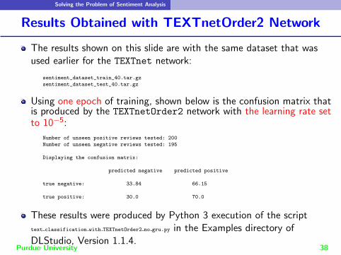
Results Obtained with TEXTnetOrder2 Network

The results shown on this slide are with the same dataset that wasused earlier for the TEXTnet network:

sentiment_dataset_train_40.tar.gz


Using one epoch of training, shown below is the confusion matrix thatis produced by the TEXTnetOrder2 network with the learning rate setto 10−5:

Number of unseen positive reviews tested: 200

Number of unseen negative reviews tested: 195

Displaying the confusion matrix:

predicted negative predicted positive

true negative: 33.84 66.15

true positive: 30.0 70.0

These results were produced by Python 3 execution of the scripttext classification with TEXTnetOrder2 no gru.py in the Examples directory ofDLStudio, Version 1.1.4.

These results are still poor. Therefore, we have no choice but to diginto the material that follows in this lecture.


Gating Mechanisms to Deal with the Problem of VanishingGradients in RNNs

Outline










Why We Need the Gating Mechanisms

For non-trivial problems, the backpropagation of loss in an RNNinvolves long chains of dependencies because it must span all previousvalues of the hidden state that contributed to the present value at theoutput.

This leads to an even more challenging version of the vanishinggradients problem that you saw earlier in deep neural networks (withno feedback).

In the chains of dependencies created by feedback, the short-termdependencies can completely dominate the long-term dependencies,which basically negates what you had hoped to achieve with feedback.

In the literature you will find two commonly used gating mechanismsto deal with the vanishing gradients problem in RNNs: LSTM (LongShort-Term Memory) and GRU (Gated Recurrent Unit), with thelatter being the more recent.



The Basic Idea of Gating

The basic idea of a gating mechanism is that you designate a specialvariable (usually referred to as the cell) that is the keeper ofinformation from the past. What was placed in the cell is subject tobeing forgotten if it is not so relevant to the current state of theinput/output relationship. At the same time, the cell can be updatedbased on the current input/output relationship if that is deemed to beimportant for future characterizations of the input.

The previous slide mentioned the two most commonly used gatedRNNs as GRUs and LSTMs. Here is a wonderful paper by Chung etal. that has carried out a comparative evaluation of the two:

https://arxiv.org/abs/1412.3555

In the rest of this section, I’ll first present some preliminary conceptsdrawn from the above paper, which will be followed by an explanationof the structure of a GRU.




The Hidden State and its Evolution

Let’s denote the input sequence that is scanned by the network oneelement at a time by

X = (x1, x2, . . . , xT )

In general, any joint distribution over these T variables can bedecomposed in the following manner:

p(x1, . . . , xT ) = p(x1)p(x2|x1)p(x3|x1, x2) . . . p(xT |x1, . . . , xT−1)

Let’s say that we can postulate the existence of a variable, denotedht , that allows us to write the following form for any of thecomponent distributions shown at right above:

p(xt |x1, . . . , xt−1) = φ(ht)

where φ() is a bounded and differentiable function like certainactivation functions such as the sigmoid and the hyperbolic tangentfunction (nn.tanh()).Purdue University 42


The Hidden State and its Evolution (contd.)

The relationship at the bottom of the previous slide says that ourvariable length input sequence xi is such that the probabilisticdependence of each sample on all the previous samples is dictated bythe time evolution of a specific fixed-sized entity ht through abounded and differentiable φ().

Input sequences that admit ht ’s that obey the condition presented onthe previous slide can be processed by the gating mechanisms such asGRU and LSTM for the remediation of the vanishing gradientsproblem. The function ht is referred to as the hidden state of thenetwork at time step t.

The explanation so far has focused on how an input sequence may begenerated from the time evolution of a hidden state. However, thatimplies the assumption that we are already in possession of the hiddenstate at time steps t. [By the way, that’s exactly what happens in the encoder-decoder frameworks

used in neural-network based approaches to machine translation: The encoder learns the fixed-sized hidden state for a

given input sentence in one language and the decoder maps that hidden state to a sentence in the target language.]




The last bullet on the previous slide begs the question: How togenerate the hidden state in the first place? Since the “job” of thehidden state is to generate the input sequence, and considering thedifferentiability and the boundedness assumptions we made in therelationship between xi and ht , the following form for learning thehidden state seems reasonable:

ht =

{0, t = 0

g(W xt + Uht−1), otherwise

where g() is again a bounded and differentiable function as beforeand where W and U are the matrices of learnable parameters.

The important thing to focus on in the equation shown above thatthe value of the hidden state at time-step t depends nonlinearly on itsvalue at the previous time-step t − 1.




If you couple the insight presented at the bottom of the previous slidewith the feedback diagram presented on Slide 15, you can see thatwith our new model for the input sequence and for the time evolutionof the hidden state, each element of the output sequence in thatdiagram will acquire a longer-range dependence on the current andthe previous samples of the input sequence. That’s one element ofwhat powers gated RNNs: A gated RNN can choose to forget thepast (and to possibly give greater emphasis to the present) over alonger range of dependencies into the past. The act of forgetting andresetting can be implemented with the help of gates as you will see inthe next section.

In the next few slides, let’s see how the GRU exploits the modelpresented here for its gating action.


Gated Recurrent Unit (GRU)

Outline










GRU — Reset and Update Gates

I’ll now focus on GRUs (Gated Recurrent Unit) in the rest of thediscussion here. GRUs were first proposed in the paper by Cho et el.that you can access through the following link:


Shown in the figure below is a high-level diagrammatic representationof a GRU. Basically, it has two “gates”, denoted r and z that standfor the reset gate and the update gate. As to why they are referred toas “gates” will become clear shortly.

Figure: This figure, taken from the GRU vs. LSTM comparative evaluation paper cited earlier, is a pictorial

depiction of a GRU. The reset and the update gates of a GRU are show as r and z in the figure, whereas h and h̃ arethe current value for the hidden state and a candidate value for the same.




GRU – Updating the Hidden State

The input into a GRU consists of the ongoing values for the sequencesx and h where the latter represents the hidden state for the former.

The figure shown on the previous slide seeks to depict the followingrelationship between the value of the hidden state at time-step t andthe same at time-step t − 1:

hjt = (1− z jt )hjt−1 + z jt h̃jt

where hjt is the j th element of the vector ht and where the updategate z jt is given by

z jt = σ(Wzxt + Uzht−1)j

where σ is a logistic sigmoid function given by σ(x) = 11+exp−x . It

smoothly rises from 0 to 1 over its entire domain. Its value at x = 0is 0.5. Wz and Uz are matrices of learnable parameters for the updategate.



Why Call it a Gate?

With regard to the last equation shown on the previous slide, note theimplications of the logistic sigmoid nonlinearity with regard to howeach component of h gets updated.

Just for illustration, assume that the argument to the σ() is such thatit is either sufficient negative or sufficiently positive so that theoutput of σ() is either 0 or 1.

When σ() returns 0, for that component of h, the update gate willevaluate to 0 and, therefore, the previous value of the hidden statewill dominate its current value.

On the other hand, should σ() return 1, the previous value for thehidden state will be ignored and the new value for the hidden statewill be dominated by h̃t . That should explain why we may refer to ztas a gate that decides the fate of each component of h separately.But what is h̃t?



GRU – Equation for the Reset Gate

The new thing h̃t that you see in the update equation for z jt dependson the current value for the sequence x and the previous value for thehidden state ht−1 but as modulated by another gate known as thereset gate:

h̃jt = tanh(Whxt + Uh(rt � ht−1))j

where � represents an element-wise multiplication. As you surelyknow already, tanh(x) is another one of those famous activationfunctions for neural networks. In its appearance, it is very much likethe logistic sigmoid except that it saturates out at -1 at the low endend +1 at the high end. As was the case earlier with similar entities,Wh and Uh are matrices of learnable parameters.

About the reset gate r shown above, it is given by

r jt = σ(Wrxt + Urht−1)j



GRU – The Gate Semantics

In the description of a GRU on the previous slides, notice how themathematical forms shown force the update and the reset semanticson the values calculated as z and r. The fact that z’s role is that ofupdating the hidden state should be obvious from the first equationon Slide 42. The role of the r gate as that of resetting the hiddenstate should also be obvious.

Shown below is a pictorial depiction of the network that incorporatesall of the GRU related equations shown so far. This picture is from:

https://blog.floydhub.com/gru-with-pytorch/

Figure: The network is a composite depiction created from the GRU update and reset equations presented.


https://blog.floydhub.com/gru-with-pytorch/


The GRU (contd.)

The blog cited in the previous slide contains an interesting exampleon the modeling of sequential data: the example is based on thesequences of energy consumption data at several power distributioncenters in the US. The goal is to create a “language model” for thesequences and then use the model to predict the energy consumptionat the next time step.

Using RNNs to create a language model is a big part of the modernneural-network based algorithms for automatic translation from onelanguage to another. I believe the more recent versions of the GoogleTranslate app are powered by such algorithms.


The GRUnet Class in the DLStudio Module

Outline










The GRUnet class in DLStudio

Shown below is the GRUnet class in the inner classTextClassification of the DLStudio module. Except for the factthat the output in forward() is routed through a LogSoftmaxactivation, it is the same as what you’ll find in Gabriel Loye’s GitHubcode for the example I mentioned on Slides 51 and 52.

class GRUnet(nn.Module):

def __init__(self, input_size, hidden_size, output_size, n_layers, drop_prob=0.2):

super(DLStudio.TextClassification.GRUnet, self).__init__()


self.n_layers = n_layers

self.gru = nn.GRU(input_size, hidden_size, n_layers, batch_first=True, dropout=drop_prob)

self.fc = nn.Linear(hidden_size, output_size)

self.relu = nn.ReLU()


def forward(self, x, h):

out, h = self.gru(x, h)

out = self.fc(self.relu(out[:,-1]))


return out, h

def init_hidden(self, batch_size):

weight = next(self.parameters()).data

hidden = weight.new(self.n_layers, batch_size, self.hidden_size).zero_()

return hidden



Training with the GRUnet Class

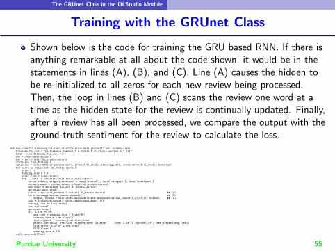
Shown below is the code for training the GRU based RNN. If there isanything remarkable at all about the code shown, it would be in thestatements in lines (A), (B), and (C). Line (A) causes the hidden tobe re-initialized to all zeros for each new review being processed.Then, the loop in lines (B) and (C) scans the review one word at atime as the hidden state for the review is continually updated. Finally,after a review has all been processed, we compare the output with theground-truth sentiment for the review to calculate the loss.

def run_code_for_training_for_text_classification_with_gru(self, net, hidden_size):filename_for_out = "performance_numbers_" + str(self.dl_studio.epochs) + ".txt"FILE = open(filename_for_out, ’w’)net = copy.deepcopy(net)net = net.to(self.dl_studio.device)criterion = nn.NLLLoss()optimizer = optim.SGD(net.parameters(), lr=self.dl_studio.learning_rate, momentum=self.dl_studio.momentum)for epoch in range(self.dl_studio.epochs):

print("")running_loss = 0.0start_time = time.clock()for i, data in enumerate(self.train_dataloader):

review_tensor,category,sentiment = data[’review’], data[’category’], data[’sentiment’]review_tensor = review_tensor.to(self.dl_studio.device)sentiment = sentiment.to(self.dl_studio.device)optimizer.zero_grad()hidden = net.init_hidden(1).to(self.dl_studio.device) ## (A)for k in range(review_tensor.shape[1]): ## (B)

output, hidden = net(torch.unsqueeze(torch.unsqueeze(review_tensor[0,k],0),0), hidden) ## (C)loss = criterion(output, torch.argmax(sentiment, 1))running_loss += loss.item()loss.backward()optimizer.step()if i % 100 == 99:

avg_loss = running_loss / float(99)current_time = time.clock()time_elapsed = current_time-start_timeprint("[epoch:%d iter:%3d elapsed_time: %d secs] loss: %.3f" % (epoch+1,i+1, time_elapsed,avg_loss))FILE.write("%.3f\n" % avg_loss)FILE.flush()running_loss = 0.0

self.save_model(net)



Testing with the GRUnet Class

As with the training script shown on the previous slide, we reinitializethe hidden state to all zeros in line (A) for each new unseen reviewused for testing. Each review is scanned word by word in the loop inlines (B) and (C) where the one-hot vector for each new word iscombined with the hidden state that represents all the previous wordsin the review.def run_code_for_testing_text_classification_with_gru(self, net, hidden_size):

net.load_state_dict(torch.load(self.dl_studio.path_saved_model))classification_accuracy = 0.0negative_total = 0positive_total = 0confusion_matrix = torch.zeros(2,2)with torch.no_grad():

for i, data in enumerate(self.test_dataloader):review_tensor,category,sentiment = data[’review’], data[’category’], data[’sentiment’]hidden = net.init_hidden(1) ## (A)for k in range(review_tensor.shape[1]): ## (B)

output, hidden = net(torch.unsqueeze(torch.unsqueeze(review_tensor[0,k],0),0), hidden) ## (C)predicted_idx = torch.argmax(output).item()gt_idx = torch.argmax(sentiment).item()if i % 100 == 99:

print(" [i=%d] predicted_label=%d gt_label=%d\n\n" % (i+1, predicted_idx,gt_idx))if predicted_idx == gt_idx:

classification_accuracy += 1if gt_idx is 0:



out_percent = np.zeros((2,2), dtype=’float’)out_percent[0,0] = "%.3f" % (100 * confusion_matrix[0,0] / float(negative_total))out_percent[0,1] = "%.3f" % (100 * confusion_matrix[0,1] / float(negative_total))out_percent[1,0] = "%.3f" % (100 * confusion_matrix[1,0] / float(positive_total))out_percent[1,1] = "%.3f" % (100 * confusion_matrix[1,1] / float(positive_total))print("\n\nNumber of positive reviews tested: %d" % positive_total)print("\n\nNumber of negative reviews tested: %d" % negative_total)print("\n\nDisplaying the confusion matrix:\n")out_str = " "out_str += "%18s %18s" % (’predicted negative’, ’predicted positive’)print(out_str + "\n")for i,label in enumerate([’true negative’, ’true positive’]):


out_str += "%18s" % out_percent[i,j]print(out_str)



How Come No Results with GRU?

Even with the smallest of the datasets listed on Slide 13, it takes 10times longer to train with the GRUnet than with TEXTnetOrder2.That is because of the size of the model created when using GRU.Shown below are the sizes of the GRU based models for the threedifferent datasets listed on Slide 13:

Size of GRU Based Model

dataset vocab size (in # of learnable params)

--------------- ---------- --------------------------

40-dataset 17,001 28,480,002

200-dataset 43,285 68,852,226

400-dataset 64,350 101,208,066

This display nicely summarizes why one-hot vectors is not the way togo for the numerical representations for words in a text corpus if theend-goal is to classify variable-length text.

As you increase the size of the dataset, the vocabulary size goes up,which makes the one-hot representations larger, and that, in turn,increases the size of the model, which creates a need for a still largerdataset. This is the catch-22 situation mentioned previously in thislecture that can only be remedied by using, say, word embeddings.Purdue University 57

Recurrent Neural Networks for Text Classi cation · Recurrent Neural Networks for Text Classi...

Documents

Transcript of Recurrent Neural Networks for Text Classi cation · Recurrent Neural Networks for Text Classi...