RECOVERY FROM THE 1930S GREAT DEPRESSION IN AUSTRALIA:A POLICY ANALYSIS BASED ON A CGE MODEL

Mahinda Siriwardana

May 1994

UNE Working Papers in Economics No. 10

Editor John Pullen

Department of EconomicsUniversity of New England

ArmidaleNew South Wales 2351

Australia

ISSN: 1321 - 9081

ISBN: 1 86389 185 4

RECOVERYFROM THE 1930S GREAT DEPRESSION IN AUSTRALIA : APOLICY ANALYSIS BASED ON A CGE MODEL

Mahinda Siriwardana*

University of New England

Mailing Address

Dr A. M. SiriwardanaDepartment of EconomicsUniversity of New EnglandArmidale, N.S.W. 2351Australia.

* I am grateful to Professor Peter Dixon for his valuable comments and advice during theformulation of the CGE model used in this study. Professors Malcolm Treadgold andMalcolm Falkus kindly read an earlier draft and made very useful suggestions. The paperalso benefited from comments made at the Annual Conference of Economists held at theMurdoch University, Perth, September 1993.

2

ABSTRACT

The striking similarities of economic problems facing Australia in the early1990s with those of the 1930s warrant a revisit to the recovery effort duringthe depression. This paper examines the effectiveness of various economicpolicies adopted to deal with the depression by simulating a computablegeneral equilibrium (CGE) model of the 1930s in Australia. The analysisfocuses on the relative importance of the exchange rate devaluation, theprotection policy, the government demand expansion and the wage policy. Italso evaluates the impact of alternative policies which would have provided adifferent outcome that may have been crucial to the recovery.

I Introduction

The depression of the 1930s influenced the economic activity of practically every countryand was a worldwide phenomenon. The severity and the duration of the depressionhowever differed from one country to another. Australia experienced a 10 per centdecline in its GDP between 1929 and 1931. Unemployment reached a record high levelby 1933, representing 19 per cent of the labour force in Australia (Gregory and Butlin,1988, pp.2-7).1 Domestic investment declined under the pressure of profits squeeze,collapse of the business confidence and more importantly, with the drying up of foreigncapital inflow. Australia’s terms of trade deteriorated by about 38 percent between 1929and 1932. The loss of export revenue immediately created balance of payments deficits,depressed national income levels and generated unmanageable budget deficits.2

These developments led to a debate in Australia in the early 1930s over the appropriategoals for economic policy and the mix of policy tools which should be adopted toachieve them. The economic policy making during the depression generally concentrated

upon reducing costs, minimising expenditure, curbing imports and stimulatinginvestment. The specific policies adopted in Australia to arrest the depression were theincrease in tariff protection, the devaluation, the budgetary policy towards balancedbudget, the lowering of interest rates and the reduction of real wages. These instrumentsreflect a mixture of contractionary and expansionary policies. However, it has beenargued that the deliberate policy measures have had relatively little effect towards thespeed of recovery (Schedvin, 1970; Valentine, 1988). This paper examines theeffectiveness of various economic policies used to deal with the depression by simulating

1 According to Trade Union Returns, the unemployment rate in Australia was 28 per centin 1932 (Schedvin, 1970, p.4).2 See Valentine (1987) and Siriwardana (1994) for a detailed analysis of the causes of thedepression in Australia.

3

a computable general equilibrium (CGE) model of the 1930s Australia.3 The analysisalso focuses on the impact of alternative policies which would have provided a different

outcome that may have been crucial to the recovery.

The paper is organised as follows. Section II provides an overview of the policy mix andthe consequent debate over the economic policy making in Australia during thedepression. This is required to put the ensuing analysis in a proper perspective. SectionI~ briefly outlines the CGE model used in the paper. Section IV describes the calibrationprocedure of the model and Section V sets out the simulations. The simulation results areanalysed in Section VI. Finally, Section VII summarises the main conclusions.

II The Policy Debate

It is generally believed that economic analysis played a minor role in formulating policiesduring the early 1930s in Australia. The newly elected Scullin government wasconfronted with a diversity of opinions emerged from politicians, economists and variousinterest groups. Though the initial response of the government to the depression wasexpansionary, the eventual policy package turned out to be basically contractionary. Thedebt repayment, the cutting of costs to improve the competitiveness, the balancing of thebudget and the restoration of Australia’s financial reputation were considered to be theprime goals of economic policies. These objectives eventually led to a wide range ofproposals to promote economic recovery (Spenceley, 1990).

The growing budget deficits of Commonwealth and State governments was a reflectionof the financial crisis fuelled by the deflationary effects of the depression. It created aserious political controversy leading to a clash within the members of the Labour Party

and between the banking system and the Labour government. The government had twoalternatives in relation to the budget, i.e. either to maintain the deficit at the existing levelor to adopt the balance budget strategy. The latter was in fact the view of theCommonwealth Bank. Sir Otto Niemeyer, a representative from the Bank of England,visited Australia in 1930 at the request of the Commonwealth Bank. He formallyexpressed the view that the only solution to the problems facing Australia was to reducethe expenditure. This advice however was not popular as it tended to place the burden on

the working class.

The government formed a basic strategy at the Premiers’ Conference of February 1931 toreach a compromise. The debate over the policy prescriptions was advanced by the two

3 See Siriwardana (1994) for details of the CGE model used in this paper.

4

leading economists at the time, namely L.F. Giblin and D.B. Copland, who supported amiddle path between deflationists and inflationists (Dyster and Meredith, 1990, p. 136).Their influential contributions formed the basis of the Premiers’ Plan of June 1931.Beside the primary goal of reducing the budget deficit, the plan comprised otherambitious objectives. There were three basic elements in the plan, namely, a 20 per centreduction in government current expenditure, increase in Commonwealth income andsales tax, and the reduction of public and private interest rates by 22.5 per cent. It wasintended simultaneously to sustain growth and reduce the potential post-depression

inflation. It was also realised within the plan that unless Australia reduced its coststructure into line with its trading partners, competitiveness would deteriorate and exportgrowth, the force behind the expansion, would slow.

Alternatives to the fundamental elements of the Premiers’ Plan were proposed by the

Federal Treasurer E.G. Theodore and the Labour Premier of New South Wales, J.T.Lang. Theodore’s proposal involved basically expansionist policies and gave considerableattention to the welfare of the unemployed. He suggested maintaining the budget deficitat the 1930/31 level, providing additional expenditure for unemployment relief programsand subsidising adversely affected wheat farmers. It was the basic rationale of the

Theodore’s plan that the monetary stimulation would increase economic activity thusproviding employment opportunities for the unemployed. The economic growth inducedby this process was intended to bring additional revenue, eventually leading towards abalanced budget. Theodore’s approach was indeed expansionary, and was attractive onequity grounds.

Similar to Theodore, Lang’s proposal shared the view that the depression was basically aperiod of an underconsumption so that the further cut in expenditure should not beentertained. He explored primarily three avenues to promote economic recovery. The

reduction of interest on all government borrowing to 3 per cent, moving away from theGold Standard of currency and refusing to pay the interest to British bondholders. Critics

argued that some of the elements in Lang’s proposal were unrealistic and were notfeasible. Lack of definite budget strategy was a clear deficiency in his plan. Though the

lack of demand was recognised, Lang did not advocate any definite program to improvethe effective demand of the economy.

The participants of the debate agreed that the pre-depression policy mix had becomeuntenable. The focus on short-run goals in fiscal policy ignored the longer-termconsequences for capital formation. The continuing budget deficit absorbed an increasingshare of private saving and forced Australia to borrow abroad. The net effect of thePremiers’ Plan was to come to agreement on a new policy mix. The government and its

5

critics were of the opinion that a concern for saving and capital formation must play awider role in the formation of fiscal and monetary policy.

Copland (1934) argued that the deliberate economic policies of the government, partlyoriginated from the Premiers’ Plan, played a vital role in the process of recovery. It issuggested, however, that the Australian recovery from the depression was largely due tothe market driven forces of the early 1930s rather than due to the government’s strategicplan (Schedvin, 1970). The deterioration of competitiveness, the considerable tradeimbalance and the reduction of profit margins that drew firms out of industries forcedultimately the devaluation of the Australian currency in 1931, the basic wage reduction of1930 and the continuing support of tariff protection to manufacturing. The elements ofthe Premiers’ Plan were also interpreted as reactions to external market pressure placedupon the government.

Whether the Australian recovery was led by a recovery of exports or the development ofimport-competing manufacturing industry is an unresolved issue todate. Schedvin (1970)has argued that the manufacturing sector played the key role in the post-depressiongrowth. The argument is based on the belief that a substantial import substitution

occurred as a result of the protective benefits of high tariffs and the inflationary impactof the currency devaluation. The reduction in costs largely stemmed from wage cuts actedas a further stimulation to manufacturing and enhanced competitiveness. Domesticmanufacturers filled the substantial gap in the markets which resulted from the dramaticfall in imports.

Recent observations on the efficacy of manufacturing in the process of recovery have castconsiderable doubts on the manufacturing-led recovery. Thomas (1988) questions thesignificance of import replacement as a cause of the manufacturing recovery and itsemployment-creating effects. It is also argued that the expansion of agricultural exportsduring the depression and the initial stage of the recovery has been a significant factor insupport of the view that Australia experienced a export-led recovery in the 1930s

(Davidson, 1988).

IH Overview of the Model

The CGE model used in this paper belongs to the tradition of multisectoral modelspioneered by Johansen (1974). The specification of the model follows closely the ORANImodel of the Australian economy developed by Dixon et al. (1982). There are fivecategories of economic agents in the model: domestic producers of current goods,domestic producers of capital goods, households, government and foreigners who import

6

and consume Australian goods. The model consists of nine sectors: agriculture, pastoral,

other rural, mining, manufacturing, construction, transport, trade services and otherservices. The output of the latter four sectors are nontraded. The producers of currentgoods use two types of primary factors, capital and labour, and intermediate inputs intheir production process. On the other hand, the producers of capital goods requireintermediate inputs as direct inputs and use of labour and capital indirectly. The majorbehavioural postulates that governing the producer and consumer behaviour are costminimisation and utility maximisation.4 The equations of the model in the linear

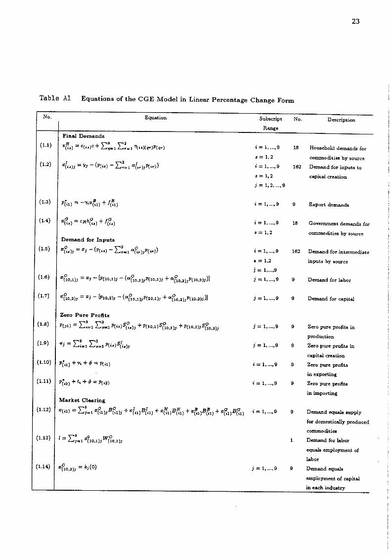
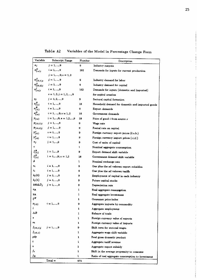
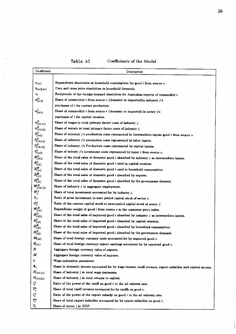
percentage change form are listed in Table A1 in the Appendix. The variables are definedin Table A2 and coefficients are described in Table A3. As can be seen from Table A1,the equations of the model are grouped under six headings.5

Final Demands

Final demands are divided into four categories: household consumption, investment,exports and government demand. Consumers are assumed to maximise a nested utilityfunction subject to an aggregate budget constraint. At the first level, we use the Leontieffunction implying no substitution between effective units of commodities. The effectiveunits of commodities are the Cobb-Douglas aggregation of imported and domestic goodsbelonging to the same commodity group. Thus at this second level, consumers have thesubstitution possibilities between domestic and imported commodities of the same typeaccording to a Cobb-Douglas function. The resultant set of household demand functions

for domestic and imported commodities are given by equation (1.1) in Table A1.

It is assumed that each industry uses sector specific capital goods. These capital units foruse in a given sector are created in a perfectly competitive environment under constantreturns to scale two-tiered production technology. At the first level, industry j chooseseffective intermediate inputs to minimise the total cost of capital creation subject to aLeontief production function. At the second level, industry j chooses its inputs for capitalcreation from domestic and imported sources to minimise costs subject to a Cobb-Douglas production function. The input demand functions derived from this specificationare given by equation (1.2) in Table A1.

In relation to exports, each commodity faces less than perfectly elastic demand curveThe relevant export demand functions of the model are represented by equation (1.3). Theelasticity of export demand facing producers vary across industries. Government demand

4 See Dixon et al. (1982, ch.3)for details.5 More details regarding the theory and the derivation of the equation system of themodel are available in Siriwardana (1994).

7

for domestic and imported commodities is explicitly recognised though the modelcontains no particular theory to describe the government behaviour. These demandfunctions appear as equation (1.4).

Industry Demands for Inputs

Producers of current goods are assumed to minimise the production costs subject to two-

level nested production function. The first level contains the constant returns to scaleLeontief production technology. This technology implies no substitution betweendifferent types of intermediate inputs and between intermediate inputs and primaryfactors. At the second level, producers substitute between domestically producedintermediate inputs and imports, and between different types of primary factors accordingto a Cobb-Douglas technology. The cost minimisation subject to this production

technology gives demand functions for intermediate inputs and for primary factors (seeequations (1.5), (1.6) and (1.7) in Table A1).

Zero Pure Profits

The assumption of constant returns to scale in production and competitive pricingbehaviour in each of the economic activity ensure that zero pure profits are earned inequilibrium. Equations (1.8), (1.9), (1.10) and (1.11) in Table A1 impose these zero profitconditions for production, capital creation, exporting and importing respectively.

Market clearing

Equations (1.12), (1.13), and (1.14) indicate that supply equals demand for domestically

produced commodities, labour and fixed capital respectively. However, it is important tonotice that the latter two equations do not necessarily imply full employment conditionsfor factors.

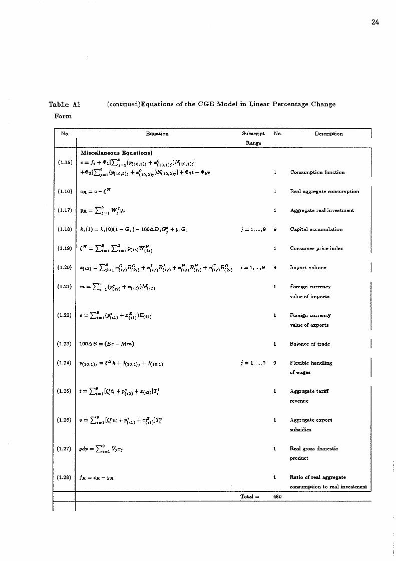
Miscellaneous Equations

Most of the equations listed under this heading are self-explanatory. Equation (1.15)represents the consumption function of the model. The characteristics of a Keynesiantype consumption function are embodied in this equation. Equation (1.16) gives realaggregate consumption and equation (1.17) defines the aggregate real investment. Thecapital accumulation of the economy is described by equation (1.18). It implies that thevariables which influence the capital stock at the end of one period are the current capitalstock, the depreciation rate and the current level of investment. The consumer price index

8

of the model is given by equation (1.19). Import volumes in domestic currency terms aredescribed by equation (1.20). Equations (1.21) and (1.22) give total import bill and exportrevenue in terms of foreign currency respectively. The balance of trade for the Australianeconomy is defined by equation (1.23). Equation (1.24) provides a flexible way ofhandling wages by indexing money wages to the consumer price index. Equations (1.25)and (1.26) define the aggregate tariff revenue and export subsidies respectively. Equation(1.27) is included in the model to project the changes in real gross domestic product(GDP). Finally, equation (1.28) defines the ratio of real aggregate consumption to realaggregate investment.

IV Calibration of the Model

The calibration process of the model involves the assignment of numerical values for a

large number of parameters. Our approach to parameterize the model is typical of thatgenerally adopted in applied general equilibrium analysis. The data required includevarious shares or weights (e.g., sales and cost shares) and estimates of the elasticityparameters such as household demand elasticities, capital-labour substitution elasticitiesand export demand elasticities. In choosing the values for parameters, a reference is madeto the existing econometric studies so as to be consistent with a given historicalbenchmark data set. The use of Leontief and Cobb-Douglas functional forms in thepresent model allows almost all the parameters to be derived from input-output tables.6

For the present model a benchmark database was compiled for the Australian economyfor the year 1934/35.7

The export demand elasticities which are required to implement the export demandfunctions of the model are not available for Australia for the time period underconsideration. Thus, plausible values for export demand elasticities were determined byreference to an econometric study for the United Kingdom and the United States (1921-1938) by Zelder (1958). The values for export demand elasticities chosen for thesimulations of the model are 2.0 for agriculture, pastoral and mining and 20.0 for other

sectors.

6 Detailed technical discussions concerning the computational procedure of theseparameters and coefficients from input-output tables can be found in Dixon et al. (1982,ch.2) and Higgs (1987, pp.41-56).7 M.F. Rola provided an excellent research assistance in compiling this inpu-output database. Full details of the data tables are available from the author upon request. See alsoSiriwardana (1987) for details on the construction of historical input-output tables.

9

V Economic Environment of the Simulations

The model described in the previous sections could be used to explore the implications ofvarious policies implemented and proposed during the depression. We have chosen thefollowing four policies to analyse using the model: (1) the increase in tariffs, (2) thereduction in government expenditure, (3) the devaluation of the Australian currency and(4) the reduction in real wages. Experiments (1) to (3) reflect the major policy changesthat were supposed to have contributed to the recovery. To evaluate the impact of thesepolicies we impose exogenously on the model a 30 per cent increase in all tariffs, a 20 percent reduction in government current expenditure and a 30 per cent devaluation of theAustralian pound. Experiment (4) dealing with the reduction of real wages is concernedwith the decision by the Arbitration Court in January 1931 to cut real wages by 10 percent.8

Some of the features of the macroeconomy are not projected endogenously by the model.Therefore, having decided the exogenous shocks to be imposed, we should specify themacroeconomic environment under which the proposed simulations would be carried out.The CGE model as described earlier contains 573 variables and 480 equations (see TablesA1 and A2). Thus, the number of variables exceeds the number equations by 93. Toobtain a solution for the model, this number of variables must be declared exogenous.Table A4 in the Appendix contains the chosen list of exogenous variables for the aboveexperiments. The selection of exogenous variables and assignment of values for them andfor the wage indexation parameter of the model create the economic environment for thesimulations.9

The model is simulated to examine the impact of various policies under a number ofalternative sets of assumptions concerning the macroeconomic environment. The

particular assumptions underlying the simulations are as follows: (1) industry-specificfixed capital in use are exogenous; (2) the real wages are constant; (3) real privateconsumption varies with real disposable income; (4) the shares of real privateconsumption, real government consumption and real investment in total real domesticabsorption remain unchanged; and (5) the nominal exchange rate is exogenous.Assumption (1) implies that the analysis is concerned with the short-run effects of the

8 It is apparent that many employers could not implement the wage cut as proposed dueto the labour unrest. Therefore it is doubtful whether the wage policy has produced its fullimpact towards the recovery.9 The computation of the solution for the present model was performed by using the(4.2.02) version of GEMPACK. This allows the use of multi-step solution approachwhich minimizes the Johansen linearization errors of the model. See Codsi and Pearson(1988) for details on GEMPACK.

10

policies considered. Assumption (2) indicates a slack labour market for the Australianeconomy and this is appropriate for the depression period. Assumptions (3) and (4) implythat the real domestic absorption is endogenously determined in all simulations. Finally,assumption (5) sets the numeraire of the model. Thus, all domestic price changes aremeasured relative to the world prices.

VI Simulation Results

Tables 1 and 2 report the projected effects of the four policy simulations on a number ofmacroeconomic and industry variables. The results are typically presented in percentagechange form so that they can be interpreted as elasticities. Furthermore, the simultaneousimpact of the four policies on a given endogenous variable can be obtained by summingacross the four columns in Tables 1 and 2. The findings of course depend on the modelassumptions and the economic environment under which the policies were simulated. Wediscuss below the macroeconomic and sectoral impact of each of the four policies.

(i) The Effects of the Increase in Tariffs

The tariff increase was one of the important policies adopted in the early 1930s to aid therecovery in Australia.10 The projections reported in column I of Table 1 indicate thelikely impact of the across-the-board increase in protection by 30 per cent on the mainmacroeconomic variables. Overall, these results tend to suggest that the tariff increaseswere relatively unimportant at macro level in the recovery process. The negligibleimprovement in aggregate employment (a 0.07 per cent) of the economy reflects the factthat the protection has had a little impact on recovering the lost ground in employment. It

appears that the increased employment in the import-competitive manufacturing sector islargely offset by the decline of employment in export sectors of the economy. The tariff

increase improves the competitive position against imports of the import-competitiveindustries, resulting employment and output gains in those industries. However, this

induces a rise in the economy’s domestic cost structure particularly with the full wageindexation, thus worsening the competitiveness of exporting sectors. These sectorsheavily rely on world markets and are unable to pass on the cost increases in the form ofhigher selling prices. As a result, the primary goods producing exporting sectorsexperience a decline in outputs and employment.

10 Australia is one of the countries which has very long history of protective tariffpoliciies. The origins of protection as an integral part of the industrial policy goes as farback as 1850s with the aftermath of the gold rush during the colonial period. For detailssee Siriwardana (1991).

11

Table I Projected Macroeconomic Effects of Various Policies(a)

Variable 30% increase 20% cut in 30% 10% reductionin tariffs government devaluation in real wages

expenditure(I) (II) ~II) (IV)

Real GDP 0.04 - 1.20 5.09 8.94

Real Income 1.33 - 1.56 4.55 8.22

Terms of trade 8.26 - 1.78 -2.10 -5.06

Real domesticabsorption

Aggregateexports(b)

Aggregateimports(b)

Balanceof trade

Consumer priceindex

Aggregatedemandfor labour(c)

2.79 -2.47 4.43 7.58

-8.26 1.78 2.31 5.06

0.83 -5.71 0.09 -2.52

-1.36 1.01 0.34 1.09

28.92 -6.22 20.84 -16.97

0.07 -2.12 9.17 15.76

Money wages 28.92 -6.22 14.64 -26.97

Real wages(d) 0.00 0.00 -6.20 -10.00

Nominalexchange rate

Real exchangerate(e)

0.00 0.00 30.00 0.00

-28.92 6.22 9.16 16.97

Notes: (a) All projections are in percentage changes except the balance of trade which is expressed asa percentage of base period GDP.(b) These are in foreign currency terms.(c) This projection shows the effective demand for labour.(d) Calculated by deflating movements in money wages by movements in the model’sconsumer price index.(e) Calculated by subtracting the percentage change in the model’s consumer price index fromthe percentage change in the nominal exchange rate.

12

It is interesting to note that the 30 per cent across-the-board increase in tariffs raises thereal income by 1.3 per cent and the real domestic absorption by 2.7 per cent. Theimprovement in domestic consumption induces demand for imports by 0.8 per centdespite the increased protection. This finding leads to some scepticism over theimportance of the protectionist policy to the recovery process by switching from imports

to domestic production. As Thomas (1988) pointed out, it appears that the growth indomestic demand has served as the main driving force of the manufacturing recoveryrather than the process of substitution of domestic production for imports. The resultsshow an 8.2 per cent decline in exports leading to a balance of trade deficit which isequivalent to a 1.3 per cent decrease in GDP in the base period.

The sectoral results which appear in column I of Table 2 help further to explain themacroeconomic picture of the economy under increased protection levels. They reveal

that the three export sectors (i.e., agriculture, pastoral and mining) are the losers from thepolicy of protection. The output and employment contraction in these three sectors isexplained by the cost-price squeeze imposed on primary producers by the inflationaryeffects of tariffs. It is clear that the manufacturing sector together with the rest of theeconomy benefited from increased protection at the expense of the exporting sectors.

(ii) The Effects of the Reduced Government Expenditure

The reduction of government current expenditure was an important aspect of thePremier’s plan. One of the objectives behind this policy was to create savings within thegovernment in order to make repayments of Australia’s overseas debts. The deflationaryimpact of the contraction was supposed to improve the competitiveness which woodboost exports, helping balance of payments. Column II of Table 1 shows themacroeconomic impact of the slashing government expenditure by 20 per cent. The moststriking result is the 2.1 per cent decline in the aggregate demand for labour in response

to this contractionary fiscal policy. Corresponding with this, there is a 1.2 per cent declinein the real GDP. The improvement in the competitiveness stemmed from the deflationaryimpact has produced an increase in exports by 1.7 per cent. The real domestic absorptiondeclines by 2.4 per cent. This in turn reduces the demand for imports by 5.7 per cent.These movements in exports and imports have created a very moderate surplus (i.e. 1 percent of the base period GDP) in the balance of trade. Though this is helpful in an attemptto overcome balance of payment difficulties, it appears to have cost considerable amountof employment opportunities in the economy. When weighed against the employmentloss, the contrationary fiscal policy does not appear to have been that attractive in therecovery process from the depression.

13

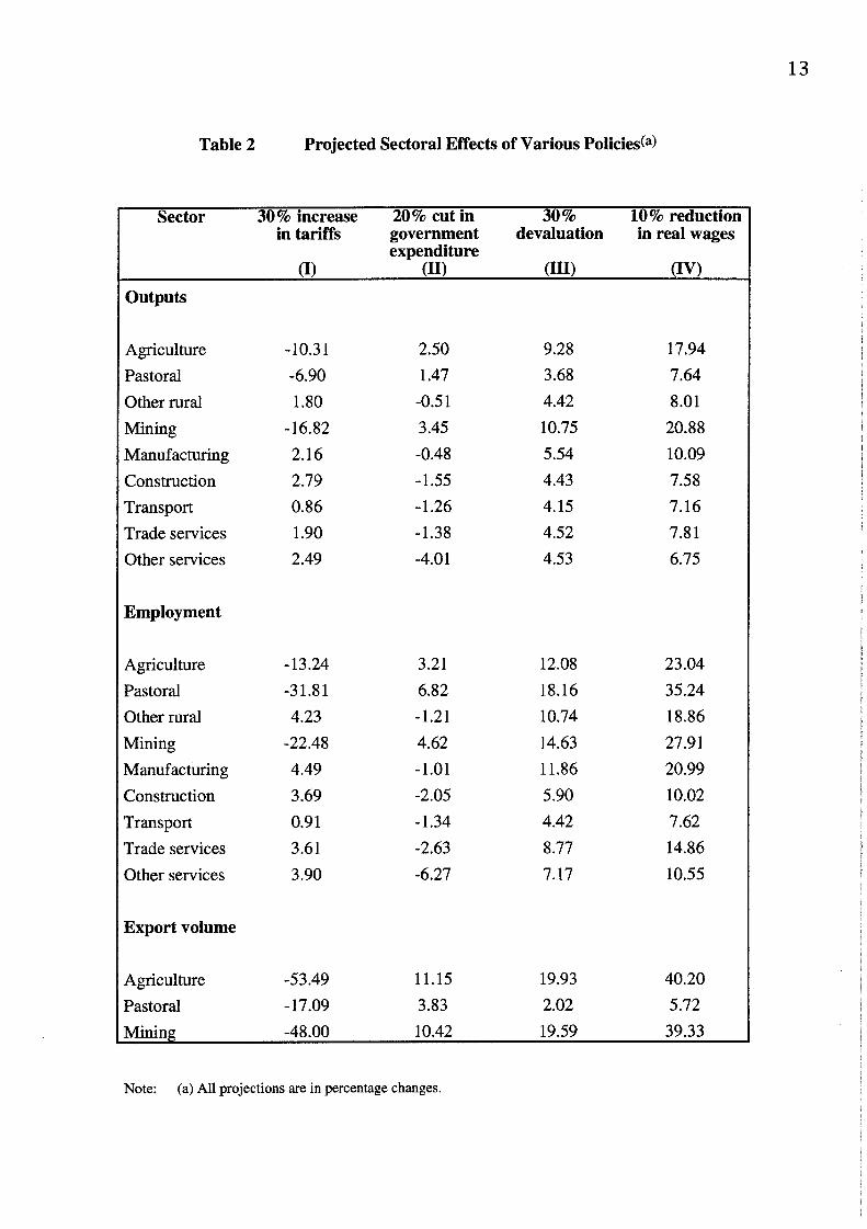
Table 2 Projected Sectoral Effects of Various Policies(a)

Sector

Outputs

30% increase 20% cut in 30% 10% reductionin tariffs government devaluation in real wages

expenditure(I) (II) (III) (~)

Agriculture - 10.31 2.50 9.28 17.94

Pastoral -6.90 1.47 3.68 7.64

Other rural 1.80 -0.51 4.42 8.01

Mining - 16.82 3.45 10.75 20.88

Manufacturing 2.16 -0.48 5.54 10.09

Construction 2.79 - 1.55 4.43 7.58

Transport 0.86 -1.26 4.15 7.16

Trade services 1.90 - 1.38 4.52 7.81

Other services 2.49 -4.01 4.53 6.75

Employment

Agriculture - 13.24 3.21 12,08 23.04Pastoral -31.81 6.82 18.16 35.24Other rural 4.23 - 1.21 10.74 18.86Mining -22.48 4.62 14.63 27.91Manufacturing 4.49 - 1.01 11.86 20.99Construction 3.69 -2.05 5.90 10.02Transport 0.91 - 1.34 4.42 7.62

Trade services 3.61 -2.63 8.77 14.86

Other services 3.90 -6.27 7.17 10.55

Export volume

Agriculture -53.49 11.15 19.93 40.20

Pastoral -17.09 3.83 2.02 5.72

Minin~ -48.00 10.42 19.59 39.33

Note: (a) All projections are in percentage changes.

14

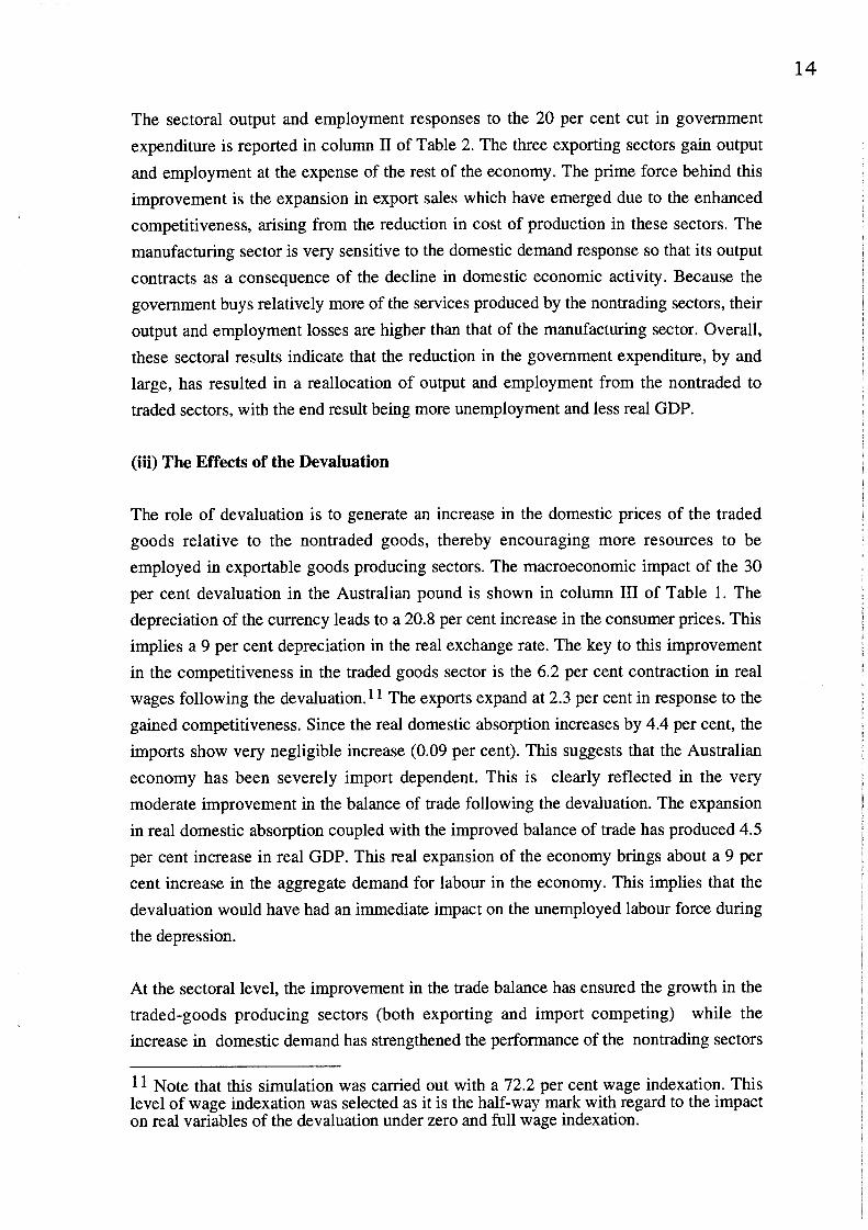
The sectoral output and employment responses to the 20 per cent cut in governmentexpenditure is reported in column II of Table 2. The three exporting sectors gain output

and employment at the expense of the rest of the economy. The prime force behind thisimprovement is the expansion in export sales which have emerged due to the enhancedcompetitiveness, arising from the reduction in cost of production in these sectors. Themanufacturing sector is very sensitive to the domestic demand response so that its outputcontracts as a consequence of the decline in domestic economic activity. Because thegovernment buys relatively more of the services produced by the nontrading sectors, theiroutput and employment losses are higher than that of the manufacturing sector. Overall,these sectoral results indicate that the reduction in the government expenditure, by andlarge, has resulted in a reallocation of output and employment from the nontraded totraded sectors, with the end result being more unemployment and less real GDP.

(iii) The Effects of the Devaluation

The role of devaluation is to generate an increase in the domestic prices of the tradedgoods relative to the nontraded goods, thereby encouraging more resources to beemployed in exportable goods producing sectors. The macroeconomic impact of the 30per cent devaluation in the Australian pound is shown in column III of Table 1. Thedepreciation of the currency leads to a 20.8 per cent increase in the consumer prices. Thisimplies a 9 per cent depreciation in the real exchange rate. The key to this improvementin the competitiveness in the traded goods sector is the 6.2 per cent contraction in realwages following the devaluation. 11 The exports expand at 2.3 per cent in response to thegained competitiveness. Since the real domestic absorption increases by 4.4 per cent, theimports show very negligible increase (0.09 per cent). This suggests that the Australianeconomy has been severely import dependent. This is clearly reflected in the very

moderate improvement in the balance of trade following the devaluation. The expansionin real domestic absorption coupled with the improved balance of trade has produced 4.5

per cent increase in real GDP. This real expansion of the economy brings about a 9 percent increase in the aggregate demand for labour in the economy. This implies that thedevaluation would have had an immediate impact on the unemployed labour force duringthe depression.

At the sectoral level, the improvement in the trade balance has ensured the growth in thetraded-goods producing sectors (both exporting and import competing) while theincrease in domestic demand has strengthened the performance of the nontrading sectors

11 Note that this simulation was carried out with a 72.2 per cent wage indexation. Thislevel of wage indexation was selected as it is the half-way mark with regard to the impacton real variables of the devaluation under zero and full wage indexation.

15

of the economy. As can be seen from the sectoral output and employment projections, thedevaluation has favoured the export sectors as usual. The largest output gains areprojected for mining and agriculture followed by manufacturing. However, thedevaluation has also provided an even stimulation to the nontrading sectors which haveexperienced output growth in line with that of the economy as a whole.

(iv) The Effects of the Reduction in Real Wages

The results indicate that reduction in real wages would have had a very significant impactover the economy. Our findings are somewhat surprising, given the different viewsconcerning the implementation of the 10 per cent real wage cut proposed by theArbitration Commission in early 1931. The macroeconomic results of the simulationreported in column IV of Table 1 indicate that the wage reduction has been the mostattractive policy. An increase in aggregate employment of 15.7 per cent is projectedfollowing the 10 per cent cut in real wages. This does imply that the employmentrecovery during the depression was heavily dependent on the wage flexibility downward.This employment gain in turn produces 8.9 per cent expansion in real GDP. Since there isa deterioration in the terms of trade, the real income increases slightly less than this (i.e.8.2 per cent). This overall expansion in the economy results in a 7.5 per centimprovement in the real domestic absorption.

It is further evident from the results that the 10 per cent wage cut has generated a 17 percent reduction in the consumer price index. The implied cost reduction in the domesticeconomy stemmed from this deflationary impact has improved the competitiveness ofexports and import-competing sectors of the economy. This is clearly shown by the 17per cent depreciation of the real exchange rate. Consequently, aggregate exports increase

by 5 per cent and aggregate imports decline by 2.5 per cent, creating a positive tradebalance which is equivalent to 1 per cent of real GDP.

The sectoral level projections reported in Table 2 (see column IV) indicate clearly theadvantage of the reduced wage costs and the resulting adjustments at industry level. Themajor beneficiaries of the wage cut are the trading sectors of the economy. Among these,agriculture, mining, pastoral and manufacturing sectors experience very significant outputand employment gains. They in turn reflect their improvement in competitiveness. Theexpansion in the former three sectors are mainly explained by the increased export salesfollowing the reduction in costs stemmed from the wage decline. The manufacturingsector has benefited from the domestic demand expansion. The nontrading sectors of theeconomy also follow the same trend, reflecting output and employment gains in line with

the overall performance of the economy.

16

An Alternative Policy Mix

The simulation results presented in the previous section indicate the economic impact ofvarious policies adopted during the depression. A glance at these results confirm that realwages and the devaluation have been the key to economic recovery. The diverging resultsof these policies also imply that there would have been alternative policies or mix ofpolicies that would have produced more successful outcome. In this section we consider

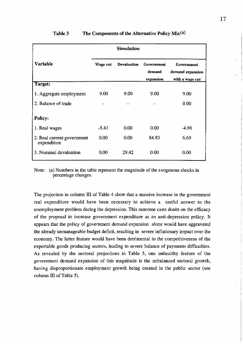
four such policy prescriptions. In order to facilitate the comparison, the four simulationsare calibrated so that each option results in a 9 per cent increase in aggregateemployment. The employment growth of this magnitude was expected to be sufficient toreach the pre-depression level of economic stability. Table 3 contains a summary of thepolicy mix simulated under this scenario. According to our model, it is apparent that thetarget of 9 per cent increase in employment could be achieved by any of the followingalternatives: (1) a 5.41 per cent real wage cut; or (2) a 29.42 per cent nominaldevaluation; or (3) a 84.83 per cent increase in real current government expenditure; or(4) a 6.69 per cent increase in real current government expenditure combined with 4.98per cent real wage cut. As Table 3 reveals, the latter simulation is intended to achieve twotargets; the 9 per cent employment growth while having zero impact on the balance oftrade.

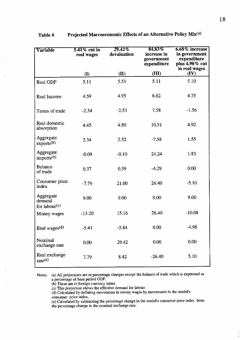
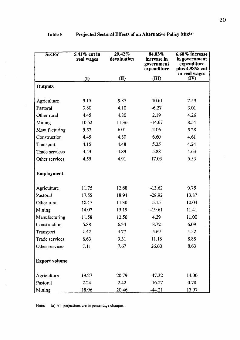
Tables 4 and 5 contains the projected impact of this alternative policy mix onmacroeconomic and sectoral variables respectively. Column I of Table 4 suggests that theemployment recovery through a real wage cut which is substantially less than thatproposed by the Arbitration Commission would have been a feasible option. A wagereduction of this magnitude could have improved the competitiveness in the traded goodssector significantly. The sectoral output and employment projections reported in Table 5show that the real wage cut would have favoured the traded good sector.

Our projections also point out that the success of the nominal devaluation in achieving

the employment target was conditioned by a reduction in real wages. Though theinflationary impact of the devaluation was an unavoidable outcome, such policy wouldhave provided a useful solution to the balance of payments problem during thedepression. The substantial growth in traded sectors of the economy supports this

observation.

17

Table 3 The Components of the Alternative Policy Mix(a)

Simulation

Variable Wage cut Devaluation Government Government

demand demand expansion

expansion with a wage cutTarget:

1. Aggregate employment 9.00 9.00 9.00 9.00

2. Balance of trade - - 0.00

Policy:

1. Real wages -5.41 0.00 0.00 -4.98

2. Real current government 0.00 0.00 84.83 6.69expenditure

3. Nominal devaluation 0.00 29.42 0.00 0.00

Note: (a) Numbers in the table represent the magnitude of the exogenous shocks inpercentage changes.

The projection in column III of Table 4 show that a massive increase in the government

real expenditure would have been necessary to achieve a useful answer to theunemployment problem during the depression. This outcome casts doubt on the efficacyof the proposal to increase government expenditure as an anti-depression policy. Itappears that the policy of government demand expansion alone would have aggravatedthe already unmanageable budget deficit, resulting in severe inflationary impact over theeconomy. The latter feature would have been detrimental to the competitiveness of theexportable goods producing sectors, leading to severe balance of payments difficulties.As revealed by the sectoral projections in Table 5, one unhealthy feature of thegovernment demand expansion of this magnitude is the unbalanced sectoral growth,having disproportionate employment growth being created in the public sector (seecolumn HI of Table 5).

18

Table 4 Projected Macroeconomic Effects of an Alternative Policy Mix(a)

Variable

Real GDP

5.41% cut in 29.42% 84.83%real wages devaluation increase in

governmentexpenditure

(I) (II) (III)

5.11 5.51 5.11

6.68% increasein government

expenditureplus 4.98% cutin real wages

(iv)5.10

Real Income 4.59 4.95 6.62 4.75

Terms of trade -2.34 -2.53 7.58 - 1.56

Real domesticabsorption

Aggregateexports(b)

Aggregateimports(b)

Balanceof trade

Consumer priceindex

Aggregatedemandfor labour(c)

4.45 4.80 10.51 4.92

2.34 2.52 -7.58 1.55

-0.09 -0.10 24.24 1.83

0.37 0.39 -4.29 0.00

-7.79 21.00 26.40 -5.10

9.00 9.00 9.00 9.00

Money wages - 13.20 15.16 26.40 - 10.08

Real wages(d) -5.41 -5.84 0.00 -4.98

Nominal 0.00 29.42 0.00 0.00exchange rate

Real exchange 7.79 8.42 -26.40 5.10rate(e)

Notes: (a) All projections are in percentage changes except the balance of trade which is expressed asa percentage of base period GDP.(b) These are in foreign currency terms.(c) This projection shows the effective demand for labour.(d) Calculated by deflating movements in money wages by movements in the model’sconsumer price index.(e) Calculated by subtracting the percentage change in the model’s consumer price index fromthe percentage change in the nominal exchange rate.

19

The results in column IV of Table 4 imply that an increase in real governmentexpenditure combined with a reduction in real wages, while having zero impact on thebalance of trade, would have been an attractive policy package. It seemed to have hadenough strength to turn around the effects of the isolated public demand expansionpolicy. The other attractive feature of this package is that it involves with a smaller wagecut and a smaller increase in government expenditure. The sectoral results presented inTable 5 suggest that such government demand expansion coupled with a wagemoderation would have generated balanced stimulation of the economy, creating moreevenly distributed employment growth between public and private sectors.

VII Conclusion

The simulation results presented in this paper proved the fact that the CGE model is auseful tool for the analysis of the impact of various policies during the depression. Whilethis approach is widely used at present for economic policy analysis, it is still novel tostudies in historical context. Of the four policies examined in this paper, the nominaldevaluation and the real wage reduction appeared to have contributed to the relativelyspeedy recovery from the 1930s depression in Australia. The wage flexibility downwardwould have been a crucial factor to success of the recovery process. In contrast to thewidely held conventional view, the increased tariff protection in the early 1930s is likelyto have contributed very little towards the employment recovery. It is also apparent fromthe present analysis that the contrationary fiscal policy such as the reduction ingovernment expenditure would have cost substantial job opportunities though it wouldhave had some favourable impact on the balance of payments.

Our analysis of the alternative policy-mix brings into light many implications for policiesproposed in different plans canvassed in this period. It is clear that the implementation ofthe Theodore’s Plan which was fundamentally based on the expansion of the publicexpenditure would have created massive budgetary problems with severe adverse impacton the balance of payments. It is likely that the extra expenditure resulting from suchexpansion in the government sector would be absorbed partly by imports and partly bynontradables. This familiar Keynesian type employment creation program would haveundoubtedly deteriorated the balance of trade and would have retarded the growth of theprimary goods producing exporting sectors which were fundamental to the Australianrecovery.

20

Table 5 Projected Sectoral Effects of an Alternative Policy Mix(a)

Sector

Outputs

5.41% cut in 29.42%real wages devaluation

84.83% 6.68% increaseincrease in in governmentgovernment expenditureexpenditure plus 4.98% cut

in real wagesfin) or)(I) (II)

Agriculture 9.15 9.87 - 10.61 7.59

Pastoral 3.80 4.10 -6.27 3.01

Other rural 4.45 4.80 2.19 4.26

Mining 10.53 11.36 - 14.67 8.54

Manufacturing 5.57 6.01 2.06 5.28

Construction 4.45 4.80 6.60 4.61

Transport 4.15 4.48 5.35 4.24

Trade services 4.53 4.89 5.88 4.63

Other services 4.55 4.91 17.03 5.53

Employment

Agriculture 11.75 12.68 - 13.62 9.75

Pastoral 17.55 18.94 -28.92 13.87

Other rural 10.47 11.30 5.15 10.04

Mining 14.07 15.19 - 19.61 11.41

Manufacturing 11.58 12.50 4.29 11.00

Construction 5.88 6.34 8.72 6.09

Transport 4.42 4.77 5.69 4.52

Trade services 8.63 9.31 11.18 8.88

Other services 7.11 7.67 26.60 8.63

Export volume

Agriculture 19.27

Pastoral 2.24

Minin 18.96

20.79 -47.32 14.00

2.42 -16.27 0.78

20.46 -44.21 13.97

Note: (a) All projections are in percentage changes.

21

The paper illustrates that the 10 per cent real wage cut proposed by the ArbitrationCommission was more than what was required to achieve the employment goal. Oursimulation results imply that little more than half of the proposed reduction (i.e., 5.4 per

cent) would have been sufficient to create the employment opportunities for unemployedby reducing inflation and improving the international competitiveness of the economy.Another interesting finding from the alternative policy-mix is the likely combined impactof the government demand expansion with a real wage moderation. This Keynesian-neoclassical policy package would have required only 6.68 per cent increase ingovernment expenditure and 4.98 per cent real wage cut to create the necessaryemployment growth. Of course this employment creation is under the assumption thatthe expansion in government expenditure and the real wage cut do not affect the balanceof trade. All in all, the present analysis implies that the reduction in real wages combined

with a moderate expansion in the domestic demand would have been the best policyprescription for Australia to reach the non-inflationary recovery from the depression inthe 1930s.

References

Boehm, E.A. (1973), "Australia’s Economic Depression of the 1930s", Economic Record,49, pp. 606-623.

Copland, D. (1934), Australia in the World Crisis 1929-1933. Cambridge : CambridgeUniversity Press.

Codsi, G. and Pearson, K.R. (1988), "GEMPACK: General Purpose Software for AppliedGeneral Equilibrium and Other Economic Modellers", Computer Science inEconomics and Management, 1, pp. 189-207.

Davidson, B.R. (1988), "Agriculture and Recovery from the Depression", In R.G.Gregory and N.G. Butlin (Eds.), Recovery from the Depression. New York:Cambridge University Press. pp. 273-288.

Dixon,P.B., Parmenter, B.R., Sutton, J. and Vincent, D.P. (1982), ORANI: AMultisectoral Model of the Australian Economy. Amsterdam: North-Holland.

DysterB. and Meredith, D. (1990), Australia in the International Economy. New York :Cambridge University Press.

Gregory, R.G. and Butlin, N.G. (Eds.) (1988), Recovery From the Depression. NewYork : Cambridge University Press.

Higgs,P.J. (1987), "MO87: A Three-Sector Miniature ORANI Model", ImpactPreliminary Working Paper, OP-63, Impact Project, University of Melbourne.

Johansen, L. (1974), A Multi-Sectoral Study of Economic Growth (2nd ed.). Amsterdam:North-Holland.

Schedvin, C.B. (1970), Australia and the Great Depression. Sydney : Sydney UniversityPress.

22

Siriwardana, A.M. (1985), "The Use of Computable General Equilibrium Models forHistorical Counterfactual Analysis", Working Papers in Economic History, no.38,Australian National University.

Siriwardana, A.M. (1987), "An Input Output Table for the Colony of Victoria in 1880",Australian Economic History Review, 27, pp.61-85.

Siriwardana, A.M. (1991), "The Impact of Tariff Protection in the Colony of Victoria inthe Late Nineteenth Century : A General Equilibrium Analysis", AustralianEconomic History Review, 31, pp.45-65.

Siriwardana, A.M. (1994), "The Causes of the Depression in Australia in the 1930s : AGeneral Equilibrium Evaluation", forthcoming in Explorations in EconomicHistory.

Spenceley, G. (1990), A Bad Smash. Melbourne: Penguin Books Australia.

Thomas, M. (1988), "Manufacturing and Economic Recovery in Australia, 1932-1937",In R.G. Gregory and N.G. Butlin (Eds.), Recovery From the Depression. NewYork : Cambridge University Press. pp. 246-272.

Valentine, T. (1987), "The Causes of the Depression in Australia", Explorations inEconomic History, 24, pp. 43-62.

Valentine, T. (1988), "The Battle of the Plans : A Macroeconometric Model of theInterwar Economy", In R.G. Gregory and N.G. Buflin (Eds.), Recovery From theDepression. New York : Cambridge University Press.

Zelder,R.E. (1958), "Estimates of Elasticities of Demand for Exports of the UnitedKingdom and the United States, 1921-1938", The Manchester School of Economicand Social Sciences, 26, pp.33-47.

23

Table A1 Equations of the CGE Model in Linear Percentage Change Form

(1.4)

(1.s)

(i.z)

11.9)

’,1.10)

:1.11)

11.12)

1.13)

1.14)

No. Subscript No. Description

Range

18

Equation

Final Demands

~ : 1 ..... 9 Household demands for

s = 1, 2 commodities by source

~ = 1 ..... 9 162 Demand for inputs to

s = 1, 2 capital creation

j = I, 2 ..... 9

~ = 1,...,9 9 Export demands

Demand for Inputs

18 Government demands for

commodities by source

1, ..., 9 162 Demand for intermediate

1,2 inputs by source

1...9

1 .....9 9 Demand for labor

~o,~)# = =# - [P~o,~)~ - ( (~0,~)#P(~0,~)~ + =~0,~)#~(~0,~)~)] 3" = 1,...,9 9 Demand for capital

Zero Pure Profits

: E~=I " 0

~(,.,)S~i=).~ o

~i~) + ~ + � =

Market Clearing

_ ~ ~o ~o ~ zl BI ~ zH mH ~ ~ m~ ~ ~O BGz(~)- ~#=~ (~)~(~,)#. (~) (~z)~ (i~)~(i,)~ (~,)~(~)~ (~,) (~)

~#=~ (~o,~)# (~o.~)~

=o = ,~#(o)(zo,2).~

j = 1, ...,9

~ = 1, .... 9

’/= 1, ...,9

Zero pure profits in

production

Zero pure profits in

capital creation

Zero pure profits

in exporting

Zero pure profits

in importing

Demand equals supply

for domesticaUy produced

commodities

Demand for labor

equals employment of

labor

Demand equah

employment of capital

in each industry

24

Table A1

Form

(continued)Equations of the CGE Model in Linear Percentage Change

No. Equation Subscript No. Description

Range

(1.15)

(1.16)

(1.1~’)

0.19)

(1.2o)

(1.21)

(1.22)

(1.23)

(1.24)

(1.25)

(~m’)

Miscellaneous Equations)

9

+ ~[~-~=~(~(~0,~)~ +~0 Consumption ~unction

Real aggregate consumption

1 Aggregate real investment

i = 1, ...9

9 Capital accumulation

1 Consm~er price index

9 Import volume

1 Foreign currency

value of imports

Foreign curremcy

value of exports

IOOAB = (Ee - Mm) 1 BMance of trade

P(~0,1)# = ~sh +/(~0,i)# + J(~0,1) 3’ = 1, ...,9 9 Flexible handling

of wages

9 t Aggregate tariff

reveDlle

Aggregate export

subsidies

Real ~ross domestic

product

Total =

I Ratio of real aggregate

consumption to real investment

48O

25

Table A2 Variables of the Model in Percentage Change Form

Variable

~o(~)~

Subscript P~nge

= 1 ....,9

~ = 1,...,9

= 1,...,9;s = 1,2

= 1 .....9

= 1 .....9

1,...,9

s= 1,2;3"=1,2, .... 9

= 1,2, ....9

1, -.9

1, ...,9

9;s = 1,2

1,...,9; s = 1,2,..,9

1, ...,9

1, ...,9

1, ...,9

1,...,9

1.-,9

i = 1,...,9

i = 1,...,9; s = 1,2

~ = 1, ...,9

~ = 1, ...,9

3" = 1, ...,9j = 1 .....9

3" = 1 ..... 9

.~ = 1 .... ,9

Tot~ =

Number

9

162

9

9

162

9

18

9

18

18

9

9

9

9

9

1

9

18

1

9

9

9

9

9

1

1

1

9

1

1

1

1

9

1

1

1

1

1

1

573

Description

Industry outputs

Demands for inputs for current production

Industry de~naud ~or labor

Industry demand ~or capital

Demands for inputs (domestic and imported)

~or capital creation

Sectoral capital formation

Household demand ~or domestic and imported goods

Export denmnds

Government demands

Price o~ good ~ ~rom source s

Wage rate

Rental rate on capital

Foreign currency export prices (~.o.b.)

Foreign currency import prices

Cost o~ units of capital

Nominal aggregate consumption

Export demand shift variable

Government demand shift variable

Nominal exchange rate

One plus the azl valorem export subsidies

One plus the ad valorem tariffs

Employment of capital in each industry

~’hture capital stocks

Depreciation rate

Real aggregate consun~tion

Real aggregate investment

Gomumer price index

Aggregate imports by commodity

Aggregate employment

Balance of trade

Foreign currency value o~ exports

Foreign currency value of imports

$~R term ~or sectoral wages

Aggregate wage shift variable

Real gross domestic product

Aggregate tarii~ revenue

Aggregate export subsidy

Shift in the average prope~ity to consume

Ratio of real aggregate consumption to investment

26

Table A3 Coefficients of the Model

Ooei~icient Description

e(~) Expenditure elasticities in household consumption for good ~ from source s.

~(~)(~) Own and cross price elasticities in household demands.

Reciprocals of the foreign demand elasticities for Australian exports of cormmodity

a~)~ Share of commodity ~ from source r (domestic or imported)in industry

purchases of ~ for current production.

c~rC~)#

Share of commodity ~ from source r (domestic or imported) in sector

purchases of ~ for capital creation.

~’~10,1).~ Share of wages in total primary factor costs of industry ~.

~,O(~o,~)~ Share of rentals in total primary factor costs of industry ~.

Share of industry j’s production costs represented by intermediate inputs good

~o,:)~ Sltare of industry ~’s production costs represented by labor inputs.

~o,~)~ Share of industry j’s Production costs represented by capital inputs.

Share of industr j’s investment costs represented by input ~ from source s.

B~)~ Share of the total sales of domestic good ~ absorbed by industry j as intermediate inputs.

B~) Share of the total sales of domestic good ~ used in capital creation.

Share of the total sales of domestic good ~ used in household consumption,

Share of the total sales of domestic good ~ absorbed by exports.

Share of the total sales of domestic good ~ absorbed by the government demand.

~o,~)~ Share of industry ~ in a~regate employment.

Share of total investment accounted for by industry ~.

o~ Ratio of ~ross investment to next period capitM stock of sector ~.

o; Ratio of the current capital stock to next-period capital stock of sector ~.

Expenditure weight of good i from source s in the c~uraer price index.

Share of the total sales of imported good ~ absorbed by industry ~ as intermediate inputs.

B~) Share of the total sales of imported good ~ absorbed by capital creation,

Share of the total sales of imported good ~ absorbed by household consumption.

Share of the total sales of imported good ~ absorbed by the govenunent demand.

~(~) Slu~re of total forei~ currency costs accounted for by imported good ~.

z(~) Share of total foreig~t currency export earnings accounted for by exported good

E Aggregate foreign currency value of exports.

Aggregate forei~ currency value of imports.

Wage indexation parameter.

@~ Share in domestic income accounted for by wage income, tariff revenue, export subsidies and capitM income.

N(,o,,)# Share of industry j in total wage payments,

~(~o,~)~ Share of industry j in total returns to capitM.

Ratio of the power of the tariff on good ~ to the ad valorem rate.

Share of total tariff revenue accounted for by tari~ on good ~.

Ratio of the power of the export subsidy on good ~ to the ad valorem rate.

Share of total export subsidies accounted for by export subsidies on good

Share of sector j in GDP.

27

Table A4

V~’iable Subscript Range

The Selection of Exogenous Variables

Number Description

P(~2)

f~il)

9

1,2,4

3,5, .... 9

1,..., 9

1,..., 9

1,..., 9

1,2

1,2 ..... 9

1,2 ..... 9

1 ....,9

9

9

3

6

9

9

18

9

9

9

1

1

1

Foreign currency import prices (c.i.f.)

One plus the ad valorem taxi~s

One plus the export subsidy for the major export commodities

The export volumes for the minor export commodities

Export demand shift variables

Employment of capital in each industry

Shifts in government demands

Depredation rate

Cost of units of capitM

Shift term for sectors wages

Aggregate wage shift variable

Nominal exchange rate

ShiR in the average propensity to consume

Total = 93

UNE Working Papers in Economics

Baldry, J.C. and Dollery, B.E. 1992. Investment and Trade Sanctions against SouthAfrica in a Model of Apartheid.

Wallis, J.L. and Dollery, B.E. 1993. The Economics:of Economics: A Model ofResearch Discourse.

Schulze, D.L. 1993. Financial Integration and Financial Development: A ConceptualFramework.

Dollery, B.E. and Whitten, S. 1994. An Empirical Analysis of Tariff Endogeneity inAustralia, 1904-1978.

Schulze, D.L. and Yong, Jong-Say. 1994. Rational Expectations and Monetary Policyin Malaysia.

Pullen, J.M. and Smith, G.O. 1994. Major Douglas and the Banks.

Pullen, J.M. 1994. Toward a Mathematical Model of Malthus.

Dollery, B.E. and Jackson, C. 1994. A Note on Methological Parallels BetweenAccounting and Economics.

Anwar, S. and Shamsuddin, A.F.M. 1994. Effects of Terms of Trade Changes in aPublic Input Economy.