![arXiv:1209.3431v1 [stat.ML] 15 Sep 2012aarti/pubs/MKolar_BlockCS.pdf · 2012. 9. 18. · arXiv:1209.3431v1 [stat.ML] 15 Sep 2012 arXiv: 0000.0000 RECOVERING BLOCK-STRUCTURED ACTIVATIONS](https://static.fdocuments.us/doc/165x107/6050b7794a1b290e094e5ae7/arxiv12093431v1-statml-15-sep-aartipubsmkolarblockcspdf-2012-9-18.jpg)
Recovering Structured Signals in Noise: Comparison Lemmas and ...
210
Recovering Structured Signals in Noise: Comparison Lemmas and the Performance of Convex Relaxation Methods Babak Hassibi California Institute of Technology EUSIPCO, Nice, Cote d’Azur, France August 31, 2015 Babak Hassibi (Caltech) Comparison Lemmas Aug 31, 2015 1 / 65
Transcript of Recovering Structured Signals in Noise: Comparison Lemmas and ...
Recovering Structured Signals in Noise:Comparison Lemmas and the Performance of Convex
Relaxation Methods
Babak Hassibi
California Institute of Technology
EUSIPCO, Nice, Cote d’Azur, FranceAugust 31, 2015
Babak Hassibi (Caltech) Comparison Lemmas Aug 31, 2015 1 / 65

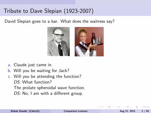
Tribute to Dave Slepian (1923-2007)
David Slepian goes to a bar. What does the waitress say?
a. Claude just came in.
b. Will you be waiting for Jack?
c. Will you be attending the function?DS: What function?The prolate spheroidal wave function.DS: No, I am with a different group.
d. Will you be joining the French table?
e. None of the above.
Babak Hassibi (Caltech) Comparison Lemmas Aug 31, 2015 2 / 65

Tribute to Dave Slepian (1923-2007)
David Slepian goes to a bar.
What does the waitress say?
a. Claude just came in.
b. Will you be waiting for Jack?
c. Will you be attending the function?DS: What function?The prolate spheroidal wave function.DS: No, I am with a different group.
d. Will you be joining the French table?
e. None of the above.
Babak Hassibi (Caltech) Comparison Lemmas Aug 31, 2015 2 / 65

Tribute to Dave Slepian (1923-2007)
David Slepian goes to a bar. What does the waitress say?
a. Claude just came in.
b. Will you be waiting for Jack?
c. Will you be attending the function?DS: What function?The prolate spheroidal wave function.DS: No, I am with a different group.
d. Will you be joining the French table?
e. None of the above.
Babak Hassibi (Caltech) Comparison Lemmas Aug 31, 2015 2 / 65

Tribute to Dave Slepian (1923-2007)
David Slepian goes to a bar. What does the waitress say?
a. Claude just came in.
b. Will you be waiting for Jack?
c. Will you be attending the function?
DS: What function?The prolate spheroidal wave function.DS: No, I am with a different group.
d. Will you be joining the French table?
e. None of the above.
Babak Hassibi (Caltech) Comparison Lemmas Aug 31, 2015 2 / 65

Tribute to Dave Slepian (1923-2007)
David Slepian goes to a bar. What does the waitress say?
a. Claude just came in.
b. Will you be waiting for Jack?
c. Will you be attending the function?DS: What function?
The prolate spheroidal wave function.DS: No, I am with a different group.
d. Will you be joining the French table?
e. None of the above.
Babak Hassibi (Caltech) Comparison Lemmas Aug 31, 2015 2 / 65

Tribute to Dave Slepian (1923-2007)
David Slepian goes to a bar. What does the waitress say?
a. Claude just came in.
b. Will you be waiting for Jack?
c. Will you be attending the function?DS: What function?The prolate spheroidal wave function.
DS: No, I am with a different group.
d. Will you be joining the French table?
e. None of the above.
Babak Hassibi (Caltech) Comparison Lemmas Aug 31, 2015 2 / 65
Tribute to Dave Slepian (1923-2007)
David Slepian goes to a bar. What does the waitress say?
a. Claude just came in.
b. Will you be waiting for Jack?
c. Will you be attending the function?DS: What function?The prolate spheroidal wave function.DS: No, I am with a different group.
d. Will you be joining the French table?
e. None of the above.
Babak Hassibi (Caltech) Comparison Lemmas Aug 31, 2015 2 / 65

Tribute to Dave Slepian (1923-2007)
David Slepian goes to a bar. What does the waitress say?
a. Claude just came in.
b. Will you be waiting for Jack?
c. Will you be attending the function?DS: What function?The prolate spheroidal wave function.DS: No, I am with a different group.
d. Will you be joining the French table?
e. None of the above.Babak Hassibi (Caltech) Comparison Lemmas Aug 31, 2015 2 / 65

Outline
IntroductionI structured signal recoveryI non-smooth convex optimizationI LASSO and generalized LASSO
Comparison LemmasI Slepian, Gordon
Squared Error of Generalized LASSOI Gaussian widths, statistical dimensionI optimal parameter tuning
GeneralizationsI other loss functionsI other random matrix ensembles
Summmary and Conclusion
Babak Hassibi (Caltech) Comparison Lemmas Aug 31, 2015 3 / 65
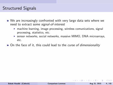
Structured Signals
We are increasingly confronted with very large data sets where weneed to extract some signal-of-interest
I machine learning, image processing, wireless comunications, signalprocessing, statistics, etc.
I sensor networks, social networks, massive MIMO, DNA microarrays,etc.
On the face of it, this could lead to the curse of dimensionality
Fortunately, in many applications, the signal of interest lives in amanifold of much lower dimension than that of the original ambientspace
In this setting, it is important to have signal recovery algorithms thatare computationally efficient and that need not access the entire datadirectly (hence compressed recovery)
Babak Hassibi (Caltech) Comparison Lemmas Aug 31, 2015 4 / 65

Non-Smooth Convex Optimization
Non-smooth convex optimization has emerged as a tractable methodto deal with such structured signal recovery methods
Given the observations, y ∈ Rm, we want to obtain some structuredsignal, x ∈ Rn
I a convex loss function L(x , y) (could be a log-likelihood function, e.g.)I a (non-smooth) convex structure-inducing regularizer f (x)
The generic problem is
minxL(x , y) + λf (x) or min
L(x ,y)≤c1
f (X ) or minf (x)≤c2
L(x , y)
Babak Hassibi (Caltech) Comparison Lemmas Aug 31, 2015 5 / 65

Non-Smooth Convex Optimization
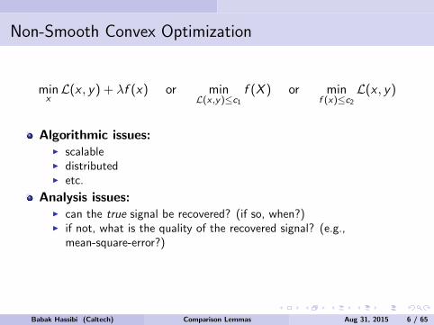
minxL(x , y) + λf (x) or min
L(x ,y)≤c1
f (X ) or minf (x)≤c2
L(x , y)
Algorithmic issues:I scalableI distributedI etc.
Analysis issues:I can the true signal be recovered? (if so, when?)I if not, what is the quality of the recovered signal? (e.g.,
mean-square-error?)I how does the convex approach compare to one with no computational
constraints?I how to choose the regularizer λ ≥ 0? (or the constraint bounds c1 and
c2?)
Babak Hassibi (Caltech) Comparison Lemmas Aug 31, 2015 6 / 65

Non-Smooth Convex Optimization
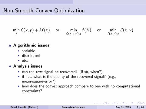
minxL(x , y) + λf (x) or min
L(x ,y)≤c1
f (X ) or minf (x)≤c2
L(x , y)
Algorithmic issues:I scalableI distributedI etc.
Analysis issues:I can the true signal be recovered? (if so, when?)I if not, what is the quality of the recovered signal? (e.g.,
mean-square-error?)I how does the convex approach compare to one with no computational
constraints?I how to choose the regularizer λ ≥ 0? (or the constraint bounds c1 and
c2?)
Babak Hassibi (Caltech) Comparison Lemmas Aug 31, 2015 6 / 65

Non-Smooth Convex Optimization
minxL(x , y) + λf (x) or min
L(x ,y)≤c1
f (X ) or minf (x)≤c2
L(x , y)
Algorithmic issues:I scalableI distributedI etc.
Analysis issues:I can the true signal be recovered? (if so, when?)
I if not, what is the quality of the recovered signal? (e.g.,mean-square-error?)
I how does the convex approach compare to one with no computationalconstraints?
I how to choose the regularizer λ ≥ 0? (or the constraint bounds c1 andc2?)
Babak Hassibi (Caltech) Comparison Lemmas Aug 31, 2015 6 / 65
Non-Smooth Convex Optimization
minxL(x , y) + λf (x) or min
L(x ,y)≤c1
f (X ) or minf (x)≤c2
L(x , y)
Algorithmic issues:I scalableI distributedI etc.
Analysis issues:I can the true signal be recovered? (if so, when?)I if not, what is the quality of the recovered signal? (e.g.,
mean-square-error?)
I how does the convex approach compare to one with no computationalconstraints?
I how to choose the regularizer λ ≥ 0? (or the constraint bounds c1 andc2?)
Babak Hassibi (Caltech) Comparison Lemmas Aug 31, 2015 6 / 65
Non-Smooth Convex Optimization
minxL(x , y) + λf (x) or min
L(x ,y)≤c1
f (X ) or minf (x)≤c2
L(x , y)
Algorithmic issues:I scalableI distributedI etc.
Analysis issues:I can the true signal be recovered? (if so, when?)I if not, what is the quality of the recovered signal? (e.g.,
mean-square-error?)I how does the convex approach compare to one with no computational
constraints?
I how to choose the regularizer λ ≥ 0? (or the constraint bounds c1 andc2?)
Babak Hassibi (Caltech) Comparison Lemmas Aug 31, 2015 6 / 65

Non-Smooth Convex Optimization
minxL(x , y) + λf (x) or min
L(x ,y)≤c1
f (X ) or minf (x)≤c2
L(x , y)
Algorithmic issues:I scalableI distributedI etc.
Analysis issues:I can the true signal be recovered? (if so, when?)I if not, what is the quality of the recovered signal? (e.g.,
mean-square-error?)I how does the convex approach compare to one with no computational
constraints?I how to choose the regularizer λ ≥ 0? (or the constraint bounds c1 and
c2?)
Babak Hassibi (Caltech) Comparison Lemmas Aug 31, 2015 6 / 65
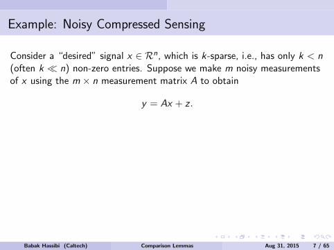
Example: Noisy Compressed Sensing
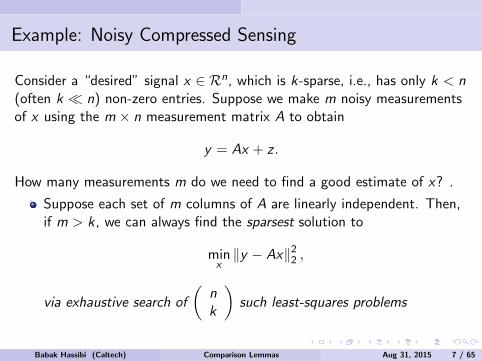
Consider a “desired” signal x ∈ Rn, which is k-sparse, i.e., has only k < n(often k n) non-zero entries. Suppose we make m noisy measurementsof x using the m × n measurement matrix A to obtain
y = Ax + z .
How many measurements m do we need to find a good estimate of x? .
Suppose each set of m columns of A are linearly independent. Then,if m > k , we can always find the sparsest solution to
minx‖y − Ax‖2
2 ,
via exhaustive search of
(nk
)such least-squares problems
Babak Hassibi (Caltech) Comparison Lemmas Aug 31, 2015 7 / 65

Example: Noisy Compressed Sensing
Consider a “desired” signal x ∈ Rn, which is k-sparse, i.e., has only k < n(often k n) non-zero entries. Suppose we make m noisy measurementsof x using the m × n measurement matrix A to obtain
y = Ax + z .
How many measurements m do we need to find a good estimate of x?
.
Suppose each set of m columns of A are linearly independent. Then,if m > k , we can always find the sparsest solution to
minx‖y − Ax‖2
2 ,
via exhaustive search of
(nk
)such least-squares problems
Babak Hassibi (Caltech) Comparison Lemmas Aug 31, 2015 7 / 65
Example: Noisy Compressed Sensing
Consider a “desired” signal x ∈ Rn, which is k-sparse, i.e., has only k < n(often k n) non-zero entries. Suppose we make m noisy measurementsof x using the m × n measurement matrix A to obtain
y = Ax + z .
How many measurements m do we need to find a good estimate of x? .
Suppose each set of m columns of A are linearly independent. Then,if m > k , we can always find the sparsest solution to
minx‖y − Ax‖2
2 ,
via exhaustive search of
(nk
)such least-squares problems
Babak Hassibi (Caltech) Comparison Lemmas Aug 31, 2015 7 / 65

Example: Noisy Compressed Sensing
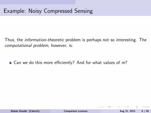
Thus, the information-theoretic problem is perhaps not so interesting.
Thecomputational problem, however, is:
Can we do this more efficiently? And for what values of m?
What about problems (such as low rank matrix recovery) where it isnot possible to enumerate all structured signals?
Babak Hassibi (Caltech) Comparison Lemmas Aug 31, 2015 8 / 65

Example: Noisy Compressed Sensing
Thus, the information-theoretic problem is perhaps not so interesting. Thecomputational problem, however, is:
Can we do this more efficiently? And for what values of m?
What about problems (such as low rank matrix recovery) where it isnot possible to enumerate all structured signals?
Babak Hassibi (Caltech) Comparison Lemmas Aug 31, 2015 8 / 65

LASSO
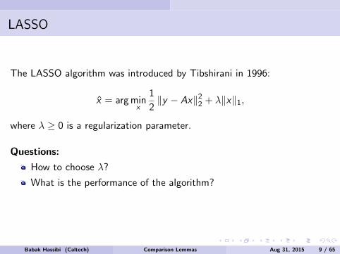
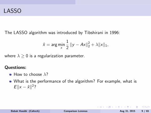
The LASSO algorithm was introduced by Tibshirani in 1996:
x = arg minx
1
2‖y − Ax‖2
2 + λ‖x‖1,
where λ ≥ 0 is a regularization parameter.
Questions:
How to choose λ?
What is the performance of the algorithm? For example, what isE‖x − x‖2?
Babak Hassibi (Caltech) Comparison Lemmas Aug 31, 2015 9 / 65

LASSO
The LASSO algorithm was introduced by Tibshirani in 1996:
x = arg minx
1
2‖y − Ax‖2
2 + λ‖x‖1,
where λ ≥ 0 is a regularization parameter.
Questions:
How to choose λ?
What is the performance of the algorithm? For example, what isE‖x − x‖2?
Babak Hassibi (Caltech) Comparison Lemmas Aug 31, 2015 9 / 65
LASSO
The LASSO algorithm was introduced by Tibshirani in 1996:
x = arg minx
1
2‖y − Ax‖2
2 + λ‖x‖1,
where λ ≥ 0 is a regularization parameter.
Questions:
How to choose λ?
What is the performance of the algorithm?
For example, what isE‖x − x‖2?
Babak Hassibi (Caltech) Comparison Lemmas Aug 31, 2015 9 / 65
LASSO
The LASSO algorithm was introduced by Tibshirani in 1996:
x = arg minx
1
2‖y − Ax‖2
2 + λ‖x‖1,
where λ ≥ 0 is a regularization parameter.
Questions:
How to choose λ?
What is the performance of the algorithm? For example, what isE‖x − x‖2?
Babak Hassibi (Caltech) Comparison Lemmas Aug 31, 2015 9 / 65

Generalized LASSO
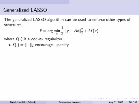
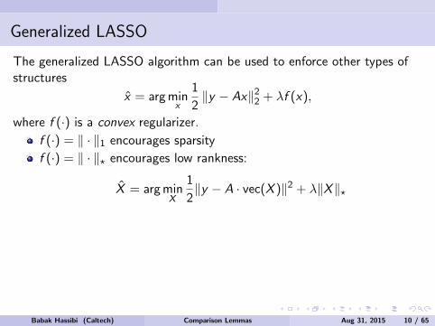
The generalized LASSO algorithm can be used to enforce other types ofstructures
x = arg minx
1
2‖y − Ax‖2
2 + λf (x),
where f (·) is a convex regularizer.
f (·) = ‖ · ‖1 encourages sparsity
f (·) = ‖ · ‖? encourages low rankness:
X = arg minX
1
2‖y − A · vec(X )‖2 + λ‖X‖?
f (·) = ‖ · ‖1,2 (the mixed `1/`2 norm) encourages block-sparsity
‖x‖1,2 =∑b
‖xb‖2.
etc.
Babak Hassibi (Caltech) Comparison Lemmas Aug 31, 2015 10 / 65
Generalized LASSO
The generalized LASSO algorithm can be used to enforce other types ofstructures
x = arg minx
1
2‖y − Ax‖2
2 + λf (x),
where f (·) is a convex regularizer.
f (·) = ‖ · ‖1 encourages sparsity
f (·) = ‖ · ‖? encourages low rankness:
X = arg minX
1
2‖y − A · vec(X )‖2 + λ‖X‖?
f (·) = ‖ · ‖1,2 (the mixed `1/`2 norm) encourages block-sparsity
‖x‖1,2 =∑b
‖xb‖2.
etc.
Babak Hassibi (Caltech) Comparison Lemmas Aug 31, 2015 10 / 65

Generalized LASSO
The generalized LASSO algorithm can be used to enforce other types ofstructures
x = arg minx
1
2‖y − Ax‖2
2 + λf (x),
where f (·) is a convex regularizer.
f (·) = ‖ · ‖1 encourages sparsity
f (·) = ‖ · ‖? encourages low rankness:
X = arg minX
1
2‖y − A · vec(X )‖2 + λ‖X‖?
f (·) = ‖ · ‖1,2 (the mixed `1/`2 norm) encourages block-sparsity
‖x‖1,2 =∑b
‖xb‖2.
etc.Babak Hassibi (Caltech) Comparison Lemmas Aug 31, 2015 10 / 65

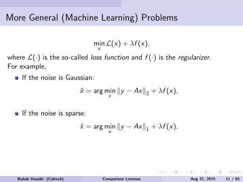
More General (Machine Learning) Problems
minxL(x) + λf (x),
where L(·) is the so-called loss function and f (·) is the regularizer.
For example,
If the noise is Gaussian:
x = arg minx‖y − Ax‖2 + λf (x),
If the noise is sparse:
x = arg minx‖y − Ax‖1 + λf (x),
If the noise is bounded:
x = arg minx‖y − Ax‖∞ + λf (x),
Babak Hassibi (Caltech) Comparison Lemmas Aug 31, 2015 11 / 65

More General (Machine Learning) Problems
minxL(x) + λf (x),
where L(·) is the so-called loss function and f (·) is the regularizer.For example,
If the noise is Gaussian:
x = arg minx‖y − Ax‖2 + λf (x),
If the noise is sparse:
x = arg minx‖y − Ax‖1 + λf (x),
If the noise is bounded:
x = arg minx‖y − Ax‖∞ + λf (x),
Babak Hassibi (Caltech) Comparison Lemmas Aug 31, 2015 11 / 65

The Squared Error of Generalized LASSO
x = arg minx‖y − Ax‖2 + λf (x)
The LASSO algorithm has been extensively studied
However, most performance bounds are rather loose
Can we compute E‖x − x‖2? Can we determine the optimal λ?
Turns out we can. But to do so, we need to tell an earlier story....
Babak Hassibi (Caltech) Comparison Lemmas Aug 31, 2015 12 / 65

The Squared Error of Generalized LASSO
x = arg minx‖y − Ax‖2 + λf (x)
The LASSO algorithm has been extensively studied
However, most performance bounds are rather loose
Can we compute E‖x − x‖2?
Can we determine the optimal λ?
Turns out we can. But to do so, we need to tell an earlier story....
Babak Hassibi (Caltech) Comparison Lemmas Aug 31, 2015 12 / 65

The Squared Error of Generalized LASSO
x = arg minx‖y − Ax‖2 + λf (x)
The LASSO algorithm has been extensively studied
However, most performance bounds are rather loose
Can we compute E‖x − x‖2? Can we determine the optimal λ?
Turns out we can. But to do so, we need to tell an earlier story....
Babak Hassibi (Caltech) Comparison Lemmas Aug 31, 2015 12 / 65
The Squared Error of Generalized LASSO
x = arg minx‖y − Ax‖2 + λf (x)
The LASSO algorithm has been extensively studied
However, most performance bounds are rather loose
Can we compute E‖x − x‖2? Can we determine the optimal λ?
Turns out we can.
But to do so, we need to tell an earlier story....
Babak Hassibi (Caltech) Comparison Lemmas Aug 31, 2015 12 / 65

The Squared Error of Generalized LASSO
x = arg minx‖y − Ax‖2 + λf (x)
The LASSO algorithm has been extensively studied
However, most performance bounds are rather loose
Can we compute E‖x − x‖2? Can we determine the optimal λ?
Turns out we can. But to do so, we need to tell an earlier story....
Babak Hassibi (Caltech) Comparison Lemmas Aug 31, 2015 12 / 65
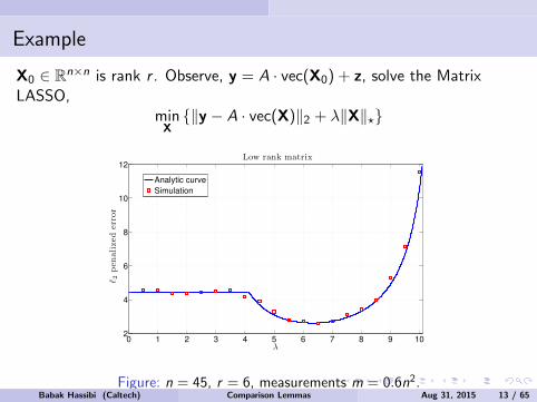
Example
X0 ∈ Rn×n is rank r . Observe, y = A · vec(X0) + z, solve the MatrixLASSO,
minX‖y − A · vec(X)‖2 + λ‖X‖?
0 1 2 3 4 5 6 7 8 9 102
4
6
8
10
12Low rank matrix
λ
ℓ 2pen
alize
der
ror
Analytic curve
Simulation
Figure: n = 45, r = 6, measurements m = 0.6n2.Babak Hassibi (Caltech) Comparison Lemmas Aug 31, 2015 13 / 65

Noiseless Compressed Sensing
Consider a “desired” signal x ∈ Rn, which is k-sparse, i.e., has only k < n(often k n) non-zero entries. Suppose we make m measurements of xusing the m × n measurement matrix A to obtain
y = Ax .
A heuristic (that has been around for decades) is:
min ‖x‖1 subject to y = Ax
The seminal work of Candes and Tao (2004) and Donoho (2004) hasshown that under certain conditions the above `1 optimization can exactlyrecover the solution, thus avoiding an exponential search.
Candes and Tao showed that if A satisfies certain restricted isometryconditions, then `1 optimization works for small enough k
I gives “order optimal”, but very loose bounds
Babak Hassibi (Caltech) Comparison Lemmas Aug 31, 2015 14 / 65
Exact Conditions for Signal Recovery
We will consider a general framework.
Consider a structured signal x0, with a structure-inducing norm f (·) = ‖ · ‖.We have access to linear measurements y = A(x0) ∈ Rm, and would liketo know when we can recover the signal x0 from the convex problem
min ‖x‖ subject to A(x) = A(x0)?
For sparse signals we have the `1 norm; for nonuniform sparse signalsthe weighted `1 norm; for low rank matrices the nuclear norm
Let U(x0) = z , ‖x0 + z‖ ≤ ‖x0‖. Then x0 is the unique solution of theabove convex problem iff:
N (A) ∩ U(x0) = 0.
Babak Hassibi (Caltech) Comparison Lemmas Aug 31, 2015 15 / 65

A Bit of Geometry: Subgradients and the Polar Cone
Note that N (A) is a linear subspace and that therefore the condition canbe rewritten as
N (A) ∩ cone(U(x0)) = 0.
We can characterize cone(U(x0)) through the subgradient of the convexfunction ‖ · ‖:
∂‖x0‖ = v |vT (x − x0) + ‖x0‖ ≤ ‖x‖,∀x.
Babak Hassibi (Caltech) Comparison Lemmas Aug 31, 2015 16 / 65

A Bit of Geometry: Subgradients and the Polar Cone
Note that N (A) is a linear subspace and that therefore the condition canbe rewritten as
N (A) ∩ cone(U(x0)) = 0.
We can characterize cone(U(x0)) through the subgradient of the convexfunction ‖ · ‖:
∂‖x0‖ = v |vT (x − x0) + ‖x0‖ ≤ ‖x‖, ∀x.
Babak Hassibi (Caltech) Comparison Lemmas Aug 31, 2015 16 / 65

A Bit of Geometry: Subgradients and the Polar Cone
It is now straightforward to see that
cone(U(x0)) = z |vT z ≤ 0, ∀v ∈ ∂‖x0‖.
But this is simply the polar cone of ∂‖x0‖.
Thus, we can recover x0 from the convex problem iff:
N (A) ∩ (∂‖x0‖)O = 0.
Babak Hassibi (Caltech) Comparison Lemmas Aug 31, 2015 17 / 65

Phase Transitions for Exact Signal Recovery
Thus, recovery depends on the null space of the measurement matrixand the polar cone of the subgradient (at the point we want torecover).
While computing the polar cone of the subgradient is oftenstraightforward, checking the condition N (A) ∩ (∂‖x0‖)O = 0 for aspecific A is difficult.
Therefore the focus has been on checking whether the condition holdsfor a family of random A’s with high probability.
It is customary to assume that the measurement matrix A iscomposed of iid zero-mean unit-variance entries.
This makes the nullspace N (A) rotationally-invariant.
The probability that a rotationally-invariant subspace intersects acone is called the Grassman angle of the cone.
Babak Hassibi (Caltech) Comparison Lemmas Aug 31, 2015 18 / 65

Phase Transitions for Convex Relaxation - Some History
In the `1 case the subgradient cone is polyhedral and Donoho andTanner (2005) computed the Grassman angle to obtain the minimumnumber of measurements required to recover a k-sparse signal
I very cumbersome calculations, required considering exponentially manyinner and outer angles, etc.
Extended to robustness and weighted `1 by Xu-H in 2007 (even morecumbersome)
Donoho-Tanner approach hard to extend (Recht-Xu-H (2008)attempted this for nuclear norm—only obtained bounds sincesubgradient cone is non-polyhedral)
New framework developed by Rudelson and Vershynin (2006) and,especially, Stojnic in 2009 (using escape-through-mesh and Gaussianwidths)
I rederived results for sparse vectors; new results for block-sparse vectorsI much simpler derivation
Babak Hassibi (Caltech) Comparison Lemmas Aug 31, 2015 19 / 65

Phase Transitions for Convex Relaxation - Some History
In the `1 case the subgradient cone is polyhedral and Donoho andTanner (2005) computed the Grassman angle to obtain the minimumnumber of measurements required to recover a k-sparse signal
I very cumbersome calculations, required considering exponentially manyinner and outer angles, etc.
Extended to robustness and weighted `1 by Xu-H in 2007 (even morecumbersome)
Donoho-Tanner approach hard to extend (Recht-Xu-H (2008)attempted this for nuclear norm—only obtained bounds sincesubgradient cone is non-polyhedral)
New framework developed by Rudelson and Vershynin (2006) and,especially, Stojnic in 2009 (using escape-through-mesh and Gaussianwidths)
I rederived results for sparse vectors; new results for block-sparse vectors
I much simpler derivation
Babak Hassibi (Caltech) Comparison Lemmas Aug 31, 2015 19 / 65

Phase Transitions for Convex Relaxation - Some History
In the `1 case the subgradient cone is polyhedral and Donoho andTanner (2005) computed the Grassman angle to obtain the minimumnumber of measurements required to recover a k-sparse signal
I very cumbersome calculations, required considering exponentially manyinner and outer angles, etc.
Extended to robustness and weighted `1 by Xu-H in 2007 (even morecumbersome)
Donoho-Tanner approach hard to extend (Recht-Xu-H (2008)attempted this for nuclear norm—only obtained bounds sincesubgradient cone is non-polyhedral)
New framework developed by Rudelson and Vershynin (2006) and,especially, Stojnic in 2009 (using escape-through-mesh and Gaussianwidths)
I rederived results for sparse vectors; new results for block-sparse vectorsI much simpler derivation
Babak Hassibi (Caltech) Comparison Lemmas Aug 31, 2015 19 / 65

Phase Transitions for Convex Relaxation - Some History
Stojnic’s new approach:
Allowed the development of a general framework(Chandrasekaran-Parrilo-Willsky, 2010)
I exact calculation for nuclear norm (Oymak-H, 2010)
Deconvolution (McCoy-Tropp, 2012)
Tightness of Gaussian widths Stojnic, 2013 (for `1),Amelunxen-Lotz-McCoy-Tropp, 2013 (for the general case)
Replica-based analysis:
Guo, Baron and Shamai (2009), Kabashima, Wadayama, Tanaka(2009), Rangan, Fletecher, Goyal (2012), Vehkapera, Kabashima,Chatterjee (2013), Wen, Zhang, Wong, Chen (2014)
Babak Hassibi (Caltech) Comparison Lemmas Aug 31, 2015 20 / 65
What About the Noisy Case?
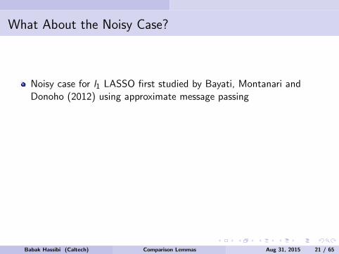
Noisy case for l1 LASSO first studied by Bayati, Montanari andDonoho (2012) using approximate message passing
A new approach developed by Stojnic (2013)
Our approach is inspired by Stojnic (2013)I subsumes all earlier (noiseless and noisy results)I allows for much, much moreI is the most natural way to study the problem
Where does all this come from?
Babak Hassibi (Caltech) Comparison Lemmas Aug 31, 2015 21 / 65
What About the Noisy Case?
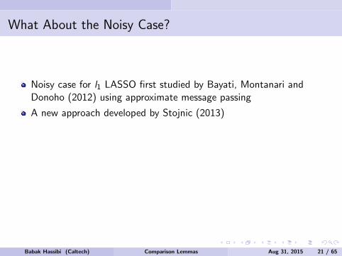
Noisy case for l1 LASSO first studied by Bayati, Montanari andDonoho (2012) using approximate message passing
A new approach developed by Stojnic (2013)
Our approach is inspired by Stojnic (2013)I subsumes all earlier (noiseless and noisy results)I allows for much, much moreI is the most natural way to study the problem
Where does all this come from?
Babak Hassibi (Caltech) Comparison Lemmas Aug 31, 2015 21 / 65
What About the Noisy Case?
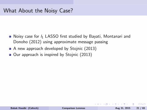
Noisy case for l1 LASSO first studied by Bayati, Montanari andDonoho (2012) using approximate message passing
A new approach developed by Stojnic (2013)
Our approach is inspired by Stojnic (2013)
I subsumes all earlier (noiseless and noisy results)I allows for much, much moreI is the most natural way to study the problem
Where does all this come from?
Babak Hassibi (Caltech) Comparison Lemmas Aug 31, 2015 21 / 65

What About the Noisy Case?
Noisy case for l1 LASSO first studied by Bayati, Montanari andDonoho (2012) using approximate message passing
A new approach developed by Stojnic (2013)
Our approach is inspired by Stojnic (2013)I subsumes all earlier (noiseless and noisy results)I allows for much, much moreI is the most natural way to study the problem
Where does all this come from?
Babak Hassibi (Caltech) Comparison Lemmas Aug 31, 2015 21 / 65

Tribute to Dave Slepian (1923-2007)
David Slepian goes to a bar. What does the waitress say?
a. Claude just came in.
b. Will you be waiting for Jack?
c. Will you be attending the function?DS: What function?The prolate spheroidal wave function.DS: No, I am with a different group.
d. Will you be joining the French table?
e. XNone of the above. Would you care to compare our beers?
Babak Hassibi (Caltech) Comparison Lemmas Aug 31, 2015 22 / 65

Tribute to Dave Slepian (1923-2007)
David Slepian goes to a bar.
What does the waitress say?
a. Claude just came in.
b. Will you be waiting for Jack?
c. Will you be attending the function?DS: What function?The prolate spheroidal wave function.DS: No, I am with a different group.
d. Will you be joining the French table?
e. XNone of the above. Would you care to compare our beers?
Babak Hassibi (Caltech) Comparison Lemmas Aug 31, 2015 22 / 65

Tribute to Dave Slepian (1923-2007)
David Slepian goes to a bar. What does the waitress say?
a. Claude just came in.
b. Will you be waiting for Jack?
c. Will you be attending the function?DS: What function?The prolate spheroidal wave function.DS: No, I am with a different group.
d. Will you be joining the French table?
e. XNone of the above. Would you care to compare our beers?
Babak Hassibi (Caltech) Comparison Lemmas Aug 31, 2015 22 / 65

Tribute to Dave Slepian (1923-2007)
David Slepian goes to a bar. What does the waitress say?
a. Claude just came in.
b. Will you be waiting for Jack?
c. Will you be attending the function?
DS: What function?The prolate spheroidal wave function.DS: No, I am with a different group.
d. Will you be joining the French table?
e. XNone of the above. Would you care to compare our beers?
Babak Hassibi (Caltech) Comparison Lemmas Aug 31, 2015 22 / 65

Tribute to Dave Slepian (1923-2007)
David Slepian goes to a bar. What does the waitress say?
a. Claude just came in.
b. Will you be waiting for Jack?
c. Will you be attending the function?DS: What function?
The prolate spheroidal wave function.DS: No, I am with a different group.
d. Will you be joining the French table?
e. XNone of the above. Would you care to compare our beers?
Babak Hassibi (Caltech) Comparison Lemmas Aug 31, 2015 22 / 65

Tribute to Dave Slepian (1923-2007)
David Slepian goes to a bar. What does the waitress say?
a. Claude just came in.
b. Will you be waiting for Jack?
c. Will you be attending the function?DS: What function?The prolate spheroidal wave function.
DS: No, I am with a different group.
d. Will you be joining the French table?
e. XNone of the above. Would you care to compare our beers?
Babak Hassibi (Caltech) Comparison Lemmas Aug 31, 2015 22 / 65

Tribute to Dave Slepian (1923-2007)
David Slepian goes to a bar. What does the waitress say?
a. Claude just came in.
b. Will you be waiting for Jack?
c. Will you be attending the function?DS: What function?The prolate spheroidal wave function.DS: No, I am with a different group.
d. Will you be joining the French table?
e. XNone of the above. Would you care to compare our beers?
Babak Hassibi (Caltech) Comparison Lemmas Aug 31, 2015 22 / 65

Tribute to Dave Slepian (1923-2007)
David Slepian goes to a bar. What does the waitress say?
a. Claude just came in.
b. Will you be waiting for Jack?
c. Will you be attending the function?DS: What function?The prolate spheroidal wave function.DS: No, I am with a different group.
d. Will you be joining the French table?
e. XNone of the above.
Would you care to compare our beers?
Babak Hassibi (Caltech) Comparison Lemmas Aug 31, 2015 22 / 65

Tribute to Dave Slepian (1923-2007)
David Slepian goes to a bar. What does the waitress say?
a. Claude just came in.
b. Will you be waiting for Jack?
c. Will you be attending the function?DS: What function?The prolate spheroidal wave function.DS: No, I am with a different group.
d. Will you be joining the French table?
e. XNone of the above. Would you care to compare our beers?
Babak Hassibi (Caltech) Comparison Lemmas Aug 31, 2015 22 / 65

Slepian’s Comparison Lemma (1962)
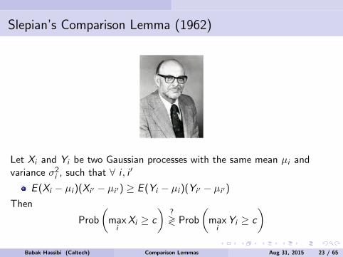
Let Xi and Yi be two Gaussian processes with the same mean µi andvariance σ2
i , such that ∀ i , i ′
E (Xi − µi )(Xi ′ − µi ′) ≥ E (Yi − µi )(Yi ′ − µi ′)Then
Prob
(max
iXi ≥ c
)?≷ Prob
(max
iYi ≥ c
)
Babak Hassibi (Caltech) Comparison Lemmas Aug 31, 2015 23 / 65

Slepian’s Comparison Lemma (1962)
Let Xi and Yi be two Gaussian processes with the same mean µi andvariance σ2
i , such that ∀ i , i ′
E (Xi − µi )(Xi ′ − µi ′) ≥ E (Yi − µi )(Yi ′ − µi ′)Then
Prob
(max
iXi ≥ c
)?≷ Prob
(max
iYi ≥ c
)
Babak Hassibi (Caltech) Comparison Lemmas Aug 31, 2015 23 / 65
Slepian’s Comparison Lemma (1962)
Let Xi and Yi be two Gaussian processes with the same mean µi andvariance σ2
i , such that ∀ i , i ′
E (Xi − µi )(Xi ′ − µi ′) ≥ E (Yi − µi )(Yi ′ − µi ′)Then
Prob
(max
iXi ≥ c
)?≷ Prob
(max
iYi ≥ c
)Babak Hassibi (Caltech) Comparison Lemmas Aug 31, 2015 23 / 65

Slepian’s Comparison Lemma (1962)
Let Xi and Yi be two Gaussian processes with the same mean µi andvariance σ2
i , such that ∀ i , i ′
E (Xi − µi )(Xi ′ − µi ′) ≥ E (Yi − µi )(Yi ′ − µi ′)Then
Prob
(max
iXi ≥ c
)≤ Prob
(max
iYi ≥ c
)Babak Hassibi (Caltech) Comparison Lemmas Aug 31, 2015 24 / 65

Slepian’s Comparison Lemma (1962)
proof not too difficult, but not trivial, either
lemma not generally true for non-Gaussian processes
Babak Hassibi (Caltech) Comparison Lemmas Aug 31, 2015 25 / 65
Maximum Singular Value of a Gaussian Matrix
What is this good for?
Let A ∈ Rm×n be a matrix with iid N(0, 1) entries and consider itsmaximum singular value:
σmax(A) = ‖A‖ = max‖u‖=1
max‖v‖=1
uTAv .
Define the two Gaussian processes
Xuv = uTAv + γ and Yuv = uTg + vTh,
where γ ∈ R, g ∈ Rm and h ∈ Rn have iid N(0, 1) entries. Then it is nothard to see that both processes have zero mean and variance 2.
Babak Hassibi (Caltech) Comparison Lemmas Aug 31, 2015 26 / 65
Maximum Singular Value of a Gaussian Matrix
What is this good for?
Let A ∈ Rm×n be a matrix with iid N(0, 1) entries and consider itsmaximum singular value:
σmax(A) = ‖A‖ = max‖u‖=1
max‖v‖=1
uTAv .
Define the two Gaussian processes
Xuv = uTAv + γ and Yuv = uTg + vTh,
where γ ∈ R, g ∈ Rm and h ∈ Rn have iid N(0, 1) entries.
Then it is nothard to see that both processes have zero mean and variance 2.
Babak Hassibi (Caltech) Comparison Lemmas Aug 31, 2015 26 / 65

Maximum Singular Value of a Gaussian Matrix
What is this good for?
Let A ∈ Rm×n be a matrix with iid N(0, 1) entries and consider itsmaximum singular value:
σmax(A) = ‖A‖ = max‖u‖=1
max‖v‖=1
uTAv .
Define the two Gaussian processes
Xuv = uTAv + γ and Yuv = uTg + vTh,
where γ ∈ R, g ∈ Rm and h ∈ Rn have iid N(0, 1) entries. Then it is nothard to see that both processes have zero mean and variance 2.
Babak Hassibi (Caltech) Comparison Lemmas Aug 31, 2015 26 / 65
Maximum Singular Value of a Gaussian Matrix
Xuv = uTAv + γ and Yuv = uTg + vTh,
Now,
EXuvXu′v ′−EYuvYu′v ′ = uTu′vT v ′+1−uTu′−vT v ′ = (1−uTu′)(1−vT v ′) ≥ 0.
Therefore from Slepian’s lemma:
Prob
(max‖u‖=1
max‖v‖=1
uTAv + γ ≥ c
)︸ ︷︷ ︸
≥ 12Prob(‖A‖≥c)
≤ Prob
(max‖u‖=1
max‖v‖=1
uTg + vTh ≥ c
)︸ ︷︷ ︸
Prob(‖g‖+‖h‖≥c)
.
Since ‖g‖+ ‖h‖ concentrates around√m +
√n, this implies that the
probability that ‖A‖ (significantly) exceeds√m +
√n is very small.
Babak Hassibi (Caltech) Comparison Lemmas Aug 31, 2015 27 / 65
Minimum Singular Value of a Gaussian Matrix
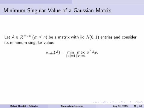
Let A ∈ Rm×n (m ≤ n) be a matrix with iid N(0, 1) entries and considerits minimum singular value:
σmin(A) = min‖u‖=1
max‖v‖=1
uTAv .
Slepian’s lemma does not apply.
It took 24 years for there to be progress...
Babak Hassibi (Caltech) Comparison Lemmas Aug 31, 2015 28 / 65

Minimum Singular Value of a Gaussian Matrix
Let A ∈ Rm×n (m ≤ n) be a matrix with iid N(0, 1) entries and considerits minimum singular value:
σmin(A) = min‖u‖=1
max‖v‖=1
uTAv .
Slepian’s lemma does not apply.
It took 24 years for there to be progress...
Babak Hassibi (Caltech) Comparison Lemmas Aug 31, 2015 28 / 65

Gordon’s Comparison Lemma (1988)
Let Xij and Yij be two Gaussian processes with the same mean µij andvariance σ2
ij , such that ∀ i , j , i ′, j ′
1 E (Xij − µij)(Xij ′ − µij ′) ≤ E (Yij − µij)(Yij ′ − µij ′)2 E (Xij − µij)(Xi ′j ′ − µi ′j ′) ≥ E (Yij − µij)(Yi ′j ′ − µi ′j ′)
Then
Prob
(mini
maxj
Xij ≤ c
)?≷ Prob
(mini
maxj
Yij ≤ c
)Babak Hassibi (Caltech) Comparison Lemmas Aug 31, 2015 29 / 65

Gordon’s Comparison Lemma (1988)
Let Xij and Yij be two Gaussian processes with the same mean µij andvariance σ2
ij , such that ∀ i , j , i ′, j ′
1 E (Xij − µij)(Xij ′ − µij ′) ≤ E (Yij − µij)(Yij ′ − µij ′)2 E (Xij − µij)(Xi ′j ′ − µi ′j ′) ≥ E (Yij − µij)(Yi ′j ′ − µi ′j ′)
Then
Prob
(mini
maxj
Xij ≤ c
)≤ Prob
(mini
maxj
Yij ≤ c
)Babak Hassibi (Caltech) Comparison Lemmas Aug 31, 2015 30 / 65

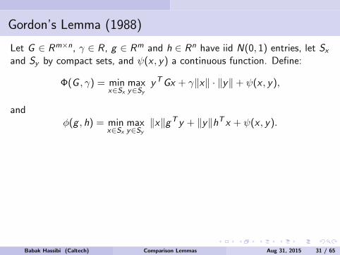
Gordon’s Lemma (1988)
Let G ∈ Rm×n, γ ∈ R, g ∈ Rm and h ∈ Rn have iid N(0, 1) entries, let Sxand Sy by compact sets, and ψ(x , y) a continuous function.
Define:
Φ(G , γ) = minx∈Sx
maxy∈Sy
yTGx + γ‖x‖ · ‖y‖+ ψ(x , y),
andφ(g , h) = min
x∈Sxmaxy∈Sy
‖x‖gT y + ‖y‖hT x + ψ(x , y).
Then it holds that:
Prob(Φ(G , γ) ≤ c) ≤ Prob(φ(g , h) ≤ c).
If c is a high probability lower bound on φ(·, ·), same is true of Φ(·, ·)Basis for “escape through mesh” and “Gaussian width”
Can be used to show that σmin(A) behaves as√n −√m
Babak Hassibi (Caltech) Comparison Lemmas Aug 31, 2015 31 / 65
Gordon’s Lemma (1988)
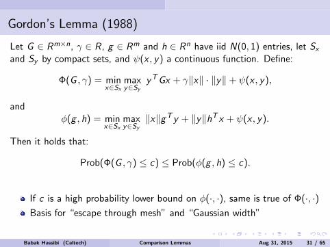
Let G ∈ Rm×n, γ ∈ R, g ∈ Rm and h ∈ Rn have iid N(0, 1) entries, let Sxand Sy by compact sets, and ψ(x , y) a continuous function. Define:
Φ(G , γ) = minx∈Sx
maxy∈Sy
yTGx + γ‖x‖ · ‖y‖+ ψ(x , y),
andφ(g , h) = min
x∈Sxmaxy∈Sy
‖x‖gT y + ‖y‖hT x + ψ(x , y).
Then it holds that:
Prob(Φ(G , γ) ≤ c) ≤ Prob(φ(g , h) ≤ c).
If c is a high probability lower bound on φ(·, ·), same is true of Φ(·, ·)Basis for “escape through mesh” and “Gaussian width”
Can be used to show that σmin(A) behaves as√n −√m
Babak Hassibi (Caltech) Comparison Lemmas Aug 31, 2015 31 / 65

Gordon’s Lemma (1988)
Let G ∈ Rm×n, γ ∈ R, g ∈ Rm and h ∈ Rn have iid N(0, 1) entries, let Sxand Sy by compact sets, and ψ(x , y) a continuous function. Define:
Φ(G , γ) = minx∈Sx
maxy∈Sy
yTGx + γ‖x‖ · ‖y‖+ ψ(x , y),
andφ(g , h) = min
x∈Sxmaxy∈Sy
‖x‖gT y + ‖y‖hT x + ψ(x , y).
Then it holds that:
Prob(Φ(G , γ) ≤ c) ≤ Prob(φ(g , h) ≤ c).
If c is a high probability lower bound on φ(·, ·), same is true of Φ(·, ·)
Basis for “escape through mesh” and “Gaussian width”
Can be used to show that σmin(A) behaves as√n −√m
Babak Hassibi (Caltech) Comparison Lemmas Aug 31, 2015 31 / 65
Gordon’s Lemma (1988)
Let G ∈ Rm×n, γ ∈ R, g ∈ Rm and h ∈ Rn have iid N(0, 1) entries, let Sxand Sy by compact sets, and ψ(x , y) a continuous function. Define:
Φ(G , γ) = minx∈Sx
maxy∈Sy
yTGx + γ‖x‖ · ‖y‖+ ψ(x , y),
andφ(g , h) = min
x∈Sxmaxy∈Sy
‖x‖gT y + ‖y‖hT x + ψ(x , y).
Then it holds that:
Prob(Φ(G , γ) ≤ c) ≤ Prob(φ(g , h) ≤ c).
If c is a high probability lower bound on φ(·, ·), same is true of Φ(·, ·)Basis for “escape through mesh” and “Gaussian width”
Can be used to show that σmin(A) behaves as√n −√m
Babak Hassibi (Caltech) Comparison Lemmas Aug 31, 2015 31 / 65

Gordon’s Lemma (1988)
Let G ∈ Rm×n, γ ∈ R, g ∈ Rm and h ∈ Rn have iid N(0, 1) entries, let Sxand Sy by compact sets, and ψ(x , y) a continuous function. Define:
Φ(G , γ) = minx∈Sx
maxy∈Sy
yTGx + γ‖x‖ · ‖y‖+ ψ(x , y),
andφ(g , h) = min
x∈Sxmaxy∈Sy
‖x‖gT y + ‖y‖hT x + ψ(x , y).
Then it holds that:
Prob(Φ(G , γ) ≤ c) ≤ Prob(φ(g , h) ≤ c).
If c is a high probability lower bound on φ(·, ·), same is true of Φ(·, ·)Basis for “escape through mesh” and “Gaussian width”
Can be used to show that σmin(A) behaves as√n −√m
Babak Hassibi (Caltech) Comparison Lemmas Aug 31, 2015 31 / 65

A Stronger Version of Gordon’s Lemma (TOH 2014)
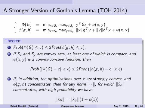
Φ(G ) = minx∈Sx maxy∈Sy yTGx + ψ(x , y)
φ(g , h) = minx∈Sx maxy∈Sy ‖x‖gT y + ‖y‖hT x + ψ(x , y)
Theorem1 Prob(Φ(G ) ≤ c) ≤ 2Prob(φ(g , h) ≤ c).
2 If Sx and Sy are convex sets, at least one of which is compact, andψ(x , y) is a convex-concave function, then
Prob (|Φ(G )− c | ≥ ε) ≤ 2Prob (|φ(g , h)− c | ≥ ε) .
3 If, in addition, the optimizations over x are strongly convex, andφ(g , h) concentrates, then for any norm ‖ · ‖, for which ‖xφ‖concentrates, with high probability we have
‖xΦ‖ = ‖xφ‖ (1 + o(1))
Babak Hassibi (Caltech) Comparison Lemmas Aug 31, 2015 32 / 65

A Stronger Version of Gordon’s Lemma (TOH 2014)
Φ(G ) = minx∈Sx maxy∈Sy yTGx + ψ(x , y)
φ(g , h) = minx∈Sx maxy∈Sy ‖x‖gT y + ‖y‖hT x + ψ(x , y)
Theorem1 Prob(Φ(G ) ≤ c) ≤ 2Prob(φ(g , h) ≤ c).
2 If Sx and Sy are convex sets, at least one of which is compact, andψ(x , y) is a convex-concave function, then
Prob (|Φ(G )− c | ≥ ε) ≤ 2Prob (|φ(g , h)− c | ≥ ε) .
3 If, in addition, the optimizations over x are strongly convex, andφ(g , h) concentrates, then for any norm ‖ · ‖, for which ‖xφ‖concentrates, with high probability we have
‖xΦ‖ = ‖xφ‖ (1 + o(1))
Babak Hassibi (Caltech) Comparison Lemmas Aug 31, 2015 32 / 65
Least-Squares
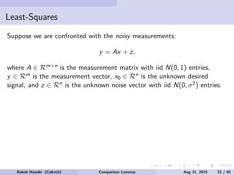
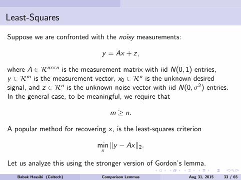
Suppose we are confronted with the noisy measurements:
y = Ax + z ,
where A ∈ Rm×n is the measurement matrix with iid N(0, 1) entries,y ∈ Rm is the measurement vector, x0 ∈ Rn is the unknown desiredsignal, and z ∈ Rn is the unknown noise vector with iid N(0, σ2) entries.
In the general case, to be meaningful, we require that
m ≥ n.
A popular method for recovering x , is the least-squares criterion
minx‖y − Ax‖2.
Let us analyze this using the stronger version of Gordon’s lemma.
Babak Hassibi (Caltech) Comparison Lemmas Aug 31, 2015 33 / 65

Least-Squares
Suppose we are confronted with the noisy measurements:
y = Ax + z ,
where A ∈ Rm×n is the measurement matrix with iid N(0, 1) entries,y ∈ Rm is the measurement vector, x0 ∈ Rn is the unknown desiredsignal, and z ∈ Rn is the unknown noise vector with iid N(0, σ2) entries.In the general case, to be meaningful, we require that
m ≥ n.
A popular method for recovering x , is the least-squares criterion
minx‖y − Ax‖2.
Let us analyze this using the stronger version of Gordon’s lemma.
Babak Hassibi (Caltech) Comparison Lemmas Aug 31, 2015 33 / 65

Least-Squares
To this end, define the estimation error w = x0 − x , so thaty − Ax = Aw + z .
Thus,
minx‖y − Ax‖2 = min
w‖Aw + z‖2
= minw
max‖u‖≤1
uT (Aw + z) = minw
max‖u‖≤1
uT[A 1
σ z] [ w
σ
].
This satisfies all the conditions of the lemma. The simpler optimization istherefore:
minw
max‖u‖≤1
√‖w‖2 + σ2gTu + ‖u‖
[hTw hσ
] [ wσ
],
where g = Rm, hw = Rn and hσ ∈ R have iid N(0, 1) entries.
Babak Hassibi (Caltech) Comparison Lemmas Aug 31, 2015 34 / 65

Least-Squares
To this end, define the estimation error w = x0 − x , so thaty − Ax = Aw + z . Thus,
minx‖y − Ax‖2 = min
w‖Aw + z‖2
= minw
max‖u‖≤1
uT (Aw + z) = minw
max‖u‖≤1
uT[A 1
σ z] [ w
σ
].
This satisfies all the conditions of the lemma.
The simpler optimization istherefore:
minw
max‖u‖≤1
√‖w‖2 + σ2gTu + ‖u‖
[hTw hσ
] [ wσ
],
where g = Rm, hw = Rn and hσ ∈ R have iid N(0, 1) entries.
Babak Hassibi (Caltech) Comparison Lemmas Aug 31, 2015 34 / 65

Least-Squares
To this end, define the estimation error w = x0 − x , so thaty − Ax = Aw + z . Thus,
minx‖y − Ax‖2 = min
w‖Aw + z‖2
= minw
max‖u‖≤1
uT (Aw + z) = minw
max‖u‖≤1
uT[A 1
σ z] [ w
σ
].
This satisfies all the conditions of the lemma. The simpler optimization istherefore:
minw
max‖u‖≤1
√‖w‖2 + σ2gTu + ‖u‖
[hTw hσ
] [ wσ
],
where g = Rm, hw = Rn and hσ ∈ R have iid N(0, 1) entries.
Babak Hassibi (Caltech) Comparison Lemmas Aug 31, 2015 34 / 65
Least-Squares
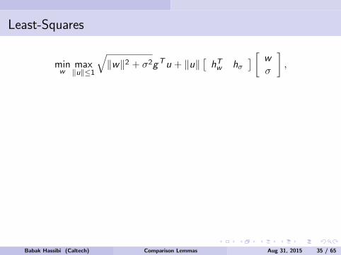
minw
max‖u‖≤1
√‖w‖2 + σ2gTu + ‖u‖
[hTw hσ
] [ wσ
],
The maximization over u is straightforward:
minw
√‖w‖2 + σ2‖g‖+ hTww + hσσ.
Fixing the norm of ‖w‖ = α, minimizing over the direction of w isstraightforward:
minα≥0
=√α2 + σ2‖g‖ − α‖hw‖+ hσσ.
Differentiating over α gives the solution:
α2
σ2=
‖hw‖2
‖g‖2 − ‖hw‖2→ n
m − n.
Babak Hassibi (Caltech) Comparison Lemmas Aug 31, 2015 35 / 65

Least-Squares
minw
max‖u‖≤1
√‖w‖2 + σ2gTu + ‖u‖
[hTw hσ
] [ wσ
],
The maximization over u is straightforward:
minw
√‖w‖2 + σ2‖g‖+ hTww + hσσ.
Fixing the norm of ‖w‖ = α, minimizing over the direction of w isstraightforward:
minα≥0
=√α2 + σ2‖g‖ − α‖hw‖+ hσσ.
Differentiating over α gives the solution:
α2
σ2=
‖hw‖2
‖g‖2 − ‖hw‖2→ n
m − n.
Babak Hassibi (Caltech) Comparison Lemmas Aug 31, 2015 35 / 65
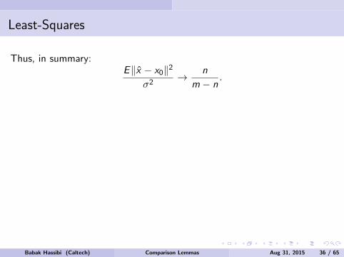
Least-Squares
Thus, in summary:E‖x − x0‖2
σ2→ n
m − n.
Of course, in the least-squares case, we need not use all this machinerysince the solutions are famously given by:
x =(ATA
)−1AT y and E‖x0 − x‖2
2 = σ2trace(ATA
)−1.
When A has iid N(0, 1) entries, ATA is a Wishart matrix whoseasymptotic eigendistribution is well known, from which we obtain
E‖x − x‖22
σ2→ n
m − n.
Babak Hassibi (Caltech) Comparison Lemmas Aug 31, 2015 36 / 65
Back to the Squared Error of Generalized LASSO
However, for generalized LASSO, we do not have closed form solutionsand the machinery becomes very useful:
x = arg minx‖y − Ax‖2 + λf (x)
Using the same argument as before, we obtain the simpler optimizationproblem:
minw
max‖u‖≤1
√‖w‖2 + σ2gTu + ‖u‖
[hTw hσ
] [ wσ
]+ λf (x0 − w).
Or:
minw
√‖w‖2 + σ2‖g‖+ hTww + hσσ + λf (x0 − w).
Babak Hassibi (Caltech) Comparison Lemmas Aug 31, 2015 37 / 65

Squared Error of Generalized LASSO
minw
√‖w‖2 + σ2‖g‖+ hTww + hσσ + λf (x0 − w).
While this can be analyzed in this generality, it is instructive to focus onthe low noise, σ → 0, case.
Here ‖w‖ will be small and we may thereforewrite
f (x0 − w) & f (x0) + sups∈∂f (x0)
sT (−w),
so that we obtain
minw
√‖w‖2 + σ2‖g‖+ hTww + hσσ + λ sup
s∈∂f (x0)sT (−w),
or
minw
√‖w‖2 + σ2‖g‖+ sup
s∈λ∂f (x0)(hw − s)Tw .
Babak Hassibi (Caltech) Comparison Lemmas Aug 31, 2015 38 / 65

Squared Error of Generalized LASSO
minw
√‖w‖2 + σ2‖g‖+ hTww + hσσ + λf (x0 − w).
While this can be analyzed in this generality, it is instructive to focus onthe low noise, σ → 0, case. Here ‖w‖ will be small and we may thereforewrite
f (x0 − w) & f (x0) + sups∈∂f (x0)
sT (−w),
so that we obtain
minw
√‖w‖2 + σ2‖g‖+ hTww + hσσ + λ sup
s∈∂f (x0)sT (−w),
or
minw
√‖w‖2 + σ2‖g‖+ sup
s∈λ∂f (x0)(hw − s)Tw .
Babak Hassibi (Caltech) Comparison Lemmas Aug 31, 2015 38 / 65

Squared Error of Generalized LASSO
minw
√‖w‖2 + σ2‖g‖+ sup
s∈λ∂f (x0)(hw − s)Tw .
As before, fixing the norm ‖w‖ = α, optimization over the direction of wis straightforward:
minα≥0
√α2 + σ2‖g‖+ sup
s∈λ∂f (x0)−α‖hw − s‖.
Or:minα≥0
√α2 + σ2‖g‖ − α inf
s∈λ∂f (x0)‖hw − s‖︸ ︷︷ ︸
dist(hw ,λ∂f (x0))
.
Differentiating over α yields:
limσ→0
α2
σ2=
dist2(hw , λ∂f (x0))
m − dist2(hw , λ∂f (x0)).
Babak Hassibi (Caltech) Comparison Lemmas Aug 31, 2015 39 / 65

Main Result: The Squared Error of Generalized LASSO
Generate an n-dimensional vector h with iid N(0, 1) entries and define:
Df (x0, λ) = Edist2 (h, λ∂f (x0)) .
∂f(x0)
λ∂f(x0)
cone(∂f(x0))
h
Π(h,λ∂f(x0))
Proj(h,λ∂f(x0))
0
It turns out that dist2(hw , λ∂f (x0)) concentrates to Df (x0, λ), so that:
limσ→0
‖x0 − x‖2
σ2→ Df (x0, λ)
m − Df (x0, λ).
Babak Hassibi (Caltech) Comparison Lemmas Aug 31, 2015 40 / 65
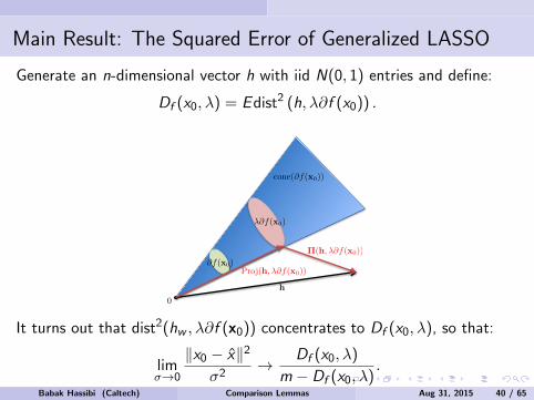

Main Result
limσ→0
‖x0 − x‖2
σ2→ Df (x0, λ)
m − Df (x0, λ).
Note that, compared to the normalized mean-square error of standardleast-squares, n
m−n , the ambient dimension n has been replaced byDf (x0, λ).
The value of λ that minimizes the mean-square error is given by
λ∗ = arg minλ≥0
Df (x0, λ).
It is easy to see that
Df (x0, λ∗) = Edist2 (h, cone(∂f (x0)))
∆= ω2.
Babak Hassibi (Caltech) Comparison Lemmas Aug 31, 2015 41 / 65

Main Result
ω2 = Edist2 (h, cone(∂f (x0)))
The quantity ω2 is the squared Gaussian width of the cone of thesubgradient and has been referred to as the statistical dimension byTropp et al.
Thus, for the optimum choice of λ:
limσ→0
‖x0 − x‖2
‖z‖2→ ω2
m − ω2.
The quantity ω2 determines the minimum number of measurementsrequired to recover a k-sparse signal using (appropriate) convexoptimization. (The so-called recovery thresholds.)
Babak Hassibi (Caltech) Comparison Lemmas Aug 31, 2015 42 / 65

Statistical Dimension
The quantity Df (x0, λ) is easy to numerically compute and ω2 canoften be computed in closed form.
For n-dimensional k-sparse signals and f (x) = ‖x‖1:
ω2 = 2k log2n
k, lim
σ→0
‖x0 − x‖2
‖z‖2→
2k log 2nk
m − 2k log 2nk
For n × n rank r matrices and F (X ) = ‖X‖?:
ω2 = 3r(2n − r) , limσ→0
‖x0 − x‖2
‖z‖2→ 3r(2n − r)
m − 3r(2n − r)
for qb-dimensional k block-sparse signals and f (x) = ‖x‖1,2:
ω2 = 4k(b + logq
k) , lim
σ→0
‖x0 − x‖2
‖z‖2→
4k(b + log qk )
m − 4k(b + log qk )
Babak Hassibi (Caltech) Comparison Lemmas Aug 31, 2015 43 / 65
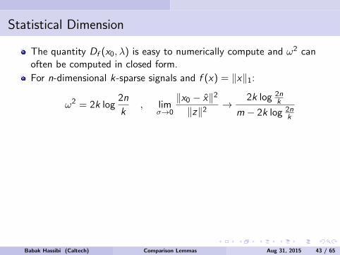
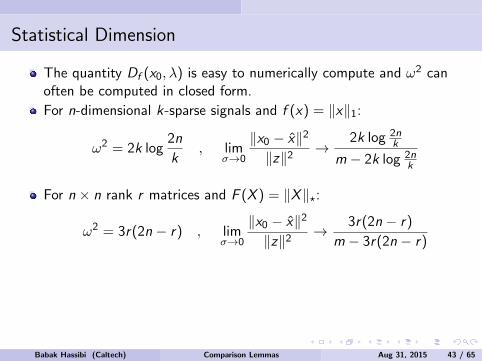
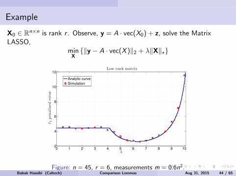
Example
X0 ∈ Rn×n is rank r . Observe, y = A · vec(X0) + z, solve the MatrixLASSO,
minX‖y − A · vec(X )‖2 + λ‖X‖?
0 1 2 3 4 5 6 7 8 9 102
4
6
8
10
12Low rank matrix
λ
ℓ 2pen
alize
der
ror
Analytic curve
Simulation
Figure: n = 45, r = 6, measurements m = 0.6n2.Babak Hassibi (Caltech) Comparison Lemmas Aug 31, 2015 44 / 65
Tuning the Regularizer λ
The optimal value of λ is given by
λ∗ = arg minλ≥0
Df (x0, λ),
which requires knowledge of the sparsity of x0, say.
This is usually notavailable.Question: How to tune λ?Answer: Here is one possibility that uses the fact thatφ(g , h) ≈ σ
√m − Df (x0, λ):
1 Choose a λ and solve the l1 LASSO.2 Find the numerical value of the optimal cost, C , say.3 Find the sparsity k such that
|C − σ√m − Df (x0, λ)|,
is minimized.4 For this value of k find the optimal λ∗.
Babak Hassibi (Caltech) Comparison Lemmas Aug 31, 2015 45 / 65

Tuning the Regularizer λ
The optimal value of λ is given by
λ∗ = arg minλ≥0
Df (x0, λ),
which requires knowledge of the sparsity of x0, say. This is usually notavailable.
Question: How to tune λ?Answer: Here is one possibility that uses the fact thatφ(g , h) ≈ σ
√m − Df (x0, λ):
1 Choose a λ and solve the l1 LASSO.2 Find the numerical value of the optimal cost, C , say.3 Find the sparsity k such that
|C − σ√m − Df (x0, λ)|,
is minimized.4 For this value of k find the optimal λ∗.
Babak Hassibi (Caltech) Comparison Lemmas Aug 31, 2015 45 / 65
Tuning the Regularizer λ
The optimal value of λ is given by
λ∗ = arg minλ≥0
Df (x0, λ),
which requires knowledge of the sparsity of x0, say. This is usually notavailable.Question: How to tune λ?
Answer: Here is one possibility that uses the fact thatφ(g , h) ≈ σ
√m − Df (x0, λ):
1 Choose a λ and solve the l1 LASSO.2 Find the numerical value of the optimal cost, C , say.3 Find the sparsity k such that
|C − σ√m − Df (x0, λ)|,
is minimized.4 For this value of k find the optimal λ∗.
Babak Hassibi (Caltech) Comparison Lemmas Aug 31, 2015 45 / 65

Tuning the Regularizer λ
The optimal value of λ is given by
λ∗ = arg minλ≥0
Df (x0, λ),
which requires knowledge of the sparsity of x0, say. This is usually notavailable.Question: How to tune λ?Answer: Here is one possibility that uses the fact thatφ(g , h) ≈ σ
√m − Df (x0, λ):
1 Choose a λ and solve the l1 LASSO.
2 Find the numerical value of the optimal cost, C , say.3 Find the sparsity k such that
|C − σ√m − Df (x0, λ)|,
is minimized.4 For this value of k find the optimal λ∗.
Babak Hassibi (Caltech) Comparison Lemmas Aug 31, 2015 45 / 65

Tuning the Regularizer λ
The optimal value of λ is given by
λ∗ = arg minλ≥0
Df (x0, λ),
which requires knowledge of the sparsity of x0, say. This is usually notavailable.Question: How to tune λ?Answer: Here is one possibility that uses the fact thatφ(g , h) ≈ σ
√m − Df (x0, λ):
1 Choose a λ and solve the l1 LASSO.2 Find the numerical value of the optimal cost, C , say.
3 Find the sparsity k such that
|C − σ√m − Df (x0, λ)|,
is minimized.4 For this value of k find the optimal λ∗.
Babak Hassibi (Caltech) Comparison Lemmas Aug 31, 2015 45 / 65

Tuning the Regularizer λ
The optimal value of λ is given by
λ∗ = arg minλ≥0
Df (x0, λ),
which requires knowledge of the sparsity of x0, say. This is usually notavailable.Question: How to tune λ?Answer: Here is one possibility that uses the fact thatφ(g , h) ≈ σ
√m − Df (x0, λ):
1 Choose a λ and solve the l1 LASSO.2 Find the numerical value of the optimal cost, C , say.3 Find the sparsity k such that
|C − σ√m − Df (x0, λ)|,
is minimized.
4 For this value of k find the optimal λ∗.
Babak Hassibi (Caltech) Comparison Lemmas Aug 31, 2015 45 / 65

Tuning the Regularizer λ
The optimal value of λ is given by
λ∗ = arg minλ≥0
Df (x0, λ),
which requires knowledge of the sparsity of x0, say. This is usually notavailable.Question: How to tune λ?Answer: Here is one possibility that uses the fact thatφ(g , h) ≈ σ
√m − Df (x0, λ):
1 Choose a λ and solve the l1 LASSO.2 Find the numerical value of the optimal cost, C , say.3 Find the sparsity k such that
|C − σ√m − Df (x0, λ)|,
is minimized.4 For this value of k find the optimal λ∗.Babak Hassibi (Caltech) Comparison Lemmas Aug 31, 2015 45 / 65
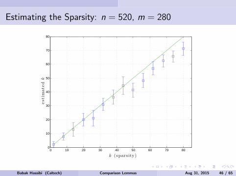
Estimating the Sparsity: n = 520, m = 280
0 10 20 30 40 50 60 70 800
10
20
30
40
50
60
70
80
estim
ate
dk
k (sparsity)
Babak Hassibi (Caltech) Comparison Lemmas Aug 31, 2015 46 / 65

Tuning λ: n = 520, m = 280
0 10 20 30 40 50 60 70 80 900.8
1
1.2
1.4
1.6
1.8
2
2.2
2.4
2.6
k (sparsity)
λbest/√
m
λ
0
theory
Babak Hassibi (Caltech) Comparison Lemmas Aug 31, 2015 47 / 65

Improvement in NSE: n = 520, m = 280
0 10 20 30 40 50 60 70 80 90−10
0
10
20
30
40
50
60
70
80
NSE
i−N
SE
f
NSE
i×
100%
k (sparsity)
Babak Hassibi (Caltech) Comparison Lemmas Aug 31, 2015 48 / 65

Generalizations
Babak Hassibi (Caltech) Comparison Lemmas Aug 31, 2015 49 / 65
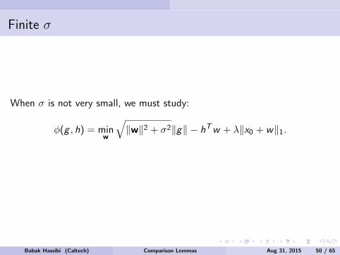
Finite σ
When σ is not very small, we must study:
φ(g , h) = minw
√‖w‖2 + σ2‖g‖ − hTw + λ‖x0 + w‖1.
The analysis is a bit more complicated, but absolutely do-able.
Babak Hassibi (Caltech) Comparison Lemmas Aug 31, 2015 50 / 65

Finite σ
When σ is not very small, we must study:
φ(g , h) = minw
√‖w‖2 + σ2‖g‖ − hTw + λ‖x0 + w‖1.
The analysis is a bit more complicated, but absolutely do-able.
Babak Hassibi (Caltech) Comparison Lemmas Aug 31, 2015 50 / 65
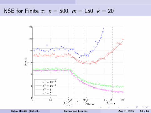
NSE for Finite σ: n = 500, m = 150, k = 20
0 0.5 1 1.5 2 2.50
5
10
15
20
25
30!x
!x
0! 2
!
"
! 2 = 10!4
! 2 = 10!2
! 2 = 1! 2 = 5
λ0crit
λbest λmax
Babak Hassibi (Caltech) Comparison Lemmas Aug 31, 2015 51 / 65

Cost for Finite σ: n = 500, m = 150, k = 20
0 0.5 1 1.5 2 2.50
2
4
6
8
10
12
!!1! !y
!Ax! 2
+" "m(!
x! 1
!!x
0! 1)"
"
! 2 = 10!4
! 2 = 10!2
! 2 = 1! 2 = 5
λ0crit
λbest λmax
Babak Hassibi (Caltech) Comparison Lemmas Aug 31, 2015 52 / 65

Other Loss Functions
We can do other loss functions.
For example,
x = arg minx‖y − Ax‖1 + λ‖x‖,
which attempts to find a sparse signal in sparse noise and which iscalled least absolute deviations (LAD).
In turns out that we now must analyze
φ(g , h) = minw
max‖v‖∞≤1
√‖w‖2 + σ2gTv − ‖v‖hTw + sup
s∈λ∂f (x0)sTw
This is a bit more complicated, but still completely doable.
Babak Hassibi (Caltech) Comparison Lemmas Aug 31, 2015 53 / 65

Other Loss Functions
We can do other loss functions. For example,
x = arg minx‖y − Ax‖1 + λ‖x‖,
which attempts to find a sparse signal in sparse noise and which iscalled least absolute deviations (LAD).
In turns out that we now must analyze
φ(g , h) = minw
max‖v‖∞≤1
√‖w‖2 + σ2gTv − ‖v‖hTw + sup
s∈λ∂f (x0)sTw
This is a bit more complicated, but still completely doable.
Babak Hassibi (Caltech) Comparison Lemmas Aug 31, 2015 53 / 65
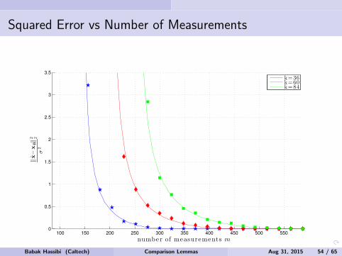
Squared Error vs Number of Measurements
100 150 200 250 300 350 400 450 500 5500
0.5
1
1.5
2
2.5
3
3.5
number of measurements m
‖x−x0‖2 2
σ2
k=36k=60k=84
Babak Hassibi (Caltech) Comparison Lemmas Aug 31, 2015 54 / 65

Squared Error vs Sparsity of Noise
0 0.1 0.2 0.3 0.4 0.5 0.6 0.7 0.8 0.9 10
0.2
0.4
0.6
0.8
1
1.2
1.4
1.6
1.8
2
noise sparsity leve l q
‖x−x0‖2 2
σ2
Average of 25 real i zat i ons
Theorem 3.1
Babak Hassibi (Caltech) Comparison Lemmas Aug 31, 2015 55 / 65

Cost vs Number of Measurements
100 150 200 250 300 350 400 450 500 5500
0.05
0.1
0.15
0.2
0.25
0.3
0.35
0.4
0.45
number of measurements m
‖y−
Ax‖1
k=36
k=60
k=84
Babak Hassibi (Caltech) Comparison Lemmas Aug 31, 2015 56 / 65

Universality
Our results assumed an iid Gaussian A.
Is this necessary?
Simulations suggest that any iid distribution with the same secondorder statistics works.
“Close” to proving this?
Babak Hassibi (Caltech) Comparison Lemmas Aug 31, 2015 57 / 65

Universality
Our results assumed an iid Gaussian A.
Is this necessary?
Simulations suggest that any iid distribution with the same secondorder statistics works.
“Close” to proving this?
Babak Hassibi (Caltech) Comparison Lemmas Aug 31, 2015 57 / 65
Universality
Our results assumed an iid Gaussian A.
Is this necessary?
Simulations suggest that any iid distribution with the same secondorder statistics works.
“Close” to proving this?
Babak Hassibi (Caltech) Comparison Lemmas Aug 31, 2015 57 / 65

Universality
Our results assumed an iid Gaussian A.
Is this necessary?
Simulations suggest that any iid distribution with the same secondorder statistics works.
“Close” to proving this?
Babak Hassibi (Caltech) Comparison Lemmas Aug 31, 2015 57 / 65

NSE for iid Bernouli(12): n = 500, m = 150, k = 20
0 0.5 1 1.5 2 2.50
5
10
15
20
25
30
35
‖x−x
0‖2
σ
λ
σ2= 10
−4
σ2= 10
−2
σ2= 1
σ2= 5
Babak Hassibi (Caltech) Comparison Lemmas Aug 31, 2015 58 / 65

Cost for Bernoulli(12): n = 500, m = 150, k = 20
0 0.5 1 1.5 2 2.50
2
4
6
8
10
12
‖z−A
x‖ 2
+λ √m
(‖x
‖ 1−‖x
0‖ 1
)
σ
λ
σ2 = 10−4
σ2 = 10−2
σ2 = 1
σ2 = 5
Babak Hassibi (Caltech) Comparison Lemmas Aug 31, 2015 59 / 65

Other Matrix Ensembles - Haar
Can we give results for non iid random matrix ensembles?
An important class of random matrices are isotropically randomunitary matrices, i.e., matrices Q ∈ Rm×n (m < n), such that
QQT = Im, P(ΘQΩ) = P(Q),
for all orthogonall Θ and Ω.
For such random matrices, we have shown that the two optimizationproblems:
Φ(Q, z) = minw ‖σz − Qw‖+ λf (w)φ(g , h) = minw ,l maxβ≥0 ‖σv − w − l‖+ β(‖l‖ · ‖g‖ − hT l) + λf (w)
where z , v , h and g have iid N(0, 1) entries, have the same optimalcosts and statistically the same optimal minimizer.
Babak Hassibi (Caltech) Comparison Lemmas Aug 31, 2015 60 / 65

Other Matrix Ensembles - Haar
Can we give results for non iid random matrix ensembles?
An important class of random matrices are isotropically randomunitary matrices,
i.e., matrices Q ∈ Rm×n (m < n), such that
QQT = Im, P(ΘQΩ) = P(Q),
for all orthogonall Θ and Ω.
For such random matrices, we have shown that the two optimizationproblems:
Φ(Q, z) = minw ‖σz − Qw‖+ λf (w)φ(g , h) = minw ,l maxβ≥0 ‖σv − w − l‖+ β(‖l‖ · ‖g‖ − hT l) + λf (w)
where z , v , h and g have iid N(0, 1) entries, have the same optimalcosts and statistically the same optimal minimizer.
Babak Hassibi (Caltech) Comparison Lemmas Aug 31, 2015 60 / 65
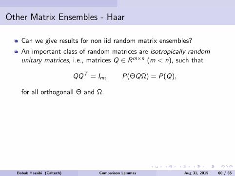
Other Matrix Ensembles - Haar
Can we give results for non iid random matrix ensembles?
An important class of random matrices are isotropically randomunitary matrices, i.e., matrices Q ∈ Rm×n (m < n), such that
QQT = Im, P(ΘQΩ) = P(Q),
for all orthogonall Θ and Ω.
For such random matrices, we have shown that the two optimizationproblems:
Φ(Q, z) = minw ‖σz − Qw‖+ λf (w)φ(g , h) = minw ,l maxβ≥0 ‖σv − w − l‖+ β(‖l‖ · ‖g‖ − hT l) + λf (w)
where z , v , h and g have iid N(0, 1) entries, have the same optimalcosts and statistically the same optimal minimizer.
Babak Hassibi (Caltech) Comparison Lemmas Aug 31, 2015 60 / 65

Other Matrix Ensembles - Haar
Can we give results for non iid random matrix ensembles?
An important class of random matrices are isotropically randomunitary matrices, i.e., matrices Q ∈ Rm×n (m < n), such that
QQT = Im, P(ΘQΩ) = P(Q),
for all orthogonall Θ and Ω.
For such random matrices, we have shown that the two optimizationproblems:
Φ(Q, z) = minw ‖σz − Qw‖+ λf (w)φ(g , h) = minw ,l maxβ≥0 ‖σv − w − l‖+ β(‖l‖ · ‖g‖ − hT l) + λf (w)
where z , v , h and g have iid N(0, 1) entries, have the same optimalcosts and statistically the same optimal minimizer.
Babak Hassibi (Caltech) Comparison Lemmas Aug 31, 2015 60 / 65
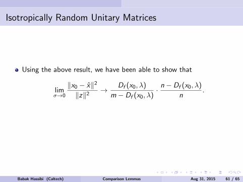
Isotropically Random Unitary Matrices
Using the above result, we have been able to show that
limσ→0
‖x0 − x‖2
‖z‖2→ Df (x0, λ)
m − Df (x0, λ)· n − Df (x0, λ)
n.
Since n−Df (x0,λ)n < 1, this is strictly better than the Gaussian case.
Babak Hassibi (Caltech) Comparison Lemmas Aug 31, 2015 61 / 65

Isotropically Random Unitary Matrices
Using the above result, we have been able to show that
limσ→0
‖x0 − x‖2
‖z‖2→ Df (x0, λ)
m − Df (x0, λ)· n − Df (x0, λ)
n.
Since n−Df (x0,λ)n < 1, this is strictly better than the Gaussian case.
Babak Hassibi (Caltech) Comparison Lemmas Aug 31, 2015 61 / 65
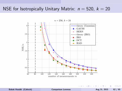
NSE for Isotropically Unitary Matrix: n = 520, k = 20
number of measurements m60 80 100 120 140 160 180 200 220 240
NSE=n
0.5
1
1.5
2
2.5
3
n = 256, k = 24
theory (Gaussian)GAUSSBERNtheory (IRO)IRODCTHAD
Babak Hassibi (Caltech) Comparison Lemmas Aug 31, 2015 62 / 65

Cost for Isotropically Unitary Matrix: n = 520, k = 20
0 50 100 150 200 250 300 350 400 450 5000
50
100
150
200
250
300
350
400
450
m
‖y−Qx‖2
σ2
σ2=10
−4
theory
Babak Hassibi (Caltech) Comparison Lemmas Aug 31, 2015 63 / 65

Other Measurements: Quadratic Gaussians
In certain applications, such as graphical LASSO and phase retrieval, weencounter problems of the following form:
minS≥0
traceGTSG + Ψ(S), (0.1)
where S = ST ∈ Rm×m and G ∈ Rm×n has iid N(0, 1) entries.
Forexample, in graphical LASSO we have
minS≥0
traceGTSG − N log detS + λ‖S‖1.
Problem (0.1) can be linearized as:
minS≥0
maxU
2traceUTSG − traceUTSU + Ψ(S).
Can we come up with comparison lemmas for the Gaussian processtraceUTSG?
Babak Hassibi (Caltech) Comparison Lemmas Aug 31, 2015 64 / 65

Other Measurements: Quadratic Gaussians
In certain applications, such as graphical LASSO and phase retrieval, weencounter problems of the following form:
minS≥0
traceGTSG + Ψ(S), (0.1)
where S = ST ∈ Rm×m and G ∈ Rm×n has iid N(0, 1) entries. Forexample, in graphical LASSO we have
minS≥0
traceGTSG − N log detS + λ‖S‖1.
Problem (0.1) can be linearized as:
minS≥0
maxU
2traceUTSG − traceUTSU + Ψ(S).
Can we come up with comparison lemmas for the Gaussian processtraceUTSG?
Babak Hassibi (Caltech) Comparison Lemmas Aug 31, 2015 64 / 65
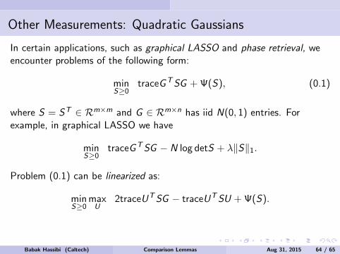
Other Measurements: Quadratic Gaussians
In certain applications, such as graphical LASSO and phase retrieval, weencounter problems of the following form:
minS≥0
traceGTSG + Ψ(S), (0.1)
where S = ST ∈ Rm×m and G ∈ Rm×n has iid N(0, 1) entries. Forexample, in graphical LASSO we have
minS≥0
traceGTSG − N log detS + λ‖S‖1.
Problem (0.1) can be linearized as:
minS≥0
maxU
2traceUTSG − traceUTSU + Ψ(S).
Can we come up with comparison lemmas for the Gaussian processtraceUTSG?
Babak Hassibi (Caltech) Comparison Lemmas Aug 31, 2015 64 / 65
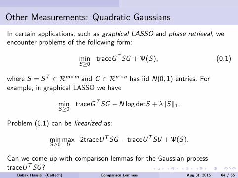
Other Measurements: Quadratic Gaussians
In certain applications, such as graphical LASSO and phase retrieval, weencounter problems of the following form:
minS≥0
traceGTSG + Ψ(S), (0.1)
where S = ST ∈ Rm×m and G ∈ Rm×n has iid N(0, 1) entries. Forexample, in graphical LASSO we have
minS≥0
traceGTSG − N log detS + λ‖S‖1.
Problem (0.1) can be linearized as:
minS≥0
maxU
2traceUTSG − traceUTSU + Ψ(S).
Can we come up with comparison lemmas for the Gaussian processtraceUTSG?
Babak Hassibi (Caltech) Comparison Lemmas Aug 31, 2015 64 / 65
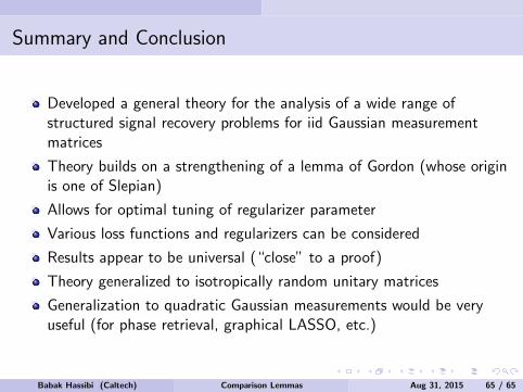
Summary and Conclusion
Developed a general theory for the analysis of a wide range ofstructured signal recovery problems for iid Gaussian measurementmatrices
Theory builds on a strengthening of a lemma of Gordon (whose originis one of Slepian)
Allows for optimal tuning of regularizer parameter
Various loss functions and regularizers can be considered
Results appear to be universal (“close” to a proof)
Theory generalized to isotropically random unitary matrices
Generalization to quadratic Gaussian measurements would be veryuseful (for phase retrieval, graphical LASSO, etc.)
Babak Hassibi (Caltech) Comparison Lemmas Aug 31, 2015 65 / 65


![Compressive Structured Light for Recovering Inhomogeneous ... · Structured light has a long history in the computer vision community [Salvi et al., 2004]. It has matured into a robust](https://static.fdocuments.us/doc/165x107/5f9adf57156b4b62ed3955d9/compressive-structured-light-for-recovering-inhomogeneous-structured-light-has.jpg)