RECONSTRUCTING HOLOCENE SEA-LEVEL CHANGE FOR THE CENTRAL GREATBARRIER REEF (AUSTRALIA) USING SUBTIDAL FORAMINIFERA

BENJAMIN P. HORTON1,8, STEPHEN J. CULVER

2, MICHAEL I. J. HARDBATTLE3, PIERS LARCOMBE

4, GLENN A. MILNE5,

CATERINA MORIGI6, JOHN E. WHITTAKER

7AND SARAH A. WOODROFFE

3

ABSTRACT

We assessed the utility of subtidal foraminifera toreconstruct Holocene relative sea levels from the centralGreat Barrier Reef shelf, Australia. We collected contempo-rary foraminiferal samples from Cleveland Bay and BowlingGreen Bay, with water depths from 24.2 m to 248.0 mAustralian Height Datum (AHD). The subtidal foraminiferalassemblages were divided into two distinct foraminiferalzones: an inner shelf zone occupied by Elphidium hispidulum,Pararotalia venusta, Planispirinella exigua, Quinqueloculinavenusta and Triloculina oblonga; and a middle shelf zonedominated by Amphistegina lessonii, Dendritina striata andOperculina complanata. The zonations of the study areas andrelative abundances of individual species indicate that thedistributions of subtidal foraminifera are related to waterdepth.

We used the subtidal data to develop a transfer functioncapable of inferring past water depths of sediment samplesfrom their foraminiferal content. The results indicateda robust performance of the transfer function (r2

jack 5

0.90). We produced ten sea-level index points, which revealedan upward trend of Holocene relative sea level from 28.86 6

4.5 m AHD at 9.3–8.6 cal kyr BP to a mid-Holocene highstand of +1.72 6 3.9 m AHD at 6.9–6.4 cal kyr BP. Sealevel subsequently fell from the highstand to the present-day.The sea-level reconstructions are consistent with geophysicalmodels and previous published data.

INTRODUCTION

The recent transition of the earth system from a glacial toan interglacial state produced a dramatic, global sea-levelresponse. Fairbanks (1989), Chappell and Polach (1991)and Bard and others (1996) created benchmark, late glacial,and early Holocene relative sea-level curves using coral-based sea-level indicators. These suggest that since the LastGlacial Maximum, approximately 50 million cubic kilo-meters of ice melted from the land-based ice sheets

(Lambeck and others, 2002), raising sea level in tectonicallystable regions that are distant from the major glaciationcenters (far-field sites) by ca. 120 m (e.g., Peltier andFairbanks, 2006). This rapid rise in sea level is attributed tothe eustatic contribution, which averaged 10 mm yr21

during the deglaciation but peak rates potentially exceeded50 mm yr21 during ‘‘meltwater pulses’’ at 19 and14.5 cal kyr BP (e.g., Alley and others, 2005). Empirical(e.g., Fairbanks, 1989; Horton and others, 2005a) andmodeling studies (e.g., Lambeck and others, 2002; Milneand others, 2005) suggest a significant reduction in eustaticcontribution during the Holocene, beginning ca. 7 cal kyrago.

Some of the best records of sea-level change in temperateareas have been derived from benthic intertidal forami-niferal assemblages contained in a range of post-glacialsedimentary deposits (e.g., Scott and Medioli, 1978;Gehrels, 1994). Transfer functions have subsequently beendeveloped allowing precise reconstruction of former sealevels using a statistically based relationship betweencontemporary and fossil foraminiferal assemblages (e.g.,Horton, 1999; Gehrels, 2000; Edwards and others, 2004;Patterson and others, 2004; Gehrels and others, 2005;Horton and Edwards, 2006; Boomer and Horton, 2006;Massey and others, 2006; Southall and others, 2006). InAustralia, Horton and others (2003) and Woodroffe andothers (2005) analyzed intertidal foraminiferal distributionsto assess their ability to reconstruct former sea levels frommangrove environments from the Great Barrier Reefcoastline (GBR). Furthermore, Cann and others (2002)used intertidal foraminifera as indicators of estuarine-lagoonal and oceanic influences in Holocene sediments ofthe Murray River, South Australia. A transfer function wasdeveloped but never applied in mangrove environments ofNorthern Queensland, because of problems with forami-niferal preservation (Horton and others, 2003, 2005b;Woodroffe and others, 2005). Woodroffe and others(2005) and Berkeley and others (2006) demonstrated thatforaminiferal preservation within mangrove sediments ofthe GBR coastline is problematic, concurring with theconclusions of Wang and Chappell (2001) and Debenay andothers (2004), who concluded that foraminifera in man-grove environments are dramatically affected by tapho-nomic processes.

In this paper, we explore the utility of using subtidalrather than intertidal foraminifera to reconstruct former sealevels for tropical environments. We define subtidal as allenvironments from the innermost inner shelf to the middleshelf (0–100 m). Yokoyama and others (2000) inferred thetiming of the Last Glacial Maxima from sea-level recon-structions for the Bonaparte Gulf, Western Australia, basedon the classification of sedimentary facies using sub-tidal foraminifera. However, this classification was only

Journal of Foraminiferal Research fora-37-04-06.3d 26/8/07 13:33:25 47

1 Sea Level Research Laboratory, Department of Earth andEnvironmental Science, University of Pennsylvania, Philadelphia, PA19104-6316, USA.

2 Department of Geology, East Carolina University, Greenville,North Carolina 27858, USA.

3 Department of Geography, University of Durham, South Road,Durham, DH1 3LE, UK.

8 Correspondence author. E-mail: bphorton@sas.upenn.edu

4 Centre for Environment, Fisheries and Aquaculture Science,Pakefield Road, Lowestoft, Suffolk, NR33 0HT, UK.

5 Department of Earth Sciences, University of Durham, South Road,Durham, DH1 3LE, UK.

6 Dipartimento di Scienze del Mare, Universita Politecnica delleMarche, Via Brecce Bianche, 60131 Ancona, Italia.

7 Micropaleontology Research, Department of Palaeontology, TheNatural History Museum, London, SW7 5BD, UK.

Journal of Foraminiferal Research, v. 37, no. 4, p. 000–000, October 2007

0

semi-quantitative and had only four zones (open marine,shallow marine, marginal marine and brackish), givinglimited water-depth constraints (Shennan and Milne, 2003;Peltier and Fairbanks, 2006). We present contemporarysubtidal foraminiferal samples and associated environmen-tal information from two embayments along the centralGBR coastline to demonstrate the relationship of benthicforaminiferal assemblages with water depth. We generatea foraminiferal-based, subtidal transfer function to re-construct former sea levels. These reconstructions arecompared with regional geophysical models and publishedsea-level data.

STUDY AREA

Far-field locations such as Australia are particularlyimportant locations for sea-level reconstructions becausethey enable the examination of the timing and abruptness ofreduction in global melting during the Holocene and theeffect of meltwater load on earth rheology. This enablesa better understanding of the integrated melting history ofglobal late Pleistocene ice sheets and the loading responseof materials of the crust. In addition, sea-level variationsthat have occurred throughout the mid to late Holocene infar-field regions give an insight into natural variabilitywithin a climatic system that is similar to the present one.Sea-level research in Australia includes some of the earliestdebates on hydro-isostasy (e.g., Clark and others, 1978)and, more recently, discussions regarding ocean loadingand continental levering (e.g., Belperio and others, 1984;Baker and Haworth, 2000; Cann and others, 2002; Ha-worth and others, 2002; Sloss and others, 2005; Woodroffe,2006). Larcombe and others (1995a) and Larcombe andCarter (1998) compiled an extensive database of Holocenesea-level observations for the GBR using supra-, inter- andsubtidal indicators. The variability of the data caused a widescatter of sea-level index points, with the result that it wasonly possible to generate an envelope of Holocene sea-levelchanges. Studies from the GBR region (e.g., Carter andothers, 1993; Beaman and others, 1994; Larcombe andothers, 1995a; Larcombe and Carter, 1998) have shown thatthe majority (. 70%) of existing sea-level data are subtidalin nature.

Cleveland Bay and Bowling Green Bay are embaymentsin the central GBR shelf region, Queensland, Australia(Fig. 1a). The GBR shelf is 100 km wide in the centralregion, with water depths reaching 80 m (Maxwell, 1968).The central region of the GBR is thought to have beentectonically stable since at least 13 cal kyr BP (Chappelland others, 1982, 1983). There is no evidence for localtectonic movements since 5.5 cal kyr BP, although Chap-pell and others (1982, 1983) suggested there might havebeen minor hydro-isostatic warping and subsidence normalto the coastline across the shelf since 6 cal kyr BP.Differential flexing along the inner shelf has probably beenless than 1 m, similar to the magnitude of the mid-Holocenefall in relative sea level (Beaman and others, 1994). Theapparent lack of tectonic movement in the central GBRindicates that the results of this study will be applicable toother sites in the region.

Cleveland Bay is a 325 km2 embayment located on theeast coast of north Queensland (Fig. 1b), immediatelyoffshore of Townsville. The southern margin of the bay isformed by salt flats containing chenier ridges, where themuddy shoreline and tidal creeks entering into the bay aremangrove-fringed. The western edge of the bay, on themainland, is backed by a flat, sandy coastal plain, whichhas been extensively modified by human activity over thelast 100 years (removal of mangroves and sand dunes;McIntyre, 1996; Hardbattle, 2003). Separating ClevelandBay from Halifax Bay to the west is Magnetic Island. Thenorthern edge of Cleveland Bay is delineated arbitrarily bythe 20 m isobath, which is also the outer edge of the innershelf (Belperio, 1983; Carter and others, 1993), which isdominated by terrigenous sediments (Maxwell, 1968;Belperio, 1983; Johnson and others, 1986). The easternedge of the bay is bound by a granite headland, whichforms Cape Cleveland. Bowling Green Bay is the larger ofthe two embayments, around 600 km2, and is located 30 kmsoutheast of Cleveland Bay (Fig. 1c). The sand spit of CapeBowling Green protects the eastern side of the bay from theprevailing southeasterly waves. In the south is a broadcoastal plain containing tidal mudflats, mangrove creeksystems and salt marshes. Driven by strong northwardalongshore flows, Bowling Green Bay receives a significantproportion of the 3–20 Mt/y of suspended sedimentsupplied to the coast by the Burdekin River, which entersthe lagoon immediately south of Cape Bowling Green(Belperio, 1979; Neil and others, 2002; Orpin and others,2004). Within the Bowling Green Bay, the coastal plains arecrossed by the Haughton River, which flows five to sixmonths of the year and supplies sandy terrigenous sedimentto the nearshore.

METHODOLOGY

Contemporary and fossil samples from Cleveland Bayand Bowling Green Bay were collected by researchers fromJames Cook University, Australia and the AustralianInstitute of Marine Science. The samples were collectedon cruise numbers KG857, KG902, KG911 and KG912baboard R/V James Kirby. We selected forty-three 10-cm3

samples of surface sediment and ten vibracores fromsubtidal locations from transects within Cleveland Bayand Bowling Green Bay for foraminiferal and lithologicalanalyses (Fig. 1). Details of the chronology and lithofaciesof the vibracores have been published by Larcombe andothers (1995a), McIntyre (1996) and Larcombe and Carter(1998). We selected one dated sample from each vibracorefor foraminiferal analyses (Table 1). The lithology of allsamples indicated they were analogous to the subtidalenvironments of Cleveland Bay and Bowling Green Bay(Belperio, 1979, 1983; Carter and others, 1993; McIntyre,1996; Larcombe and Carter, 1998; Orpin and others, 2004),thus improving the likelihood of reliable sea-level recon-structions. Furthermore, the selected radiocarbon datesrange from the early Holocene to present. We calibrated theradiocarbon data using OxCal (ver 3.10; Bronk Ramsey,2005) and the marine04.14c dataset, where appropriate(Hughen and others, 2004). The resulting sequence of ages

Journal of Foraminiferal Research fora-37-04-06.3d 26/8/07 13:33:55 48

0 HORTON AND OTHERS

was used to constrain the variations in sea level identifiedfrom the subtidal foraminiferal data.

The water depths of the contemporary and fossil sampleswere calculated from depth soundings taken at samplingpoints with a 3.5 kHz precision depth recorder (using, ingeneral, a 0.25 s firing rate, 6 kHz bandwidth and 0.5 mspulse length). These readings were corrected for the depthof the transducer below the sea surface, then converted tothe Australian Height Datum (AHD) through using thedate and time of sample collection and tide gauge records atTownsville. The resulting magnitude of the errors isbetween 6 0.3 m and 6 0.5 m (Hardbattle, 2003).

Contemporary and fossil foraminiferal sample preparationfollowed Scott and others (2001). Samples were wet-sievedthrough sieves with 500-mm and 63-mm openings anddecanted using a wet splitter (Scott and Hermelin, 1993).We examined the .500 mm and decanted fractions beforediscarding them. We did not use any floatation techniques,and all the samples were picked wet. We analyzed the totalassemblage. Modern and fossil samples produced forami-niferal counts .250 individuals per sample. The specieswere identified with reference to a number of publications,namely Brady (1884), Bronnimann and Whittaker (1993),Jones (1994), Loeblich and Tappan (1994), Yassini and

Journal of Foraminiferal Research fora-37-04-06.3d 26/8/07 13:33:55 49

FIGURE 1. Location map of the study area showing (a) the Great Barrier Reef coastline Australia, contemporary sites of (b) Cleveland Bay and (c)Bowling Green Bay and (d) vibracore sites of Cleveland Bay. The samples were collected on cruise numbers KG857, KG902, KG911 and KG912baboard R/V James Kirby.

SUBTIDAL FORAMINIFERA 0

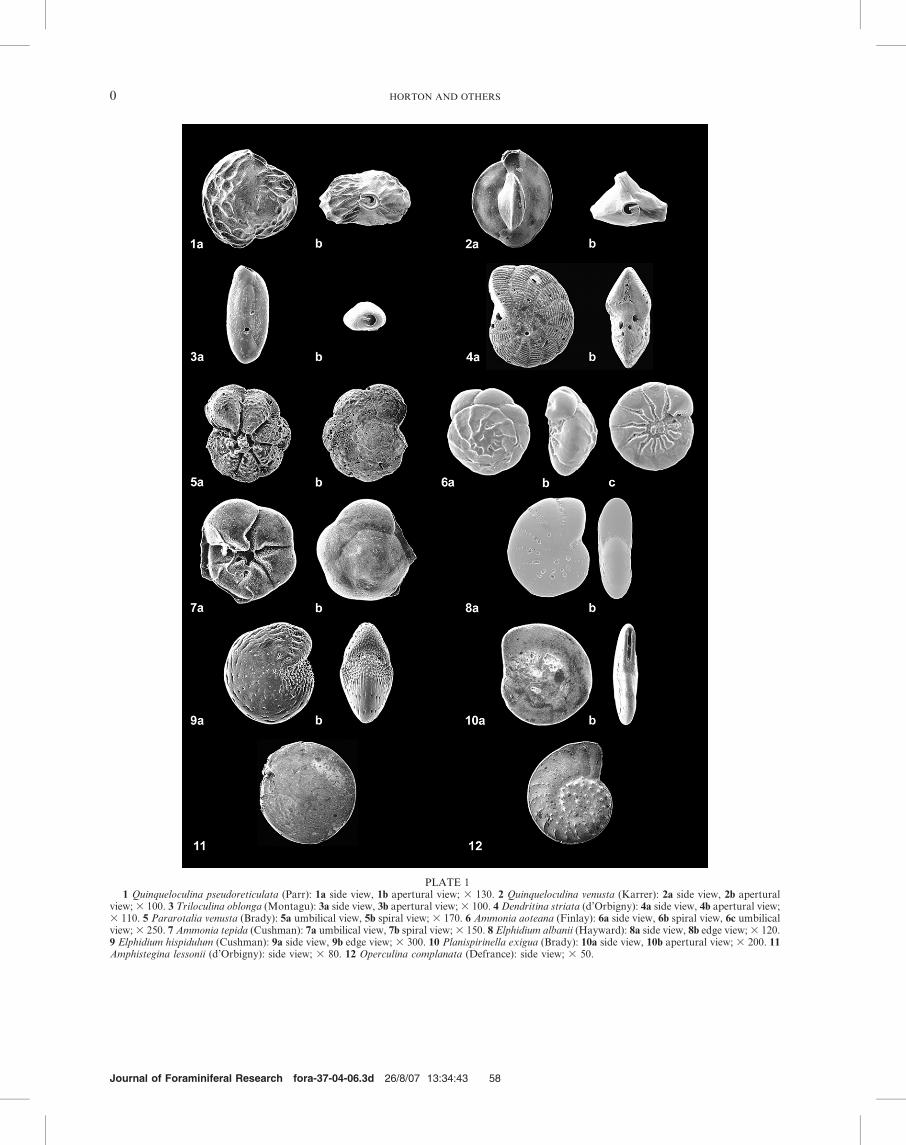
Jones (1995) and Hayward and others (1997, 1999), and bystudy of reference collections in the Natural HistoryMuseum, London (Plate 1).

We used two multivariate methods to detect, describeand classify patterns within the contemporary foraminiferaldataset. Unconstrained cluster analysis, based on theunweighted Euclidean distance with no transformation orstandardization of the percentage data and amalgamationusing the incremental sum of squares within each group(Grimm, 2004), was used to classify contemporary samplesinto more-or-less homogeneous faunal zones (clusters). Weused unconstrained cluster analysis because it comparessamples without any stratigraphic constraint. Detrendedcorrespondence analysis (DCA), an ordination technique,was used to represent samples as points in multi-dimen-sional space, where similar samples plot close together anddissimilar samples apart (ter Braak and Smilauer, 1997–2003). Thus, cluster analysis is effective in classifying thesamples according to their foraminiferal assemblage. DCAgives further information about the pattern of variationwithin and between groups and is important because theprecise boundaries between clusters can be arbitrary (Birks,1986; 1992). Thus, our selection of foraminiferal zones wasbased on whether the samples within each cluster weremutually exclusive in ordination space. The water depth ofeach station within the clusters determined the bathymetricdistribution of each delineated subtidal environment.

We determined the grain size distribution using a Beck-man Coulter laser particle-size analyzer, following thesediment preparation procedures of Goff and others(2004) and Hawkes and others (in press). Organic contentof the sediments was determined by loss on ignition (LOI),following the procedures of Ball (1964).

RESULTS

CLEVELAND BAY

The two transects in Cleveland Bay were 8 km and 4 kmin length and covered water depths from 24.2 m to 29.8 mAHD. The Cleveland Bay seabed was a silty sand with loworganic content (,5%). The sand content increased sea-ward from 44% at a water depth of 25.6 m AHD to 98% at27.4 m AHD. We identified twenty-six foraminiferal

species from the eighteen sampling stations of the twotransects at Cleveland Bay. The assemblages of the twotransects were dominated by five species (Elphidiumhispidulum, Pararotalia venusta, Planispirinella exigua,Quinqueloculina venusta and Triloculina oblonga; Fig. 2).The landward section of Transect 1 was dominated by E.hispidulum, with notable contributions from T. oblonga.The maximum relative abundance of both these species(30% and 12%, respectively) occurred at 2.9 km along thetransect, with a water depth of 25.5 m AHD. These specieswere replaced by Q. venusta and P. exigua at deeper waterdepths. The maximum relative abundance of Q. venusta(16%) occurred at 6 km along the transect in a water depthof 26.0 m AHD, whereas P. exigua peaked (24%) at theseaward end of the transect, with a water depth of 29.8 mAHD.

The landward edge of Transect 2 was dominated byElphidium hispidulum and Pararotalia venusta. Their max-imum relative abundances (23% and 24%, respectively)occurred at a water depth of 24.2 m AHD. These specieswere replaced by Quinqueloculina venusta and Planispir-inella exigua. The relative abundance of Q. venustaexceeded 30% at 2.2 km along the transect, with a waterdepth of 27.9 m AHD. The seaward edge of the transecthad the maximum relative abundance of Quinqueloculinapseudoreticulata (17% at a water depth of 26.0 m AHD).

Multivariate analyses of a combined dataset of transects1 and 2 identified two foraminiferal zones (Fig. 3). ZoneCB-I was dominated by Amphistegina lessonii, Pararotaliavenusta, Quinqueloculina venusta and Q. pseudoreticulata.This zone had a water depth range of 24.2 m to 27.9 mAHD. Zone CB-II was occupied by Elphidium hispidulum,Haynesina depressula and Planispirinella exigua, the latterof which exceeded 10% in all samples. This zone had a waterdepth range of 25.5 m to 29.8 m AHD.

BOWLING GREEN BAY

The Bowling Green Bay transect was much longer(65 km) than that of the Cleveland Bay and extended froma depth of 26.7 m AHD through the inner and middleshelves of the GBR lagoon to a depth of 248.0 m AHD.The substrate of the Bowling Green Bay transect was a siltysand, with a low clay (# 13%) and organic matter (, 8%)

Journal of Foraminiferal Research fora-37-04-06.3d 26/8/07 13:34:10 50

Table 1. Sea-level index points from Cleveland Bay collected on cruise numbers KG857, KG902, KG911 and KG912b aboard R/V James Kirby. Allmean 14C 6 1s dates are calibrated using OxCal (ver 3.10; Bronk Ramsey, 2005) and 2s. * We have used the marine04.14c dataset (Hughen andothers, 2004) and DR of 219 6 38 years (Ulm, 2002). The water depth is predicted using the subtidal transfer function. Relative sea level (RSL) iscalculated from the combination of elevation (m AHD) and water depth. The RSL error calculation includes the sum of all the quantified, orestimated, height errors; these include transfer function error, sample elevation error and sample thickness [total error 5 !(e1

2 + e22 + . . ..en

2 )].

Sample Dated material Laboratory code 14C age BP (61s) Calibrated age range RSL (m AHD)

911v15* Marginopora GAK2211 2100 6 164 2098–1326 20.6 6 4.4902v102* Bursa rana GAK2453 2270 6 144 2283–1560 20.3 6 3.7902v121* Vexillium amanda GAK2449 2860 6 213 3183–2096 0.6 6 3.9911v16* Ostrea sp. GAK2215 4200 6 78 4551–4064 0.9 6 3.9911v8* Bivalves GAK2443 6153 6 95 6863–6379 1.7 6 3.9857dv16 Plant macro GAK7224 6310 6 170 7600–6750 1.7 6 3.8912bv4* Austromactra dissimillis GAK2444 7741 6 97 8413–7993 22.9 6 3.8902v113 Organic mud GAK3553 7840 6 170 9150–8300 25.6 6 4.3902v106 Organic mud GAK3550 8110 6 210 9550–8500 25.8 6 4.1911v11* Gastropod GAK2210 8380 6 125 9330–8598 28.9 6 4.5

0 HORTON AND OTHERS

content. The percentage of silt decreased with increasingwater depth from 22% at 210.1 m AHD to 4.2% at248.0 m AHD. We identified thirty-one species fromtwenty-five stations along the Bowling Green Bay transect.The assemblage was dominated by five species (Fig. 4).Elphidium hispidulum, Planispirinella exigua and Quinque-loculina venusta dominated the inner shelf. Indeed, allspecies had their maximum abundances within the innershelf; E. hispidulum (19%), P. exigua (16%) and Q. venusta(17%) peaked at 4.5 km, 10 km and 4.5 km along thetransect, respectively, within shallow water depths(.213 m AHD). The proportion of these three speciesdecreased at the transition with the middle shelf, to be

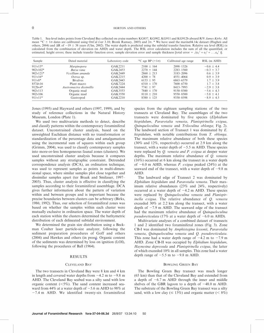
replaced by Amphistegina lessonii and Dendritina striata.High relative abundances of D. striata were restricted to thelandward section of the middle shelf, with its maximumabundance (23%) occurring at 27.5 km along the transect,with a water depth of 225 m AHD. A. lessonii dominatedthe seaward section of the middle shelf with a maximumabundance of 41% at 52 km along the transect with a waterdepth of 238.5 m AHD. Multivariate analysis clearlyidentified two zones (Fig. 5). Zone BGB-I comprised 12sites and was dominated by E. hispidulum, P. exigua and Q.venusta, with a virtual absence of A. lessonii, D. striata andOperculina complanata. The zone occurred at water depthsof 26.7 m to 217.0 m AHD. In contrast, Zone BGB-II

Journal of Foraminiferal Research fora-37-04-06.3d 26/8/07 13:34:10 51

FIGURE 2. Relative foraminiferal abundance (%) of the five most abundant foraminiferal species from Cleveland Bay (a) Transect 1 and (b)Transect 2. Water depth and distance along the transect (km) are indicated.

SUBTIDAL FORAMINIFERA 0

encompassed thirteen sites where A. lessonii, D. striata andO. complanata were dominant. The relative abundance ofA. lessonii exceeded 20% in ten of the thirteen samples. Thezone included water depths from 218.5 to 248.0 m AHD.

TRANSFER FUNCTION DEVELOPMENT

We combined the subtidal foraminifera from ClevelandBay and Bowling Green Bay into one modern dataset toincrease the range of environments to ensure that mostfossil samples have a modern analogue. This will introduceinherent noise into the data set because Cleveland Bay and

Bowling Green Bay have different physiographic condi-tions. Nevertheless, DCA of the combined dataset showedconsiderable overlap between sites (Fig. 6). We developeda transfer function using a unimodal-based techniqueknown as weighted averaging partial least squares (WA-PLS; Juggins, 2004). The dataset consisted of thirty-onespecies and forty-three samples. We did not screen anysamples or species from the dataset. The WA-PLS transferfunction produced results for five components. The choiceof component depended upon the prediction statistics: root-mean square of the error of prediction (RMSEP) and thesquared correlation (r2) of observed versus predicted values.

Journal of Foraminiferal Research fora-37-04-06.3d 26/8/07 13:34:16 52

FIGURE 3. (a) Unconstrained cluster analysis based on unweighted Euclidean distances showing the contemporary foraminiferal assemblagesversus order of samples on dendrogram, (b) detrended correspondence analysis (sample label is shown) and (c) bathymetric distribution of ClevelandBay transects 1 and 2. Only species with relative abundances greater than 10% in one or more samples are shown.

0 HORTON AND OTHERS

The RMSEP indicates the systematic differences in pre-diction errors, whereas the r2 measures the strength of therelationship of observed versus predicted values. Thesestatistics were calculated as apparent measures in which thewhole, contemporary dataset was used to generate thetransfer function and assess the predictive ability. The datawere also jack-knifed (also known as ‘‘leave-one-out’’measures; Birks, 1995) to produce a measure of the overallpredictive abilities of the dataset. Jack-knifing is thesimplest approach of cross-validation (ter Braak andJuggins, 1993) where the reconstruction procedure isapplied n times using a modern dataset of size (n – 1). Ineach of the n predictions, one sample is left out in turn, andthe calibration function based on the (n – 1) sites in themodern dataset is applied to the omitted sample, giving

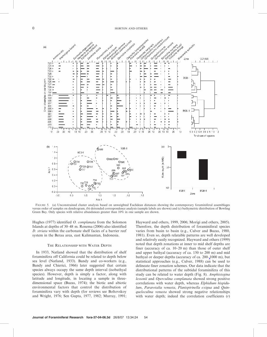
a predicted water depth, which can be subtracted from theobserved water depth to produce a prediction error forthe sample (Birks, 1995). We chose component two for thetransfer function because it performed significantly betterthan component one when jack-knifed errors were consi-dered; prediction errors (RMSEP) were lower, and squaredcorrelations (r2) were higher (Table 2). Using componenttwo, the relationship between observed and subtidalforaminiferal predicted elevation was very strong (Fig. 7),a result that illustrated the robust performance of the WA-PLS transfer function (r2

jack 5 0.90). These results indicatethat reconstructions of former sea levels are possible(RMSEPjack 5 3.50 m).

DISCUSSION

SUBTIDAL FORAMINIFERAL DISTRIBUTION

Our multivariate analysis of the subtidal foraminifera ofCleveland Bay and Bowling Green Bay has identified twoforaminiferal zones. The first zone is dominated byElphidium hispidulum, Pararotalia venusta, Planispirinellaexigua, Quinqueloculina venusta and Triloculina oblonga andoccupied the shallow-water, inner-shelf environment. Sim-ilar subtidal assemblages have been found elsewhere intropical and temperate environments. For example, E.hispidulum has been found in coral-enclosed lagoons, baysand outer reef slopes from the western Pacific (Loeblich andTappan, 1994; Hayward and others, 1997), New SouthWales and Queensland (Albani and Yassini, 1993) and NewCaledonia (Debenay, 1988). P. venusta occurs in the sedi-mentary facies of Exmouth Gulf, northwestern Australia(Orpin and others, 1999a) and Madang Reef and Lagoon,Papua New Guinea (Langer and Lipps, 2004). T. oblongahas been found in normal-marine to hypersaline saltmarshes and lagoonal environments of Georgia and Texas,USA, Bermuda, Tobago and French Guiana, in waterdepths less than 10 m (e.g., Phleger, 1960; Brasier, 1975;Radford, 1976; Goldstein and Frey, 1986; Murray, 1991;Debenay and others, 2001).

The second zone, dominated by Amphistegina lessonii,Dendritina striata and Operculina complanata, occurred inthe middle shelf. This area is between the shore-connectedsediment wedge and the inner edge of the main reef tract atapproximately 40 m. A study of the Gulf of Elat, in the RedSea, suggested that A. lessonii has a depth range toapproximately 90 m below sea level (Hottinger, 1977).Indeed, Hottinger (1977) found the maximum abundance ofthis species at depths of 35–40 m, similar to our findingsalong the Bowling Green Bay transect. Murray (1991)described two A. lessonii associations: firstly, a continentalshelf association from Seto, Japan, and the Banda Sea, witha sandy substrate and water depths of 0–10 m (Uchio, 1962,1967; van Marle, 1988); and secondly, beach and lagoonassociations from numerous tropical islands of the Pacific,with water depths of 0–38 m (Hallock, 1984; Debenay,1985). O. complanata occurred preferentially in sandysubstrates and low light intensities (Hohenegger and others,2000). This species has been found in Bali, Indonesia andJapan (Renema, 2002; Renema and Troelstra, 2001;Renema and others, 2001; Hohenegger and others, 2000).

Journal of Foraminiferal Research fora-37-04-06.3d 26/8/07 13:34:21 53

FIGURE 4. Relative foraminiferal abundance (%) of the six mostabundant foraminiferal species from Bowling Green Bay. Water depthand distance along the transect (m) are indicated.

SUBTIDAL FORAMINIFERA 0

Hughes (1977) identified O. complanata from the SolomonIslands at depths of 30–48 m. Renema (2006) also identifiedD. striata within the carbonate shelf facies of a barrier reefsystem in the Berau area, east Kalimantan, Indonesia.

THE RELATIONSHIP WITH WATER DEPTH

In 1933, Natland showed that the distribution of shelfforaminifera off California could be related to depth belowsea level (Natland, 1933). Bandy and co-workers (e.g.,Bandy and Chierici, 1966) later suggested that certainspecies always occupy the same depth interval (isobathyalspecies). However, depth is simply a factor, along withlatitude and longitude, in locating a sample in three-dimensional space (Buzas, 1974); the biotic and abioticenvironmental factors that control the distribution offoraminifera vary with depth (for reviews see Boltovskoyand Wright, 1976; Sen Gupta, 1977, 1982; Murray, 1991;

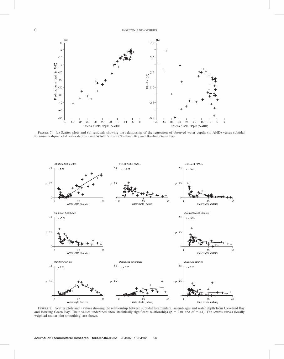
Hayward and others, 1999, 2006; Morigi and others, 2005).Therefore, the depth distribution of foraminiferal speciesvaries from basin to basin (e.g., Culver and Buzas, 1980,1981). Even so, depth relatable patterns are well developedand relatively easily recognized. Hayward and others (1999)noted that depth zonations at inner to mid shelf depths arefiner (accuracy of ca. 10–20 m) than those of outer shelfand upper bathyal (accuracy of ca. 150 to 200 m) and midbathyal or deeper depths (accuracy of ca. 200–1000 m), butstatistical approaches (e.g., Culver, 1988) can be used todelineate finer zonation schemes. Our data indicate that thedistributional patterns of the subtidal foraminifera of thisstudy can be related to water depth (Fig. 8). Amphisteginalessonii and Operculina complanata showed strong positivecorrelations with water depth, whereas Elphidium hispidu-lum, Pararotalia venusta, Planispirinella exigua and Quin-queloculina venusta showed strong negative relationshipswith water depth; indeed the correlation coefficients (r)

Journal of Foraminiferal Research fora-37-04-06.3d 26/8/07 13:34:24 54

FIGURE 5. (a) Unconstrained cluster analysis based on unweighted Euclidean distances showing the contemporary foraminiferal assemblagesversus order of samples on dendrogram, (b) detrended correspondence analysis (sample labels are shown) and (c) bathymetric distribution of BowlingGreen Bay. Only species with relative abundances greater than 10% in one sample are shown.

0 HORTON AND OTHERS

exceed the critical value at p 5 0.01. Dendritina striataillustrated a unimodal relationship with water depth.

RECONSTRUCTION OF FORMER SEA LEVELS

We calibrated the subtidal regional transfer function toten radiocarbon-dated samples from vibracores of Cleve-land Bay (Fig. 1d,). The transfer function assigned a waterdepth to each sample (Table 1). We used bootstrapping toderive a sample-specific root mean squared error ofprediction for individual samples (Birks and others, 1990;Line and others, 1994). Errors are likely to be relativelysmall for fossil assemblages consisting of taxa that arefrequent and abundant in the modern dataset and are likelyto be relatively large for fossil assemblages consisting oftaxa that are infrequent and rare in the modern dataset(Birks, 1995). We also employed the modern analoguetechnique (Juggins, 2004) to evaluate the likely reliability ofwater depth reconstructions based on the subtidal transferfunction. The technique compares numerically, using chi-square distance dissimilarity coefficient, the foraminiferalassemblage in a fossil sample with the foraminiferalassemblages in all available modern samples. Throughusing the largest minimum dissimilarity coefficient (Woo-drofffe, 2006), we illustrated that all fossil samples hada good analogue in the modern dataset. Foraminiferalassemblages of the radiocarbon-dated samples showeda group of species comparable to the contemporaryenvironment (Fig. 9). The lowest sample sum of contem-porary foraminifera in a fossil assemblage was 75%.Samples 911v15, 911v16 and 911v11 were dominated byAmphistegina lessonii with contributions from Dendritinastriata, Operculina complanata and Pararotalia venusta, allof which are indicative of middle shelf environments. Thereconstructed water depths were the deepest of all

radiocarbon-dated samples (,227 m AHD). In contrast,samples 911v18, 902v113 and 902v106 had the shallowestassigned water depth (.29 m AHD). Elphidium albanii wasthe most dominant species in these samples and occurred inthe modern inner shelf environment of Bowling Green Bayand Cleveland Bay. The sample-specific errors for the waterdepth reconstructions varied between 6 3.7 m and 6 4.5 m.These errors are relatively small when compared to the longenvironmental gradient of the dataset (24.2 m AHD to248.0 m AHD); the sample-specific errors are at most 12%

of the vertical range of the dataset. In comparison, some ofthe smallest sample-specific errors (6 0.05 m to 6 0.21 m)were from salt marshes in North Carolina, USA (Hortonand others, 2006). However, these represented 14% of thevertical range of the modern dataset. Furthermore, theerrors are comparable to reconstructions based on corals,which are by far the most widely used sea-level indicators intropical locations (Fairbanks, 1989; Toscano and Macin-tyre, 2003; Peltier and Fairbanks, 2006).

In addition to the sample-specific errors, caution shouldbe exercised when using transfer functions, becausecharacteristics within the contemporary and fossil datamay affect the accuracy of water depth reconstructions.There is an uneven spatial sampling within the contempo-rary data with respect to water depth. Twenty of the forty-three samples were taken in water depths of 24 m to210 m AHD. The transfer function reconstructions aremade from individual water depth measurements for eachdated sample, rather than samples in sequences that couldreveal deepening or shallowing trends. Thus, the recon-struction may be erroneous because of post-depositionalchanges, particularly poor preservation of the calcareoustests, bioturbation and transport of tests from and into anassemblage. The loss of calcareous tests is an importanttaphonomic effect experienced by benthic foraminifera,occurring mainly in regions of high organic carbonconcentrations (e.g., Murray and Alve, 1999). The organiccontent of Bowling Green Bay and Cleveland Bay,however, was less than 8%, suggesting the dissolution ofcalcareous tests is minimal. Bioturbation commonly occursin the top few centimeters of sediments below the sea floorwith slower, more episodic bioturbation below this depth.However, bioturbation can occur at depths greater than12 cm (Aller and Cochran, 1976). The rate varies seasonallyand is highest in summer (Green and others, 1993).Bioturbation is critical in promoting the dissolution ofcalcareous foraminiferal tests as it prevents reactionproduct build-up and stimulates aerobic metabolites, iron

Journal of Foraminiferal Research fora-37-04-06.3d 26/8/07 13:34:29 55

FIGURE 6. Detrended correspondence analysis of the combineddataset from Cleveland Bay and Bowling Green Bay.

Table 2. Apparent errors of estimation and prediction errors forcomponents 1–5 of the WA-PLS subtidal foraminiferal-based transferfunctions. Root-mean square of the error of prediction (RMSEP) andthe squared correlation (r2).

ComponentApparent

(r2)Apparent

RMSE (m)Prediction

(r2)Prediction

RMSEP (m)

1 0.87 3.83 0.83 4.422 0.94 2.50 0.90 3.503 0.96 2.11 0.89 3.644 0.97 1.95 0.87 3.895 0.97 1.76 0.85 4.27

SUBTIDAL FORAMINIFERA 0

Journal of Foraminiferal Research fora-37-04-06.3d 26/8/07 13:34:32 56

FIGURE 7. (a) Scatter plots and (b) residuals showing the relationship of the regression of observed water depths (m AHD) versus subtidalforaminiferal-predicted water depths using WA-PLS from Cleveland Bay and Bowling Green Bay.

FIGURE 8. Scatter plots and r values showing the relationship between subtidal foraminiferal assemblages and water depth from Cleveland Bayand Bowling Green Bay. The r values underlined show statistically significant relationships (p 5 0.01 and df 5 41). The lowess curves (locallyweighted scatter plot smoothing) are shown.

0 HORTON AND OTHERS

sulfide oxidation and nitrification (Green and others, 1993).Conversely, it can result in foraminifera bypassing thedissolution zone, either through biogenic subduction or byfalling into tubes or burrows (Green and others, 1993).Regarding the transport of foraminifera, the headlands ofCape Bowling Green and Cape Cleveland protect theembayments from the dominant southeast waves andalongshore currents, which, in the long-term, transportsediments and foraminiferal tests regionally to the north-west. However, the western side of Bowling Green Bay ismuch more exposed than in the lee of the headland (e.g.,Belperio, 1983).Thus, much of the sediment is resuspended(McIntyre, 1996; Larcombe and Carter, 2004), which maymix the foraminifera. Furthermore, the embayments lieopen to northerly and northeasterly weather and the effectsof tropical cyclones, which are a common seasonal featureof the GBR shelf, typically occurring two to three times persummer at this latitude (Oliver, 1978; Gagan and others,1988, 1990; Massell and Done, 1993; Larcombe and Carter,2004). Despite these processes, our samples lack abraded,etched or broken tests and consist of the full spectrum of testsizes. This is likely to be partly related to the time elapsedsince the last major cyclone-driven flows along the middleshelf (Larcombe and Carter, 2004). Unfortunately, there areno direct methods of detecting erroneous reconstructedreference water depths. Therefore, the most importantindirect method is comparison with other lithostratigraphi-cal, biostratigraphical and modeling techniques.

To further examine the reliability of the transfer functionapproach, we have compared our sea-level reconstructionswith existing geophysical model data and published sea-level data from the study area. Figure 10 shows two sea-level predictions for the GBR coastline based on a com-pressible Maxwell visco-elastic Earth model, which isspherically symmetric and self-gravitating (Horton andothers, 2005a; Milne and others, 2005). The elastic anddensity structure of the model are taken from seismicconstraints (Dziewonski and Anderson, 1981). The viscousstructure is defined in three layers: a very high viscosity

Journal of Foraminiferal Research fora-37-04-06.3d 26/8/07 13:34:39 57

FIGURE 9. Dominant species in Cleveland Bay vibracores. Only species with relative abundances greater than 10% are shown. Water depths (m)predicted using WA-PLS with associated error ranges are shown.

FIGURE 10. Holocene sea-level reconstructions for Cleveland Bayusing the subtidal foraminiferal-based transfer function. Two geo-physical model predictions are shown as dashed lines, whichcorrespond to outer shell (or lithosphere) thicknesses of 120 km and96 km. The sea-level index points show calibrated age ranges and therelative sea-level error (see Table 1).

SUBTIDAL FORAMINIFERA 0

Journal of Foraminiferal Research fora-37-04-06.3d 26/8/07 13:34:43 58

PLATE 11 Quinqueloculina pseudoreticulata (Parr): 1a side view, 1b apertural view; 3 130. 2 Quinqueloculina venusta (Karrer): 2a side view, 2b apertural

view; 3 100. 3 Triloculina oblonga (Montagu): 3a side view, 3b apertural view; 3 100. 4 Dendritina striata (d’Orbigny): 4a side view, 4b apertural view;3 110. 5 Pararotalia venusta (Brady): 5a umbilical view, 5b spiral view; 3 170. 6 Ammonia aoteana (Finlay): 6a side view, 6b spiral view, 6c umbilicalview; 3 250. 7 Ammonia tepida (Cushman): 7a umbilical view, 7b spiral view; 3 150. 8 Elphidium albanii (Hayward): 8a side view, 8b edge view; 3 120.9 Elphidium hispidulum (Cushman): 9a side view, 9b edge view; 3 300. 10 Planispirinella exigua (Brady): 10a side view, 10b apertural view; 3 200. 11Amphistegina lessonii (d’Orbigny): side view; 3 80. 12 Operculina complanata (Defrance): side view; 3 50.

0 HORTON AND OTHERS

outer shell, or lithosphere, with thicknesses of 96 and120 km; a sub-lithosphere upper mantle region witha viscosity of 5 3 1020 Pas to a depth of 670 km; anda lower mantle region with a viscosity of 1022 Pas from670 km to the core-mantle boundary. This viscositystructure is broadly compatible with that inferred ina number of recent studies (e.g., Mitrovica and Forte,1997; Kaufmann and Lambeck, 2002; Milne and others,2005). The ice model adopted to generate the predictionsshown in Figure 10 is based on the ICE-3G deglaciationhistory (Tushingham and Peltier, 1991). A number ofrevisions have been made to the original ICE-3G model.The most significant changes are the addition of a glaciationphase and an increase in the volume and melt chronology ofthe Laurentide component of the model in order to producea good fit to the Barbados sea-level record, based onassuming the reference viscosity model described above.The ice model is characterized by a large decrease in the rateof melt at 7 cal. kyr BP, so the sea-level predictions displaya marked highstand at this time (see Milne and others,2005, for more details).

Sea-level index points were extracted from the transfer-function output by combining the water-depth reconstruc-tions with the elevation of each sediment sample relative toAHD. These index points were then placed in a temporalframework using the chronological data (Table 1). Thegeneral pattern of relative sea-level change indicated by thesubtidal transfer function is consistent with the results ofgeophysical modeling (Fig. 9). Furthermore, in commonwith other far-field regions, the general pattern of relativesea-level change is of an initially rapid rise during the earlyHolocene, from 28.9 6 4.5 m AHD at 9.3–8.6 cal kyr BP.This rise culminated in a middle Holocene highstand of ca.+1.7 6 3.9 m AHD between 7.6–6.4 cal kyr BP, and thena fall to the present. Chappell and others (1983) andBeaman and others (1994) inferred that relative sea levelrose rapidly through the early Holocene, rising above thepresent level at ca. 6.7 cal kyr BP; the amplitude of thehighstand was, however, greater than in this study.Larcombe and others (1995a) and Larcombe and Carter(1998) concluded that the Holocene sea-level highstandoccurred slightly later at ,6.3 cal kyr BP, but with a nearidentical amplitude to the current study (,1.5 m above thepresent level). Beaman and others (1994) used the elevationsof intertidal rock oyster shells on Magnetic Island tosuggest that the mid-Holocene highstand was ca. +1.7 mAHD between 6.5–4.4 cal kyr BP. An interpolation ofChappell and others’ (1982) isobase map predicts thatrelative sea level was 1–2 m above the present level inCleveland Bay at 6.3 cal kyr BP.

This paper indicates that sea-level reconstructions usingsubtidal foraminiferal-based transfer functions can producereliable results. However, the Holocene physiography andenvironmental history of this relatively wide central sectionof the GBR shelf may be favorable to the success of thistechnique; it should not be assumed that this techniquemight be reproducible elsewhere. Specifically, prior to andduring the mid-Holocene highstand, the along-contour,sediment-transport on the GBR shelf (Larcombe andWoolfe, 1999; Gagan and others, 1988, 1990; Larcombeand Carter, 2004) and the resulting strong regional cross-shelf

sedimentary gradients (Maxwell, 1968; Belperio, 1983,1988; Johnson and Searle, 1984; Scoffin and Tudhope,1985; Carter and others, 1993) appear conducive toproducing a cross-shelf zonation in sedimentary environ-ments, and, by implication, in foraminiferal communities.Furthermore, from the highstand to the present-day, thealong-shelf nature of currents and sediment transport(Wolanski, 1994; Larcombe and others, 1995b; Orpin andothers, 1999b; Larcombe and Carter, 2004) and theheterogeneity of the relatively sheltered embayments(Belperio 1983, 1988; Carter and others, 1993; McIntyre,1996) are important factors in producing a strongzonation in the modern sediments. The three-dimensionalnature of the currents and the sediment transport, duringthe highstand and since then, appears highly favorable tothe success of this technique.

SUMMARY

Intertidal foraminifera have been used to reconstructHolocene sea-level changes from coastlines around theworld. In this paper, we assessed the utility of subtidalbenthic foraminifera for sea-level reconstructions for theCentral GBR. We collected contemporary foraminiferalsamples from Cleveland Bay and Bowling Green Bay. Thewater depths of these samples ranged from 24.2 m to248.0 m AHD. Multivariate analysis of the subtidalforaminifera identified two foraminiferal zones: an innershelf zone occupied by Elphidium hispidulum, Pararotaliavenusta, Planispirinella exigua, Quinqueloculina venusta andTriloculina oblonga; and a middle shelf zone dominated byAmphistegina lessonii, Dendritina striata and Operculinacomplanata. The zonations of the study areas and relativeabundances of individual species suggested that thedistribution of subtidal foraminifera is related to waterdepth.

These contemporary subtidal foraminiferal data wereused to develop a predictive transfer function capable ofinferring the past water depth of a sediment sample from itsforaminiferal content. The results indicated a robustperformance of the transfer function (r2

jack 5 0.90), witherrors comparable with coral-based reconstructions(RMSEPjack 5 3.50 m). Caution should be exercised,however, since characteristics within the foraminiferal datamay affect the accuracy of water depth reconstructions, inparticular transport of tests from and into an assemblage.Using the transfer function, we produced ten sea-level indexpoints, which revealed an upward trend of Holocenerelative sea level from a minimum of 28.9 6 4.5 m AHDat 9.3–8.6 cal kyr BP to a mid-Holocene highstand of ca.+1.7 6 3.9 m AHD at 7.6–6.4 cal kyr BP.

ACKNOWLEDGMENTS

We gratefully acknowledge the advice, comments andgeneral encouragement given by Bob Carter. We areindebted to James Cook University and AIMS for accessto modern and fossil samples. We thank the Design andImaging Unit of the Department of Geography, Universityof Durham, UK for the production of the figures. Thepaper is a contribution to IGCP Project 495 ‘‘Quaternary

Journal of Foraminiferal Research fora-37-04-06.3d 26/8/07 13:34:49 59

SUBTIDAL FORAMINIFERA 0

Land-Ocean Interactions: Driving Mechanisms and CoastalResponses.’’

REFERENCES

ALBANI, A. D., 1978, Recent foraminifera of an estuarine environmentin Broken Bay, New South Wales: Australian Journal of Marineand Freshwater Research, v. 29, p. 355–398.

———, and YASSINI, I., 1993, Taxonomy and distribution of thefamily Elphidiidae (Foraminiferida) from shallow Australianwaters: University of New South Wales Centre for MarineScience, Technical Contribution No. 5, 51 p.

ALLER, R. C., and COCHRAN, J. K., 1976, 234Th: 238U disequilibrium innearshore sediment: particle reworking and diagenic time scales:Earth Planetary Science Letters, v. 20, p. 37–50.

ALLEY, R. B., CLARK, P. U., HUYBRECHTS, P., and JOUGHIN, I., 2005,Ice-sheet and sea-level changes: Science, v. 310, p. 456–460.

BAKER, R. G. V., and HAWORTH, R. J., 2000, Smooth or oscillating lateHolocene sea-level curve? Evidence from the palaeo-zoology offixed biological indicators in east Australia and beyond: MarineGeology, v. 163, p. 367–386.

BALL, D. F., 1964, Loss-on-ignition as an estimate of organic matterand organic carbon in non-calcareous soils: Journal of SoilScience, v. 15, p. 84–92.

BANDY, O. L., and CHIERICI, M. A., 1966, Depth-temperatureevaluation of selected California and Mediterranean bathyalforaminifera: Marine Geology, v. 4, p. 259–271.

BARD, E., HAMELIN, B., ARNOLD, M., MONTAGGIONI, L., CABIOCH,G., FAURE, G., and ROUGERIE, F., 1996, Deglacial sea-level recordfrom Tahaiti corals and the timing of global meltwater discharge:Nature, v. 382, p. 241–244.

BEAMAN, R., LARCOMBE, P., and CARTER, R. M., 1994, New evidencefor the Holocene sea-level high from the inner shelf, Central GreatBarrier Reef, Australia: Journal of Sedimentary Research, v. 64,p. 881–885.

BELPERIO, A. P., 1979, The combined use of wash load and the bedmaterial load rating curves for the calculation of total load: Anexample from the Burdekin River, Australia: Catena, v. 6,p. 317–329.

———, 1983, Terrigenous sedimentation in the central Great BarrierReef lagoon: a model from the Burdekin region: Bureau ofMineral Resources, Journal of Australian Geology and Geo-physics, v. 8, p. 179–190.

———, 1988, Terrigenous and carbonate sedimentation in the GBRprovince, in Doyle, L. J., and Roberts, H. H. (eds.), Carbonate-Clastic Transitions: Developments in Sedimentology, v. 42: Else-vier, Amsterdam, p. 143–174.

———, HAILS, J. R., GOSTIN, V. A., and POLACH, H. A., 1984, Thestratigraphy of coastal carbonate banks and Holocene sea levels ofnorthern Spencer Gulf, South Australia: Marine Geology, v. 61,p. 297–313.

BERKELEY, A., PERRY, C. T., SMITHERS, S., and HORTON, B. P., 2006,Preservation of foraminifera in tropical intertidal environments:implications for palaeoenvironmental studies: European Geos-ciences Union General Assembly, Vienna, 02–07 April 2006,Geophysical Research Abstracts, v. 8, 02140.

BIRKS, H. J. B., 1986, Numerical zonation, comparison and correlationof Quaternary pollen-stratigraphical data, in Berglund, B. E. (ed.),Handbook of Holocene Palaeoecology and Palaeohydrology:John Wiley and Sons Ltd, London, p. 743–773.

———, 1992, Some reflections on the application of numericalmethods in Quaternary palaeoecology: University of JoensuuPublication, Karelian Institute, Joensuu, Finland, v. 102, p. 7–20.

———, 1995, Quantitative palaeoenvironmental reconstructions, inMaddy, D., and Brew, J. S. (eds.), Statistical Modeling ofQuaternary Science Data: Technical Guide No. 5: QuaternaryResearch Association, Cambridge, p. 161–254.

———, LINE, J. M., JUGGINS, S., STEVENSON, A. C., and TER BRAAK,C. J. F., 1990, Diatom and pH reconstruction: PhilosophicalTransactions of the Royal Society of London, v. 327, p. 263–278.

BOCK, W. D., 1971, A handbook of the benthonic foraminifera ofFlorida Bay and adjacent waters. Miami Geological Society,Memoir, v. 1, p. 1–92.

BOLTOVSKOY, E., and WRIGHT, R., 1976, Recent Foraminifera: Dr. W.Junk, Publishers, The Hague, 515 p.

BOOMER, I., and HORTON, B. P., 2006, Holocene relative sea-levelmovements along the North Norfolk Coast, UK: Palaeogeogra-phy, Palaeoclimatology, Palaeoecology, v. 23, p. 32–51.

BRADY, H. B., 1879, Notes on some reticularian Rhizopoda of theChallenger Expedition; Part 2: Additions to the knowledge ofthe porcellanous and hyaline types. Quarterly Journal of theMicroscopical Society, v. 19, p. 261–299.

———, 1884, Report on the foraminifera dredged by H.M.S.Challenger, during the years 1973–1876: Report on the ScientificResults of the Voyage of H.M.S. Challenger 1873–1876, Zoology,v. 9, 814 p.

BRASIER, M. D., 1975, Ecology of Recent sediment-dwelling andphytal foraminifera from the lagoons of Barbuda, West Indies:Journal of Foraminiferal Research, v. 5, p. 42–62.

BRONK RAMSEY, C., 2005, OxCal Program v3.10, Oxford RadiocarbonAccelerator Unit, Research Lab for Archaeology: University ofOxford, Oxford, UK, http://c14.arch.ox.ac.uk/oxcal.html.

BRONNIMANN, P., and WHITTAKER, J. E., 1993, Taxonomic revision ofsome recent agglutinated foraminifera from the Malay Archipel-ago in the Millett Collection, Natural History Museum, London:Bulletin of the Natural History Musuem London, v. 59,p. 107–124.

BRADY, H. B., 1884, Report on the foraminifera dredged by H.M.S.Challenger during the years 1873–1876, inReports of the ScientificResults of the Voyage of the H.M.S. Challenger, Zoology,London, v. 9, 814 p.

BUZAS, M. A., 1974, Review: Journal of Foraminiferal Research, v. 4,p. 224.

CANN, J. H., HARVEY, N., BARNETT, E. J., BELPERIO, A. P., andBOURMAN, R. P., 2002, Foraminiferal biofacies eco-succession andHolocene sea levels, Port Pirie, South Australia: Marine Micro-paleontology, v. 44, p. 31–55.

CARTER, R. M., JOHNSON, D. P., and HOOPER, K. G., 1993, Episodicpost- glacial sea-level rise and the sedimentary evolution ofa tropical embayment (Cleveland Bay, Great Barrier Reef shelf,Australia): Australian Journal of Earth Science, v. 40, p. 229–255.

CHAPPELL, J., and POLACH, H., 1991, Post-glacial sea level rise froma coral record at Huon Peninsula, Papua New Guinea: Nature,v. 349, p. 147–149.

———, RHODES, E. G., THOM, B. G., and WALLENSKY, E., 1982,Hydro-isostasy and the sea-level isobase of 5500 BP in northQueensland, Australia: Marine Geology, v. 49, p. 81–90.

———, CHIVAS, A., WALLENSKY, E., POLACH, H. A., and AHARON, P.,1983, Holocene palaeo-environmental changes, central to northGreat Barrier Reef inner zone: BMR Journal of AustralianGeology and Geophysics, v. 8, p. 223–235.

CLARK, J. A., FARRELL, W. E., and PELTIER, W. R., 1978, Globalchanges in post glacial sea level: a numerical calculation:Quaternary Research, v. 9, p. 265–287.

CULVER, S. J., 1988, New foraminiferal depth zonation in thenorthwestern Gulf of Mexico: Palaios, v. 3, p. 69–85.

———, and BUZAS, M. A., 1980, Distribution of Recent benthicforaminifera off the North American Atlantic coast: SmithsonianContributions to the Marine Sciences, no. 6, 512 p.

———, and BUZAS, M. A., 1981, Distribution of Recent benthicforaminifera in the Gulf of Mexico. Smithsonian Contributions tothe Marine Sciences, no. 8, 898 p.

CUSHMAN, J. A., 1936, New genera and species of the familiesVerneuilinidae and Valvulinidae and of the subfamily Virgulinae.Cushman Laboratory for Foraminiferal Research, Special Pub-lications 6, p. 71 p., 8 pls.

DEBENAY, J. P., 1985, Le genre Amphistegina dans le lagon deNouvelle-Caledonie (S.W. Pacifique): Revue de Micropaleonto-logie, v. 28, p. 167–180.

———, 1988, Foraminifera larger than 0.5 mm in the southwesternlagoon of New Caledonia: distribution related to abioticproperties: Journal of Foraminiferal Research, v. 18, p. 158–175.

———, GUIRAL, D., and PARRA, M., 2004, Behaviour and taphonomicloss in foraminiferal assemblages of mangrove swamps of FrenchGuiana: Marine Geology, v. 208, p. 295–314.

Journal of Foraminiferal Research fora-37-04-06.3d 26/8/07 13:34:49 60

0 HORTON AND OTHERS

———, GESLIN, E., EICHLER, B. B., DULEBA, W., SYLVESTRE, F., andEICHLER, P., 2001, Foraminiferal assemblages in a hypersalinelagoon, Aruruama (R.J.) Brazil: Journal of Foraminiferal Re-search, v. 31, p. 133–151.

DEFRANCE, M. J. L., 1822, Mineralogie et geologie, in Dictionnaire desSciences Naturelles, v. 25: F. G. Levrault, Paris, France, 453 p.

D’ORBIGNY, A., 1826, Tableau methodique de la classe des Cephalo-podes: Annales des Sciences Naturelles, Paris, ser. 1, v. 7,p. 245–314.

———1850, Prodrome de paleontologie statigraphique universelle desanimaux mollusques et rayonnes, 1: V. Masson, Paris.

DZIEWONSKI, A. M., and ANDERSON, D. L., 1981, PreliminaryReference Earth Model (PREM): Physics of the Earth andPlanetary Interiors, v. 25, p. 297–356.

EDWARDS, R. J., VAN DE PLASSCHE, O., GEHRELS, W. R., and WRIGHT,A. J., 2004, Assessing sea-level data from Connecticut, USA, usinga foraminiferal transfer function for tide level: Marine Micropa-leontology, v. 51, p. 239–255.

FAIRBANKS, R. G., 1989, A 17,000-year glacio-eustatic sea level record:influence of glacial melting rates on the Younger Dryas event anddeep-ocean circulation: Nature, v. 342, p. 637–642.

FORNASINI, C., 1904, Illustrazione di especie orbignyne di foraminifereistituite nel 1826. Memorie R. Acead. Sci. Ist. Bologna, v. 1,p. 3–17.

GAGAN, M. K., CHIVAS, A. R., and HERCZEG, A. L., 1990, Shelf-wideerosion, deposition, and suspended sediment transport duringcyclone Winifred, Central Great Barrier Reef, Australia: Journalof Sedimentary Petrology, v. 60, p. 456–470.

———, JOHNSON, D. P., and CARTER, R. M., 1988, The cycloneWinifred strom bed, central Great Barrier Reef shelf Australia:Journal of Sedimentary Petrology, v. 58, p. 845–856.

GEHRELS, W. R., 1994, Determining relative sea-level change fromsaltmarsh foraminifera and plant zones on the coast of Maine,USA: Journal of Coastal Research, v. 10, p. 990–1009.

———, 2000, Using foraminiferal transfer functions to produce high-resolution sea-level records from salt-marsh deposits, Maine,USA: The Holocene, v. 10, p. 367–376.

———, KIRBY, J. R., PROKOPH, A., NEWNHAM, R. M., ACHTERBERG,E. P., EVANS, E. H., BLACK, S., and SCOTT, D. B., 2005, Onset ofrecent rapid sea-level rise in the western Atlantic Ocean:Quaternary Science Reviews, v. 24, p. 2083–2100.

GOFF, J., MCFADGEN, B. G., and CHAGUE-GOFF, C., 2004, Sedimen-tary differences between the 2002 Easter storm and the 15th-century Okoropungo tsunami, southeastern North Island, NewZealand: Marine Geology, v. 204, p. 235–250.

GOLDSTEIN, S. T., and FREY, R. W., 1986, Salt marsh foraminifera,Sapelo Island, Georgia: Senckenbergiana Maritima, v. 18,p. 97–121.

GREEN, M. A., ALLER, R. C., and ALLER, J. Y., 1993, Carbonatedissolution and temporal abundances of foraminifera in LongIsland Sound sediments: Limnology and Oceanography, v. 38,p. 331–345.

GRIMM, E. C., 2004, Tilia View: version 2.0.2: Research andCollections Center, Illinois State Museum.

HALLOCK, P., 1984, Distribution of selected species of living algalsymbiont-bearing foraminifera on two Pacific coral reefs: Journalof Foraminiferal Research, v. 14, p. 250–261.

HARDBATTLE, M. I. J., 2003, Holocene Relative Sea-Level Reconstruc-tion for the Central Great Barrier Reef, Australia: A SubtidalForaminiferal Approach: Unpublished Masters Thesis, Universityof Durham, Durham, UK, 109 p.

HAWKES, A. D., BIRD, M., COWIE, S., GRUNDY-WARR, C., HORTON, B.P., TAN SHAU HWAI, A., LAW, L., MACGREGOR, C., NOTT, J.,EONG ONG, J., RIGG, J., ROBINSON, R., TAN-MULLINS, M., TIONG

SA, T., and ZULFIGAR, Y., in press, The sediments deposited bythe 2004 Indian Ocean tsunami along the Malaysia-ThailandPeninsula: Marine Geology.

HAWORTH, R. J., BAKER, R. G. V., and FLOOD, P. G., 2002, Predictedand observed Holocene sea-levels on the Australian coast: what dothey indicate about hydro-isostatic models in far-field sites?:Journal of Quaternary Science, v. 17, p. 581–591.

HAYWARD, B. W., HOLLIS, C. J., and GRENFELL, H. R., 1997, RecentElphidiidae (Foraminiferida) of the South-west Pacific and fossil

Elphidiidae of New Zealand: New Zealand Geological SurveyPaleontological Bulletin, v. 72, 166 p.

———, GRENFELL, H. R., REID, C. M., and HAYWARD, K. A., 1999,Recent New Zealand shallow-water benthic foraminifera: taxon-omy, ecologic distribution, biogeography, and use in paleo-environmental assessment: Institute of Geological and NuclearSciences Monograph, v. 21, 258 p.

———, GRENFELL, H. R., SABAA, A. T., HAYWARD, C. M., and NEIL,H., 2006, Ecologic distribution of benthic foraminifera, offshorenortheast New Zealand: Journal of Foraminiferal Research, v. 36,p. 332–354.

HOHENEGGER, J., YORDANOVA, E., and HATTA, A., 2000, Remarks onwest Pacific Nummulitidae (Foraminifera): Journal of Foraminif-eral Research, v. 30, p. 3–28.

HOFKER, J., 1951, The foraminifera of the Siboga Expedition: SibogaExpeditie Monograph, E.J. Brill, Leiden, v. 4a, 513 p.

HORTON, B. P., 1999, The contemporary distribution of intertidalforaminifera of Cowpen Marsh, Tees Estuary, UK: implicationsfor studies of Holocene sea-level changes: Palaeogeography,Palaeoclimatology, Palaeoecology, Special Issue, v. 149,p. 127–149.

———, and EDWARDS, R. J., 2006, Quantifying Holocene Sea LevelChange Using Intertidal Foraminifera: Lessons from the BritishIsles: Cushman Foundation for Foraminiferal Research, SpecialPublication No. 40, 97 p.

———, GIBBARD, P. L., MILNE, G. A., and STARGARDT, J. M., 2005a,Holocene sea levels and palaeoenvironments of the Malay-ThaiPeninsula, southeast Asia: The Holocene, v. 15, p. 1199–1213.

———, CORBETT, R., CULVER, S. J., EDWARDS, R. J., and HILLIER, C.,2006, Modern saltmarsh diatom distributions of the Outer Banks,North Carolina, and the development of a transfer function forhigh resolution reconstructions of sea level: Estuarine, Coastal,and Shelf Science, v. 69, p. 381–394.

———, THOMSON, K., WOODROFFE, S. E., WHITTAKER, J. E., andWRIGHT, M. W., 2005b, Contemporary foraminiferal distribu-tions, Wakatobi National Park, southeast Sulawesi, Indonesia:Journal of Foraminiferal Research, v. 35, p. 1–14.

———, LARCOMBE, P., WOODROFFE, S. E., WHITTAKER, J. E.,WRIGHT, M. W., and WYNN, C., 2003, Contemporary foraminif-eral distributions of the Great Barrier Reef coastline, Australia:implications for sea-level reconstructions: Marine Geology, v. 198,p. 225–243.

HOTTINGER, L., 1977, Distribution of larger Peneroplidae, Borelis andNummulitidae in the Gulf of Elat, Red Sea: Utrecht Micro-palaeontological Bulletin, v. 15, p. 35–109.

HUGHEN, K. A., BAILLIE, M. G. L., BARD, E., BAYLISS, A., BECK, J.W., BERTRAND, C. J. H., BLACKWELL, P. G., BUCK, C. E., BURR,G. S., CUTLER, K. B., DAMON, P. E., EDWARDS, R. L.,FAIRBANKS, R. G., FRIEDRICH, M., GUILDERSON, T. P., KROMER,B., MCCORMAC, F. G., MANNING, S. W., BRONK RAMSEY, C.,REIMER, P. J., REIMER, R. W., REMMELE, S., SOUTHON, J. R.,STUIVER, M., TALAMO, S., TAYLOR, F. W., VAN DER PLICHT, J.,and WEYHENMEYER, C. E., 2004, Marine04 Marine radiocarbonage calibration, 26 - 0 ka BP: Radiocarbon, v. 46, p. 1059–1086.

HUGHES, G. W., 1977, Recent foraminifera from the Honiara Bay area,Solomon Islands: Journal of Foraminiferal Research, v. 7,p. 45–57.

JOHNSON, D. P., and SEARLE, D. E., 1984, Post-glacial seismicstratigraphy, central Great Barrier Reef, Australia: Sedimentolo-gy, v. 31, p. 335–352.

———, BELPERIO, A. P., and HOPLEY, D., 1986, A Field-guide toMixed Terrigenous-Carbonate Sedimentation in the Central GreatBarrier Reef Province, Australia: Geological Society of Australia,Australasian Sedimentologists Group, Field Guide Series, no. 3,174 p.

JONES, R. W., 1994, The Challenger Foraminifera: Oxford UniversityPress, Oxford, 149 p.

JUGGINS, S., 2004, C2, Version 1.4: Newcastle University, UK, http://www.campus.ncl.ac.uk/staff/Stephen.Juggins/index.html.

KARRER, F., 1868, Die Miocene Foraminiferenfauna von Kostej imBatat: Sitzungsberichte der Mathematisch-Naturwissenschaftli-chen Klasse der Kaiserlichen Akademie der Wissenschaften zuWien, v. 58(1), p. 121–193.

Journal of Foraminiferal Research fora-37-04-06.3d 26/8/07 13:34:50 61

SUBTIDAL FORAMINIFERA 0

KAUFMANN, G., and LAMBECK, K., 2002, Glacial isostatic adjustmentand the radial viscosity profile from inverse modeling: Journal ofGeophysical Research, v. 107, B11, 2280. doi:10.1029/2001JB000941.

LAMBECK, K., ESAT, T. M., and POTTER, E.-K., 2002, Links betweenclimate and sea levels for the past three million years: Nature,v. 419, p. 199–206.

———, SMITHER, C., and JOHNSTON, P., 1998, Sea-level change, glacialrebound and mantle viscosity for northern Europe: GeophysicalJournal International, v. 134, p. 102–144.

LANGER, M. R., and LIPPS, J. H., 2004, Foraminiferal distribution anddiversity, Madang Reef and Lagoon, Papua New Guinea: CoralReefs, v. 22, p. 143–154.

LARCOMBE, P., and CARTER, R. M., 1998, Sequence architectureduring the Holocene transgression: an example from the GreatBarrier Reef Shelf, Australia: Sedimentary Geology, v. 117,p. 97–121.

———, and CARTER, R. M., 2004, Cyclone pumping, sedimentpartitioning and the development of the Great Barrier Reef shelfsystem: a review: Quaternary Science Reviews, v. 23, p. 107–135.

———, and WOOLFE, K. J., 1999, Terrigenous sediments as influencesupon Holocene nearshore coral reefs, central Great Barrier Reef,Australia: Australian Journal of Earth Sciences, v. 46, p. 141–154.

———, RIDD, P. V., PRYTZ, A., and WILSON, B., 1995b, Factorscontrolling suspended sediment on inner-shelf coral reefs, Towns-ville, Australia: Coral Reefs, v. 14, p. 163–171.

———, WOOLFE, K. J., DYE, J., GAGAN, M. K., and JOHNSON, D. P.,1995a, New evidence for episodic post-glacial sea-level rise, centralGreat Barrier Reef, Australia: Marine Geology, v. 127, p. 1–44.

LINE, J. M., TER BRAAK, C. J. F., and BIRKS, H. J. B., 1994,WACALIB version 3.3 - a computer program to reconstructenvironmental variables from fossil assemblages by weightedaveraging and to derive sample-specific errors of prediction:Journal of Paleolimnology, v. 10, p. 147–152.

LOEBLICH, A. R., and TAPPAN, H., 1994, Foraminifera of the SahulShelf and Timor Sea: Cushman Foundation for ForaminiferalResearch Special Publication No. 31, 661 p.

MASSELL, S. R., and DONE, T. J., 1993, Effects of cyclone waves onmassive coral assemblages on the GBR: meteorology, hydrody-namics and demography: Coral Reefs, v. 12, p. 153–166.

MASSEY, A. C., GEHRELS, W. R., CHARMAN, D. J., and WHITE, S. V.,2006, An intertidal foraminifera-based transfer function forreconstructing Holocene sea-level change in southwest England:Journal of Foraminiferal Research, v. 36, p. 215–232.

MAXWELL, W. G. H., 1968, Atlas of the Great Barrier Reef: Elsevier,Amsterdam, 258 p.

MCINTYRE, C., 1996, Holocene sedimentology and stratigraphy ofCleveland Bay, central Great Barrier Reef lagoon, Australia.Unpublished Masters Thesis, School of Earth Sciences, JamesCook University, Townsville, Queensland, Australia, 185 p.

MILNE, G. A., LONG, A. J., and BASSETT, S. E., 2005, ModellingHolocene relative sea-level observations from the Caribbean andSouth America: Quaternary Science Reviews, v. 24, p. 1183–1202.

MITROVICA, J. X., and FORTE, A. M., 1997, Radial profile of mantleviscosity: results from the joint inversion of convection andpostglacial rebound observables: Journal of Geophysical Re-search, v. 102, p. 2751–2769.

MONTAGU, G., 1803, Testacea Britannica, or Natural History ofBritish Shells, Marine, Land and Freshwater, Including the MostMinute: J. S. Hollis, Romsey, England, 522 p.

MORIGI, C., JORISSEN, F. J., FRATICELLI, S., HORTON, B. P., PRINCIPI,M., SABBATINI, A., CAPOTONDI, L., CURZI, P. V., and NEGRI, A.,2005, Benthic foraminiferal evidence for the formation of theHolocene mud-belt and bathymetrical evolution in the centralAdriatic Sea: Marine Micropaleontology, v. 57, p. 25–49.

MURRAY, J. W., 1991, Ecology and Palaeoecology of BenthicForaminifera: Longman Scientific and Technical, Harlow, England,397 p.

———, and ALVE, E., 1999, Natural dissolution of modern shallowwater benthic foraminifera: taphonomic effects on the palaeoeco-logical record: Palaeogeography, Palaeoclimatology, Palaeoecol-ogy, Special Issue, v. 146, p. 195–209.

NATLAND, M. L., 1933, The temperature and depth distribution ofsome Recent and fossil foraminifera in the southern California

region: Bulletin of the Scripps Institute of Oceanography,Technical Series, v. 3, p. 225–230.

NEIL, D. T., ORPIN, A. R., RIDD, P. V., and YU, B., 2002, Sedimentyield and impacts from river catchments to the Great Barrier Reeflagoon: Marine and Freshwater Research, v. 53, p. 733–752.

OLIVER, J., 1978, The climatic environment of the Townsville area, inHopley, D. (ed.), Geographical Studies of the Townsville Area,Monograph Series: Department of Geography, James CookUniversity of North Queensland, Occasional Paper, v. 2, p. 3–17.

ORPIN, A. R., HAIG, D. W., and WOOLFE, K. J., 1999a, Sedimentaryand foraminiferal facies in Exmouth Gulf, in arid tropicalnorthwestern Australia: Australian Journal of Earth Sciences,v. 46, p. 607.

———, RIDD, P. V., and STEWART, L. K., 1999b, Assessment of therelative importance of major sediment-transport mechanismswithin the central Great Barrier Reef lagoon: Australian Journalof Earth Science, v. 46, p. 883–896.

———, BRUNSKILL, G. J., ZAGORSKIS, I., and WOOLFE, K. J., 2004,Patterns of mixed siliciclastic-carbonate sedimentation adjacent toa large dry-tropics river on the central Great Barrier Reef shelf,Australia: Australian Journal of Earth Sciences, v. 51, p. 665–683.

PARR, W. J., 1941, A new genus, Planulinoides, and some species offoraminifera from South Australia. Mining and GeologicalJournal, v. 2, p. 305.

PATTERSON, R. T., GEHRELS, W. R., BELKNAP, D. F., and DALBY, A.P., 2004, The distribution of salt marsh foraminifera at LittleDipper Harbour New Brunswick, Canada: implications fordevelopment of widely applicable transfer functions in sea-levelresearch: Quaternary International, v. 120, p. 185–194.

PELTIER, W. R., and FAIRBANKS, R. G., 2006, Global glacial icevolume and Last Glacial Maximum duration from an extendedBarbados sea level record: Quaternary Science Reviews, v. 25,p. 3322–3337.

PHLEGER, F. B., 1960, Sedimentary patterns of microfaunas innorthern Gulf of Mexico, in Shephard, F. P., Phleger, F. B., andvan Andel, T. H. (eds.), Recent Sediments, Northwest Gulf ofMexico: American Association of Petroleum Geologists, Tulsa,p. 267–301.

RADFORD, S. S., 1976, Depth distribution of Recent foraminifera inselected bays, Tobago Island, West Indies: Revista Espanola deMicropaleontologıa, v. 8, p. 219–238.

RENEMA, W., 2002, Larger foraminifera as marine environmentalindicators: Scripta Geologica, v. 124, p. 1–263.

———, 2006, Large benthic foraminifera from the deep photic zone ofa mixed siliciclastic-carbonate shelf off East Kalimantan, Indone-sia: Marine Micropaleontology, v. 58, p. 73–82.

———, and TROELSTRA, S. R., 2001, Larger foraminifera distributionon a mesotrophic carbonate shelf in SW Sulawesi (Indonesia):Palaeogeography, Palaeoclimatology, Palaeoecology, v. 175,p. 125–147.

———, HOEKSEMA, B. W., and VAN HINTE, J. E., 2001, Larger benthicforaminifera and their distribution patterns on the SpermondeShelf, South Sulawesi: Zoologische Verhandelingen, v. 334,p. 115–150.

SCOFFIN, T. P., and TUDHOPE, A. W., 1985, Sedimentary environmentsof the central region of the Great Barrier Reef of Australia: CoralReefs, v. 4, p. 81–93.

SCOTT, D. B., and HERMELIN, J. O., 1993, A device for splitting ofmicropaleontological samples in liquid suspension: Journal ofPaleontology, v. 67, p. 151–154.

———, and MEDIOLI, F. S., 1978, Vertical zonation of marshforaminifera as accurate indicators of former sea levels: Nature,v. 272, p. 528–531.

———, MEDIOLI, F. S., and SCHAFER, C. T., 2001, Monitoring inCoastal Environments using Foraminifera and Thecamoebianindicators: Cambridge University Press, Cambridge, 177 p.

SEN GUPTA, B. K., 1977, Depth-distribution of modern benthicforaminifera on continental shelves of the world ocean: IndianJournal of Earth Science, v. 4, p. 60–83.

———, 1982, Ecology of benthic foraminifera, in Broadhead, T. W.(ed.), Foraminifera: Notes for a Short Course: University ofTennessee, Department of Geological Sciences, Studies inGeology, v. 6, p. 37–50.

Journal of Foraminiferal Research fora-37-04-06.3d 26/8/07 13:34:50 62

0 HORTON AND OTHERS

SHENNAN, I., and MILNE, G. A., 2003, Sea-level observations aroundthe Last Glacial Maximum from the Bonaparte Gulf, NWAustralia: Quaternary Science Reviews, v. 22, p. 1543–1547.

SLOSS, C. R., JONES, B. G., MURRAY-WALLACE, C. V., andMCCLENNEN, C. E., 2005, Holocene sea level fluctuations andthe sedimentary evolution of a barrier estuary: Lake Illawarra,New South Wales, Australia: Journal of Coastal Research, v. 21,p. 943–959.

SOUTHALL, K. E., GEHRELS, W. R., and HAYWARD, B. W., 2006,Foraminifera in a New Zealand salt marsh and their suitability assea-level indicators: Marine Micropaleontology, v. 60, p. 167–179.

TER BRAAK, C. J. F., and JUGGINS, S., 1993, Weighted averagingpartial least squares regression (WAPLS): an improved methodfor reconstructing environmental variables from species assem-blages. Hydrobiologia, v. 269/270, p. 485–502.

TER BRAAK, C., and SMILAUER, P., 1997–2003, CANOCO forWindows Version 4.51: Microcomputer Power, Ithaca, NY,,http://www.microcomputerpower.com/..

TOSCANO, M. A., and MACINTYRE, I. G., 2003, Corrected westernAtlantic sea-level curve for the last 11,000 years based oncalibrated 14C dates from Acropora palmata framework andintertidal mangrove peat: Coral Reefs, v. 22, p. 257–270.

TUSHINGHAM, A. M., and PELTIER, W. R., 1991, ICE-3G: A newglobal model of late Pleistocene deglaciation based on geophysicalpredictions of postglacial relative sea level change: Journal ofGeophysical Research, v. 96, p. 4497–4523.

UCHIO, T., 1962, Influence of the River Shinano on foraminifera andsediment grain size distributions: Publications of the Seto MarineBiological Laboratory, v. 10, p. 363–392.

———, 1967, Foraminiferal assemblages in the vicinity of the SetoMarine Biological Laboratory, Shirahama-Cho, Wakayama-Ken,

Japan: Publications of the Seto Marine Biological Laboratory,v. 15, p. 399–417.

ULM, S., 2002, Marine and estuarine reservoir effects in CentralQueensland, Australia: Determination of DR values: Geoarch-aeology, v. 17, p. 319–348.

VAN MARLE, L. J., 1988, Bathymetric distribution of benthicforaminifera on the Australian-Irian Jaya continental margin,Eastern Indonesia: Marine Micropaleontology, v. 13, p. 97–152.

WANG, P., and CHAPPELL, J., 2001, Foraminifera as Holoceneenvironmental indicators in the South Alligator River, NorthernAustralia: Quaternary International, v. 83–85, p. 47–62.

WOLANSKI, E., 1994, Physical Oceanographic Processes of the GreatBarrier Reef: CRC Press, Boca Raton, 194 p.

WOODROFFE, S. A., 2006, Holocene relative sea-level changes inCleveland Bay, North Queensland, Australia: Unpublished Ph.D.Thesis, University of Durham, Durham, UK, 155 p.

———, HORTON, B. P., LARCOMBE, P., and WHITTAKER, J. E., 2005,Intertidal mangrove foraminiferal from the Central Great BarrierReef Shelf, Australia: implications for sea-level reconstructions:Journal of Foraminiferal Research, v. 35, p. 259–270.

YASSINI, I., and JONES, B. G., 1995, Foraminiferida and ostracodafrom estuarine and shelf environments on the southeastern coastof Australia: University of Wollongong Press, Wollongong, 484 p.

YOKOYAMA, Y., LAMBECK, K., DE DECKKER, P., JOHNSTON, P., andFIFIELD, L. K., 2000, Timing of the Last Glacial Maximum fromobserved sea-level minima: Nature, v. 406, p. 713–716.

Received 12 June 2006Accepted 28 May 2007

Journal of Foraminiferal Research fora-37-04-06.3d 26/8/07 13:34:51 63

APPENDIX A. Foraminiferal taxonomy for most species mentioned in the text.

Species Citation

Amphistegina lessonii (d’Orbigny) Amphistegina lessonii d’Orbigny, 1826, p. 304.Bock, 1971, p. 58, pl. 21, fig. 10.

Dendritina striata (d’Orbigny) Spirolina striata d’Orbigny, 1850, p. 406 and figured in Fornasini, 1904, pl. 2, fig. 2.Dendritina striata (d’Orbigny) in Hofker, 1951, pl. 1, figs. 38–39.

Elphidium albanii Hayward Elphidium albanii Hayward, 1997, p. 70–71, pl. 6, figs. 1–5.Cribrononion oceanicus (Cushman) in Albani, 1978, p. 387, fig. 9B.

Elphidium hispidulum Cushman Elphidium hispidulum Cushman, 1936, p. 83, pl. 14, fig. 13.Elphidium reticulosum Cushman in Loeblich and Tappan, 1994, p. 169, pl. 382, figs.1–5.

Operculina complanata (Defrance) Lenticulites complanata Defrance, 1822, p. 453.Operculina complanata (Defrance) in d’Orbigny, 1826, p. 281, pl. XIV, figs. 7–10.

Pararotalia venusta (Brady) Rotalia venusta Brady, 1884, p. 708, pl. 108, fig. 2c.Planispirinella exigua (Brady) Hauerina exigua Brady, 1879, p. 267 and figured in Brady, 1884, pl. 12, figs. 1–4.Quinqueloculina pseudoreticulata Parr Quinqueloculina pseudoreticulata Parr, 1941, p. 305 and figured in Brady, 1884, p. 177, pl. 9 figs. 2, 3.Quinqueloculina venusta Karrer Quinqueloculina venusta Karrer, 1868, p. 147, pl. 2, fig. 6.Triloculina oblonga (Montagu) Vermiculum oblongum Montagu, 1803, p. 522, pl. 14, fig. 9.

SUBTIDAL FORAMINIFERA 0