Reconciling Introspective Utility with Revealed 1

Preference: Experimental Arguments Based on 2

Prospect Theory∗ 3

4

Mohammed Abdellaouia, Carolina Barriosa, 5

Peter P. Wakkerb,∗∗ 6

a GRID, CNRS, ENSAM & ESTP, 30 Avenue du Président Wilson 94230 Cachan, 7

France 8 b Dept. of Economics, University of Amsterdam, Roetersstraat 11, Amsterdam, 1018 9

WB, The Netherlands, 31-(0)20.525.42.29 (O), 31-(0)20.525.41.26 (S), 31 (0)20 10

525.52.83 (F), P.P.Wakker@UvA.NL 11

April, 2005 12

13

Abstract 14

In an experiment, choice-based utility of money is derived from choices under risk, 15

and choiceless utility from introspective strength-of-preference judgments. The well-16

known inconsistencies of risky utility that result if the data are analyzed in terms of 17

expected utility are resolved if the data are analyzed in terms of prospect theory. One 18

consistent cardinal utility index for risky choice then results. Remarkably, this 19

cardinal index also agrees well with the choiceless utilities. This finding suggests a 20

relation between a choice-based and a choiceless concept. Such a relation would 21

imply that introspective judgments can provide useful data for economics, and can 22

reinforce the revealed-preference paradigm. Implications for the classical debate on 23

ordinal versus cardinal utility are discussed. 24

25

∗ Mark Blaug, Denis Bouyssou, Itzhak Gilboa, Jean-Yves Jaffray, Edi Karni, Veronika Köbberling, Mark Machina, Chris Starmer, and Stefan Trautmann made helpful comments. ∗∗ Corresponding author: Peter P. Wakker, CREED, Dept. of Economics, University of Amsterdam, Roetersstraat 11, Amsterdam, 1018 WB, The Netherlands; 31-(0)20.525.42.29 (O), 31-(0)20.525.41.26 (S), 31-(0)20 525.52.83 (F); P.P.Wakker@uva.nl; http://www1.fee.uva.nl/creed/wakker.

brought to you by COREView metadata, citation and similar papers at core.ac.uk

provided by Erasmus University Digital Repository

2

1. Introduction 25

Utility has been a controversial concept throughout the history of economics, with 26

interpretations shifting over time. Since the beginning of the twentieth century, after 27

what has become known as the ordinal revolution, utility has been taken as an ordinal 28

concept, based solely on observable choice, in mainstream economics (Pareto 1906). 29

Ordinalism has dominated economics ever since (Hicks & Allen 1934). 30

Based on the many anomalies of observed choice that have been discovered in 31

the twenthieth century, several authors have argued that a reinterpretation of utility 32

broader than purely ordinal is relevant for mainstream economics. One of the earliest 33

proponents was van Praag (1968), who used subjective questions to measure welfare. 34

Recently, Kahneman (1994) initiated a stream of papers arguing for the relevance of 35

experienced utility in economics. Such a broader reinterpretation was also advocated 36

by a founder of the Econometric Institute of the Erasmus University, Jan Tinbergen 37

(1991), who wrote in a special issue of the Journal of Econometrics on the 38

measurement of utility and welfare: 39

The author believes in the measurability of welfare (also called 40 satisfaction or utility). Measurements have been made in the 41 United States (D.W. Jorgenson and collaborators), France 42 (Maurice Allais), and The Netherlands (Bernard M.S. Van Praag 43 and collaborators). The Israeli sociologists S. Levy and L. 44 Guttman have shown that numerous noneconomic variables are 45 among the determinants of welfare ... (p. 7). 46

This paper presents an investigation into broader interpretations of the utility of 47

money, using an experimental approach. We will compare experimental 48

measurements of choice-based and choiceless utilities, and investigate their relations. 49

Our main finding will be that there are no systematic differences between the different 50

measurements. This finding suggests that choiceless empirical inputs can be useful 51

for the study and prediction of observable choice. Let us emphasize that we make this 52

suggestion only for choiceless empirical inputs that can be firmly related to 53

observable choice. These choiceless inputs should reinforce, rather than renounce, the 54

achievements of the ordinal revolution. 55

Expected utility provides a firm basis for rational decisions and for Bayesian 56

statistics (Kahneman & Tversky 1979, p. 277; Savage 1954; Zellner 1971). It is also 57

used as a basis for most descriptive economic measurements of utility today, in which 58

3

risk attitudes are to be captured entirely in terms of utility curvature. This approach is 59

so widespread that it has been ingrained in standard economic terminology, with 60

utility curvature usually described as "risk aversion" or even, in econometric studies, 61

as "individual preference." Many empirical studies have, however, revealed 62

descriptive difficulties of expected utility (Starmer 2000). Descriptive improvements 63

have been developed, such as prospect theory (Kahneman & Tversky 1979, Tversky 64

& Kahneman 1992). Our analysis will first show, in agreement with previous findings 65

(Herschey & Schoemaker 1985), that utility measurement under expected utility leads 66

to inconsistencies, which may explain why there haven't been many estimations of 67

utility yet (Gregory, Lamarche, & Smith 2002, p. 227). We next show that, by means 68

of prospect theory, the inconsistencies can be resolved, and a consistent economic 69

concept of utility can be restored. 70

71

Outline of the Paper 72

Section 2 briefly describes the history of utility in economics up to 1950, focusing on 73

the rise of ordinalism and ending with von Neumann and Morgenstern's (1944) 74

contribution. This history was described before by Stigler (1950), Blaug (1962), and 75

others. Because of new developments in utility theory during the last decades, an 76

update of the history is called for. It is provided in Section 3. Two developments are 77

distinguished. One took place in mainstream economics, where many empirical 78

problems of revealed preference were discovered, leading Kahneman and others to 79

propose new interpretations of utility (Subsection 3.1). The other development took 80

place in decision theory and concerns the distinction between risky and riskless 81

cardinal utility (Subsection 3.2).1 These developments will lead to the research 82

question of this paper. 83

Section 4 gives notation and defines expected utility and prospect theory. Section 84

5 measures choice-based utilities through a recently introduced method, the tradeoff 85

method, which is valid under expected utility but, contrary to classical methods, 86

maintains its validity under prospect theory. Subsequently, choiceless cardinal utility 87

is measured without using any choice making or risk. Remarkably, no significant 88

differences are found between these two measurements of utility. A psychological 89

explanation is given for the plausibility of the equality found. To verify that tradeoff 90

1 We use "risky utility" as a shorthand for utility to be used for choices under risk, such as in expected utility.

4

utilities do reflect choice making, Section 6 compares those utilities with utilities 91

derived from a third, traditional, measurement method, that is also based on choice 92

making, and that uses certainty equivalents of two-outcome prospects with a 1/3 93

probability for the best outcome. Again, no significant differences are found. 94

To verify that our design has the statistical power to detect differences, Section 6 95

also compares the utilities obtained up to that point with utilities derived from a fourth 96

measurement method, again choice-based and again using certainty equivalents, but 97

now of two-outcome prospects with a 2/3 probability for the best outcome. When 98

analyzed through expected utility, the utilities of the fourth method deviate 99

significantly from those found through the other three methods, in agreement with the 100

common findings in the literature (Karmarkar 1978), and falsifying expected utility. 101

The discrepancy is resolved by reanalyzing the data by means of prospect theory. 102

This theory does not affect the first three measurements but it modifies the fourth. 103

After this modification, a complete reconciliation of all measurements obtains, 104

leading to one utility function consistently measured in four different ways. 105

Section 7 acknowledges and discusses some criticisms that can be raised against 106

our analysis, and compares our findings with other findings in the literature. 107

Motivations and conclusions are in Section 8. Appendix A gives the details of our 108

experimental method for eliciting indifferences, developed to minimize biases. 109

Appendices B and D describe further statistical tests. 110

Appendix C describes parametric families of utility used in our study. We use 111

two traditional families but also introduce a new one-parameter family, the 112

expopower family, constructed from a more general two-parameter family of Saha 113

(1993). Our family, contrary to existing families, allows for the simultaneous 114

fulfillment of three economic desiderata: concave utility, decreasing absolute risk 115

aversion, and increasing relative risk aversion. There is much interest in such new 116

parametric families of utility. We nevertheless present this material in the appendix 117

because it is more technical than the rest of this paper. 118

In summary, by using prospect theory and the techniques of modern experimental 119

economics, our paper sheds new light on the measurement, interpretation, and 120

applicability of utility. 121

122

5

2. The History of Ordinal versus Cardinal Utility up to 1950 123

The first appearances of utility were in Cramer (1728) and Bernoulli (1738), who 124

proposed expected utility as a solution to the St. Petersburg paradox. Utility was 125

presented as a general index of goodness and the authors did not explicitly restrict its 126

meaning to risky decisions. Bentham (1789) gave the first thorough discussion of 127

utility as a central concept in human behavior. Risk was not central in his analysis, 128

although it was mentioned occasionally. In the century that followed, economists used 129

utility as an, in modern terms cardinal, index of goodness. Although there were 130

concerns about the measurement of utility (Cooter and Rappoport 1984), 131

measurability was not a central issue. After the marginal revolution of the 1870s, 132

which showed the importance of comparisons of utility rather than absolute levels of 133

utility, diminishing marginal utility became the central hypothesis. Marshall (1890) 134

pointed out its equivalence to risk aversion, assuming that the expectation of the 135

utility in question governs risky decisions. Table 1 displays the various concepts of 136

utility, discussed hereafter. 137

138

139

140

141

142

143

144

145

146

147

148

149

An important step forward was made at the beginning of the twentieth century, 150

when the views of utility changed profoundly due to the ordinal revolution. 151

Economists became concerned about the empirical observability of utility. Utility was 152

related to observable choice and all associations with introspective psychological 153

judgments were abandoned. This development changed the status of utility from 154

being ad hoc to being empirically well founded. Along with the concern for 155

TABLE 1. Various concepts of utility. The utilities within boxes are commonly required to be restricted to their domains, and not to be applied in other domains. : A relation between these two is obtained in this paper. It extends vNM (von Neumann-Morgenstern) risky utility beyond risk, and connects an economic, middle-column, concept with a "non-economic," right-column concept.

Choice-based Choiceless

ordinal utility Consumer theory

cardinal utility

Risk

Intertemporal

Welfare Strength of preferences

Experienced (Kahneman)

6

observability came the understanding of Pareto and others that, if the only purpose of 156

utility is to explain consumer choices, prices, and equilibria, as in the middle cell of 157

Table 1, then utility is ordinal. Any strictly increasing transformation can be applied 158

without affecting the empirical meaning, which implies that utility differences and 159

marginal utility are not meaningful. 160

Alt (1936), Frisch (1926), and others demonstrated that cardinal utility, which 161

does assign meaning to utility differences, can be formally derived from direct 162

strength-of-preference judgments, such as the judgment that the strength of preference 163

of $10 over $0 exceeds that of $110 over $100. Such judgments are based on 164

introspection and not on observable choice and are, therefore, considered meaningless 165

by most economists (Samuelson 1938a; Varian 1993 pp. 57−58). Hicks and Allen 166

(1934) strongly argued in favor of an ordinal view of utility, and this became the 167

dominant viewpoint in economics. Similar ideas, in agreement with logical 168

positivism, became popular in psychology, where behaviorism was propagated by 169

Watson (1913), Skinner (1971), and others. 170

New hope for the existence of cardinal utility was raised by von Neumann and 171

Morgenstern (1944), who derived cardinal utility for decision under risk; earlier 172

presentations of this idea were given by Ramsey (1931) and Zeuthen (1937). After 173

some debates, the consensus became that this risky index is cardinal in the 174

mathematical sense of being unique up to unit and origin, but not cardinal in the sense 175

of being the neo-classical index of goodness that emerged at the end of the 19th 176

century (Friedman and Savage 1948; Baumol 1958 p. 655; Varian 1993).2 Ordinalism 177

has continued to dominate in mainstream economics ever since. 178

179

3. Ordinal versus Cardinal Utility after 1950 180

This section describes the history of utility in the second half of the twentieth century, 181

which followed after the classic historical review by Stigler (1950) and after von 182

Neumann and Morgenstern's contribution. 183

2 For recent deviating viewpoints, see Harsanyi (1978), Loomes and Sugden (1982), Ng (1997), and Rabin (2000,

footnote 3). It is remarkable that von Neumann and Morgenstern used their cardinal utility not only to evaluate

randomized strategies but also as a unit of exchange between players.

7

3.1. Ordinal Utility in the Economics Literature after 1950 184

At the beginning of the ordinal period, promising results were obtained through 185

preference representations and derivations of equilibria (Houthakker 1950; Samuelson 186

1938b; Savage 1954; Debreu 1959). Soon, however, problems arose (Allais 1953; 187

Ellsberg 1961; Ng 1997 p. 1854; Sen 1974 p. 390; Simon 1955). Cardinal utilities, at 188

least in a mathematical sense, could not be discarded entirely. They were needed, not 189

only for risky decisions such as for mixed strategies in game theory (von Neumann & 190

Morgenstern 1944), but also for intertemporal evaluations (Samuelson 1937), for 191

utilitarian welfare evaluations (Harsanyi 1955), for quality-of-life measurements in 192

health (Gold et al. 1996), and for (−1 times the) loss functions in Bayesian statistics 193

(Zellner 1971). The consensus became that such cardinal indexes are relevant, but 194

should be restricted to the specific domain where they apply, and should not be equated 195

to each other or to neo-classical cardinal utility (Samuelson 1937 p. 160). 196

The most serious blow for the revealed-preference paradigm may have been the 197

discovery of preference reversals, entailing that revealed preferences can depend on 198

economically irrelevant framing aspects even in the simplest choice situations 199

(Grether and Plott 1979; Lichtenstein and Slovic 1971; Camerer 1995). 200

Subsequently, numerous other choice anomalies have been discovered (Kahneman 201

and Tversky 2000). It led Kahneman (1994) to argue that choiceless, "experienced," 202

utility can provide useful information for economics in contexts where such choice 203

anomalies prevail. Many other papers have argued for broader interpretations of 204

utility than purely ordinal, e.g. Broome (1991), Frey and Stutzer (2000), Gilboa and 205

Schmeidler (2001), Kapteyn (1994), Loomes and Sugden (1982), Rabin (2000 206

footnote 3), Robson (2001 Section III.D), Tinbergen (1991), van Praag (1968, 1991), 207

and Weber (1994 p. 239). A drawback of extending the inputs of utility is, obviously, 208

that predictions of economic decisions then can become difficult. The present paper 209

presents an experimental investigation, based on prospect theory, into broader 210

interpretations of utility, showing that they can positively contribute to economic 211

predictions, rather than complicate them. 212

3.2. Cardinal Utility in Decision Theory after 1950; Risky versus Riskless Utility 213

Since the 1970s, several authors in decision theory have conducted empirical 214

studies into the distinction between von Neumann-Morgenstern ("risky") and neo-215

8

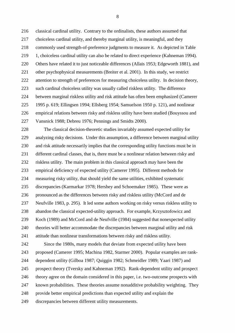
classical cardinal utility. Contrary to the ordinalists, these authors assumed that 216

choiceless cardinal utility, and thereby marginal utility, is meaningful, and they 217

commonly used strength-of-preference judgments to measure it. As depicted in Table 218

1, choiceless cardinal utility can also be related to direct experience (Kahneman 1994). 219

Others have related it to just noticeable differences (Allais 1953; Edgeworth 1881), and 220

other psychophysical measurements (Breiter et al. 2001). In this study, we restrict 221

attention to strength of preferences for measuring choiceless utility. In decision theory, 222

such cardinal choiceless utility was usually called riskless utility. The difference 223

between marginal riskless utility and risk attitude has often been emphasized (Camerer 224

1995 p. 619; Ellingsen 1994; Ellsberg 1954; Samuelson 1950 p. 121), and nonlinear 225

empirical relations between risky and riskless utility have been studied (Bouyssou and 226

Vansnick 1988; Debreu 1976; Pennings and Smidts 2000). 227

The classical decision-theoretic studies invariably assumed expected utility for 228

analyzing risky decisions. Under this assumption, a difference between marginal utility 229

and risk attitude necessarily implies that the corresponding utility functions must be in 230

different cardinal classes, that is, there must be a nonlinear relation between risky and 231

riskless utility. The main problem in this classical approach may have been the 232

empirical deficiency of expected utility (Camerer 1995). Different methods for 233

measuring risky utility, that should yield the same utilities, exhibited systematic 234

discrepancies (Karmarkar 1978; Hershey and Schoemaker 1985). These were as 235

pronounced as the differences between risky and riskless utility (McCord and de 236

Neufville 1983, p. 295). It led some authors working on risky versus riskless utility to 237

abandon the classical expected-utility approach. For example, Krzysztofowicz and 238

Koch (1989) and McCord and de Neufville (1984) suggested that nonexpected utility 239

theories will better accommodate the discrepancies between marginal utility and risk 240

attitude than nonlinear transformations between risky and riskless utility. 241

Since the 1980s, many models that deviate from expected utility have been 242

proposed (Camerer 1995; Machina 1982, Starmer 2000). Popular examples are rank-243

dependent utility (Gilboa 1987; Quiggin 1982; Schmeidler 1989; Yaari 1987) and 244

prospect theory (Tversky and Kahneman 1992). Rank-dependent utility and prospect 245

theory agree on the domain considered in this paper, i.e. two-outcome prospects with 246

known probabilities. These theories assume nonadditive probability weighting. They 247

provide better empirical predictions than expected utility and explain the 248

discrepancies between different utility measurements. 249

9

Several authors have suggested that utility measurement can be improved through 250

prospect theory (Bayoumi and Redelmeier 2000; Bleichrodt, Pinto, and Wakker 2001; 251

Krzysztofowicz and Koch 1989). Before, Fellner (1961 p. 676) suggested the same 252

basic idea. Under prospect theory, aspects of risk attitude not captured by marginal 253

utility can be explained by probability weighting, so that the main reason to distinguish 254

between risky and riskless utility disappears. The experimental findings of this paper 255

will, indeed, find no systematic difference between risky and riskless utility if the data 256

are analyzed in terms of prospect theory. 257

258

259

4. Expected Utility and Prospect Theory 260

Throughout this paper, U: — → — denotes a utility function of money that is strictly 261

increasing. We examin situations in which U is measurable or cardinal in a 262

mathematical sense, i.e. U is determined up to unit and origin. The same symbol U 263

will be used for utilities measured through strength of preferences as for utilities 264

measured through risky choices under various theories, even though a priori these 265

utilities may be different. The meaning of U will be clear from the context. The 266

different interpretations of U for strength of preference, expected utility, rank-267

dependent utility, and prospect theory (where the term value function is often used) 268

will be discussed in Section 6. 269

By (p,x; y) we denote a monetary prospect yielding outcome x with probability p 270

and outcome y otherwise. Expected utility (EU) assumes that a utility function U 271

exists such that the prospect is evaluated by pU(x) + (1−p)U(y). It is well known that 272

U is cardinal in the mathematical sense of being unique up to unit and origin.3 273

Prospect theory assumes that probabilities are weighted nonlinearly, by the 274

probability weighting function, denoted w. The prospect theory (PT) value of a 275

prospect (p,x; y) is w(p)U(x) + (1−w(p))U(y), where it is assumed that x ≥ y ≥ 0. EU 276

is the special case where w is the identity. For the prospects considered in this paper, 277

that only yield gain outcomes, original prospect theory (Kahneman & Tversky, 1979, 278

Eq. 2), rank-dependent utility (Quiggin, 1982), and their combination, cumulative 279

3 It need not be cardinal in the sense of being the neo-classical index of goodness that emerged at the end of the 19th

century (Baumol 1958 p. 655).

10

prospect theory (Tversky & Kahneman, 1992), agree. Gul's (1991) disappointment 280

theory also agrees with these theories on our domain of two-outcome prospects, and, 281

therefore, our conclusions hold under this theory as well. On the domain considered, 282

original prospect theory is not subject to the theoretical problems that have been 283

pointed out for other choices (Handa 1977; Fishburn 1978). The normalization U(0) 284

= 0, necessary in prospect theory when loss outcomes are present, is not required in 285

our domain because it does not affect preferences here. 286

Similar to the utility function, the function w is subjective and depends on the 287

individual, reflecting sensitivity towards probabilities. Many empirical investigations 288

have studied the shape of w. Figure 1 depicts the prevailing shape (Abdellaoui 2000; 289

Bleichrodt & Pinto 2000; Camerer & Ho 1994; Gonzalez & Wu 1999; Kachelmeier & 290

Shehata 1992; Karni & Safra 1990; Prelec 1998; Quiggin 1982; Tversky & Kahneman 291

1992; Yaari 1965). For counter-evidence, see Birnbaum & Navarrete (1998) and 292

Harbaugh, Krause, & Vesterlund (2002). 293

294

295

296

297

298

299

300

301

302

303

304

305

306

307

Under expected utility, all risk aversion has to be captured through concave 308

utility whereas under the descriptively more realistic prospect theory, part of the 309

observed risk aversion is due to probability weighting. This suggests that classical 310

estimations of utility are overly concave. A theoretical justification for this claim was 311

provided by Rabin (2000). Our paper will provide data that supports Rabin’s claims, 312

and will show that prospect theory can explain these data. 313

FIGURE 1. The common weighting function. p

w

1

1

0

⅓

⅓

11

314

5. An Experimental Comparison of Choice-Based and Choiceless Utilities 315

This section presents the first two measurement methods, the, choice-based, tradeoff 316

method and the, choiceless, strength-of-preference method. 317

318

Participants and Stimuli. We recruited 50 students from the department of economics 319

of the Ecole Normale Supérieure of Cachan. Each participant was paid FF 150 ($1 ≈ 320

FF 6). No performance-based payments could be used for reasons discussed in 321

Section 7. Each participant was interviewed individually by means of a computer 322

program, in the presence of the experimenter. The participants were familiar with 323

probabilities and expectations but had not received a training in decision theory before 324

the experiment. Prior to the experimental questions, the participants were 325

familiarized with the stimuli through some practice questions. Three participants 326

were discarded because they gave erratic answers and apparently did not understand 327

the instructions; N = 47 participants remained. 328

Our choice-based method concerns risky choices. Only degenerate or two-329

outcome prospects were used. They were displayed as pie charts on a computer 330

screen, where different colors were used to designate different areas; see Appendix A. 331

The units of payment in the prospects were French Francs. At the beginning of the 332

experiment, a random device repeatedly picked random points from the pie charts so 333

as to familiarize the participants with the representation of probabilities used in this 334

experiment. 335

The measurements of this paper are based on indifferences. It is well known that 336

observations of indifferences are prone to many biases, in particular if derived from 337

direct matching. Indifferences derived from choices seem to be less prone to biases 338

(Bostic, Herrnstein, & Luce 1990; Tversky & Kahneman 1992 p. 306). We 339

developed software for carefully observing indifferences while avoiding biases. 340

Appendix A gives details. We assessed three to six points for fitting the utility 341

functions; using such numbers of points was recommended by von Winterfeldt & 342

Edwards (1986, p. 254). 343

We used a within-subject design, with all measurements carried out for all 344

individuals. All statistical analyses are based on within-subject differences. The 345

tradeoff method was always carried out before the other methods because its answers 346

12

served as inputs in further elicitations, so as to simplify the comparisons. The order 347

of the other methods was counterbalanced so as to minimize systematic memory 348

effects, which is especially important for the strength of preference measurements. 349

350

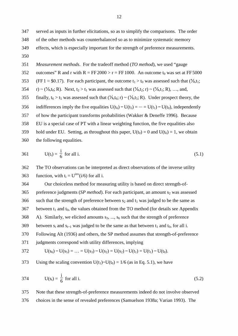
Measurement methods. For the tradeoff method (TO method), we used “gauge 351

outcomes” R and r with R = FF 2000 > r = FF 1000. An outcome t0 was set at FF 5000 352

(FF 1 ≈ $0.17). For each participant, the outcome t1 > t0 was assessed such that (⅓,t1; 353

r) ~ (⅓,t0; R). Next, t2 > t1 was assessed such that (⅓,t2; r) ~ (⅓,t1; R), …, and, 354

finally, t6 > t5 was assessed such that (⅓,t6; r) ~ (⅓,t5; R). Under prospect theory, the 355

indifferences imply the five equalities U(t6) − U(t5) = ... = U(t1) − U(t0), independently 356

of how the participant transforms probabilities (Wakker & Deneffe 1996). Because 357

EU is a special case of PT with a linear weighting function, the five equalities also 358

hold under EU. Setting, as throughout this paper, U(t0) = 0 and U(t6) = 1, we obtain 359

the following equalities. 360

U(ti) = i6 for all i. (5.1) 361

The TO observations can be interpreted as direct observations of the inverse utility 362

function, with ti = Uinv(i/6) for all i. 363

Our choiceless method for measuring utility is based on direct strength-of-364

preference judgments (SP method). For each participant, an amount s2 was assessed 365

such that the strength of preference between s2 and t1 was judged to be the same as 366

between t1 and t0, the values obtained from the TO method (for details see Appendix 367

A). Similarly, we elicited amounts s3, ..., s6 such that the strength of preference 368

between si and si−1 was judged to be the same as that between t1 and t0, for all i. 369

Following Alt (1936) and others, the SP method assumes that strength-of-preference 370

judgments correspond with utility differences, implying 371

U(s6) − U(s5) = … = U(s3) − U(s2) = U(s2) − U(t1) = U(t1) − U(t0). 372

Using the scaling convention U(t1)−U(t0) = 1/6 (as in Eq. 5.1), we have 373

U(si) = i6 for all i. (5.2) 374

Note that these strength-of-preference measurements indeed do not involve observed 375

choices in the sense of revealed preferences (Samuelson 1938a; Varian 1993). The 376

13

various attempts to relate strength-of-preference judgments to choice making in a 377

theoretical model after all, through side payments such as hours of labor, repeated or 378

probabilistic choices, etc., are all based on separability assumptions that beg the 379

question of cardinal utility. Strengths of preferences have, therefore, not been part of 380

the commonly accepted empirical domain under the ordinal view of utility. 381

382

Analysis. In each test in this paper, the null hypothesis H0 assumes identical utility 383

functions for the various methods. For testing group averages, we considered paired 384

t-tests and Wilcoxon signed rank tests, all two-tailed, which always gave the same 385

results. Conclusions based on accepted null hypotheses are most convincing under 386

the most powerful tests, i.e. the t-tests. Hence, we usually report those. To reckon 387

with individual differences, our main conclusions, presented in later sections, will be 388

based on analysis of variance with repeated measures whenever possible. These 389

analyses always give the same conclusions as paired t-tests. 390

391

392

393

394

395

396

397

398

399

400

401

402

403

404

405

406

407

408

409

410 FIGURE 2. A choice-based and a choiceless utility function (for mean values).

t0= FF 5,000 0,00

0,17

0,33

0,50

0,67

0,83

1,00

1,16

FF

U

t6= FF 26,068

choice- based (TO)

choice- less (SP)

14

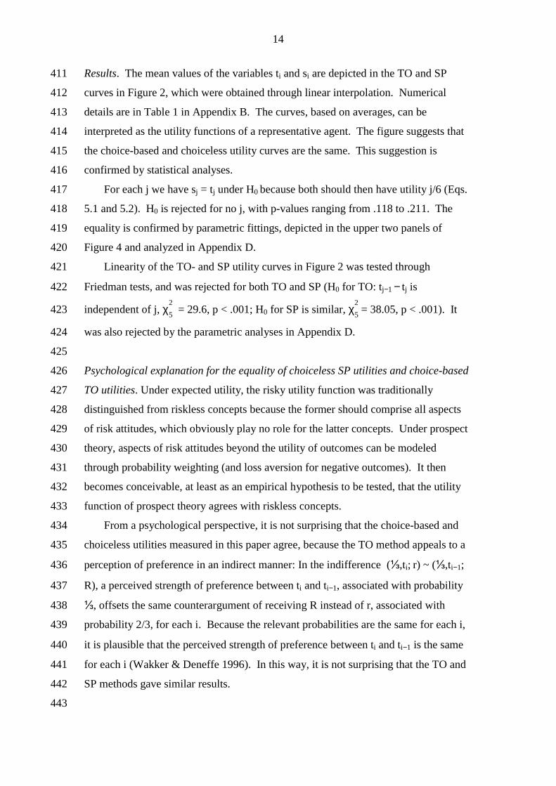
Results. The mean values of the variables ti and si are depicted in the TO and SP 411

curves in Figure 2, which were obtained through linear interpolation. Numerical 412

details are in Table 1 in Appendix B. The curves, based on averages, can be 413

interpreted as the utility functions of a representative agent. The figure suggests that 414

the choice-based and choiceless utility curves are the same. This suggestion is 415

confirmed by statistical analyses. 416

For each j we have sj = tj under H0 because both should then have utility j/6 (Eqs. 417

5.1 and 5.2). H0 is rejected for no j, with p-values ranging from .118 to .211. The 418

equality is confirmed by parametric fittings, depicted in the upper two panels of 419

Figure 4 and analyzed in Appendix D. 420

Linearity of the TO- and SP utility curves in Figure 2 was tested through 421

Friedman tests, and was rejected for both TO and SP (H0 for TO: tj−1 − tj is 422

independent of j, χ5

2 = 29.6, p < .001; H0 for SP is similar, χ

5

2 = 38.05, p < .001). It 423

was also rejected by the parametric analyses in Appendix D. 424

425

Psychological explanation for the equality of choiceless SP utilities and choice-based 426

TO utilities. Under expected utility, the risky utility function was traditionally 427

distinguished from riskless concepts because the former should comprise all aspects 428

of risk attitudes, which obviously play no role for the latter concepts. Under prospect 429

theory, aspects of risk attitudes beyond the utility of outcomes can be modeled 430

through probability weighting (and loss aversion for negative outcomes). It then 431

becomes conceivable, at least as an empirical hypothesis to be tested, that the utility 432

function of prospect theory agrees with riskless concepts. 433

From a psychological perspective, it is not surprising that the choice-based and 434

choiceless utilities measured in this paper agree, because the TO method appeals to a 435

perception of preference in an indirect manner: In the indifference (⅓,ti; r) ~ (⅓,ti−1; 436

R), a perceived strength of preference between ti and ti−1, associated with probability 437

⅓, offsets the same counterargument of receiving R instead of r, associated with 438

probability 2/3, for each i. Because the relevant probabilities are the same for each i, 439

it is plausible that the perceived strength of preference between ti and ti−1 is the same 440

for each i (Wakker & Deneffe 1996). In this way, it is not surprising that the TO and 441

SP methods gave similar results. 442

443

15

6. Verifying the Validity of Measurements 444

A pessimistic interpretation of the equality found in the preceding section can be 445

devised, in agreement with the constructive view of preference (Gregory, 446

Lichtenstein, & Slovic 1993; Loomes, Starmer, & Sugden 2003): The participants 447

may simply have used similar heuristics in both methods used, and their TO answers 448

may not reflect genuine preference. To investigate this possibility, we used a third, 449

traditional, method for measuring utility, a certainty-equivalent method. For the first 450

13 participants, only TO and SP measurements were conducted. Then it was realized 451

that further questions were feasible. Therefore, for the remaining 34 participants not 452

only TO and SP measurements, but also two certainty equivalent measurements were 453

conducted. 454

455

456

457

458

459

460

461

462

463

464

465

466

467

468

469

470

471

472

473

474

Certainty-equivalent methods compare sure amounts of money to two-outcome 475

prospects and have been used in many studies (von Winterfeldt & Edwards 1986). 476

FIGURE 3. All utility functions (for mean values).

t0= FF 5,000 0,00

0,17

0,33

0,50

0,67

0,83

1,00

1,16

FF

U

t6= FF 26,068

CE1/3

CE 2/3 (EU)

CE 2/3 (PT) SP

TO

16

They have a format different than TO and SP methods. Therefore, if heuristics are 477

used, it is plausible that they will be different for certainty equivalents than for the TO 478

and SP methods, and that they will not generate the same utilities. The third method 479

considered prospects that assign probability 1/3 to the best outcome. The reason for 480

this particular choice of probability will be explained at the end of this section. The 481

third method is called the CE1/3 method. Amounts c2, c1, and c3 were elicited such 482

that c2 ~ (⅓,t6; t0), c1 ~ (⅓,c2; t0), and c3 ~ (⅓,t6; c2). 483

We first analyze this method in the classical manner, i.e., assuming EU. We will 484

see later that the following equalities and analysis remain valid under prospect theory. 485

With U(t0) = 0 and U(t6) = 1, we get: 486

U(c2) = 13 , U(c1) =

19 , and U(c3) =

59 . (6.1) 487

All nonparametric utility curves measured in our experiment, based on group averages 488

and linear interpolation, are assembled in Figure 3. Figure 4 gives the average result 489

of parametric fittings, explained in Appendix C. The figures suggest that the average 490

utility function resulting from the CE1/3 observations agrees well with the TO and SP 491

utility functions. Analysis of variance with repeated measures for the parametric 492

fittings confirms the equality of the TO, SP, and CE1/3 measurements while taking 493

into account differences at the individual level, with F(2, 66) = 0.54, p = 0.58. The 494

same conclusion follows from other statistical analyses reported in Appendices B and 495

D. 496

At this point, two concerns can be raised. First, it may be argued that the 497

assumption of EU used in the preceding analysis is not descriptively valid. Second, it 498

may be conjectured that our design does not have the statistical power to detect 499

differences (apart from nonlinearity of the utility curves). To investigate these 500

concerns, we used a fourth method for measuring utility, another certainty-equivalent 501

method. This method considered prospects that assign probability 2/3 to the best 502

outcome and is, therefore, called the CE2/3 method. The same 34 individuals 503

participated as in the CE1/3 method. Amounts d2, d1, and d3 were elicited such that d2 504

~ (⅔,t6; t0), d1 ~ (⅔,d2; t0), and d3 ~ (⅔,t6; d2). We first analyze this method assuming 505

EU. With U(t0) = 0 and U(t6) = 1, the following equalities are implied. 506

U(d1) = 49, U(d2) =

23, and U(d3) =

89 . (6.2) 507

17

The average utility function resulting from the CE2/3 observations under EU is 508

depicted as the CE2/3(EU) curve in Figure 3 for linear interpolation, and in the middle 509

right panel in Figure 4. The function strongly deviates from the other curves. 510

Whereas analysis of variance with repeated measures for the parametric fittings 511

concluded that the three measurements (TO, SP, CE1/3) are the same, addition of 512

CE2/3(EU) leads to the conclusion that the four measurements (TO, SP, CE1/3, 513

CE2/3(EU)) are not the same, F(3,99) = 6.39, p = 0.001. That CE2/3(EU) is different 514

from the other measurements, is confirmed by other statistical analyses, such as 515

pairwise comparisons, presented in Appendices B and D. This finding falsifies EU 516

and agrees with the EU violations documented in the literature. 517

We reanalyze the results of the certainty-equivalent methods by means of 518

prospect theory, and correct the utility measurements for probability weighting. Such 519

corrections were suggested before by Fellner (1961, p. 676), Wakker & Stiggelbout 520

(1995), Stalmeier & Bezembinder (1999), and Bleichrodt, Pinto, & Wakker (2001). 521

We assume the probability weighting function of Figure 1 for all individuals. This 522

assumption obviously is an approximation because in reality the probability weighting 523

function will depend on the individual. The descriptive performance of prospect 524

theory could be improved if information about individual probability weighting were 525

available. In the absence of such information, we expect that, on average, PT with the 526

probability weighting function of Figure 1 will yield better results than EU, which 527

also assumes that the weighting function is the same for all individuals but, 528

furthermore, assumes that it is linear. Let us repeat that the analysis of the TO method 529

remains valid under PT, irrespective of the individual probability weighting functions. 530

Therefore, contrary to the CE methods, it is not affected by individual variations in 531

probability weighting. 532

533

534

18

534

535

536

537

538

539

540

541

542

543

544

545

546

547

548

549

550

551

552

553

554

555

556

557

558

559

560

561

562

563

564

565

566

t0 = FF 5,000

t6 = FF 26,810

0

1

U

t0 = FF 5,000

t6 = FF 26,810

0

1

U

CE2/3 (PT)

FIGURE 4. Mean results for the expo-power family.

CE1/3 (EU & PT)

t0 = FF 5,000

t6 = FF 26,810

0

1

U TO

t0 = FF 5,000

t6 = FF 26,810

0

1

U

CE2/3 (EU)

s0 = FF 5,000

s6 = FF 30,161

0

1

U

SP

19

566

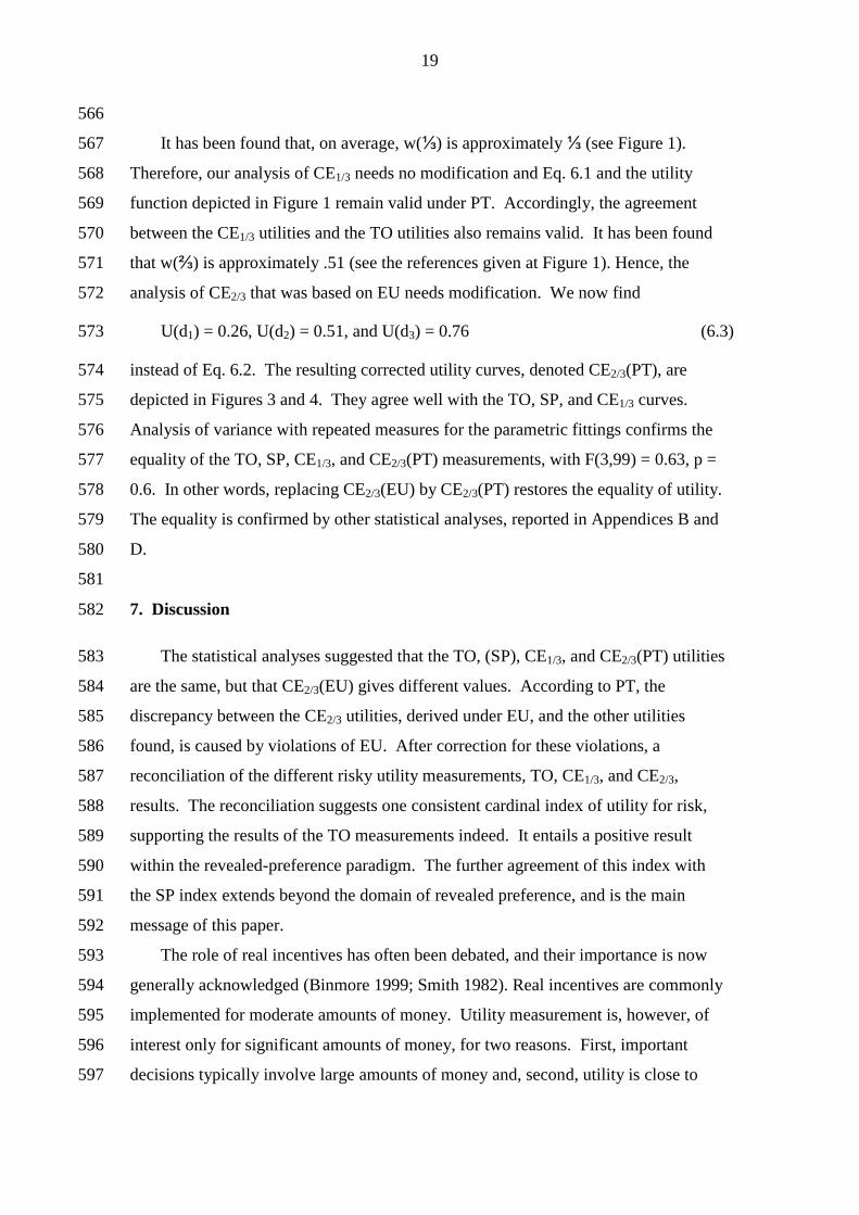
It has been found that, on average, w(⅓) is approximately ⅓ (see Figure 1). 567

Therefore, our analysis of CE1/3 needs no modification and Eq. 6.1 and the utility 568

function depicted in Figure 1 remain valid under PT. Accordingly, the agreement 569

between the CE1/3 utilities and the TO utilities also remains valid. It has been found 570

that w(⅔) is approximately .51 (see the references given at Figure 1). Hence, the 571

analysis of CE2/3 that was based on EU needs modification. We now find 572

U(d1) = 0.26, U(d2) = 0.51, and U(d3) = 0.76 (6.3) 573

instead of Eq. 6.2. The resulting corrected utility curves, denoted CE2/3(PT), are 574

depicted in Figures 3 and 4. They agree well with the TO, SP, and CE1/3 curves. 575

Analysis of variance with repeated measures for the parametric fittings confirms the 576

equality of the TO, SP, CE1/3, and CE2/3(PT) measurements, with F(3,99) = 0.63, p = 577

0.6. In other words, replacing CE2/3(EU) by CE2/3(PT) restores the equality of utility. 578

The equality is confirmed by other statistical analyses, reported in Appendices B and 579

D. 580

581

7. Discussion 582

The statistical analyses suggested that the TO, (SP), CE1/3, and CE2/3(PT) utilities 583

are the same, but that CE2/3(EU) gives different values. According to PT, the 584

discrepancy between the CE2/3 utilities, derived under EU, and the other utilities 585

found, is caused by violations of EU. After correction for these violations, a 586

reconciliation of the different risky utility measurements, TO, CE1/3, and CE2/3, 587

results. The reconciliation suggests one consistent cardinal index of utility for risk, 588

supporting the results of the TO measurements indeed. It entails a positive result 589

within the revealed-preference paradigm. The further agreement of this index with 590

the SP index extends beyond the domain of revealed preference, and is the main 591

message of this paper. 592

The role of real incentives has often been debated, and their importance is now 593

generally acknowledged (Binmore 1999; Smith 1982). Real incentives are commonly 594

implemented for moderate amounts of money. Utility measurement is, however, of 595

interest only for significant amounts of money, for two reasons. First, important 596

decisions typically involve large amounts of money and, second, utility is close to 597

20

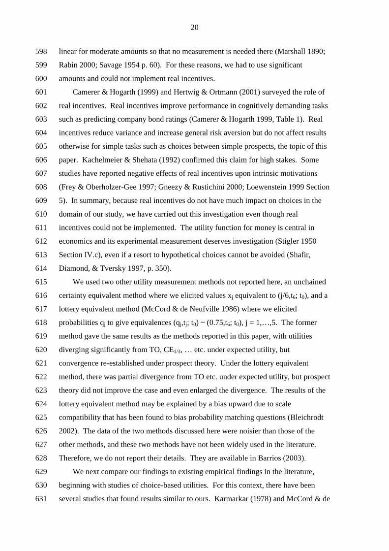
linear for moderate amounts so that no measurement is needed there (Marshall 1890; 598

Rabin 2000; Savage 1954 p. 60). For these reasons, we had to use significant 599

amounts and could not implement real incentives. 600

Camerer & Hogarth (1999) and Hertwig & Ortmann (2001) surveyed the role of 601

real incentives. Real incentives improve performance in cognitively demanding tasks 602

such as predicting company bond ratings (Camerer & Hogarth 1999, Table 1). Real 603

incentives reduce variance and increase general risk aversion but do not affect results 604

otherwise for simple tasks such as choices between simple prospects, the topic of this 605

paper. Kachelmeier & Shehata (1992) confirmed this claim for high stakes. Some 606

studies have reported negative effects of real incentives upon intrinsic motivations 607

(Frey & Oberholzer-Gee 1997; Gneezy & Rustichini 2000; Loewenstein 1999 Section 608

5). In summary, because real incentives do not have much impact on choices in the 609

domain of our study, we have carried out this investigation even though real 610

incentives could not be implemented. The utility function for money is central in 611

economics and its experimental measurement deserves investigation (Stigler 1950 612

Section IV.c), even if a resort to hypothetical choices cannot be avoided (Shafir, 613

Diamond, & Tversky 1997, p. 350). 614

We used two other utility measurement methods not reported here, an unchained 615

certainty equivalent method where we elicited values xj equivalent to (j/6,t6; t0), and a 616

lottery equivalent method (McCord & de Neufville 1986) where we elicited 617

probabilities qj to give equivalences (qj,tj; t0) ~ (0.75,t6; t0), j = 1,…,5. The former 618

method gave the same results as the methods reported in this paper, with utilities 619

diverging significantly from TO, CE1/3, … etc. under expected utility, but 620

convergence re-established under prospect theory. Under the lottery equivalent 621

method, there was partial divergence from TO etc. under expected utility, but prospect 622

theory did not improve the case and even enlarged the divergence. The results of the 623

lottery equivalent method may be explained by a bias upward due to scale 624

compatibility that has been found to bias probability matching questions (Bleichrodt 625

2002). The data of the two methods discussed here were noisier than those of the 626

other methods, and these two methods have not been widely used in the literature. 627

Therefore, we do not report their details. They are available in Barrios (2003). 628

We next compare our findings to existing empirical findings in the literature, 629

beginning with studies of choice-based utilities. For this context, there have been 630

several studies that found results similar to ours. Karmarkar (1978) and McCord & de 631

21

Neufville (1986) found that utilities, measured through certainty equivalents with 632

different probabilities, are inconsistent when analyzed by means of EU. Abdellaoui 633

(2000) found that the utilities measured by the TO method are not affected by 634

probability weighting. Bleichrodt, Pinto, & Wakker (2001) found that corrections by 635

means of the probability weighting function of Figure 1 reconcile discrepancies 636

between choice-based utilities. Tversky & Fox (1995 p. 276) pointed out the 637

appealing feature of the ⅓ probability that it does not lead to systematic probability 638

transformations in CE questions. Finally, Rabin (2000) argued on theoretical grounds 639

that utility is more linear than commonly thought, and that most of the commonly 640

observed risk aversion is due to factors other than utility curvature. 641

Rabin's argument is based on a paradox entailing that, if risk attitude is based 642

solely on utility curvature as in expected utility, then a moderate and realistic degree 643

of risk aversion for moderate stakes necessarily implies an extreme and unrealistic 644

degree of risk aversion for high stakes. We used prospect theory, where risk attitude 645

consists of other factors besides utility curvature, to estimate the utility function. Our 646

empirical findings of moderate utility curvature confirm Rabin's predictions. Our 647

contribution to Rabin’s paradox is to demonstrate that not only does it refute expected 648

utility, but also it can be accommodated by prospect theory. 649

For the economic literature, the novelty of our study lies in the comparison of 650

choice-based utilities, derived from prospect theory, with choiceless utilities derived 651

from strength-of-preference judgments. The direct agreement between these 652

measurements (alluded to by Camerer 1995, p. 625) is remarkable. Our 653

measurements satisfy Birnbaum & Sutton's (1992) principle of scale convergence, 654

according to which different ways to measure utility should give the same result. It 655

would, indeed, be desirable if one concept of utility could emerge that is relevant for 656

many contexts, such as decision under risk, welfare evaluations, intertemporal 657

discounted utility, case-based reasonings (Gilboa & Schmeidler 1995), etc. (cf. 658

Broome's 1991 index of goodness, or Robson 2001). 659

In applied domains, e.g. in health economics, it is common practice to use 660

utilities measured in one context for applications in other contexts (Gold et al. 1996; 661

Torrance, Boyle, & Horwood 1982). For example, risky utilities measured through 662

the "standard gamble method" have been used in policy decisions about interpersonal 663

tradeoffs (treating elderly versus young people) or intertemporal decisions (current 664

prevention measures against future health impairments). Also choiceless utilities, 665

22

measured through direct scaling questions or otherwise, have been used for decision 666

making. The pragmatic justification is that no better data are available, and decisions 667

have to be taken as good as possible with whatever is available. Empirical relations 668

between various utilities have been studied extensively. See Frey & Stutzer (2000 p. 669

920), Pennings & Smidts (2000), Revicki & Kaplan (1993), Robinson, Loomes, & 670

Jones-Lee (2001). Our improved procedures based on prospect theory provide a new 671

way of studying such relationships. 672

We only compared risky choice-based utilities to riskless choiceless utilities 673

derived from strengths of preferences, and we did not consider utilities derived from 674

other tradeoffs such as interpersonal or intertemporal. We hope that future empirical 675

studies will consider such other tradeoffs, and that Birnbaum and Broome's scale 676

convergence can be established with one unified concept of utility relevant to many 677

domains in social sciences. Then the use of choiceless data in applications, such as 678

health economics, can become more acceptable to mainstream economists and 679

ordinalists, not only for pragmatic reasons (Manski 2004), but also conceptually. 680

681

8. Conclusion 682

In the classical economic debate between cardinalists and ordinalists, the latter 683

assumed that direct judgments, having no preference basis, are not meaningful. In the 684

light of today’s advances in experimental methods in economics, the question whether 685

relations exist between direct judgments and preferences can be investigated 686

empirically. The first investigations of such relations were conducted in decision 687

theory. These investigations assumed expected utility theory, so that their results 688

were distorted by the descriptive deficiencies of this theory. Prospect theory provided 689

descriptive improvements. Using this theory, our experiment suggests a simple 690

relation between direct strength-of-preference judgments and risky-decision utilities. 691

If an empirical relationship between direct judgments and preferences can be 692

firmly established, then direct judgments will provide useful data for economic 693

analyses in contexts where preferences are hard to measure because of choice 694

anomalies (Kahneman 1994). Conversely, such links provide a consistency basis for 695

direct judgments. The result will be that direct judgments reinforce the revealed 696

preference approach and vice versa. We, therefore, hope for further empirical 697

investigations of the relations between direct judgments and revealed preferences. 698

23

699

Appendix A. A Two-Step Procedure for Eliciting Indifferences 700

This appendix describes the new two-step procedure that was developed so as to obtain 701

reliable indifferences. We first consider the measurement of t1 for the TO method. That 702

is, a value x (= t1) was to be found to yield an indifference A = (1/3,5000; 2000) ~ 703

(1/3,x; 1000) = B. Figure 5 displays these prospects (called propositions there) for x = 704

11000. The first step of our procedure established an interval containing t1. It started 705

with x = 5000, which clearly is a lowerbound for t1 because the right prospect B then is 706

dominated by the left prospect A. By means of a scrollbar, the experimenter next 707

increased x to 25000, and here all participants preferred the right prospect B, so that 708

25000 is an upper bound for t1 for all participants. These questions, yielding a 709

preliminary interval [5000, 25000] containing t1, served only to familiarize the subjects 710

with the choices. The interval containing t1 that we searched for was to be a narrower 711

subinterval of [5000, 25000], and was obtained as follows. 712

The scrollbar was again placed at its initial value x = 5000, where B is dominated 713

by A. The experimenter increased x until the participant was no longer sure that she 714

prefers A. Next a smaller outcome x was found for which the participant was still sure 715

to prefer A to B, say x = a > 5000. Similarly, an outcome x of B was found for which 716

the participant was sure to prefer B to A, say x = b < 25000. Obviously, b > a; if not, 717

the participant did not understand the procedure and it was repeated. Thus, an interval 718

[a, b] was obtained that contained the indifference value t1. We wanted this interval to 719

be of the same length for all participants. Hence, we asked participants to be more 720

precise if their interval [a, b] was too long. Commonly it was shorter, in which case the 721

computer automatically enlarged it. In this manner, an interval of a fixed length was 722

obtained for the second step. Figure 5 displays the final result of Step 1 for a participant 723

with [a, b] = [7000, 11000] as the interval of fixed length containing t1. 724

725

24

725

726

727

728

729

730

731

732

733

734

735

736

737

738

739

740

741

742

743

744

745

746

747

748

749

750

751

752

753

754

755

Choose the preferred proposition (A or B) and click on the corresponding button. Then please confirm your choice.

*** We are only interested in your preferences. **** There are no right or wrong answers.

FF 5000

ff5000

FF 2000

ff5000

33%

ff5000 67%

ff5000

Proposition A

FF 9000

ff5000

FF 1000

ff5000

33%

ff5000 67%

ff5000

Proposition B

You have chosen Proposition: B Confirm

FIGURE 6. Presentation of the prospects in the second step.

FF 5000

ff5000

FF 2000

ff5000

33%

ff5000 67%

ff5000

Proposition A

FF 11000

ff5000

FF 1000

ff5000

33%

ff5000 67%

ff5000

Proposition B

Do you still prefer proposition A?

FIGURE 5. A screen used in the first step.

Do you still prefer proposition B? Change

Confirm 7000 yes 11000 yes

25

In Step 2 of our procedure to elicit t1, a choice-based bisection procedure was 756

used to find the indifference value x = t1 ∈ [α,β]; see Figure 6. The midpoint (α+β)/2 757

of the interval of Step 1 was substituted for x, and the participant was asked to choose 758

between the prospects—indifference was not permitted. The midpoint was 759

subsequently combined with the left or right endpoint of the preceding interval, 760

depending on the preference expressed. In this manner, a new interval resulted that 761

contained t1 and that was half as large as the preceding interval. After five similar 762

iterations, the interval was sufficiently narrow and its midpoint was taken as t1. To 763

test for consistency, we repeated the choice of the third iteration; it was virtually 764

always (≥ 92% for each measurement) consistent in our experiment. 765

766

767

768

769

770

771

772

773

774

775

776

777

778

779

780

781

782

783

784

FIGURE 7. Presentation of strength of preference questions.

Initial Situation Final Situation

Change A

Change B

FF 5000 FF 6800

FF 6800 FF 14800

Which is the most important change (A or B) for you? Please confirm your choice.

*** We are only interested in your preferences. **** There are no right or wrong answers.

You have chosen Change: B Confirm

26

784

785

786

787

788

789

790

791

792

793

794

795

796

797

798

799

We adopted the above elaborate method of eliciting indifference values so as to 800

obtain high-quality data, avoiding many biases that have been known to arise from 801

direct matching questions (Bostic, Herrnstein, & Luce 1990). The indifference values 802

t2,…,t6 were elicited similarly. For the CE measurements we used the same way to 803

elicit indifferences as for the TO measurements, now with one option being riskless. 804

For the strength-of-preference measurements, a similar two-stage procedure was used 805

but the stimuli were different because no prospects were involved. Figures 7 and 8 806

show the screens presented to the participants in the two stages. 807

808

Appendix B. Statistical Analysis of Raw Data 809

Table 1 gives descriptive statistics of our measurements. Paired t-tests of the 810

equality of TO and SP measurements were described in the main text. We next 811

consider paired t-test comparisons of the other two measurements with TO. 812

813

FIGURE 8. Presentation of strength of preference questions.

Change

10800 yes 14800 yes

Initial Situation Final Situation

Change A

Change B

FF 5000 FF 6800

FF 6800 FF 14800

Do you still consider change A to be more important?

Do you still consider change B to be more important?

27

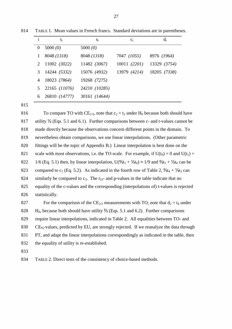
TABLE 1. Mean values in French francs. Standard deviations are in parentheses. 814

i ti si ci di

0 5000 (0) 5000 (0)

1 8048 (1318) 8048 (1318) 7047 (1055) 8976 (1964)

2 11002 (3022) 11482 (3067) 10011 (2201) 13329 (3754)

3 14244 (5332) 15076 (4932) 13979 (4214) 18205 (7338)

4 18023 (7864) 19268 (7275)

5 22165 (11076) 24210 (10285)

6 26810 (14777) 30161 (14644)

815

To compare TO with CE1/3, note that c2 = t2 under H0 because both should have 816

utility ⅓ (Eqs. 5.1 and 6.1). Further comparisons between c- and t-values cannot be 817

made directly because the observations concern different points in the domain. To 818

nevertheless obtain comparisons, we use linear interpolations. (Other parametric 819

fittings will be the topic of Appendix B.) Linear interpolation is best done on the 820

scale with most observations, i.e. the TO scale. For example, if U(t0) = 0 and U(t1) = 821

1/6 (Eq. 5.1) then, by linear interpolation, U(⅔t1 + ⅓t0) ≈ 1/9 and ⅔t1 + ⅓t0 can be 822

compared to c1 (Eq. 5.2). As indicated in the fourth row of Table 2, ⅔t4 + ⅓t3 can 823

similarly be compared to c3. The t33- and p-values in the table indicate that no 824

equality of the c-values and the corresponding (interpolations of) t-values is rejected 825

statistically. 826

For the comparison of the CE2/3 measurements with TO, note that d2 = t4 under 827

H0, because both should have utility ⅔ (Eqs. 5.1 and 6.2). Further comparisons 828

require linear interpolations, indicated in Table 2. All equalities between TO- and 829

CE⅔-values, predicted by EU, are strongly rejected. If we reanalyze the data through 830

PT, and adapt the linear interpolations correspondingly as indicated in the table, then 831

the equality of utility is re-established. 832

833

TABLE 2. Direct tests of the consistency of choice-based methods. 834

28

theory CEs Utility TOs* t33 p-value

EU & PT c1 1/9 ⅔t1+⅓t0 0.09 .928

EU& PT c2 1/3 t2 −1.49 .146

EU& PT c3 5/9 ⅓t4+⅔t3 −1.52 .138 EU d1 4/9 ⅔t3+⅓t2 −5.41 .000

EU d2 2/3 t4 −4.30 .000

EU d3 8/9 ⅓t6+⅔t5 −3.96 .000 PT d1 0.26 .58 t2 + .42 t1 −1.45 .158

PT d2 0.51 .08 t4 + .92 t3 −1.19 .244

PT d3 0.76 .58 t5 + .42 t4 −1.78 .084 *: interpolated ti's 835

836

All tests in this appendix confirm the conclusions based on analysis of variance 837

with repeated measures, reported in the main text. Nevertheless, a number of 838

objections can be raised against the analyses of this appendix. For the scale that is 839

interpolated, a bias downward is generated because utility is usually concave and not 840

linear. For scales with few observations such as the CE scales, the bias can be big 841

and, therefore, a direct comparison of CE1/3 and CE2/3 is not well possible. The latter 842

problem is aggrevated because the different CE measurements focus on different parts 843

of the domain. 844

The pairwise comparisons of the different points in Table 2 are not independent 845

because the measurements are chained. Biases in measurements may propagate. This 846

may explain why all five sj values in Table 1 exceed the corresponding tj values, 847

although the difference is never significant. The differences can be explained by an 848

overweighting of t0 and t1, due to their role as anchor outcomes in the SP 849

measurements. While distorting the sj's upwards, this bias hardly distorts the elicited 850

utility curvature. For the latter, not the values of sj or tj per se, but their equal 851

spacedness in utility units, is essential. This equal spacedness is affected only for the 852

interval [U(t0),U(t1)] under the SP method, which then is somewhat underestimated. 853

For these reasons, it is preferable to investigate the curvature of utility, as opposed to 854

the directly observed inverse utility values (this is what our observations ti, si, ci, di, in 855

fact are). We investigate the curvature of utility through parametric fittings in the 856

following appendices. 857

29

858

Appendix C. Fitting Parametric Utility Families 859

We fitted a number of parametric families to our data, and used the resulting 860

parameters in the statistical analyses. All families hereafter were normalized so as to 861

be on a same scale, and in this manner their numerical fits were compared. Because 862

normalizations do not affect the empirical meaning of cardinal utility, we give non-863

normalized formulas hereafter as their notation is simpler. First, we considered the 864

two families that have been used most frequently in the literature. Parametric fittings 865

directly concern the curvature of utility, and smoothen out irregularities in the data. A 866

drawback is that the results may depend on the particular parametric families chosen. 867

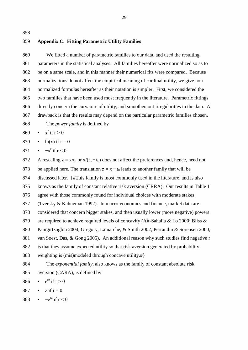
The power family is defined by 868

• xr if r > 0 869

• ln(x) if r = 0 870

• −xr if r < 0. 871

A rescaling z = x/t6 or x/(t6 − t0) does not affect the preferences and, hence, need not 872

be applied here. The translation z = x − t0 leads to another family that will be 873

discussed later. {#This family is most commonly used in the literature, and is also 874

knows as the family of constant relative risk aversion (CRRA). Our results in Table 1 875

agree with those commonly found for individual choices with moderate stakes 876

(Tversky & Kahneman 1992). In macro-economics and finance, market data are 877

considered that concern bigger stakes, and then usually lower (more negative) powers 878

are required to achieve required levels of concavity (Aït-Sahalia & Lo 2000; Bliss & 879

Panigirtzoglou 2004; Gregory, Lamarche, & Smith 2002; Perraudin & Sorensen 2000; 880

van Soest, Das, & Gong 2005). An additional reason why such studies find negative r 881

is that they assume expected utility so that risk aversion generated by probability 882

weighting is (mis)modeled through concave utility.#} 883

The exponential family, also knows as the family of constant absolute risk 884

aversion (CARA), is defined by 885

• erz if r > 0 886

• z if r = 0 887

• −erz if r < 0 888

30

where the domain [t0,t6] is mapped into the unit interval through the transformation z 889

= (x − t0)/(t6 − t0). 890

Several authors have suggested that utility is logarithmic (Bernoulli 1738; Savage 891

1954 p. 94) but this family did not fit our data well. It allows for concave utility only, 892

whereas several participants exhibited convexities. Let us recall here that utility 893

functions, when corrected for probability weighting, are less concave than traditional 894

measurements have suggested. We also considered the translated power family where 895

x is replaced by x − t0. This family supported the empirical hypotheses of this paper 896

equally well. We do not report its results because this family seems to be of limited 897

empirical interest: Its derivatives at t0 are extreme and the domain is not easily 898

extended below t0. 899

We introduce a new, third, parametric family, which we call the expo-power 900

family, and which is defined by 901

−exp(−zr

r ) for r≠0;4 902

−1z for r = 0. 903

We rescaled z = xt6

. Figure 9 depicts some examples. 904

The expo-power family is a variation of a two-parameter family introduced by 905

Saha (1993). The rescaling z = xt6

maps our domain [t0,t6] to [t0/t6,1] ⊂ [0,1]. On 906

[0,1], the family exhibits some desirable features. 907

• r has a clear interpretation, being an anti-index of concavity (the smaller r the 908

more concave the function is). 909

• The family allows for both concave (r ≤ 1) and convex (r ≥ 2) functions. 910

• There exists a subclass of this family (0 ≤ r ≤ 1) that combines a number of 911

desirable features. 912

(i) The functions are concave; 913

(ii) The measure of absolute risk aversion, the Arrow-Pratt measure −u''(x)/u'(x) 914

= (1−r)/x + xr−1, is decreasing in x. 915

4 For r close to zero, the strategically equivalent function −exp(−zr

r +1/r) is more tractable for numerical purposes.

31

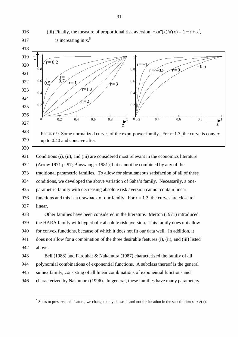
(iii) Finally, the measure of proportional risk aversion, −xu''(x)/u'(x) = 1 − r + xr, 916

is increasing in x.5 917

918

919

920

921

922

923

924

925

926

927

928

929

930

Conditions (i), (ii), and (iii) are considered most relevant in the economics literature 931

(Arrow 1971 p. 97; Binswanger 1981), but cannot be combined by any of the 932

traditional parametric families. To allow for simultaneous satisfaction of all of these 933

conditions, we developed the above variation of Saha’s family. Necessarily, a one-934

parametric family with decreasing absolute risk aversion cannot contain linear 935

functions and this is a drawback of our family. For r = 1.3, the curves are close to 936

linear. 937

Other families have been considered in the literature. Merton (1971) introduced 938

the HARA family with hyperbolic absolute risk aversion. This family does not allow 939

for convex functions, because of which it does not fit our data well. In addition, it 940

does not allow for a combination of the three desirable features (i), (ii), and (iii) listed 941

above. 942

Bell (1988) and Farquhar & Nakamura (1987) characterized the family of all 943

polynomial combinations of exponential functions. A subclass thereof is the general 944

sumex family, consisting of all linear combinations of exponential functions and 945

characterized by Nakamura (1996). In general, these families have many parameters 946

5 So as to preserve this feature, we changed only the scale and not the location in the substitution x # z(x).

0

0.2

0.4

0.6

0.8

1

0.2 0.4 0.6 0.8 1 0

0.2

0.4

0.6

0.8

1

0.2 0.4 0.6 0.8 1

r = −1 r = −0.5

r = 0.2

r = 0.5

r = 0.7 r = 1

r=1.3

r = 2

r = 3

r = 0.5 r = 0

FIGURE 9. Some normalized curves of the expo-power family. For r=1.3, the curve is convex

up to 0.40 and concave after.

z z

U

32

and useful subfamilies remain to be identified. We did consider one two-parameter 947

subfamily, being the sum of two exponential functions. The CE methods have only 948

three data points, which is insufficient to determine the parameters in any reliable 949

manner. The TO and SP methods have more data points and estimations of the two 950

parameters were obtained. The null hypothesis of identity of the parameters was not 951

rejected. Unfortunately, the parameter estimations were still unreliable and the test 952

had little power. Therefore, it is not reported here. 953

954

Appendix D. Further Statistical Analyses of Parametric Estimations 955

Table 3 gives descriptive statistics for individual parametric estimates. Figure 4 956

in the main text depicts the optimal parametric fittings of the expo-power family for a 957

representative agent. The parameters used there are: r = 1.242 for TO, r = 1.128 for 958

SP, r = 1.206 for CE1/3, r = 0.393 for CE2/3(EU), r = 1.136 for CE2/3(PT). These 959

curves are based on averages of t6 and t1/t6,..., t5/t6 for TO, s1/t6,..., and s6/t6 for SP, t6 960

and c1/t6, c2/t6, c3/t6 for CE1/3, and, finally, t6 and d1/t6, d2/t6, d3/t6 for CE2/3(EU) and 961

CE2/3(PT). The curves for power and exponential fittings are very similar. 962

963

TABLE 3 964

Parametric Families

Power Exponential Expo-power

Median Mean St. Dev. Median Mean St. Dev. Median Mean St. Dev.

TO 0.77 0.91 0.70 0.28 0.29 0.90 1.29 1.33 0.75

SP 0.64 1.10 2.04 0.42 −0.14a 2.51 1.12 1.46 2.08

CE1/3 0.88 1.03 1.23 0.10 0.39 1.73 1.31 1.44 1.21

CE2/3(EU) −0.33 −0.32 0.97 1.82 2.21 1.86 0.17 0.39 0.56

CE2/3(PT) 0.77 0.83 1.01 0.23 0.25 1.95 1.30 1.27 0.94

a If one outlier, participant 28, is excluded then the mean parameter is 0.18 and the standard deviation is 1.35.

965

Wilcoxon tests rejected linear utility for the power family (H0: r = 1), both for TO 966

(z = −2.24, p < 0.05) and for SP (z = −2.32, p < 0.05), and likewise rejected linearity 967

for the exponential family (H0: r = 0; TO: z = −2.72, p < 0.05; SP: z = −2.42, p < 968

0.05). Because the expo-power family does not contain linear functions, no test of 969

linearity was carried out for this family. 970

33

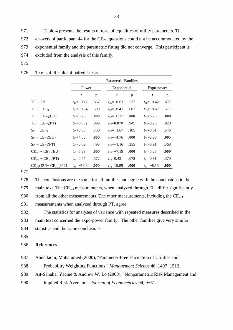
Table 4 presents the results of tests of equalities of utility parameters. The 971

answers of participant 44 for the CE2/3 questions could not be accommodated by the 972

exponential family and the parametric fitting did not converge. This participant is 973

excluded from the analysis of this family. 974

975

TABLE 4. Results of paired t-tests 976

Parametric Families

Power Exponential Expo-power

t p t p t p

TO − SP t46=−0.17 .867 t45=−0.63 .532 t46=−0.42 .677

TO − CE1/3 t33=−0.54 .590 t32=−0.41 .682 t33=−0.67 .511

TO − CE2/3(EU) t33=6.76 .000 t32=−6.27 .000 t33=6.25 .000

TO − CE2/3(PT) t33=0.002 .999 t32=0.070 .945 t33=0.23 .820

SP − CE1/3 t33=0.35 .730 t32=−1.67 .105 t33=0.61 .546

SP − CE2/3(EU) t33=4.05 .000 t32=−4.76 .000 t33=2.98 .005

SP − CE2/3(PT) t33=0.69 .493 t32=−1.16 .255 t33=0.91 .368

CE1/3 − CE2/3(EU) t33=5.23 .000 t32=−7.19 .000 t33=5.27 .000

CE1/3 − CE2/3(PT) t33=0.57 .572 t32=0.43 .672 t33=0.91 .370

CE2/3(EU)− CE2/3(PT) t33=−13.34 .000 t32=10.09 .000 t33=−8.13 .000

977

The conclusions are the same for all families and agree with the conclusions in the 978

main text. The CE2/3 measurements, when analyzed through EU, differ significantly 979

from all the other measurements. The other measurements, including the CE2/3 980

measurements when analyzed through PT, agree. 981

The statistics for analyses of variance with repeated measures described in the 982

main text concerned the expo-power family. The other families give very similar 983

statistics and the same conclusions. 984

985

References 986

Abdellaoui, Mohammed (2000), "Parameter-Free Elicitation of Utilities and 987

Probability Weighting Functions," Management Science 46, 1497−1512. 988

Aït-Sahalia, Yacine & Andrew W. Lo (2000), "Nonparametric Risk Management and 989

Implied Risk Aversion," Journal of Econometrics 94, 9−51. 990

34

Allais, Maurice (1953), "Fondements d'une Théorie Positive des Choix Comportant 991

un Risque et Critique des Postulats et Axiomes de l'Ecole Américaine," 992

Colloques Internationaux du Centre National de la Recherche Scientifique 993

(Econométrie) 40, 257−332. Paris: Centre National de la Recherche Scientifique. 994

Translated into English, with additions, as "The Foundations of a Positive Theory 995

of Choice Involving Risk and a Criticism of the Postulates and Axioms of the 996

American School," in Maurice Allais & Ole Hagen (1979, Eds.), Expected Utility 997

Hypotheses and the Allais Paradox, 27−145, Reidel, Dordrecht, The Netherlands. 998

Alt, Franz (1936), "Über die Messbarkeit des Nutzens." Zeitschrift für 999

Nationalökonomie 7, 161−169. Translated into English by Siegfried Schach 1000

(1971), "On the Measurability of Utility." In John S. Chipman, Leonid Hurwicz, 1001

Marcel K. Richter, & Hugo F. Sonnenschein (Eds.), Preferences, Utility, and 1002

Demand, Hartcourt Brace Jovanovich, New York, Chapter 20. 1003

Arrow, Kenneth J. (1971), "Essays in the Theory of Risk Bearing." North-Holland, 1004

Amsterdam. 1005

Barrios, Carolina (2003), “Une Réconciliation de la Mesure de l’Utilité à l’Aide de la 1006

“Prospect Theory”: Une Approche Experimentale,” Ph.D. dissertation, ENSAM, 1007

Paris, France. 1008

Baumol, William J. (1958), "The Cardinal Utility Which is Ordinal," Economic 1009

Journal 68, 665−672. 1010

Bayoumi, Ahmed & Donald A. Redelmeier (2000), "Decision Analysis with 1011

Cumulative Prospect Theory," Medical Decision Making 20, 404−412. 1012

Bell, David E. (1988), "One-Switch Utility Functions and a Measure of Risk," 1013

Management Science 34, 1416−1424. 1014

Bentham, Jeremy (1789), "The Principles of Morals and Legislation." At the 1015

Clarendom Press, Oxford. 1016

Bernoulli, Daniel (1738), "Specimen Theoriae Novae de Mensura Sortis," 1017

Commentarii Academiae Scientiarum Imperialis Petropolitanae 5, 175−192. 1018

Translated into English by Louise Sommer (1954), "Exposition of a New Theory 1019

on the Measurement of Risk," Econometrica 22, 23−36. 1020

Reprinted in Alfred N. Page (1968, Ed.), Utility Theory: A Book of Readings, 1021

Chapter 11, Wiley, New York. Revised translation in William J. Baumol & 1022

35

Stephen M. Goldfeld (Eds., 1968), Precursors in Mathematical Economics: An 1023

Anthology. Clowes and Sons, London, Selection 2, 15−26. 1024

Binmore, Kenneth G. (1999), "Why Experiments in Economics?," Economic Journal 1025

109, F16−F24. 1026

Binswanger, Hans P. (1981), "Attitudes towards Risk: Theoretical Implications of an 1027

Experiment in Rural India," Economic Journal 91, 867−890. 1028

Birnbaum, Michael H. & Juan B. Navarrete (1998), "Testing Descriptive Utility 1029

Theories: Violations of Stochastic Dominance and Cumulative Independence," 1030

Journal of Risk and Uncertainty 17, 49−78. 1031

Birnbaum, Michael H. & Sara E. Sutton (1992), "Scale Convergence and Utility 1032

Measurement," Organizational Behavior and Human Decision Processes 52, 1033

183−215. 1034

Blaug, Mark (1962), "Economic Theory in Retrospect." Cambridge University Press, 1035

Cambridge. (5th ed. 1997) 1036

Bleichrodt, Han (2002), "A New Explanation for the Difference between SG and TTO 1037

Utilities," Health Economics 11, 447−456. 1038

Bleichrodt, Han & José Luis Pinto (2000), "A Parameter-Free Elicitation of the 1039

Probability Weighting Function in Medical Decision Analysis," Management 1040

Science 46, 1485−1496. 1041

Bleichrodt, Han, José Luis Pinto, & Peter P. Wakker (2001), "Making Descriptive 1042

Use of Prospect Theory to Improve the Prescriptive Use of Expected Utility," 1043

Management Science 47, 1498−1514. 1044

Bliss, Robert R. & Nikolaos Panigirtzoglou (2004), "Option-Implied Risk Aversion 1045

Estimates," Journal of Finance 59, 407−446. 1046

Bostic, Raphael, Richard J. Herrnstein, & R. Duncan Luce (1990), "The Effect on the 1047

Preference-Reversal Phenomenon of Using Choice Indifferences," Journal of 1048

Economic Behavior and Organization 13, 193−212. 1049

Bouyssou, Denis & Jean-Claude Vansnick (1988), "A Note on the Relationships 1050

between Utility and Value Functions." In Bertrand R. Munier (Ed.), Risk, 1051

Decision and Rationality, 103−114, Reidel, Dordrecht, The Netherlands. 1052

Breiter, Hans C., Ithak Aharon, Daniel Kahneman, Anders Dale, & Peter Shizgal 1053

(2001), "Functional Imaging of Neural Responses to Expectancy and Experience 1054

of Monetary Gains and Losses," Neuron 30, 619−639. 1055

36

Broome, John R. (1991), "Weighing Goods." Basil Blackwell, Oxford, UK. 1056

Camerer, Colin F. (1995), "Individual Decision Making." In John H. Kagel & Alvin 1057

E. Roth (Eds.), Handbook of Experimental Economics, 587−703, Princeton 1058

University Press, Princeton, NJ. 1059

Camerer, Colin F. & Teck-Hua Ho (1994), "Violations of the Betweenness Axiom 1060

and Nonlinearity in Probability," Journal of Risk and Uncertainty 8, 167−196. 1061

Camerer, Colin F. & Robin M. Hogarth (1999), "The Effects of Financial Incentives 1062

in Experiments: A Review and Capital-Labor-Production Framework," Journal of 1063

Risk and Uncertainty 19, 7−42. 1064

Cooter, Robert D. & Peter Rappoport (1984), "Were the Ordinalists Wrong about 1065

Welfare Economics?," Journal of Economic Literature 22, 507−530. 1066

Cramer, Gabriel (1728), Letter from Cramer to Nicholas Bernoulli. Translated into 1067

English by Louise Sommer in Bernoulli, Daniel (1954), "Exposition of a New 1068

Theory on the Measurement of Risk," Econometrica 22, 23−36. 1069

Debreu, Gérard (1959), "Cardinal Utility for Even-Chance Mixtures of Pairs of Sure-1070

Prospects," Review of Economic Studies 26, 174−177. 1071

Debreu, Gérard (1976), "Least Concave Utility Functions," Journal of Mathematical 1072

Economics 3, 121−129. 1073

Edgeworth, F. Ysidro (1881), "Mathematical Physics, An Essay on the Application of 1074

Mathematics to the Moral Sciences." 1075

Reprinted 1967, M. Kelley, New York. 1076

Ellingsen, Tore (1994), "Cardinal Utility: A History of Hedinometry." In Maurice 1077

Allais & Ole Hagen (Eds.), Cardinalism; A Fundamental Approach, 105−165, 1078

Kluwer Academic Publishers, Dordrecht, The Netherlands. 1079

Ellsberg, Daniel (1954), "Classic and Current Notions of 'Measurable Utility'," 1080

Economic Journal 62, 528−556. 1081

Ellsberg, Daniel (1961), "Risk, Ambiguity and the Savage Axioms," Quarterly 1082

Journal of Economics 75, 643−669. 1083

Farquhar, Peter H. & Yutaka Nakamura (1987), "Constant Exchange Risk Properties," 1084

Operations Research 35, 206−214. 1085

Fellner, Wiliam (1961), "Distortion of Subjective Probabilities as a Reaction to 1086

Uncertainty," Quarterly Journal of Economics 75, 670−689. 1087

37

Fishburn, Peter C. (1978), "On Handa's "New Theory of Cardinal Utility" and the 1088

Maximization of Expected Return," Journal of Political Economy 86, 321−324. 1089

Frey, Bruno S. & Felix Oberholzer-Gee (1997), "The Cost of Price Incentives: An 1090

Empirical Analysis of Motivation Crowding-Out," American Economic Review 1091

87, 746−755. 1092

Frey, Bruno S. & Alois Stutzer (2000), "Happiness, Economy and Institutions," 1093

Economic Journal 110, 918−938. 1094

Friedman, Milton & Leonard J. Savage (1948), "The Utility Analysis of Choices 1095

Involving Risk," Journal of Political Economy 56, 279−304. 1096

Frisch, Ragnar (1926), "Sur un Problème d'Economie Pure," Norsk Matematisk 1097

Forenings Skrifter Serie 1 16, 1−40. Translated into English by John S. 1098

Chipman, "On a Problem in Pure Economics." In John S. Chipman, Leonid 1099

Hurwicz, Marcel K. Richter, & Hugo F. Sonnenschein (1971, Eds.), Preferences, 1100

Utility, and Demand, Chapter 19, Hartcourt, New York. 1101

Gilboa, Itzhak (1987), "Expected Utility with Purely Subjective Non-Additive 1102

Probabilities," Journal of Mathematical Economics 16, 65−88. 1103

Gilboa, Itzhak & David Schmeidler (1995), "Case-Based Decision Theory," Quarterly 1104

Journal of Economics 110, 605−639. 1105

Gilboa, Itzhak & David Schmeidler (2001), "A Cognitive Model of Individual Well-1106

Being," Social Choice and Welfare 18, 269−288. 1107

Gneezy, Uri, & Aldo Rustichini (2000), "Pay Enough or Don’t Pay at All," Quarterly 1108

Journal of Economics 115, 791−810. 1109

Gold, Marthe R., Joanna E. Siegel, Louise B. Russell, & Milton C. Weinstein (1996), 1110

"Cost-Effectiveness in Health and Medicine." Oxford University Press, New 1111

York. 1112

Gonzalez, Richard & George Wu (1999), "On the Shape of the Probability Weighting 1113

Function," Cognitive Psychology 38, 129−166. 1114

Gregory, Allen W., Jean-François Lamarche, & Gregor W. Smith (2002), 1115

"Information-Theoretic Estimation of Preference Parameters: Macroeconomic 1116

Applications and Simulation Evidence," Journal of Econometrics 107, 213−233. 1117

Gregory, Robin, Sarah Lichtenstein, & Paul Slovic (1993), "Valuing Environmental 1118

Resources: A Constructive Approach," Journal of Risk and Uncertainty 7, 1119

177−197. 1120

38

Grether, David M. & Charles R. Plott (1979), "Economic Theory of Choice and the 1121

Preference Reversal Phenomenon," American Economic Review 69, 623−638. 1122

Gul, Faruk (1991), "A Theory of Disappointment Aversion," Econometrica 59, 1123

667−686. 1124

Handa, Jagdish (1977), "Risk, Probabilities, and a New Theory of Cardinal Utility," 1125

Journal of Political Economy 85, 97−122. 1126

Harbaugh, William T., Kate Krause, & Lise Vesterlund (2001), "Prospect Theory in 1127

Choice and Pricing Tasks," 1128

Harsanyi, John C. (1955), "Cardinal Welfare, Individualistic Ethics, and Interpersonal 1129

Comparisons of Utility," Journal of Political Economy 63, 309−321. 1130

Hershey, John C. & Paul J.H. Schoemaker (1985), "Probability versus Certainty 1131

Equivalence Methods in Utility Measurement: Are They Equivalent?," 1132

Management Science 31, 1213−1231. 1133

Hertwig, Ralf & Andreas Ortmann (2001), "Experimental Practices In Economics: A 1134

Challenge for Psychologists?," Behavioral and Brain Sciences 24, 383−403. 1135

Hicks, John R. & Roy G.D. Allen (1934), "A Reconsideration of the Theory of Value: 1136

I; II," Economica 1, 52−75; 196−219. 1137

Houthakker, Hendrik S. (1950), "Revealed Preference and the Utility Function," 1138

Economica, N.S. 17, 159−174. 1139

Kachelmeier, Steven J. & Mohamed Shehata (1992), "Examining Risk Preferences 1140

under High Monetary Incentives: Experimental Evidence from the People's 1141

Republic of China," American Economic Review 82, 1120−1141; for comment 1142

see Steven J. Kachelmeier & Mohammed Shehata (1994), American Economic 1143

Review 84, 1104−1106. 1144

Kahneman, Daniel (1994), "New Challenges to the Rationality Assumption," Journal 1145

of Institutional and Theoretical Economics 150, 18−36. 1146

Kahneman, Daniel & Amos Tversky (1979), "Prospect Theory: An Analysis of 1147

Decision under Risk," Econometrica 47, 263−291. 1148

Kahneman, Daniel & Amos Tversky (2000, Eds.), "Choices, Values, and Frames." 1149

Cambridge University Press, New York. 1150

Kapteyn, Arie (1994), "The Measurement of Household Cost Functions: Revealed 1151

Preference versus Subjective Measures," Journal of Population Economics 7, 1152

333−350. 1153

39

Karmarkar, Uday S. (1978), "Subjectively Weighted Utility: A Descriptive Extension 1154

of the Expected Utility Model," Organizational Behavior and Human 1155

Performance 21, 61−72. 1156

Karni, Edi & Zvi Safra (1990), "Rank-Dependent Probabilities," Economic Journal 1157

100, 487−495. 1158

Krzysztofowicz, Roman & John B. Koch (1989), "Estimation of Cardinal Utility 1159

Based on a Nonlinear Theory," Annals of Operations Research 19, 181−204. 1160

Lichtenstein, Sarah & Paul Slovic (1971), "Reversals of Preference between Bids and 1161

Choices in Gambling Decisions," Journal of Experimental Psychology 89, 46−55. 1162

Loewenstein, George F. (1999), "Experimental Economics from the Vantage-Point of 1163

Behavioural Economics," Economic Journal 109, F25−F34. 1164

Loomes, Graham & Robert Sugden (1982), "Regret Theory: An Alternative Theory of 1165

Rational Choice under Uncertainty," Economic Journal 92, 805−824. 1166

Loomes, Graham, Chris Starmer, & Robert Sugden (2003), "Do Anomalies Disappear 1167

in Repeated Markets?," The Economic Journal 113, C153−C166. 1168

Machina, Mark J. (1982), " 'Expected Utility' Analysis without the Independence 1169

Axiom," Econometrica 50, 277−323. 1170

Manski, Charles F. (2004), "Measuring Expectations," Econometrica 72, 1329−1376. 1171

Marshall, Alfred (1890), "Principles of Economics." 8th edition 1920 (9th edition 1172

1961), MacMillan, New York. 1173

McCord, Mark R. & Richard de Neufville (1983), "Fundamental Deficiency of 1174

Expected Utility Decision Analysis." In Simon French, R. Hartley, L.C. Thomas, 1175

& Douglas J. White (Eds.), Multi-Objective Decision Making, 279−305, 1176

Academic Press, New York. 1177

McCord, Mark R. & Richard de Neufville (1984), "Utility Dependence on 1178

Probability: An Empirical Demonstration," Large Scale Systems 6, 91−103. 1179

McCord, Mark R. & Richard de Neufville (1986), " "Lottery Equivalents ": Reduction 1180

of the Certainty Effect Problem in Utility Assessment," Management Science 32, 1181

56−60. 1182

Merton, Robert C. (1971), "Optimum Consumption and Portfolio Rules in a 1183

Continuous-Time Model," Journal of Economic Theory 3, 373−413. 1184

Nakamura, Yutaka (1996), "Sumex Utility Functions," Mathematical Social Sciences 1185

31, 39−47. 1186

40

Ng, Yew-Kwang (1997), "A Case for Happiness, Cardinalism, and Interpersonal 1187

Comparability," Economic Journal 107, 1848−1858. 1188

Pareto, Vilfredo (1906), "Manuele di Economia Politica." Piccolo Biblioteca 1189

Scientifica, Milan. Translated into English by Ann S. Schwier (1971), "Manuel of 1190

Political Economy," MacMillan, London. 1191

Translated into French in 1927 as "Manuel d'Economie Politique." Giard, Paris, 1192

second edition. 1193

Pennings, Joost M.E. & Ale Smidts (2000), "Assessing the Construct Validity of Risk 1194

Attitude," Management Science 46, 1337−1348. 1195

Perraudin, William R.M. & Bent E. Sorensen (2000), "The Demand for Risky Assets: 1196

Sample Selection and Household Portfolios," Journal of Econometrics 97, 1197

117−144. 1198

Prelec, Drazen (1998), "The Probability Weighting Function," Econometrica 66, 1199

497−527. 1200

Quiggin, John (1982), "A Theory of Anticipated Utility," Journal of Economic 1201

Behaviour and Organization 3, 323−343. 1202

Rabin, Matthew (2000), "Risk Aversion and Expected-utility Theory: A Calibration 1203

Theorem," Econometrica 68, 1281−1292. 1204

Ramsey, Frank P. (1931), "Truth and Probability." In "The Foundations of 1205

Mathematics and other Logical Essays," 156−198, Routledge and Kegan Paul, 1206

London. 1207

Reprinted in Henry E. Kyburg Jr. & Howard E. Smokler (1964, Eds.), Studies in 1208

Subjective Probability, 61−92, Wiley, New York. (2nd edition 1980, Krieger, 1209

New York.) 1210

Revicki, Dennis A. & Robert M. Kaplan (1993), "Relationship between Psychometric 1211

and Utility-Based Approaches to the Measurement of Health-Related Quality of 1212

Life," Quality Life Research 2, 477−487. 1213

Robinson, Angela, Graham Loomes, & Michael Jones-Lee (2001), "Visual Analog 1214

Scales, Standard Gambles, and Relative Risk Aversion," Medical Decision 1215

Making 21, 17−21. 1216

Robson, Arthur J. (2001), "Why Would Nature Give Individuals Utility Functions?," 1217

The Journal of Political Economy 109, 900−914. 1218

41

Saha, Atanu (1993), "Expo-power Utility: A Flexible Form for Absolute and Relative 1219

Aversion," American Journal of Agricultural Economics 75, 905−913. 1220

Samuelson, Paul A. (1937), "A Note on Measurement of Utility," Review of Economic 1221

Studies 4 (issue 2, February 1937), 155−161. 1222

Samuelson, Paul A. (1938a), "The Numerical Representation of Ordered 1223

Classifications and the Concept of Utility," Review of Economic Studies 6 (Issue 1224

1, October 1938), 65–70. 1225

Samuelson, Paul A. (1938b), "A Note on the Pure Theory of Consumer's Behaviour," 1226

Economica, N.S. 5, 61−71, 353−354. 1227

Samuelson, Paul A. (1950), "The Problem of Integrability in Utility Theory," 1228

Economica, N.S. 17, 355−385. 1229

Savage, Leonard J. (1954), "The Foundations of Statistics." Wiley, New York. 1230

(Second edition 1972, Dover Publications, New York.) 1231

Schmeidler, David (1989), "Subjective Probability and Expected Utility without 1232

Additivity," Econometrica 57, 571−587. 1233

Sen, Amartya K. (1974), "Informational Bases of Alternative Welfare Approaches. 1234

Aggregation and Income Distribution," Journal of Public Economics 3, 387−403. 1235

Shafir, Eldar, Peter A. Diamond, & Amos Tversky (1997), "Money Illusion," 1236

Quarterly Journal of Economics 112, 341−374. 1237

Simon, Herbert A. (1955), "A Behavioral Model of Rational Choice," Quarterly 1238

Journal of Economics 69, 99−118. 1239

Skinner, Burrhus F. (1971), "Beyond Freedom and Dignity." Knopf, N.Y. 1240

Smith, Vernon L. (1982), "Microeconomic Systems as an Experimental Science," 1241

American Economic Review 72, 923−955. 1242

Starmer, Chris (2000), "Developments in Non-Expected Utility Theory: The Hunt for 1243

a Descriptive Theory of Choice under Risk," Journal of Economic Literature 38, 1244

332−382. 1245

Stigler, George J. (1950), "The Development of Utility Theory: I; II," Journal of 1246

Political Economy 58, 307−327; 373−396. 1247

Reprinted in Alfred N. Page (1968), Utility Theory: A Book of Readings, Wiley, 1248

New York, 55−119. 1249

Tinbergen, Jan (1991), "On the Measurement of Welfare," Journal of Econometrics 1250

50, 7−13. 1251

42

Torrance, George W., Michael H. Boyle, & Sargent P. Horwood (1982), "Application 1252

of Multi-Attribute Utility Theory to Measure Social Preferences for Health 1253

States," Operations Research 30, 1043−1069. 1254

Tversky, Amos & Craig R. Fox (1995), "Weighing Risk and Uncertainty," 1255

Psychological Review 102, 269−283. 1256

Tversky, Amos & Daniel Kahneman (1992), "Advances in Prospect Theory: 1257

Cumulative Representation of Uncertainty," Journal of Risk and Uncertainty 5, 1258

297−323. 1259

van Praag, Bernard M.S. (1968), "Individual Welfare Functions and Consumer 1260

Behavior." North-Holland, Amsterdam, 1968. 1261

Van Praag, Bernard M.S. (1991), "Ordinal and Cardinal Utility: An Integration of the 1262

Two Dimensions of the Welfare Concept," Journal of Econometrics 50, 69−89. 1263

Van Soest, Arthur, Marcel Das, & Xiaodong Gong (2005), "A Structural Labour 1264

Supply Model with Flexible Preferences," Journal of Econometrics 107, 1265

345−374. 1266

Varian, Hal R. (1993), "Intermediate Microeconomics." Norton, New York. 1267

von Neumann, John & Oskar Morgenstern (1944, 1947, 1953), "Theory of Games and 1268

Economic Behavior." Princeton University Press, Princeton NJ. 1269

von Winterfeldt, Detlof & Ward Edwards (1986), "Decision Analysis and Behavioral 1270

Research." Cambridge University Press, Cambridge, UK. 1271

Wakker, Peter P. & Daniel Deneffe (1996), "Eliciting von Neumann-Morgenstern 1272

Utilities when Probabilities Are Distorted or Unknown," Management Science 1273

42, 1131−1150. 1274

Wakker, Peter P. & Anne M. Stiggelbout (1995), "Explaining Distortions in Utility 1275

Elicitation through the Rank-Dependent Model for Risky Choices," Medical 1276

Decision Making 15, 180−186. 1277

Watson, John B. (1913), "Psychology as the Behaviorist Views It," Psychological 1278

Review 20, 158−177. 1279

Weber, Elke U. (1994), "From Subjective Probabilities to Decision Weights: The 1280

Effects of Asymmetric Loss Functions on the Evaluation of Uncertain Outcomes 1281

and Events," Psychological Bulletin 115, 228−242. 1282

Yaari, Menahem E. (1965), "Convexity in the Theory of Choice under Risk," 1283

Quarterly Journal of Economics 79, 278−290. 1284

43

Yaari, Menahem E. (1987), "The Dual Theory of Choice under Risk," Econometrica 1285

55, 95−115. 1286

Zellner, Arnold (1971), An Introduction to Bayesian Inference in Econometrics. 1287

Wiley, New York. 1288

Zeuthen, Frederik (1937), "On the Determinateness of the Utility Function," Review 1289

of Economic Studies 4, 236−239. 1290

Köbberling & Wakker waar? 1291