Chapter 9Recommendation in Social Media

This chapter is from Social Media Mining: An Introduction.By Reza Zafarani, Mohammad Ali Abbasi, and Huan Liu.Cambridge University Press, 2014. Draft version: April 20, 2014.Complete Draft and Slides Available at: http://dmml.asu.edu/smm

Individuals in social media make a variety of decisions on a daily basis.These decisions are about buying a product, purchasing a service, addinga friend, and renting a movie, among others. The individual often facesmany options to choose from. These diverse options, the pursuit of opti-mality, and the limited knowledge that each individual has create a desirefor external help. At times, we resort to search engines for recommen-dations; however, the results in search engines are rarely tailored to ourparticular tastes and are query-dependent, independent of the individualswho search for them.

Applications and algorithms are developed to help individuals de-cide easily, rapidly, and more accurately. These algorithms are tailoredto individuals’ tastes such that customized recommendations are avail-able for them. These algorithms are called recommendation algorithms orrecommender systems.

Recommender System

Recommender systems are commonly used for product recommenda-tion. Their goal is to recommend products that would be interesting toindividuals. Formally, a recommendation algorithm takes a set of users Uand a set of items I and learns a function f such that

f : U × I→ R (9.1)

In other words, the algorithm learns a function that assigns a real valueto each user-item pair (u, i), where this value indicates how interested useru is in item i. This value denotes the rating given by user u to item i. Therecommendation algorithm is not limited to item recommendation and

289

can be generalized to recommending people and material, such as, ads orcontent.

Recommendation vs. Search

When individuals seek recommendations, they often use web search en-gines. However, search engines are rarely tailored to individuals’ needsand often retrieve the same results as long as the search query stays thesame. To receive accurate recommendation from a search engine, oneneeds to send accurate keywords to the search engine. For instance, thequery ‘‘best 2013 movie to watch’’ issued by an 8-year old and anadult will result in the same set of movies, whereas their individual tastesdictate different movies.

Recommendation systems are designed to recommend individual-basedchoices. Thus, the same query issued by different individuals should resultin different recommendations. These systems commonly employ browsinghistory, product purchases, user profile information, and friends informa-tion to make customized recommendations. As simple as this process maylook, a recommendation system algorithm actually has to deal with manychallenges.

9.1 Challenges

Recommendation systems face many challenges, some of which are pre-sented next:

• Cold-Start Problem. Many recommendation systems use histori-cal data or information provided by the user to recommend items,products, and the like. However, when individuals first join sites,they have not yet bought any product: they have no history. Thismakes it hard to infer what they are going to like when they starton a site. The problem is referred to as the cold-start problem. Asan example, consider an online movie rental store. This store has noidea what recently joined users prefer to watch and therefore cannotrecommend something close to their tastes. To address this issue,these sites often ask users to rate a couple of movies before they be-gin recommend others to them. Other sites ask users to fill in profile

290

information, such as interests. This information serves as an input tothe recommendation algorithm.

• Data Sparsity. Similar to the cold-start problem, data sparsity occurswhen not enough historical or prior information is available. Un-like the cold-start problem, data sparsity relates to the system as awhole and is not specific to an individual. In general, data sparsityoccurs when a few individuals rate many items while many otherindividuals rate only a few items. Recommender systems often useinformation provided by other users to help offer better recommen-dations to an individual. When this information is not reasonablyavailable, then it is said that a data sparsity problem exists. The prob-lem is more promi- nent in sites that are recently launched or onesthat are not popular.

• Attacks. The recommender system may be attacked to recommenditems otherwise not recommended. For instance, consider a systemthat recommends items based on similarity between ratings (e.g.,lens A is recommended for camera B because they both have rating4). Now, an attacker that has knowledge of the recommendationalgorithm can create a set of fake user accounts and rate lens C (whichis not as good as lens A) highly such that it can get rating 4. Thisway the recommendation system will recommend C with camera Bas well as A. This attack is called a push attack, because it pushes Nuke Attack

andPush Attack

the ratings up such that the system starts recommending items thatwould otherwise not be recommended. Other attacks such as nukeattacks attempt to stop the whole recommendation system algorithmand make it unstable. A recommendation system should have themeans to stop such attacks.

• Privacy. The more information a recommender system has aboutthe users, the better the recommendations it provides to the users.However, users often avoid revealing information about themselvesdue to privacy concerns. Recommender systems should address thischallenge while protecting individuals’ privacy.

• Explanation. Recommendation systems often recommend itemswithout having an explanation why they did so. For instance, when

291

several items are bought together by many users, the system recom-mends these to new users items together. However, the system doesnot know why these items are bought together. Individuals mayprefer some reasons for buying items; therefore, recommendationalgorithms should provide explanation when possible.

9.2 Classical Recommendation Algorithms

Classical recommendation algorithms have a long history on the web. Inrecent years, with the emergence of social media sites, these algorithmshave been provided new information, such as friendship information, in-teractions, and so on. We review these algorithms in this section.

9.2.1 Content-Based Methods

Content-based recommendation systems are based on the fact that a user’sinterest should match the description of the items that are recommendedby the system. In other words, the more similar the item’s descriptionto the user’s interest, the higher the likelihood that the user is going tofind the item’s recommendation interesting. Content-based recommendersystems implement this idea by measuring the similarity between an item’sdescription and the user’s profile information. The higher this similarity,the higher the chance that the item is recommended.

To formalize a content-based method, we first represent both user pro-files and item descriptions by vectorizing (see Chapter 5) them using aset of k keywords. After vectorization, item j can be represented as a k-dimensional vector I j = (i j,1, i j,2, . . . , i j,k) and user i as Ui = (ui,1,ui,2, . . . ,ui,k).To compute the similarity between user i and item j, we can use cosinesimilarity between the two vectors Ui and I j:

sim(Ui, I j) = cos(Ui, I j) =

∑kl=1 ui,li j,l√∑k

l=1 ui,l2√∑k

l=1 i j,l2

(9.2)

In content-based recommendation, we compute the topmost similaritems to a user j and then recommend these items in the order of similarity.Algorithm 9.1 shows the main steps of content-based recommendation.

292

Algorithm 9.1 Content-based recommendationRequire: User i’s Profile Information, Item descriptions for items j ∈{1, 2, . . . ,n}, k keywords, r number of recommendations.

1: return r recommended items.2: Ui = (u1,u2, . . . ,uk) = user i’s profile vector;3: {I j}

nj=1 = {(i j,1, i j,2, . . . , i j,k) = item j’s description vector}nj=1;

4: si, j = sim(Ui, I j), 1 ≤ j ≤ n;5: Return top r items with maximum similarity si, j.

Table 9.1: User-Item Matrix

Lion King Aladdin Mulan AnastasiaJohn 3 0 3 3Joe 5 4 0 2Jill 1 2 4 2Jane 3 ? 1 0Jorge 2 2 0 1

9.2.2 Collaborative Filtering (CF)

Collaborative filtering is another set of classical recommendation tech-niques. In collaborative filtering, one is commonly given a user-item ma-trix where each entry is either unknown or is the rating assigned by theuser to an item. Table 9.1 is an user-item matrix where ratings for some car-toons are known and unknown for others (question marks). For instance,on a review scale of 5, where 5 is the best and 0 is the worst, if an entry (i, j)in the user-item matrix is 4, that means that user i liked item j.

In collaborative filtering, one aims to predict the missing ratings andpossibly recommend the cartoon with the highest predicted rating to theuser. This prediction can be performed directly by using previous ratingsin the matrix. This approach is called memory-based collaborative filteringbecause it employs historical data available in the matrix. Alternatively,one can assume that an underlying model (hypothesis) governs the wayusers rate items. This model can be approximated and learned. Afterthe model is learned, one can use it to predict other ratings. The secondapproach is called model-based collaborative filtering.

293

Memory-Based Collaborative Filtering

In memory-based collaborative filtering, one assumes one of the following(or both) to be true:

• Users with similar previous ratings for items are likely to rate futureitems similarly.

• Items that have received similar ratings previously from users arelikely to receive similar ratings from future users.

If one follows the first assumption, the memory-based technique is auser-based CF algorithm, and if one follows the latter, it is an item-basedCF algorithm. In both cases, users (or items) collaboratively help filterout irrelevant content (dissimilar users or items). To determine similaritybetween users or items, in collaborative filtering, two commonly usedsimilarity measures are cosine similarity and Pearson correlation. Let ru,i

denote the rating that user u assigns to item i, let r̄u denote the averagerating for user u, and let r̄i be the average rating for item i. Cosine similaritybetween users u and v is

sim(Uu,Uv) = cos(Uu,Uv) =Uu ·Uv

||Uu|| ||Uv||=

∑i ru,irv,i√∑

i ru,i2√∑

i rv,i2. (9.3)

And the Pearson correlation coefficient is defined as

sim(Uu,Uv) =

∑i (ru,i − r̄u)(rv,i − r̄v)√∑

i (ru,i − r̄u)2√∑

i (rv,i − r̄v)2. (9.4)

Next, we discuss user- and item-based collaborative filtering.User-Based Collaborative Filtering. In this method, we predict the ratingof user u for item i by (1) finding users most similar to u and (2) usinga combination of the ratings of these users for item i as the predictedrating of user u for item i. To remove noise and reduce computation, weoften limit the number of similar users to some fixed number. These mostsimilar users are called the neighborhood for user u, N(u). In user-basedNeighborhoodcollaborative filtering, the rating of user u for item i is calculated as

ru,i = r̄u +

∑v∈N(u) sim(u, v)(rv,i − r̄v)∑

v∈N(u) sim(u, v), (9.5)

where the number of members of N(u) is predetermined (e.g., top 10 mostsimilar members).

294

Example 9.1. In Table 9.1, rJane,Aladdin is missing. The average ratings are thefollowing:

r̄John =3 + 3 + 0 + 3

4= 2.25 (9.6)

r̄Joe =5 + 4 + 0 + 2

4= 2.75 (9.7)

r̄Jill =1 + 2 + 4 + 2

4= 2.25 (9.8)

r̄Jane =3 + 1 + 0

3= 1.33 (9.9)

r̄Jorge =2 + 2 + 0 + 1

4= 1.25. (9.10)

Using cosine similarity (or Pearson correlation), the similarity between Janeand others can be computed:

sim(Jane, John) =3× 3 + 1× 3 + 0× 3

√10√

27= 0.73 (9.11)

sim(Jane, Joe) =3× 5 + 1× 0 + 0× 2

√10√

29= 0.88 (9.12)

sim(Jane, Jill) =3× 1 + 1× 4 + 0× 2

√10√

21= 0.48 (9.13)

sim(Jane, Jorge) =3× 2 + 1× 0 + 0× 1

√10√

5= 0.84. (9.14)

Now, assuming that the neighborhood size is 2, then Jorge and Joe are the twomost similar neighbors. Then, Jane’s rating for Aladdin computed from user-basedcollaborative filtering is

rJane,Aladdin = r̄Jane +sim(Jane, Joe)(rJoe,Aladdin − r̄Joe)

sim(Jane, Joe) + sim(Jane, Jorge)

+sim(Jane, Jorge)(rJorge,Aladdin − r̄Jorge)

sim(Jane, Joe) + sim(Jane, Jorge)

= 1.33 +0.88(4 − 2.75) + 0.84(2 − 1.25)

0.88 + 0.84= 2.33 (9.15)

295

Item-based Collaborative Filtering. In user-based collaborative filtering,we compute the average rating for different users and find the most similarusers to the users for whom we are seeking recommendations. Unfortu-nately, in most online systems, users do not have many ratings; therefore,the averages and similarities may be unreliable. This often results in a dif-ferent set of similar users when new ratings are added to the system. Onthe other hand, products usually have many ratings and their average andthe similarity between them are more stable. In item-based CF, we performcollaborative filtering by finding the most similar items. The rating of useru for item i is calculated as

ru,i = r̄i +

∑j∈N(i) sim(i, j)(ru, j − r̄ j)∑

j∈N(i) sim(i, j), (9.16)

where r̄i and r̄ j are the average ratings for items i and j, respectively.

Example 9.2. In Table 9.1, rJane,Aladdin is missing. The average ratings for itemsare

r̄Lion King =3 + 5 + 1 + 3 + 2

5= 2.8. (9.17)

r̄Aladdin =0 + 4 + 2 + 2

4= 2. (9.18)

r̄Mulan =3 + 0 + 4 + 1 + 0

5= 1.6. (9.19)

r̄Anastasia =3 + 2 + 2 + 0 + 1

5= 1.6. (9.20)

Using cosine similarity (or Pearson correlation), the similarity between Al-addin and others can be computed:

sim(Aladdin,Lion King) =0 × 3 + 4 × 5 + 2 × 1 + 2 × 2

√24√

39= 0.84.

(9.21)

sim(Aladdin,Mulan) =0 × 3 + 4 × 0 + 2 × 4 + 2 × 0

√24√

25= 0.32.

(9.22)

sim(Aladdin,Anastasia) =0 × 3 + 4 × 2 + 2 × 2 + 2 × 1

√24√

18= 0.67.

(9.23)

296

Now, assuming that the neighborhood size is 2, then Lion King and Anastasiaare the two most similar neighbors. Then, Jane’s rating for Aladdin computedfrom item-based collaborative filtering is

rJane,Aladdin = r̄Aladdin+sim(Aladdin,Lion King)(rJane,Lion King − r̄Lion King)

sim(Aladdin,Lion King) + sim(Aladdin,Anastasia)

+sim(Aladdin,Anastasia)(rJane,Anastasia − r̄Anastasia)

sim(Aladdin,Lion King) + sim(Aladdin,Anastasia)

= 2 +0.84(3 − 2.8) + 0.67(0 − 1.6)

0.84 + 0.67= 1.40. (9.24)

Model-Based Collaborative Filtering

In memory-based methods (either item-based or user-based), one aims topredict the missing ratings based on similarities between users or items. Inmodel-based collaborative filtering, one assumes that an underlying modelgoverns the way users rate. We aim to learn that model and then use thatmodel to predict the missing ratings. Among a variety of model-basedtechniques, we focus on a well-established model-based technique that isbased on singular value decomposition (SVD). Singular

ValueDecomposition

SVD is a linear algebra technique that, given a real matrix X ∈ Rm×n,m ≥ n, factorizes it into three matrices,

X = UΣVT, (9.25)

where U ∈ Rm×m and V ∈ Rn×n are orthogonal matrices and Σ ∈ Rm×n is adiagonal matrix. The product of these matrices is equivalent to the originalmatrix; therefore, no information is lost. Hence, the process is lossless.

LosslessMatrixFactorization

Let ‖X‖F =√∑m

i=1∑n

j=1 X2i j denote the Frobenius norm of matrix X. A

low-rank matrix approximation of matrix X is another matrix C ∈ Rm×n. Capproximates X, and C’s rank (the maximum number of linearly indepen-dent columns) is a fixed number k� min(m,n):

FrobeniusNorm

rank(C) = k. (9.26)

The best low-rank matrix approximation is a matrix C that minimizes‖X−C‖F. Low-rank approximations of matrices remove noise by assumingthat the matrix is not generated at random and has an underlying structure.

297

SVD can help remove noise by computing a low-rank approximation of amatrix. Consider the following matrix Xk, which we construct from matrixX after computing the SVD of X = UΣVT:

1. Create Σk from Σ by keeping only the first k elements on the diagonal.This way, Σk ∈ Rk×k.

2. Keep only the first k columns of U and denote it as Uk ∈ Rm×k, andkeep only the first k rows of VT and denote it as Vk

T∈ Rk×n.

3. Let Xk = UkΣkVkT, Xk ∈ Rm×n.

As it turns out, Xk is the best low-rank approximation of a matrix X. Thefollowing Eckart-Young-Mirsky theorem outlines this result.

Eckart-Young-MirskyTheorem

Theorem 9.1 (Eckart-Young-Mirsky Low-Rank Matrix Approximation).Let X be a matrix and C be the best low-rank approximation of X; if ‖X − C‖F isminimized, and rank(C) = k, then C = Xk.

To summarize, the best rank-k approximation of the matrix can be easilycomputed by calculating the SVD of the matrix and then taking the first kcolumns of U, truncating Σ to the the first k entries, and taking the first krows of VT.

As mentioned, low-rank approximation helps remove noise from amatrix by assuming that the matrix is low rank. In low-rank approximationusing SVD, if X ∈ Rm×n, then Uk ∈ Rm×k, Σk ∈ Rk×k, and VT

k ∈ Rk×n.

Hence, Uk has the same number of rows as X, but in a k-dimensional space.Therefore, Uk represents rows of X, but in a transformed k-dimensionalspace. The same holds for VT

k because it has the same number of columnsas X, but in a k-dimensional space. To summarize, Uk and VT

k can bethought of as k-dimensional representations of rows and columns of X. Inthis k-dimensional space, noise is removed and more similar points shouldbe closer.

Now, given the user-item matrix X, we can remove its noise by com-puting Xk from X and getting the new k-dimensional user space Uk or thek-dimensional item space VT

k . This way, we can compute the most similarneighbors based on distances in this k-dimensional space. The similarityin the k-dimensional space can be computed using cosine similarity orPearson correlation. We demonstrate this via Example 9.3.

298

Table 9.2: An User-Item MatrixLion King Aladdin Mulan

John 3 0 3Joe 5 4 0Jill 1 2 4Jorge 2 2 0

Example 9.3. Consider the user-item matrix, in Table 9.2. Assuming this matrixis X, then by computing the SVD of X = UΣVT,1 we have

U =

−0.4151 −0.4754 −0.7679 0.1093−0.7437 0.5278 0.0169 −0.4099−0.4110 −0.6626 0.6207 −0.0820−0.3251 0.2373 0.1572 0.9018

(9.27)

Σ =

8.0265 0 0

0 4.3886 00 0 2.07770 0 0

(9.28)

VT =

−0.7506 −0.5540 −0.36000.2335 0.2872 −0.9290−0.6181 0.7814 0.0863

(9.29)

Considering a rank 2 approximation (i.e., k = 2), we truncate all three matrices:

Uk =

−0.4151 −0.4754−0.7437 0.5278−0.4110 −0.6626−0.3251 0.2373

(9.30)

Σk =

[8.0265 0

0 4.3886

](9.31)

VTk =

[−0.7506 −0.5540 −0.3600

0.2335 0.2872 −0.9290

]. (9.32)

The rows of Uk represent users. Similarly the columns of VTk (or rows of Vk)

represent items. Thus, we can plot users and items in a 2-D figure. By plotting

1In Matlab, this can be performed using the svd command.

299

Figure 9.1: Users and Items in the 2-D Space.

user rows or item columns, we avoid computing distances between them and canvisually inspect items or users that are most similar to one another. Figure 9.1depicts users and items depicted in a 2-D space. As shown, to recommend for Jill,John is the most similar individual to her. Similarly, the most similar item to LionKing is Aladdin.

After most similar items or users are found in the lower k-dimensionalspace, one can follow the same process outlined in user-based or item-based collaborative filtering to find the ratings for an unknown item. Forinstance, we showed in Example 9.3 (see Figure 9.1) that if we are predictingthe rating rJill,Lion King and assume that neighborhood size is 1, item-basedCF uses rJill,Aladdin, because Aladdin is closest to Lion King. Similarly, user-based collaborative filtering uses rJohn,Lion King, because John is the closestuser to Jill.

9.2.3 Extending Individual Recommendation to Groups ofIndividuals

All methods discussed thus far are used to predict a rating for item ifor an individual u. Advertisements that individuals receive via emailmarketing are examples of this type of recommendation on social media.However, consider ads displayed on the starting page of a social media site.These ads are shown to a large population of individuals. The goal whenshowing these ads is to ensure that they are interesting to the individuals

300

who observe them. In other words, the site is advertising to a group ofindividuals.

Our goal in this section is to formalize how existing methods for recom-mending to a single individual can be extended to a group of individuals.Consider a group of individuals G = {u1,u2, . . . ,un} and a set of productsI = {i1, i2, . . . , im}. From the products in I, we aim to recommend prod-ucts to our group of individuals G such the recommendation satisfies thegroup being recommended to as much as possible. One approach is to firstconsider the ratings predicted for each individual in the group and thendevise methods that can aggregate ratings for the individuals in the group.Products that have the highest aggregated ratings are selected for recom-mendation. Next, we discuss these aggregation strategies for individualsin the group.

Aggregation Strategies for a Group of Individuals

We discuss three major aggregation strategies for individuals in the group.Each aggregation strategy considers an assumption based on which rat-ings are aggregated. Let ru,i denote the rating of user u ∈ G for item i ∈ I.Denote Ri as the group-aggregated rating for item i.

Maximizing Average Satisfaction. We assume that products that satisfyeach member of the group on average are the best to be recommendedto the group. Then, Ri group rating based on the maximizing averagesatisfaction strategy is given as

Ri =1n

∑u∈G

ru,i. (9.33)

After we compute Ri for all items i ∈ I, we recommend the items thathave the highest Ri’s to members of the group.

Least Misery. This strategy combines ratings by taking the minimum ofthem. In other words, we want to guarantee that no individuals is beingrecommended an item that he or she strongly dislikes. In least misery, theaggregated rating Ri of an item is given as

Ri = minu∈G

ru,i. (9.34)

301

Similar to the previous strategy, we compute Ri for all items i ∈ Iand recommend the items with the highest Ri values. In other words, weprefer recommending items to the group such that no member of the groupstrongly dislikes them.Most Pleasure. Unlike the least misery strategy, in the most pleasureapproach, we take the maximum rating in the group as the group rating:

Ri = maxu∈G

ru,i. (9.35)

Since we recommend items that have the highest Ri values, this strategyguarantees that the items that are being recommended to the group areenjoyed the most by at least one member of the group.

Example 9.4. Consider the user-item matrix in Table 9.3. Consider group G ={John, Jill, Juan}. For this group, the aggregated ratings for all products usingaverage satisfaction, least misery, and most pleasure are as follows.

Table 9.3: User-Item MatrixSoda Water Tea Coffee

John 1 3 1 1Joe 4 3 1 2Jill 2 2 4 2Jorge 1 1 3 5Juan 3 3 4 5

Average Satisfaction:

RSoda =1 + 2 + 3

3= 2. (9.36)

RWater =3 + 2 + 3

3= 2.66. (9.37)

RTea =1 + 4 + 4

3= 3. (9.38)

RCoffee =1 + 2 + 5

3= 2.66. (9.39)

Least Misery:

RSoda = min{1, 2, 3} = 1. (9.40)

302

RWater = min{3, 2, 3} = 2. (9.41)RTea = min{1, 4, 4} = 1. (9.42)

RCoffee = min{1, 2, 5} = 1. (9.43)

Most Pleasure:

RSoda = max{1, 2, 3} = 3. (9.44)RWater = max{3, 2, 3} = 3. (9.45)

RTea = max{1, 4, 4} = 4. (9.46)RCoffee = max{1, 2, 5} = 5. (9.47)

Thus, the first recommended items are tea, water, and coffee based on averagesatisfaction, least misery, and most pleasure, respectively.

9.3 Recommendation Using Social Context

In social media, in addition to ratings of products, there is additional in-formation available, such as the friendship network among individuals.This information can be used to improve recommendations, based on theassumption that an individual’s friends have an impact on the ratings as-cribed to the individual. This impact can be due to homophily, influence,or confounding, discussed in Chapter 8. When utilizing this social infor-mation (i.e., social context) we can (1) use friendship information alone, (2)use social information in addition to ratings, or (3) constrain recommenda-tions using social information. Figure 9.2 compactly represents these threeapproaches.

9.3.1 Using Social Context Alone

Consider a network of friendships for which no user-item rating matrix isprovided. In this network, we can still recommend users from the networkto other users for friendship. This is an example of friend recommendationin social networks. For instance, in social networking sites, users are oftenprovided with a list of individuals they may know and are asked if theywish to befriend them. How can we recommend such friends?

There are many methods that can be used to recommend friends insocial networks. One such method is link prediction, which we discuss

303

Figure 9.2: Recommendation using Social Context. When utilizing socialinformation, we can 1) utilize this information independently, 2) add it touser-rating matrix, or 3) constrain recommendations with it.

in detail in Chapter 10. We can also use the structure of the networkto recommend friends. For example, it is well known that individualsoften form triads of friendships on social networks. In other words, twofriends of an individual are often friends with one another. A triad of threeindividuals a, b, and c consists of three edges e(a, b), e(b, c), and e(c, a). Atriad that is missing one of these edges is denoted as an open triad. Torecommend friends, we can find open triads and recommend individualswho are not connected as friends to one another.

9.3.2 Extending Classical Methods with Social Context

Social information can also be used in addition to a user-item rating ma-trix to improve recommendation. Addition of social information can beperformed by assuming that users that are connected (i.e., friends) havesimilar tastes in rating items. We can model the taste of user Ui usinga k-dimensional vector Ui ∈ Rk×1. We can also model items in the k-dimensional space. Let V j ∈ Rk×1 denote the item representation in k-dimensional space. We can assume that rating Ri j given by user i to item j

304

can be computed asRi j = UT

i Vi. (9.48)

To compute Ui and Vi, we can use matrix factorization. We can rewriteEquation 9.48 in matrix format as

R = UTV, (9.49)

where R ∈ Rn×m, U ∈ Rk×n, V ∈ Rk×m, n is the number of users, and m isthe number of items. Similar to model-based CF discussed in Section 9.2.2,matrix factorization methods can be used to find U and V, given user-itemrating matrix R. In mathematical terms, in this matrix factorization, we arefinding U and V by solving the following optimization problem:

minU,V

12||R −UTV||2F. (9.50)

Users often have only a few ratings for items; therefore, the R matrixis very sparse and has many missing values. Since we compute U and Vonly for nonmissing ratings, we can change Equation 9.50 to

minU,V

12

n∑i=1

m∑j=1

Ii j(Ri j −UTi V j)2, (9.51)

where Ii j ∈ {0, 1} and Ii j = 1 when user i has rated item j and is equal to0 otherwise. This ensures that nonrated items do not contribute to thesummations being minimized in Equation 9.51. Often, when solving thisoptimization problem, the computed U and V can estimate ratings for thealready rated items accurately, but fail at predicting ratings for unrateditems. This is known as the overfitting problem. The overfitting problem can Overfittingbe mitigated by allowing both U and V to only consider important featuresrequired to represent the data. In mathematical terms, this is equivalent toboth U and V having small matrix norms. Thus, we can change Equation9.51 to

12

n∑i=1

m∑j=1

Ii j(Ri j −UTi V j)2 +

λ1

2||U||2F +

λ2

2||V||2F, (9.52)

where λ1, λ2 > 0 are predetermined constants that control the effects ofmatrix norms. The terms λ1

2 ||U||2F and λ2

2 ||V||2F are denoted as regularization

305

terms. Note that to minimize Equation 9.52, we need to minimize all termsRegularizationTerm

in the equation, including the regularization terms. Thus, whenever oneneeds to minimize some other constraint, it can be introduced as a newadditive term in Equation 9.52. Equation 9.52 lacks a term that incorporatesthe social network of users. For that, we can add another regularizationterm,

n∑i=1

∑j∈F(i)

sim(i, j)||Ui −U j||2F, (9.53)

where sim(i, j) denotes the similarity between user i and j (e.g., cosinesimilarity or Pearson correlation between their ratings) and F(i) denotesthe friends of i. When this term is minimized, it ensures that the taste foruser i is close to that of all his friends j ∈ F(i). As we did with previousregularization terms, we can add this term to Equation 9.51. Hence, ourfinal goal is to solve the following optimization problem:

minU,V

12

n∑i=1

m∑j=1

Ii j(Ri j −UTi V j)2 + β

n∑i=1

∑j∈F(i)

sim(i, j)||Ui −U j||2F

+λ1

2||U||2F +

λ2

2||V||2F, (9.54)

where β is the constant that controls the effect of social network regular-ization. A local minimum for this optimization problem can be obtainedusing gradient-descent-based approaches. To solve this problem, we cancompute the gradient with respect to Ui’s and Vi’s and perform a gradient-descent-based method.

9.3.3 Recommendation Constrained by Social Context

In classical recommendation, to estimate ratings of an item, one determinessimilar users or items. In other words, any user similar to the individualcan contribute to the predicted ratings for the individual. We can limit theset of individuals that can contribute to the ratings of a user to the set offriends of the user. For instance, in user-based collaborative filtering, wedetermine a neighborhood of most similar individuals. We can take theintersection of this neighborhood with the set of friends of the individual

306

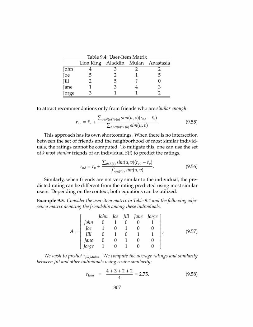
Table 9.4: User-Item MatrixLion King Aladdin Mulan Anastasia

John 4 3 2 2Joe 5 2 1 5Jill 2 5 ? 0Jane 1 3 4 3Jorge 3 1 1 2

to attract recommendations only from friends who are similar enough:

ru,i = r̄u +

∑v∈N(u)∩F(u) sim(u, v)(rv,i − r̄v)∑

v∈N(u)∩F(u) sim(u, v). (9.55)

This approach has its own shortcomings. When there is no intersectionbetween the set of friends and the neighborhood of most similar individ-uals, the ratings cannot be computed. To mitigate this, one can use the setof k most similar friends of an individual S(i) to predict the ratings,

ru,i = r̄u +

∑v∈S(u) sim(u, v)(rv,i − r̄v)∑

v∈S(u) sim(u, v). (9.56)

Similarly, when friends are not very similar to the individual, the pre-dicted rating can be different from the rating predicted using most similarusers. Depending on the context, both equations can be utilized.

Example 9.5. Consider the user-item matrix in Table 9.4 and the following adja-cency matrix denoting the friendship among these individuals.

A =

John Joe Jill Jane JorgeJohn 0 1 0 0 1Joe 1 0 1 0 0Jill 0 1 0 1 1

Jane 0 0 1 0 0Jorge 1 0 1 0 0

, (9.57)

We wish to predict rJill,Mulan. We compute the average ratings and similaritybetween Jill and other individuals using cosine similarity:

r̄John =4 + 3 + 2 + 2

4= 2.75. (9.58)

307

r̄Joe =5 + 2 + 1 + 5

4= 3.25. (9.59)

r̄Jill =2 + 5 + 0

3= 2.33. (9.60)

r̄Jane =1 + 3 + 4 + 3

4= 2.75. (9.61)

r̄Jorge =3 + 1 + 1 + 2

4= 1.75. (9.62)

The similarities are

sim(Jill, John) =2 × 4 + 5 × 3 + 0 × 2

√29√

29= 0.79. (9.63)

sim(Jill, Joe) =2 × 5 + 5 × 2 + 0 × 5

√29√

54= 0.50. (9.64)

sim(Jill, Jane) =2 × 1 + 5 × 3 + 0 × 3

√29√

19= 0.72. (9.65)

sim(Jill, Jorge) =2 × 3 + 5 × 1 + 0 × 2

√29√

14= 0.54. (9.66)

Considering a neighborhood of size 2, the most similar users to Jill are Johnand Jane:

N(Jill) = {John, Jane}. (9.67)

We also know that friends of Jill are

F(Jill) = {Joe, Jane, Jorge}. (9.68)

We can use Equation 9.55 to predict the missing rating by taking the intersec-tion of friends and neighbors:

rJill,Mulan = r̄Jill +sim(Jill, Jane)(rJane,Mulan − r̄Jane)

sim(Jill, Jane)= 2.33 + (4 − 2.75) = 3.58. (9.69)

Similarly, we can utilize Equation 9.56 to compute the missing rating. Here,we take Jill’s two most similar neighbors: Jane and Jorge.

rJill,Mulan = r̄Jill +sim(Jill, Jane)(rJane,Mulan − r̄Jane)sim(Jill, Jane) + sim(Jill, Jorge)

308

+sim(Jill, Jorge)(rJorge,Mulan − r̄Jorge)sim(Jill, Jane) + sim(Jill, Jorge)

= 2.33 +0.72(4 − 2.75) + 0.54(1 − 1.75)

0.72 + 0.54= 2.72 (9.70)

9.4 Evaluating Recommendations

When a recommendation algorithm predicts ratings for items, one mustevaluate how accurate its recommendations are. One can evaluate the (1)accuracy of predictions, (2) relevancy of recommendations, or (3) rankingsof recommendations.

9.4.1 Evaluating Accuracy of Predictions

When evaluating the accuracy of predictions, we measure how close pre-dicted ratings are to the true ratings. Similar to the evaluation of supervisedlearning, we often predict the ratings of some items with known ratings(i.e., true ratings) and compute how close the predictions are to the trueratings. One of the simplest methods, mean absolute error (MAE), com-putes the average absolute difference between the predicted ratings andtrue ratings,

MAE =

∑i j |r̂i j − ri j|

n, (9.71)

where n is the number of predicted ratings, r̂i j is the predicted rating, andri j is the true rating. Normalized mean absolute error (NMAE) normalizesMAE by dividing it by the range ratings can take,

NMAE =MAE

rmax − rmin, (9.72)

where rmax is the maximum rating items can take and rmin is the minimum.In MAE, error linearly contributes to the MAE value. We can increase thiscontribution by considering the summation of squared errors in the rootmean squared error (RMSE):

RMSE =

√1n

∑i, j

(r̂i j − ri j)2. (9.73)

309

Example 9.6. Consider the following table with both the predicted ratings andtrue ratings of five items:

Item Predicted Rating True Rating1 1 32 2 53 3 34 4 25 4 1

The MAE, NMAE, and RMSE values are

MAE =|1− 3|+ |2− 5|+ |3− 3|+ |4− 2|+ |4− 1|

5= 2. (9.74)

NMAE =MAE5− 1

= 0.5. (9.75)

RMSE =

√(1− 3)2 + (2− 5)2 + (3− 3)2 + (4− 2)2 + (4− 1)2

5. (9.76)

= 2.28.

9.4.2 Evaluating Relevancy of Recommendations

When evaluating recommendations based on relevancy, we ask users ifthey find the recommended items relevant to their interests. Given a setof recommendations to a user, the user describes each recommendationas relevant or irrelevant. Based on the selection of items for recommenda-tions and their relevancy, we can have the four types of items outlinedin Table 9.5. Given this table, we can define measures that use relevancy

Table 9.5: Partitioning of Items with Respect to Their Selection for Recom-mendation and Their Relevancy

Selected Not Selected TotalRelevant Nrs Nrn Nr

Irrelevant Nis Nin Ni

Total Ns Nn N

310

information provided by users. Precision is one such measure. It definesthe fraction of relevant items among recommended items:

P =Nrs

Ns. (9.77)

Similarly, we can use recall to evaluate a recommender algorithm, whichprovides the probability of selecting a relevant item for recommendation:

R =Nrs

Nr. (9.78)

We can also combine both precision and recall by taking their harmonicmean in the F-measure:

F =2PR

P + R. (9.79)

Example 9.7. Consider the following recommendation relevancy matrix for a setof 40 items. For this table, the precision, recall, and F-measure values are

Selected Not Selected TotalRelevant 9 15 24Irrelevant 3 13 16Total 12 28 40

P =9

12= 0.75. (9.80)

R =9

24= 0.375. (9.81)

F =2 × 0.75 × 0.375

0.75 + 0.375= 0.5. (9.82)

9.4.3 Evaluating Ranking of Recommendations

Often, we predict ratings for multiple products for a user. Based on thepredicted ratings, we can rank products based on their levels of interest-ingness to the user and then evaluate this ranking. Given the true rankingof interestingness of items, we can compare this ranking with it and reporta value. Rank correlation measures the correlation between the predictedranking and the true ranking. One such technique is the Spearman’s rank

311

correlation discussed in Chapter 8. Let xi, 1 ≤ xi ≤ n, denote the rankpredicted for item i, 1 ≤ i ≤ n. Similarly, let yi, 1 ≤ yi ≤ n, denote the truerank of item i from the user’s perspective. Spearman’s rank correlation isdefined as

ρ = 1 −6∑n

i=1(xi − yi)2

n3 − n, (9.83)

where n is the total number of items.Here, we discuss another rank correlation measure: Kendall’s tau. We

say that the pair of items (i, j) are concordant if their ranks {xi, yi} and {x j, y j}Kendall’s Tauare in order:

xi > x j, yi > y j or xi < x j, yi < y j. (9.84)

A pair of items is discordant if their corresponding ranks are not in order:

xi > x j, yi < y j or xi < x j, yi > y j. (9.85)

When xi = x j or yi = y j, the pair is neither concordant nor discordant.Let c denote the total number of concordant item pairs and d the totalnumber of discordant item pairs. Kendall’s tau computes the differencebetween the two, normalized by the total number of item pairs

(n2

):

τ =c − d(n

2

) . (9.86)

Kendall’s tau takes value in range [−1, 1]. When the ranks completelyagree, all pairs are concordant and Kendall’s tau takes value 1, and whenthe ranks completely disagree, all pairs are discordant and Kendall’s tautakes value −1.

Example 9.8. Consider a set of four items I = {i1, i2, i3, i4} for which the predictedand true rankings are as follows:

Predicted Rank True Ranki1 1 1i2 2 4i3 3 2i4 4 3

312

The pair of items and their status {concordant/discordant} are

(i1, i2) : concordant (9.87)(i1, i3) : concordant (9.88)(i1, i4) : concordant (9.89)(i2, i3) : discordant (9.90)(i2, i4) : discordant (9.91)(i3, i4) : concordant (9.92)

Thus, Kendall’s tau for the rankings is

τ =4 − 2

6= 0.33. (9.93)

313

9.5 Summary

In social media, recommendations are constantly being provided. Friendrecommendation, product recommendation, and video recommendation,among others, are all examples of recommendations taking place in socialmedia. Unlike web search, recommendation is tailored to individuals’interests and can help recommend more relevant items. Recommendationis challenging due to the cold-start problem, data sparsity, attacks on thesesystems, privacy concerns, and the need for an explanation for why itemsare being recommended.

In social media, sites often resort to classical recommendation algo-rithms to recommend items or products. These techniques can be di-vided into content-based methods and collaborative filtering techniques.In content-based methods, we use the similarity between the content (e.g.,item description) of items and user profiles to recommend items. In collab-orative filtering (CF), we use historical ratings of individuals in the form ofa user-item matrix to recommend items. CF methods can be categorizedinto memory-based and model-based techniques. In memory-based tech-niques, we use the similarity between users (user-based) or items (item-based) to predict missing ratings. In model-based techniques, we assumethat an underlying model describes how users rate items. Using matrixfactorization techniques we approximate this model to predict missingratings. Classical recommendation algorithms often predict ratings forindividuals. We discussed ways to extend these techniques to groups ofindividuals.

In social media, we can also use friendship information to give rec-ommendations. These friendships alone can help recommend (e.g., friendrecommendation), can be added as complementary information to classi-cal techniques, or can be used to constrain the recommendations providedby classical techniques.

Finally, we discussed the evaluation of recommendation techniques.Evaluation can be performed in terms of accuracy, relevancy, and rank ofrecommended items. We discussed MAE, NMAE, and RMSE as methodsthat evaluate accuracy, precision, recall, and F-measure from relevancy-based methods, and Kendall’s tau from rank-based methods.

314

9.6 Bibliographic Notes

General references for the content provided in this chapter can be found in[138, 237, 249, 5]. In social media, recommendation is utilized for variousitems, including blogs [16], news [177, 63], videos [66], and tags [257]. Forexample, YouTube video recommendation system employs co-visitationcounts to compute the similarity between videos (items). To performrecommendations, videos with high similarity to a seed set of videos arerecommended to the user. The seed set consists of the videos that userswatched on YouTube (beyond a certain threshold), as well as videos thatare explicitly favorited, “liked,” rated, or added to playlists.

Among classical techniques, more on content-based recommendationcan be found in [226], and more on collaborative filtering can be foundin [268, 246, 248]. Content-based and CF methods can be combined intohybrid methods, which are not discussed in this chapter. A survey of hybridmethods is available in [48]. More details on extending classical techniquesto groups are provided in [137].

When making recommendations using social context, we can use addi-tional information such as tags [116, 254] or trust [102, 222, 190, 180]. Forinstance, in [272], the authors discern multiple facets of trust and applymultifaceted trust in social recommendation. In another work, Tang etal. [273] exploit the evolution of both rating and trust relations for socialrecommendation. Users in the physical world are likely to ask for sugges-tions from their local friends while they also tend to seek suggestions fromusers with high global reputations (e.g., reviews by vine voice reviewersof Amazon.com). Therefore, in addition to friends, one can also use globalnetwork information for better recommendations. In [274], the authorsexploit both local and global social relations for recommendation.

When recommending people (potential friends), we can use all thesetypes of information. A comparison of different people recommendationtechniques can be found in the work of Chen et al. [52]. Methods thatextend classical techniques with social context are discussed in [181, 182,152].

315

9.7 Exercises

Classical Recommendation Algorithm

1. Discuss one difference between content-based recommendation andcollaborative filtering.

2. Compute the missing rating in this table using user-based collabora-tive filtering (CF). Use cosine similarity to find the nearest neighbors.

Le Cercle Cidade La vitaGod Rouge de Deu Rashomon e bella r̄u

Newton 3 0 3 3 2Einstein 5 4 0 2 3Gauss 1 2 4 2 0Aristotle 3 ? 1 0 2 1.5Euclid 2 2 0 1 5

Assuming that you have computed similarity values in the followingtable, calculate Aristotle’s rating by completing these four tasks:

Newton Einstein Gauss EuclidAristotle 0.76 ? 0.40 0.78

• Calculate the similarity value between Aristotle and Einstein.

• Identify Aristotle’s two nearest neighbors.

• Calculate r̄u values for everyone (Aristotle’s is given).

• Calculate Aristotle’s rating for Le Cercle Rouge.

3. In an item-based CF recommendation, describe how the recom-mender finds and recommends items to the given user.

Recommendation Using Social Context

4. Provide two examples where social context can help improve classicalrecommendation algorithms in social media.

316

5. In Equation 9.54, the term β∑n

i=1∑

j∈F(i) sim(i, j)||Ui − U j||2F is added to

model the similarity between friends’ tastes. Let T ∈ Rn×n denotethe pairwise trust matrix, in which 0 ≤ Ti j ≤ 1 denotes how muchuser i trusts user j. Using your intuition on how trustworthinessof individuals should affect recommendations received from them,modify Equation 9.54 using trust matrix T.

Evaluating Recommendation Algorithms

6. What does “high precision” mean? Why is precision alone insuffi-cient to measure performance under normal circumstances? Providean example to show that both precision and recall are important.

7. When is Kendall’s tau equal to −1? In other words, how is thepredicted ranking different from the true ranking?

317