Recognition of Cancer using Random Forests as a Bag-of...
80
Recognition of Cancer using Random Forests as a Bag-of-Words Approach for Gastroenterology Sara Isabel Moreira Francisco Supervisor: Ricardo Sousa, PhD Co-Supervisor: Miguel Coimbra, PhD Mestrado em Engenharia Biomédica June, 2015
Transcript of Recognition of Cancer using Random Forests as a Bag-of...

Recognition of Cancer using RandomForests as a Bag-of-Words Approach for
Gastroenterology
Sara Isabel Moreira Francisco
Supervisor: Ricardo Sousa, PhD
Co-Supervisor: Miguel Coimbra, PhD
Mestrado em Engenharia Biomédica
June, 2015

c© Sara Isabel Moreira Francisco: June, 2015

Faculdade de Engenharia da Universidade do Porto
Recognition of Cancer using Random Forests as aBag-of-Words Approach for Gastroenterology
Sara Isabel Moreira Francisco
Dissertation submitted to Faculdade de Engenharia da Universidade do Porto
Mestrado em Engenharia Biomédica
June, 2015


Abstract
Cancer in the gastrointestinal tract is one of the deadliest diseases worldwide. This type of cancerhas few symptoms in its early stages, thus its early diagnosis is essential to improve the survivalrate and leads to a better prognosis. Medical imaging processing technologies for cancer diagnosishave been evolving during the last century, especially endoscopes. They allow the acquisition ofimages of the tissues on the gastrointestinal tract with good resolution. Techniques to analyze theseimages have been developed and have been used by Computer Aided Diagnosis (CAD) systems.
In gastroenterology, CAD systems techniques have allowed physicians to analyze endoscopicimages using this tool as a first or second opinion, or even as an educational program. Cancerrecognition in the gastroenterology tract is a complex challenge in which only trained physicianshave a high rate of success. Some pattern recognition solutions covering this issue have alreadybeen explored in the past. However, these solutions need to be adjusted or self-tailored and areunable to automatically learn the best features to describe the data. In our approach, we extractpixel-based information (patches) and generate a Bag of Words (BoW) using Random Forests(RF) to hierarchically cluster and describe the patterns on the images.
Our experimental study is made over a dataset of chromoendoscopy images, to which we stud-ied the tuning of all the relevant parameters. Our methodology presented its optimal performancefor the following processing parameters: images converted to grayscale; patches with 5×5 pixelsare descriptive enough; the methodology performs better when using just a part of the patches,even when chosen randomly; the number of trees in the forest and the number of node per treeinfluences the performance of the methodology, providing better performance for intermediatevalues (when computational complexity is taken into account); one-versus-all strategy was used toclassify with Support Vector Machines (SVM). Finally we evaluated our proposed methodologyfrom a global point of view, obtaining 23.07± 2.83% of mean error. This is a competitive re-sult, when compared to the standard methodologies used in gastroenterology and a methodologysuitable to be used in a medical environment, with near-real time feedback to physicians.
Keywords: Gastroenterology; Computer Vision; Random Forests; Bag of Words.

ii

Resumo
O cancro no trato gastrointestinal é uma das doenças mais mortais em todo o mundo. Este tipo decancro tem poucos sintomas nos primeiros estadios da doença, aquando o diagnóstico é essencialpara maior probabilidade de sobrevivência dos pacientes. As tecnologias de diagnóstico deste can-cro evoluíram ao longo do último século, especialmente os endoscópios. Eles permitem a obtençãode imagens dos tecidos do trato gastrointestical com uma resolução e qualidades suficientes paraserem analisadas utilizado sistemas de diagnóstico assistido por computador (CAD).
Em gastroenterologia, os sistemas CAD têm tido um papel importante na avaliação de imagensde endoscopia, como ferramentas de primeira ou segunda opinião para os médicos, ou mesmocomo um programa de aprendizagem. O reconhecimento de cancro no trato gastrointestinal éum desafio complexo onde apenas os médicos especialistas são capazes de fazer um diagnósticoaltamente preciso. De forma a colmatar as lacunas existentes, algumas soluções para o reconhec-imento de padrões têm sido exploradas. No entanto, para que estas soluções sejam viáveis emgastroenterologia, é necessária a intervenção de investigadores para cada novo tipo de imagens.As metodologias existentes não são capazes de identificar e descrever automaticamente os padrõese/ou as características mais discriminativas das imagens. A solução que propomos neste trabalhovisa apresentar uma alternativa que vá ao encontro das anteriores limitações.
A nossa metodologia extrai informação diretamente dos pixeis, sob a forma de patches, geraum Bag of Words utilizando Random Forests, a partir do qual é feito um clustering hierárquico,quantificando os diferentes padrões existentes nas imagens. Esta quantificação permite criar umhistograma por cada imagem, o qual tratamos por Vocabulário. O Vocabulário é a entrada para aetapa da classificação.
Este trabalho apresenta a metodologia utilizada e o respetivo estudo experimental para umproblema multi-classe, tendo como objeto de estudo um conjunto de imagens obtidas por cromoen-doscopia. O estudo contemplou, além de uma apresentação detalhada de toda a abordagem, umaescolha dos melhores parâmetros. Após este estudo, concluímos que esta metodologia é capaz decaptar melhor a informação relevante quando as imagens são convertidas para escalas de cinzento;os patches com 5 pixels de lado extraem informação suficiente para este contexto; o desempenhoda metodologia é superior quando utilizados apenas alguns dos patches, ainda que escolhidos deforma aleatória; o número de árvores na floresta e o número de nós por árvore influenciam o de-sempenho do método, permitindo o melhor desempenho para valores intermédios (quando temosem conta o custo computacional); a estratégia one-versus-all foi utilizada garantindo robustez naclassificação de 3 classes, onde utilizamos Support Vector Machines. Finalmente, avaliamos ametodologia que propomos de um ponto de vista global, obtendo 23.07± 2.83% de erro médio,utilizando os melhores parâmetros para o dataset em questão. Este resultado é competitivo quandocomparado com as metodologias aplicadas atualmente em gastroenterologia. A metodologia é,ainda, aplicável quase em tempo real, sendo adequada para uma utilização em ambiente médico.
Keywords: Gastroenterologia; Visão por Computador; Random Forests; Bag of Words.
iii

iv

Agradecimentos
Sou uma pessoa de agradecimentos. Gosto da palavra obrigada, já que geralmente é mais fácil nãoajudar e que acho o exercício da gratidão essencial. Assim, hoje quero agradecer à informalidadedesta secção que me permite não ser científica e pelo contrário, prática e emocional, agradecendo atodos os que permitiram que eu chegasse ao fim deste percurso ainda com alguma sanidade mental(coisa que duvidei ser possível até hoje).
Antes de mais, agradeço aos orientadores deste trabalho. Ao Ricardo que me acompanhou,ainda que às vezes não compreendendo as minhas razões para encarar este trabalho como um fimem vez de um princípio. E ao Miguel, que me integrou tão bem, permitiu contactar com um mundoque não é o meu, passando nas entrelinhas uma das minhas mensagens favoritas: trabalhar comamizade e em equipa é sempre mais fácil.
Agradeço aos amigos que se mantiveram fortíssimos e presentes mesmo com todas as minhaspromessas de tempo falhadas; agradeço à Filipa, ao Francisco, aos Maneis, à Carla, à Inês, àJoana, à Sofia, ao Fernando, ao Gonçalo, ao Ivan, à Francisca, à Mariana, à Bárbara, ao Tiago, àLiliane, ao Rui, à Anabela, ao Cristiano, ao Tó, ao Diogo (Bolacha), ao Nuno (Rocky), ao Zé, àMila, à Liseta, ao Tiago Branco, ao Edgar, à Marta, à Ivana, ao outro Tiago, à Xana, ao Castro, aoLemos, à Vera e ainda a todos os que estão por perto desde há muitos anos pela energia positiva,carinho, amizade e pela festa com quilos de chocolate; tudo para conseguirem tornar estes mesesmuito mais motivadores e interessantes (e tornaram)! Obrigada também por me acompanharemnas aventuras por um mundo melhor, por partilharem o valor das experiências diferentes, dosconhecimentos transversais e por me bengalarem e relembrarem do que eu era antes disto tudo.
Aqui também tenho de agradecer aos meus pais, não só pelos chocolates, mas acima de tudopor simplesmente confiarem (exatamente como eu gosto) e por proporcionarem tudo o que fossenecessário, acreditando que chegaria facilmente ao fim.
Finalmente, sem dúvida o melhor e maior apoio emocional e incondicional, agradeço ao Pedro.Não existindo agradecimentos suficientes para ele, uma vez que a compreensão para com o meumundo de mil paixões, o amor, a paciência, a omnipresença e a confiança não têm medidas paraagradecimento.
Obrigada!
Sara Francisco
v

vi

Contents
List of Figures ix
List of Tables xi
List of Abbreviations xiii
1 Introduction 11.1 Overview . . . . . . . . . . . . . . . . . . . . . . . . . . . . . . . . . . . . . . 11.2 Motivation . . . . . . . . . . . . . . . . . . . . . . . . . . . . . . . . . . . . . . 21.3 Software . . . . . . . . . . . . . . . . . . . . . . . . . . . . . . . . . . . . . . . 21.4 Objectives . . . . . . . . . . . . . . . . . . . . . . . . . . . . . . . . . . . . . . 21.5 Contributions . . . . . . . . . . . . . . . . . . . . . . . . . . . . . . . . . . . . 31.6 Document Structure . . . . . . . . . . . . . . . . . . . . . . . . . . . . . . . . . 3
2 Cancer in the Gastrointestinal track and Technologies 52.1 Overview . . . . . . . . . . . . . . . . . . . . . . . . . . . . . . . . . . . . . . 5
2.1.1 Endoscopes . . . . . . . . . . . . . . . . . . . . . . . . . . . . . . . . . 92.2 Computer Vision in Gastroenterology . . . . . . . . . . . . . . . . . . . . . . . 14
2.2.1 Image Processing . . . . . . . . . . . . . . . . . . . . . . . . . . . . . . 152.2.2 Machine Learning . . . . . . . . . . . . . . . . . . . . . . . . . . . . . 182.2.3 Open Issues . . . . . . . . . . . . . . . . . . . . . . . . . . . . . . . . . 19
3 Random Forests for Visual Representation in Gastroenterology Examinations 213.1 Decision Trees and Random Forests . . . . . . . . . . . . . . . . . . . . . . . . 233.2 Image Acquisition and Processing . . . . . . . . . . . . . . . . . . . . . . . . . 253.3 Visual Representation . . . . . . . . . . . . . . . . . . . . . . . . . . . . . . . . 263.4 Image Recognition . . . . . . . . . . . . . . . . . . . . . . . . . . . . . . . . . 27
4 Results and Discussion 314.1 Dataset . . . . . . . . . . . . . . . . . . . . . . . . . . . . . . . . . . . . . . . 314.2 Methodology and Experimental Study . . . . . . . . . . . . . . . . . . . . . . . 32
4.2.1 Error and Statistical Significance Assessment . . . . . . . . . . . . . . . 324.2.2 Image Processing and Feature Extraction . . . . . . . . . . . . . . . . . 334.2.3 Random Forest . . . . . . . . . . . . . . . . . . . . . . . . . . . . . . . 384.2.4 Recognition of Cancer . . . . . . . . . . . . . . . . . . . . . . . . . . . 40
4.3 Best Model Assessment and Discussion . . . . . . . . . . . . . . . . . . . . . . 41
5 Conclusions and Future Work 45
vii

viii CONTENTS
A Tables of Results 47
B IJUP Abstract 53
C Summary Paper 55
Bibliography 59

List of Figures
2.1 In (a), the anatomical location of the gastrointestinal tract is shown. The typi-cal histology of tissues on the gastrointestinal tract is presented in (b). Adaptedfrom Seeley et al. [47]. . . . . . . . . . . . . . . . . . . . . . . . . . . . . . . . 6
2.2 Relevant statistics about the incidence and mortality of cancer on the gastrointesti-nal tract, and its relationship with other types of cancer. . . . . . . . . . . . . . . 7
2.3 Representative images of seven endoscopy technologies: (a) High-resolution en-doscopic image of the surface of normal mucosa. (b) HME of normal intestinalmucosa and the same image on (e), seen with NBI and HME (Haidry and Lovat[21]). (c) AFI in the normal colon (Fujiya et al. [16]). (d) Indigo carmine (thedye) chromoendoscopy of a mucosal lesion detected in a patient with Barrett’sesophagus (Haidry and Lovat [21]).(f) Mucosal capillary and surface pattern weredetected with FICE with magnification (Yoshida et al. [71]). (g) Images of normaltissue using probe based CLE ([21]). . . . . . . . . . . . . . . . . . . . . . . . . 12
2.4 Overview of the pipeline of acquisition and processing of endoscopic images bya CAD systems, focusing the image description stag, which is the main focus ofthis work. . . . . . . . . . . . . . . . . . . . . . . . . . . . . . . . . . . . . . . 14
3.1 Overview of the pipeline of our methodology to build a classifier model for gas-troenterology images. The major contributions of our work are related with theBoW and vocabulary construction. . . . . . . . . . . . . . . . . . . . . . . . . . 22
3.2 In (a), the binary tree corresponding to the partitioning of input space and in (b)an illustration of a two-dimensional input space that has been partitioned into fiveregions. Adapted from Bishop et al. [4]. . . . . . . . . . . . . . . . . . . . . . . 23
3.3 Image processing stages of the acquired endoscopy video: frames are merged intoa single view, rescaled and segmented though the physician-annotated masks. . . 25
3.4 Representation of the average-patch that pass in each node. Different patterns aredistinguishable in different nodes, suggesting a good separation of the input datainto different visual words. . . . . . . . . . . . . . . . . . . . . . . . . . . . . . 27
4.1 Images describing different types of patterns from the gastrointestinal tract thatare representative of our dataset . . . . . . . . . . . . . . . . . . . . . . . . . . 32
4.2 Average error with respect to patch width. . . . . . . . . . . . . . . . . . . . . . 354.3 Average error with respect to the number of randomly chosen patches. . . . . . . 374.4 Average error variation with respect to the number of nodes and the number of trees. 40
ix


List of Tables
2.1 Techniques used for gastrointestinal cancer detection (Yuan [72] and Lee et al. [32]). 82.2 Main achievements in Endoscopy (Berci and Forde [3]). . . . . . . . . . . . . . 92.3 Summary of the current endoscopy techniques used applications (Liedlgruber and
Uhl [34]). . . . . . . . . . . . . . . . . . . . . . . . . . . . . . . . . . . . . . . 13
4.1 Average errors for 20 runs varying the color space. . . . . . . . . . . . . . . . . 344.2 Average errors for 20 runs varying the scaling of the image between the original
size, 50% and 25%. . . . . . . . . . . . . . . . . . . . . . . . . . . . . . . . . . 354.3 Average error for 20 runs varying the size of the patch and the extraction of rotation
information. . . . . . . . . . . . . . . . . . . . . . . . . . . . . . . . . . . . . . 364.4 Average Error with respect to patch selection strategy: random selection and ap-
proximation to the centroid generating using k-means. . . . . . . . . . . . . . . . 374.5 Average error with respect to the patch normalization. . . . . . . . . . . . . . . . 384.6 Average error with respect to the vocabulary normalization. . . . . . . . . . . . . 394.7 Average errors and statistical significance values with respect to the generation of
a SVM classifier using different kernels. . . . . . . . . . . . . . . . . . . . . . . 414.8 Average confusion matrix obtained for this problem, using the optimized parame-
ters of the algorithm. Class "1" refers to the normal tissue images and the "2" andthe "3" refer to dysplasia and metaplasia images, respectively. The methodologydistinguish better the class "1" from the others than the classes "2" from the "3",suggesting that the major difficulty is in distinguish between classes with clanges. 42
4.9 Average error comparing the information extraction stage using SIFT or patch-method, as well as, comparing the BoW method using k-Means and BoW. . . . . 43
A.1 List of the tests with respective parapeters variation (continuation in Table A.2) . 48A.2 List of the tests with respective parameters variation and average error (continua-
tion in Table A.3). . . . . . . . . . . . . . . . . . . . . . . . . . . . . . . . . . . 49A.3 List of the tests with respective parameters variation and average error. . . . . . . 50A.4 List of the tests with respective parameters variation and average error (continua-
tion in Table A.5). . . . . . . . . . . . . . . . . . . . . . . . . . . . . . . . . . . 51A.5 List of the tests with respective parameters variation and average error (continua-
tion in Table A.6). . . . . . . . . . . . . . . . . . . . . . . . . . . . . . . . . . . 51A.6 List of the tests with respective parameters variation and average error. . . . . . . 51A.7 Average error varying the number of trees of the RF and number of nodes for tree
(continuation in Table A.8). . . . . . . . . . . . . . . . . . . . . . . . . . . . . . 52A.8 Average error varying the number of trees of the RF and number of nodes for tree. 52
xi


List of Abbreviations
AFI Autofluorescence ImagingAGF Autocorrelation Gabor FiltersBoW Bag of Visual WordsCAD Computer Aided DiagnosisCCD Charge Coupled DeviceCLE Confocal Laser EndomicroscopyCT Computer TomographyCV Computer VisionDOG Difference of GaussiansFICE Fujinon Intelligent ChromoendoscopyFN False NegativesFP False PositivesGLCM Gray Level Co-occurrence MatrixGLCM Gray Level Difference MatrixHME High Magnification Endoscopek-NN k-Nearest NeighborsLBP Local Binary PatternsLTP Local Ternary PatternsMRI Magnetic Resonance ImagingNBI Narrow Band ImagingRF Random ForestRGB Red, Green and BlueSIFT Scale Invariant Feature TransformSUSAN Smaller Univalue Segments Assimilating NucleusSVM Support Vector MachineTN True NegativesTP True PositivesWCE Wireless Capsule Endomicroscopy
xiii

Chapter 1
Introduction
1.1 Overview
Prevention is better than cure.
Desiderius Erasmus (1466–1536)
The prevention of all diseases is certainly the best cure, although not always possible. Cancer
is a leading cause of death worldwide, justifying the need for its prevention. It is caused by changes
in the genetic information of cells, that lead to an uncontrolled division and growth of new ones.
Cells lose their predefined function, causing the failure of tissues. In case of malignancy, it can
also affect the tissues of other organs, spreading widely through the human body1.
The difficulty of the forethought of its appearance, the lack of early symptoms and the im-
possibility of detecting symptoms from cells in the whole body in routine procedures makes the
diagnosis a difficult task, stimulating the exponential increase of research in this field. Early de-
tection and possible intervention in the human body can increase the life expectancy in cancer
patients.
Cancer in the gastrointestinal track is one of the most common types of cancer (Siegel et al.
[50]), with 1.8 million deaths per year worldwide. Technology to detect and treat cancer in its early
stage has developed greatly in the last two centuries (Berci and Forde [3]), although 30% of the
deaths still occur in the developed countries. In this group of countries, innovative technologies,
such as computer systems, made the bridge between the physician and the devices of inspection
of the gastrointestinal track, to reduce the subjectiveness of the detection, diagnosis, treatment and
monitoring of lesions.
Nowadays, thanks to the technology a physician is able to detect cancer with great accuracy,
diagnosing and distinguishing between different stages of the disease. Nevertheless, mortality rate
is still too high and the role of prevention is to decrease it. There are some existing limitations,
such as the time, the dependence of the image features and the computation complexity of process-
ing medical images, which are the bottom line of this work. Moreover, an inexperienced physician
1According to the World Health Organization’s Cancer Fact Sheet number 297, February 2011
1
2 Introduction
faces moments of doubts and a wrong diagnosis of cancer must be avoided. Here, the technology
and the existing Computer Vision (CV) techniques commonly used in Computer Aided Diagno-
sis (CAD) Systems for gastroenterology to overcome the limitations faced by the physicians are
discussed and a new methodology is proposed and characterized.
1.2 Motivation
In the past few years, CAD systems have established themselves as important tools for physicians
daily practice (e.g. in pulmonary (Wormanns et al. [69]) and breast (Jiang et al. [27]) cancer,
for the detection of tumor masses). Acting as a reliable second opinion for the diagnosis, these
systems are capable of extracting quantitative information from medical images and, thus, guide
the physician (Kuo et al. [31]).
Relevant medical fields of research, which is the case of gastroenterology have been using
these methodologies with good results. Typical diagnosis systems are based on endoscopic probes,
which capture images of the gastroenterological tract. The physician looks for specific patterns in
those images and with the help of such systems he can complement his decision about the patients’
lesion.
Current CV methodologies encompass devising hand-made features for describing natural or
biological images. The success achieved so far is limited however due to the large amount of
possible variations that an object can have in an image. In this dissertation, we explore how
a system can be designed to analyze gastroenterology images without requiring heavy human
interaction.
1.3 Software
All the tests were performed using Mathworks Matlab R2012b and the VLFEAT library 2.
1.4 Objectives
This work aims at understanding the relevance and how engineering tools can be used to detect
early on various stages of cancer in the gastrointestinal tract. We intend to explore the character-
istics of the medical instrumentation currently in use, as well as understand how adequate both
the existing and novel CV solutions for pattern recognition. The main objective of this work is to
develop a methodology that processes, describes and classifies endoscopic images with precision.
It is supposed to automatically learn the most discriminative patterns which allow to distinguish
between different stages of gastric cancer without the intervention of a researcher.
2http://www.vlfeat.org

1.5 Contributions 3
1.5 Contributions
The contributions of this work are listed below:
1. A new methodology using Random Forests (RF) for the recognition of different stages of
cancer (normal tissue, dysplasia and metaplasia) in gastroenterology images, improving the
accuracy rate exhibited in previous work in the field.
2. The proposed methodology software, available online in http://sarafranciscothesis.pt.vu/;
1.6 Document Structure
This document is organized as follows. In Chapter 2, we start by contextualizing this research,
emphasizing its biomedical relevance while giving insight about the physiology of the gastroin-
testinal system and existing instrumentation for endoscopy; finally, we describe the current CV
methodologies used to analyze endoscopy images. In Chapter 3, we fully describe our proposal
for endoscopic images analysis and classification methodology. Finally, in Chapter 4 and in 5
the results of the evaluated parameters are discussed and the conclusions of out work presented,
respectively.


Chapter 2
Cancer in the Gastrointestinal trackand Technologies
Cancer on the gastrointestinal tract is one of the most severe cancers, due to its high mortality
rate and prevalence. Its detection, similarly to what happens with the other types of cancer, is no
longer a strictly medical task. Indeed, it combines the medical know-how with relevant advances
in oncology and novel and innovative techniques for an objective characterization of tissues, the
latter provided and developed by biomedical engineers.
The relationship between medicine and engineering has become closer over the past few years,
allowing the physicians to evolve from simple semiology (analysis of naked-eye signs and symp-
toms) to the usage of tools which provide an objective and reliable evaluation of the patient, (for
example, endoscopes or, more recently, computer-aided diagnosis systems). These solutions, al-
though innovative, are still not versatile enough to be able to address unknown or unseen variations
of the morphology of tumors, as well as the eyes of experienced physicians can. This handicap
is also extended to inexperienced physicians, motivating the development of a gastroenterology
image analysis system that embeds cancer recognition strategies, allowing a future training or
examination to have a reliable evaluation of new and challenging cases.
In this Chapter the context of our work is presented, providing a transversal understanding of
the whole gastroenterological cancer detection problem. We start by exploring the characteristics
of the cancer of the gastrointestinal tract, the importance of its study, followed by the instrumen-
tation technology for cancer detection. Finally, the methodology proposed in this work, as well
as the CV methodologies used for gastroenterology images analysis in which it is based on are
introduced.
2.1 Overview
Gastrointestinal cancer occurs in the organs of the digestive system, which includes the esophagus,
stomach, gallbladder, liver, pancreas, stomach, small intestine, colon and rectum. Each of these
organs has a unique shape and is composed of a type of tissue exposed to different conditions,
5

6 Cancer in the Gastrointestinal track and Technologies
making the cancer detection procedures difficulty and requiring them to be individually adapted
(Seeley et al. [47]). Nevertheless, all cancers can be caused by eating habits, derive from other
pathologies or some hereditary conditions. There are five stages of the disease (grades from 0 to
IV), enforcing the need for early treatments (Jankowski and Hawk [25]).
In this section, the importance of cancer detection, the physiology of the organs on the gas-
trointestinal tract, the limitations of the available detection devices and technology will be studied.
The main goal is to draw conclusions about the current detection and diagnosis technology and
the research fields in which improvements are required.
Morphology and Physiology
Figure 2.1a depicts the gastrointestinal tract, emphasizing the organs of the digestive system
relevant for this work, since these organs allow an acquisition of images. These organs have a
similar histology, although playing distinct roles in the digestive process. There are four main
cellular layers: the inner mucosa, the submucosa, the muscular layer and the external serosa,
Figure 2.1b (Seeley et al. [47]).
(a) The gastric canal. (b) Histology of the gastroenterologic tract.
Figure 2.1: In (a), the anatomical location of the gastrointestinal tract is shown. The typicalhistology of tissues on the gastrointestinal tract is presented in (b). Adapted from Seeley et al.[47].
There are three main types of cancer in the gastrointestinal tract: metaplasia, dysplasia and
neoplasia (Kapadia [28]). The first one consists simply in the differentiation from a healthy cell to
its abnormal or mutated version. On the other hand, dysplasia, although still a reversible process,
promotes a disordered growth and maturation of tissues. Neoplasia is an irreversible change of
cells. The grade associated to a certain cancer depends on the location of the tumor and its specific
histology. The stage 0 of the gastrointestinal cancers is called dysplasia. The tumor invades or is
generated in the mucosa of an organ. The following stages require the spreading through the inner
layers of a tissue. The most severe stage (IV) happens when the tumor spreads systemically and

2.1 Overview 7
metastasis are found in other organs (Jankowski and Hawk [25]).
Statistics and Mortality
Currently, more than 14 million people per year are victims of cancer worldwide. 2,1 million
of them present pathologies on the colorectum, esophagus or stomach (see Figure 2.2a). There are
around 1,8 million deaths every year, 30% in the more developed countries, where more advanced
technology and diagnostic procedures are used (Ferlay et al. [13]).
Gast. Tract Resp. System Liver Breast Prostate0
0.5
1
1.5
2
2.5IncidenceMortality
Type of cancerNum
bero
fCas
es(m
illio
nsof
pers
ons)
(a) Cancer incidence and death rates in 2014, by typeof cancer.
I II III IV0102030405060
ColonRectumStomach
Cancer Stage
Surv
ival
Rat
e(%
)
(b) Survival rate by type of cancer on stomach, rectumand colon.
Distant Region Localized010203040506070
Cancer Location
Surv
ival
Rat
e(%
)
(c) Survival rate with respect to location of esophaguscancer.
Figure 2.2: Relevant statistics about the incidence and mortality of cancer on the gastrointestinaltract, and its relationship with other types of cancer.
Figure 2.2b and Figure 2.2c present the survival rates of cancer of the gastrointestinal tract1.
1Adapted from: http://www.cancer.org/index

8 Cancer in the Gastrointestinal track and Technologies
As can be observed, the survival rate increases with the early cancer detection (Areia et al. [2]).
The analysis of images in the gastrointestinal tract allows the visualization of structures and plays
a major role in the early detection of the pathology. From this, and based on the aforementioned
statistics, it is mandatory to improve the cancer detection procedures and the existing technology.
Diagnosis and Detection
The common techniques used to diagnose gastrointestinal cancer are briefly present in Ta-
ble 2.1. Cancer detection has a complex nature and may involve different medical routines, from
general exams to high-resolution medical imaging procedures.
Table 2.1: Techniques used for gastrointestinal cancer detection (Yuan [72] and Lee et al. [32]).
General exam of the body Performed by a general practitioner, in which systemicsigns of the disease are searched for. The patient historyand its health habits are discussed and evaluated. Patientswith problems on the structures of the gastrointestinal tractare directed to a gastroenterologist.
X-Ray The most common and non-invasive medical imaging rou-tine. In it the organs are observed. From a two view acqui-sition, it is possible to infer if abnormal masses are presentin the abdominal cavity. However, X-ray is not enough foran early detection.
Endoscopy An endoscope passes down the throat of the patient. Endo-scopes are thin, flexible, camera-holding and illuminatedtubes. They allow the observation of the esophagus, stom-ach and the first section of the small intestine. Potentialabnormal areas are searched for and biopsies (tissue sam-ples) can be collected for further laboratory analysis. Thereis a myriad of endoscope configurations possible. It is themost used technique to diagnose cancer on the gastroin-testinal tract.
Virtual Endoscopy Magnetic Resonance Imaging (MRI) and Computer To-mography (CT): High-resolution medical imaging tech-niques, only used when the other diagnostic proceduresfail. They can provide with high certainty the location ofthe abnormal masses and are usually essential to direct thetreatment based on the location of the tumor. Provide rele-vant information for surgical procedures.
The early detection of the disease demands the observation and histological examination of the
abnormal cells. Therefore, the endoscopy is nowadays the most used procedure for these cases.
In its early years, 1860s, endoscopy found two physical limitations: the gastrointestinal tract
is not straight and there is no light inside the body (Sivak [54]). Some years after the invention of
the light bulb, a mirror and light system was developed, eliminating the problem of the darkness.

2.1 Overview 9
However, only in the 1960s was the flexibility of the device achieved. It was then possible to use
an eye piece and optic fiber, strategically organized to transmit not just light, but also to acquire
images. This is the true ancestor of the device used nowadays, the flexible endoscope. Modern
endoscopes are very compact devices, including a Charge Coupled Device (CCD) for acquiring
images or film and a light source on the distal tip (see Table 2.2). Endoscopes are also equipped
with an accessory channel, allowing the entrance of medical instruments to collect tissue samples
in a minimal invasive procedure (Berci and Forde [3] and Liedlgruber and Uhl [34]).
Table 2.2: Main achievements in Endoscopy (Berci and Forde [3]).
Year Achievement
1868 First Gastroscopy, credited to Kaussmaul1961 First device with articulated lenses and prisms1920 Flexible quartz fibers first concept1954 First flexible endoscope model1969 Invention of CCD
Clinical literature states that the usage of endoscopes provides high early detection rates and
leads to a good prognosis, thus preventing the cancer from evolving into more dangerous stages.
Since medical endoscopy is a minimally invasive and relatively painless procedure, allowing us
to inspect the inner cavities of the human body, endoscopes play an important role in modern
medicine. However, an accurate cancer detection and diagnosis is still difficult. This is mostly due
to the lack of visual cues that suggest the presence of cancer in its early stages (Singh et al. [52]).
Complementing endoscopy with biopsy allowed physicians to collect direct histological in-
formation from the organ being analyzed (Yuan [72]) and the technological advancements in en-
doscopy digital tools improved the cancer recognition rate, when compared to ancestor techniques
(Lee et al. [32]).
Both the design of endoscopes and the ability to take digital pictures motivated the usage of
CAD support systems for gastrointestinal images. These are intended to help the diagnosis, act-
ing as a first or complementary opinion to physicians in general applications. Specifically on the
gastroenterology domain, the implementation of common CV tools has made it possible to detect
and describe quantitatively the visual features leading to an useful automated decision (Liedlgru-
ber and Uhl [34]). Such could be achieved using MRI or CT-scans but, although reliable, such
diagnostic methods are computationally complex, costly and require users to be highly familiar
with technology (Liedlgruber and Uhl [34]). This created the need for a simple, practical and af-
fordable tool, developed for a user-shaped evaluation of gastrointestinal images, capable of being
implemented on a daily routine practice.
2.1.1 Endoscopes
An endoscope is a medical device capable of acquiring both images and even tissue samples from
the gastrointestinal tract. Although a lot of configurations are possible, all endoscopes share some

10 Cancer in the Gastrointestinal track and Technologies
characteristics: (a) they are composed of a flexible tube; (b) illumination and image acquisition
tools are incorporated; (c) this device has an accessory channel where some claws can be added,
especially for biopsy samples capture. Different endoscopy techniques are described below.
Standard and High Definition Endoscope: The standard definition endoscope is equipped with
a CCD chip, acquiring an image signal with 100-400 pixels and images with a defined aspect ratio
of 4:3. The High-definition endoscope has a similar configuration but provides images of higher
resolutions. Consequently, the physician can detect subtle changes in the mucosa more easily. Its
images have a resolution 10 times higher, two different images aspect ratio and its monitors can
display progressive images while in progress. The frame rate of 60 times per second decreases
the amount of noise and allows the accurate capture of fast motions (Subramanian and Ragunath
[60]). See Figure 2.3a.
High Magnification Endoscope (HME): The technological advances have lead to the devel-
opment of the HME. It has electronically movable lenses which allow real time visualization of
mucosa morphology in greater detail (Singh et al. [53]). The endoscopic image is zoomed up to
150-fold, while keeping high detail and resolution. This is a major improvement when compared
to common digital zoom or electronic magnification systems. In HME, the image is moved closer
to the display, decreasing the number of observable and the image resolution. Most conventional
endoscopes are capable of electronic magnification of 1.5-fold to 2-fold but require a compatible
processor.
These endoscopes were widely studied by Stevens et al. [59], in a work that looked at the early
diagnosis of cancer in the gastrointestinal tract, especially metaplasia and dysplasia. Although
this technique is easily available with high resolution, it was designed to increase the visualization
quality and lacks a diagnose-oriented framework. See Figure 2.3b.
Autofluorescence Imaging (AFI): Recent endoscopes use autofluorescence imaging (AFI). AFI
detects the natural fluorescence of tissues, which is emitted by specific light-excitable molecules.
It is possible to capture color differences in the fluorescence emission in real time, because of
their unique fluorescence spectra. This technique allows tissue characterization and can be used
to detect a significant number of patients with high grade early cancer (Singh et al. [53]). See
Figure 2.3c.
Chromoendoscope: This technique is based on the enhancement of the surface of the mucosa
by applying different dyes. Depending on the followed protocol, different stains are used, thus
making different anatomical structures more prone to be observed. Obviously, there are endo-
scopes with different sensibility for each dye (Rácz and Tóth [43]). There are two essential stages
in chromoendoscopy: (1) removal of mucous, normally using water; and (2) dye application. A
more detailed overview on this technique is available on (Singh et al. [53]). See Figure 2.3d.

2.1 Overview 11
Virtual Chromoendoscopes: Virtual Chromoendoscopy is nowadays the most widely used tech-
nique in endoscopy. Being a reliable alternative to the time-consuming chemical chromoen-
doscopy, it allows the enhancement of the mucosal surface without applying color dyes. A better
contrast of the vascular patterns on the mucosa is often achieved recurring to Computer Vision
techniques.
• Narrow Band Imaging (NBI): The need for a simpler endoscopy technique led to the
development of the NBI, firstly described in Ohyama et al. [39]. The common endoscopes
illuminate the scene of interest using white light, which results from the fusion of three light
waves: green, blue and red. NBI narrows the bandwidths of blue (440-460 nm) and green
(540-560 nm) wave light, while the contribution of the red wave light is totally discarded
from the emitted light (Singh et al. [53]). The main advantage of narrowing the green and
blue light spectra is an enhancement of the microvasculature pattern (due to a superficial
penetration of the mucosa and to an absorption peak of hemoglobin for these wavelengths).
Images obtained using NBI endoscopes were tested with promising results in Curvers et al.
[10], Mannath et al. [36]. See Figure 2.3e.
• i-scan: This technique consists of three types of algorithms: Surface Enhancement, Con-
trast Enhancement and Tone Enhancement. Surface Enhancement enhances the light-dark
contrast on the image, by obtaining the luminance intensity data for each pixel. Then, al-
gorithms for the detailed observation of the mucosal surface structure are applied. Contrast
Enhancement digitally adds blue color in relatively dark areas: the luminance intensity data
for each pixel is obtained and subtle irregularities around the surface are computationally
enhanced. Both enhancement functions work in real time without impairing the original
color of the organ. Additionally, both are suitable for screening endoscopy to detect gas-
trointestinal tumors at an early stage. Finally, Tone Enhancement dissects and analyzes the
individual RGB components of a normal image. Then, the color spectrum of each compo-
nent is altered and recombined with the other components into a single, new color image.
This approach was designed to enhance mucosal structures and subtle changes in color. The
i-scan technology leads us to easier detection, diagnosis and treatment of gastrointestinal
diseases (Kodashima and Fujishiro [30]).
• Fujinon Intelligent Chromoendoscopy (FICE): FICE can simulate an infinite number of
wavelengths in real time. The system has 10 channels that are designed to explore the entire
mucosal surface. Each channel corresponds to the three specific RGB wavelength filters,
but there is no setting specifically used for a given gastroduodenal condition (Coriat et al.
[7]). See Figure 2.3f.
Confocal Laser Endomicroscopy (CLE): CLE provides high-resolution microscopic images
at sub cellular resolution, streaming the deepest layers of the gastrointestinal mucosa. The term
confocal refers to the alignment of both the illumination and collection systems in the same focal

12 Cancer in the Gastrointestinal track and Technologies
(a) High Definition Endo-scope image
(b) High MagnificationEndoscope image
(c) Autofluorescence im-age
(d) Chromoendoscopy im-age
(e) NBI and High Defini-tion Endoscope image
(f) Fujinon IntelligentChromoendoscopy Image
(g) CLE image
Figure 2.3: Representative images of seven endoscopy technologies: (a) High-resolution endo-scopic image of the surface of normal mucosa. (b) HME of normal intestinal mucosa and thesame image on (e), seen with NBI and HME (Haidry and Lovat [21]). (c) AFI in the normal colon(Fujiya et al. [16]). (d) Indigo carmine (the dye) chromoendoscopy of a mucosal lesion detectedin a patient with Barrett’s esophagus (Haidry and Lovat [21]).(f) Mucosal capillary and surfacepattern were detected with FICE with magnification (Yoshida et al. [71]). (g) Images of normaltissue using probe based CLE ([21]).
plane. Laser light is focused through a pinhole at the selected depth via the same lens (Liedlgruber
and Uhl [34]). See Figure 2.3g.
Unfortunately, the visual criteria for malignancy is still under clinical evaluation, as stated
in Shui-Yi Tung et al. [49], thus making it impossible for the scientific community to evaluate the
potential of this new technique. Additionally, such a complex methodology requires experienced
users to correctly manipulate it and thus achieve good results.

2.1 Overview 13
Wireless Capsule Endomicroscopy (WCE): The inspection of the small intestine is a difficult
task due to its long and convoluted shape. WCE was designed to overcome this limitation and to
make endoscopic procedures safer, less invasive, and more comfortable for the patient.
In this case, the endoscope is not a flexible tube but a capsule that the patient swallows. The
small capsule is equipped with a light source, lens, camera, radio transmitter, and batteries. Pro-
pelled by peristalsis, the capsule travels through the digestive system for about eight hours and
automatically takes more than 50 000 images. These are transmitted via wireless to a recorder
worn outside the body (Liedlgruber and Uhl [34]). Currently, WCE seeks not only to inspect the
small intestine, but other organs such as the colon or the esophagus. The main drawbacks of WCE
consist in the lack of ability to obtain biopsy samples, contrary to other endoscopy techniques.
Table 2.3 presents a summary of the main applications of the technologies previously described
and currently commercialized (Subramanian and Ragunath [60]). Although recent solutions are
accurate and equipped with recent technology, thus the best solution adapted for each case that
implies a combination of more than one technique, the perfect endoscope is still to be developed.
(Song and Wilson [56]).
Table 2.3: Summary of the current endoscopy techniques used applications (Liedlgruber and Uhl[34]).
Endoscope Application Target Tissue
Standard and HD Used combined with other technolo-gies like die-based and Virtual Chro-moendoscopy
Surface enhancement.Reduce Artifacts.
High Magnification Identification of neoplasia Surface/vascular detail.
AFI Identification or early detection of neo-plasia
Displasia
NBI Identification of neoplasia speciallycombined with Magnification En-doscopy.
Vascular Contrast of cap-illaries and submucosaenhancement
I-scan and FICE Identification of neoplasia speciallycombined with Magnification En-doscopy.
Structural and vascularenhancement
CLE Identification of neoplasia Subcelular structures
Conclusion: The endoscopic devices presented previously allow the physicians to inspect all
the inner cavities of the alimentary canal, even the intestine, thanks to the capsule endoscopy.
Although the differences in the resolution of the images acquired by different devices, the differ-

14 Cancer in the Gastrointestinal track and Technologies
ences between the acquired images by these devices are not the main limitation for the accuracy
of current CV techniques. The major constraint is in the existent methodologies which are still
not able to extract the most descriptive features or describe better the information contained in the
medical images. This constraints and the attempts to overcome this in the gastroenterology field
are presented in the next Section.
2.2 Computer Vision in Gastroenterology
The acquisition of images of the gastroenterological tract using endoscopic probes is a procedure
prone to noise. As it is performed in non-controlled conditions, some problems regarding illu-
mination, rotation, shadows or occlusion occur. CV in gastroenterology has to deal with these
vicissitudes and also with very feeble visual patterns which hampers the lesion recognition capa-
bility.
The previously developed works in this field of research comprised a wide variety of standard
CV techniques. Nevertheless, they are still limited in some of the aforementioned acquisition
constraints or the resultant classifier is just optimized to a range of images, instead of being robust
to any dataset. In this field it would be valuable the use of an algorithm able to robustly extract the
relevant features, thus allowing its application in any gastroenterology images.
Although we are trying to answer to a medical problem, it is also a pattern recognition chal-
lenge. A possible solution may include other image processing algorithms that have not been tried
before in this field.
Figure 2.4 shows a common pipeline for the acquisition and processing of endoscopic images
in a CAD system. This document has previously presented endoscopic image acquisition devices
and in this section we detail the procedure for the processing and recognition of cancer in gastroen-
terology endoscopic imaging. In particular, we give special emphasis to the Feature Extraction and
Image Description in order to introduce our proposal, since they are the most challenging stages
and the scientific community looks forward to guarantee better accuracies. After, we introduce the
strengths and limitations of the state of the art methodologies, as well as a methodology designed
by us to overcome such weaknesses, proposed in Section 3.
Figure 2.4: Overview of the pipeline of acquisition and processing of endoscopic images by aCAD systems, focusing the image description stag, which is the main focus of this work.

2.2 Computer Vision in Gastroenterology 15
2.2.1 Image Processing
Feature analysis intends to gather information from images. A feature is a point or image region
that is salient, relevant and distinctive from its neighbors (Zitova and Flusser [73]). The ideal type
of features must be invariant to noise, which can be caused by undesired motion of endoscopic
probes, shadows or occlusions. A good feature presents at least the following characteristics:
• Repeatability: which is achieved when different images of the same gastrointestinal lesion
show corresponding feature points;
• Distinctiveness: obtained when a certain feature is specific for a certain lesion;
• Accuracy: features must be located exactly where distinct points of the lesion are found
(Tuytelaars and Mikolajczyk [65]).
This canonical definition was firstly applied to static scenes or objects, relying on the detec-
tion of corners (as Harris in Harris and Stephens [23] or Smallest Univalue Segment Assimilating
Nucleus (SUSAN) corner detectors in Smith and Brady [55]), edges or high-level features. These
latter ones are already associated to image description and representation. In the gastroenterology
field, high-level features have been used in studies with different purposes: detection of gastric
ulcers (Kodama et al. [29]), to make a generic description of the intensity values and detect inten-
sities changes along different regions of the images (Häfner et al. [20]) and differentiate between
cell-types in colorectal polyps (Gross et al. [18]). They present some pleasing results for standard
scenes, but not flexible and accurate enough to deal with the acquisition problems and to guar-
antee the extracted features are relevant enough for a powerful description. Due to this, standard
methods, such as corner and edge detectors, have been discarded since and are absent from recent
works in this field.
Along with simple detectors and high-level feature extraction methodologies, other approaches
were developed. Region detectors, which often enhance homogeneous regions in images, were
one of those. A region is an image area that has an averaging intensity distinct from that of the
surrounding neighbors, defined by applying custom-made segmentation algorithms. These regions
are expected to be descriptive of the image content and class that is being searched for. Although
important, this is not the focus of this thesis, since we aim at describing the regions of interest
in gastroenterology images, not detecting such regions. In fact, our dataset consists in previously
segmented images by experienced physicians.
Frequency Domain Features
Frequency Domain features are a decomposition of the image information of the spatial do-
main into frequency domain, obtained by Fourier transformations. In the Fourier domain, each
point represents a particular frequency contained in the spatial domain image. From the new spec-
trum of features that Fourier transformations gives, it is possible to describe the image from a
different perspective (Liedlgruber and Uhl [34]). In Haefner et al. [19], the authors explore the

16 Cancer in the Gastrointestinal track and Technologies
application of Fourier filters to distinguish between six types of mucosal texture and pit-patterns,
each one with specific spatial distribution and response to the filters. Fourier transformations were
also used by Vécsei et al. [67], applying its highly discriminative power to the classification of
duodenal images. The authors mapped the images on the Fourier Space using a bank of filters
and selected the most discriminative features for each RGB color channel using an Evolutionary
Algorithm. As a whole, Fourier transformations can be used to obtain the power spectrum of an
image, compute statistical features and use them for classification, as described by Liedlgruber
and Uhl [34].
Wavelets also allow the mapping of images into the frequency domain. They are described
as a mathematical tool, useful to extract specific information from images by the parametrization
and customization of the wavelet. Its analysis provides information similar to what occurs in the
human visual system, performing a hierarchical edge detection at multiple levels of resolution
(Liedlgruber and Uhl [34]).
From the different types of wavelets that can be applied to image processing methods, Gabor
Filters take the lead in the gastroenterology field (Riaz et al. [44]). Autocorrelation Gabor filters
(AGF) were firstly presented by Gabor [17]. They are based in the principles of a simple cell in
the mammalian visual cortex. These cells are characterized by their band pass nature and direction
selectivity, making them respond only to specific spatial frequencies and orientations. The filtering
stage guarantees their invariance to illumination, rotation, scale and translation. This is because,
although the image can be rotated or translated, the frequency content of the image remains the
same, thus making them always detectable (Riaz et al. [44]). According to Riaz et al. [44], AGF
is capable of performing a feature detection stage together with the computation of image descrip-
tors, while being invariant to rotation and illumination changes. Then these descriptors are used
by a previously trained classifier to obtain a suggestion of the diagnosis.
Although new approaches, such as the one presented in this thesis, explore the application of
other machine learning methodologies to the analysis of gastroenterology images, frequency do-
main features remain a strong research field in this topic, since they mimic the sensing capabilities
of the human visual system. It is believed that following this premise, we can be able to extract
more and better information about the patterns in an image.
Spatial Domain Features
Spatial Domain Features consider texture and pixel-based information, by building histograms
and computing statistical parameters from the extracted data. In fact, the standard methodologies
for the classification of gastroenterology images often rely on texture analysis techniques (Liedl-
gruber and Uhl [34]) and correlate changes with the intensity with their location in the images.
One of the most well known methodologies for texture analysis is the LBP (Local Binary
Patterns)(Ojala et al. [40]). This methodology searches for uniform patterns computed over an
image, whose occurrence is counted into an histogram, effectively estimating the distribution of
microstructures (edges, lines, regions). The detection of these structural features allows to describe

2.2 Computer Vision in Gastroenterology 17
the images. This quantization of feature distribution can be performed by combining multiple
operator for multiresolution analysis: different search radius and angles. This analysis is centered
on the image intensities inside a small processing window (often (3x3)), that are binary labeled (0
or 1) with respect to the average intensity inside the neighborhood in which they are contained.
This processing enhances the aforementioned structures, believed to provide a good detection of
pattern changes between different images or image regions.
LBP is popular in texture analysis because of its rotation invariance. Also, the intensity dif-
ferences are not affected by minor changes in the mean luminance of images, since the intensity
values are not highly compromised. In other words, the binary pattern of the region only changes
if the gray-scale intensity of, at least, one pixel becomes higher or lower than the mean intensity in
that neighborhood. So, if no relevant changes in the gray-scale values are found, the region keeps
being defined by the same binary pattern.
An improvement was described by Tan and Triggs [61] where the LTP (Local Ternary Patterns)
were presented. This descriptor, in opposition to LBP (which describes a texture using a binary
pattern, 0 or 1), calculates the texture of a Region of Interest computing a pattern of three values.
Using ternary patterns instead of binary patterns increases the resolution of the descriptor. More
recently, in Hegenbart et al. [24], authors have started by presenting a wide study about the state of
the art methodologies for duodenal lesion classification using computer vision techniques. They
show that an affine-invariant version of the LTP can be used for the description of duodenal images
with good results. However, this methodologies are not immune to luminance and scale variations,
which interfere in the intensity value on the image.
GLCM (Gray Level Co-occurrence Matrix) is another typically used methodology in gastroen-
terology (Dhanalakshmi et al. [11]). Proposed by Haralick et al. [22], it is a matrix that counts all
the transitions between the intensities of an image region, in a specified direction and radius. Each
specific texture is defined by a set of transitions with associated probabilities, where measures such
as the contrast, energy, homogeneity, and entropy can be obtained. Although similar images allow
us to obtain similar GLCM, it is also true that completely different patterns with similar intensities
can lead to GLCM that are alike (Haralick et al. [22]).
In the subsequent years, some modifications to GLCM were introduced. One of them is
GLDM (Global Level Differences Matrix), which computes differences between the pixels on
the region of interest rather than counting intensity transitions. In Onji et al. [41] the capability of
these texture descriptors, especially to describe endoscopy images is studied. As these methods are
highly dependent on the pixel intensities, the output can be compromised by luminance changes
over time. In other words, as the endoscopic image acquisition is performed in a non-controlled
environment, the texture analysis will answer to every intensity variation, even if it is artificial or
caused by other artifacts. Thus, GLCM or GLDM may not provide the most robust solution.
In the same work, the authors show that the SIFT (Scale Invariant Feature Transform) de-
scriptor performs a better quantitative description than the GLDM for the same dataset. The SIFT
(Lowe [35]) descriptor extracts keypoints based on image texture. A SIFT keypoint is a blob-like,

18 Cancer in the Gastrointestinal track and Technologies
circular image region with a specific orientation. It is described by the following geometric pa-
rameters: the keypoint center coordinates, its scale (the radius of the region), and its orientation
(an angle)2.
Then, taking into account the selected keypoints, SIFT computes a 128-feature space descrip-
tor, invariant to translation, rotation and scale, also minimally influenced by noise and illumination.
To achieve this, SIFT searches for keypoints at various scales and positions, following the basic
strategy of the DoG (Difference of Gaussians) method (Crowley and Parker [8]). The main advan-
tage of SIFT is that, not only allows a robust localization of relevant features, but also computes
descriptive information.
Embedding Local Features in Global Image Description
The canonical separation between global and local feature extraction strategies is related to
choosing whether we want to describe image properties as a whole (global features) or to extract
relevant information from each of the sub-regions of the images (local features). Local features
provide an intuitively better description, since they are not affected by noise in distant regions
of the images, are less prone to lose fine changes in the texture of images and distinguish better
between foreground and background (Tuytelaars and Mikolajczyk [65]). Their better descriptive
power is also due to their distinctive representation of relevant regions of the image, while remain-
ing invariant to viewpoints and illumination changes (Trzcinski et al. [64]).
However, powerful local descriptions require a very subtle tuning of parameters, otherwise the
extracted information lacks context and we miss important information about the images. More-
over, Tuytelaars and Mikolajczyk [65] state that, unlike what it is expected, global descriptors work
well for images with distinctive colors and at least, with homogeneous or characteristic texture. In
gastroenterology images, texture homogeneity is almost impossible to achieve, thus making global
descriptors a weak option, despite the obvious need for context. Although the image description
using local features and global features may seem unlikely to achieve, their fusion into a single
powerful description strategy would overcome these individual weaknesses and provide a more
reliable tool for feature extraction.
Following Chatfield et al. [6], this study explores the potentialities of visual bagging. Briefly,
we intend to extract local features to improve the discriminative power and overcome possible
acquisition constraints, then combining it into a Bag of Visual Words, that globally describes the
image using the local extracted features. This mapping contextualizes the extracted information
and is expected to guarantee a more fine and detailed characterization.
2.2.2 Machine Learning
In the gastroenterology field, the vast majority of studies have been using SVM (Support Vector
Machines) (Vapnik and Vapnik [66]) and k-NN for classification (k-Nearest Neighbors), due to its
importance and versatility in pattern recognition [34]. Although the competitive accuracy rates and
2http://www.vlfeat.org/api/sift.html

2.2 Computer Vision in Gastroenterology 19
computational simplicity of k-NN, a supervised classification method that labels an instance based
on the closest samples on the feature space, SVM is the state-of-the-art classification method.
Details about SVM methodology can be found in Chapter 3.
Among the most common usages of SVM in this field of research are precise tumor detection
(Li and Meng [33]) and colorectal polyps classification (Tischendorf et al. [63]). Conversely, k-
NN has been applied in a prominent recent work, to find abnormalities in the inner cavities of the
gastrointestinal system (Nawarathna et al. [38]).
2.2.3 Open Issues
The methods presented in the previous sections are the most commonly used solutions in gas-
troenterology. However, in this thesis, we propose an alternative solution for the problem in
hands, based on recent works in different computer vision applications. They have given some
insight into how to solve the problems related to the classification of cluttered images, with oc-
cluded regions of interest and the typical rotation, multiresolution and illumination variations. The
proposed solutions, that quantify the number of times each different pattern (visual word) occurs
in the images (vocabulary), are expected to be translated to the evaluation gastroenterology im-
ages. The set of visual words is know, in CV, as Bag of Words (BoW). More details about BoW
generation can be found in the next chapter.
As BoW requires randomness for a representative description, the first strategies were designed
using k-means (Csurka et al. [9]), since the centroid locations are randomly defined at the start of
each repetition of the algorithm. However, these locations are not linked to the input data, dimin-
ishing the correlation of the Bag of Words to the true characteristics of the images. To overcome
this, a RF-based framework was proposed by Shotton et al. [48]. The proposed method guides
the creation of randomized classification trees using the information on the input images, each
node of each tree being a splitting instance that tries to separate, even slightly, different patterns.
This way, image regions with varying information are grouped separately, while maintaining the
required randomness (Yao et al. [70]), and allowing the computation of quantitative information
via histograms. Those histograms can provide distinctive information between images with dif-
ferent classes (more detailed information in Chapter 3). The method proposed by Shotton et al.
[48], along with the preliminary study presented by Moosmann et al. [37], although presenting
good performances, lack data ranking, i.e. they only use the leaf nodes of each tree on the RF
and assume that the branching capabilities of a decision capture all the differences between the
patterns on the leaf nodes. However, small changes can provide relevant information that is not
included in the analysis when only the terminal nodes are considered. We look forward to evaluate
the importance of the information on the splitting nodes, along with that on the terminal ones.
A preliminary attempt to characterize gastroenterology images using BoW has been proposed
by Sousa et al. [58], which implements a BoW generation stage using K-means after image de-
scription using dense SIFT. The obtained results were promising and motivate the usage of RF to
generate a more reliable BoW of the data.

20 Cancer in the Gastrointestinal track and Technologies
These achievements can provide solutions to overcome the limitations on the classification of
endoscopic images using CAD systems. It is expected that a robust BoW can be created from
extracting the most discriminative local information on sub-regions of the images and combining
them into a single global descriptor. By doing this, we overcome the lack of resolution of a
global description, by centering the analysis into specific regions that enclose highly discriminative
feature points. Low-level patterns and variations, i.e. more detailed information, is obtained, with
the plus that noisy data is likely to be discarded. This way, only relevant information is kept and
used for classification.

Chapter 3
Random Forests for VisualRepresentation in GastroenterologyExaminations
In this Chapter we present the main contribution of this thesis, describing a new methodology for
cancer recognition in gastroenterology images. The majority of CAD systems rely on machine
learning techniques that fit a classification model to features extracted from the images being
analyzed. It is common that features are not powerful enough to distinguish between different
classes. Even images descriptors computed after the extraction of these features lack on the ca-
pacity of identifying the most discriminative patterns. To overcome this, several methods have
been proposed. One efficient way of handling this pattern recognition challenge is to define visual
words (textons) and quantify its frequency on the input data. In CV, the ensemble of visual words
is called BoW.
Considering a text categorization challenge, the occurrences of each word can be counted to
build a global histogram, summarizing the document content in respect to each word frequency
(Moosmann et al. [37]). This parallelism explains the usability and the potential of this method
for our work. We survey and list all the patterns on an image into a visual codebook and count
the amount of times that each pattern appears on the image being classified. Such counting pro-
cedure can be perceived as a histogram of occurrences in which image content is summarized and
described with simplicity, thus making the construction of an effective classifier easier. This ap-
proach has been used to describe common scenes and detect well-defined objects by Shotton et al.
[48] with promissory results.
We use RF to generate this BoW, which is a novelty in gastroenterology images classification.
RF carry descriptive power and establish an hierarchy over the input data, separating it into patterns
in a way that is expected to capture the richness and the diversity of patterns in an image.
The RF is generated by constructing decision trees, which allow the ranking of the data throw
the criterion defined by each node of the trees. In each of the nodes of a tree the separation of the
different patterns is expected. Although building the decision tree as a classifier, because of its na-
21

22 Random Forests for Visual Representation in Gastroenterology Examinations
ture, this scheme gives relevant information for pattern recognition, since it is possible to describe
the images throw this information. In order to increase the strength of this approach we generate
an ensemble of trees, here called forest. Furthermore, each tree is generated independently with
randomized attribute choices and threshold definitions, meaning that RF allow a hierarchical clus-
tering that occurs in an unique way in each tree, but always anchored to the intrinsic nature of the
input data.
This approach is embedded in a larger processing pipeline, shown in Figure 3.1, which aims
at analyzing and classifying endoscopic images dealing with the aforementioned acquisition con-
straints. Our approach automatically renders representative features from the images, dismissing
the need for a specialist to guide its extraction.
The method presented here is an advance in the classification of gastroenterology images be-
cause it can accurately distinguish between different classes without requiring previous knowledge
about features. In our specific application we are dealing with a multiclass problem, in which the
differences between the classes are not evident and we expect to require a robust and highly de-
scriptive method to extract relevant information from the images.
Figure 3.1: Overview of the pipeline of our methodology to build a classifier model for gastroen-terology images. The major contributions of our work are related with the BoW and vocabularyconstruction.
The methodology presented herein comprises the following stages: (a) image acquisition; (b)image processing for denoising purposes; (c) feature extraction stage, in which the images are
sampled into patches - arrays with intensities of the pixels of a certain region; (d) generation of
a Bag of Words from the extracted image information, using Random Forests; (e) building the
Vocabulary using the generated words to describe all the images; (f) train a SVM classifier using
the descriptive information from the Vocabulary to predict the class of new images.
In the following Sections we start by providing a theoretical contextualization about Decision
Trees and RF and then describe the processing stages of our algorithm, including Vocabulary
generation and classification.

3.1 Decision Trees and Random Forests 23
3.1 Decision Trees and Random Forests
Decision trees are statistical approaches designed for decision support strategies, because they are
self-explanatory, handle both numeric and nominal input attributes and deal well with possible
errors or missing values on the dataset ( Rokach [46]). They take the input data and subject it to a
sequence of binary decisions. This sequence can be seen as an iterative creation of a tree, which
branches left or right at each node, or decision point. In other words, the input data follows a
specific path while it descends the tree and until it reaches a leaf node, as shown in Figure 3.2a.
(a) Binary tree. (b) Two-dimensional input space divided.
Figure 3.2: In (a), the binary tree corresponding to the partitioning of input space and in (b) anillustration of a two-dimensional input space that has been partitioned into five regions. Adaptedfrom Bishop et al. [4].
Decision Tree Growth: Let us consider the feature space, whose whole representation can be
seen as the top node of the tree. The structure of a Decision Tree corresponds to the nodes and
branches contained in it or, in other words, how the feature space is divided. New nodes are added
by starting at the root node and applying a split criterion to decide whether the tree branches left or
right. This split criterion is decided by taking into account the most representative feature (the one
that leads to the minimal expected error of classification) of the input data and comparing it with
a splitting variable, by exhaustive search. The splitting criterion can take into account different
statistical moments of the input data (as mean, variance or others). After this first branching, we get
two child-nodes, each one containing a part of the input data. Further divisions of the feature space
occur at each node, with the corresponding input data being branched similarly to what happens
in the first node. Both the most representative feature for branching, xn and splitting variable at
each node, θn, are depicted in Figure 3.2a. Trees are grown until the expected classification error
remains constant or becomes lower than a pre-specified threshold.
Pruning: Bishop et al. [4] state that the none of the available splits produces a significant re-
duction in error, and yet after several more splits a substantial error reduction is found. For this
reason, it is common to grow larger trees, using a stopping criterion based on the number of data

24 Random Forests for Visual Representation in Gastroenterology Examinations
points associated with the leaf nodes, and then prune back the resulting tree. Pruning the tree
corresponds to defining the resulting depth of the tree, that is expected to be large enough to allow
enough descriptive splittings, but remain as small as possible to avoid redundant branches or over-
splitting of the data. More detailed information about the pruning criteria can be found in Bishop
et al. [4].
Classification and Clustering: For any new sample to be classified, we determine the subregion
in which it falls the most. We start at the top node of the tree and follow a path to the final depth,
branching down according to the splitting variables ( Bishop et al. [4]). The final predicted label is
the most voted terminal region and, for the majority of the applications, this is the only thing that
matters. However, the potentialities of decision trees are not restricted to classification, since they
naturally cluster the data when splitting. This carries descriptive power about the input data. Such
a description can be measured by counting the number of times each subregion is reached by the
instances of the data when descending a tree. This inspired the search for tree-based approaches
that take advantage of this clustering to generate codebooks of the input data, in machine learning,
known as BoW.
Random Forests: Using a single Decision Tree is not a guarantee itself that the different patterns
of the data are correctly learned. It has been described that the tree structure is very sensitive to
small changes in the dataset, generating variable sets of splits ( Friedman et al. [15]). Additionally,
the splits on the feature space are parallel to its axes (see Figure 3.2b) which may be suboptimal. It
is possible that the most robust split criterion for a specific input data is an oblique threshold, which
is not guaranteed by Ordinal Decision Trees, where the splitting criterion is always a constant value
on the feature space. We can overcome these drawbacks by using a set of randomly generated
Decision Trees, known as RF.
A RF is an ensemble of T decision trees. Associated with each node n in the tree is a learned
class distribution P(c|n). The whole forest contributes for the final classification by averaging the
class distributions over the terminal nodes nodes L = (l1, . . . , lT ) reached for all T trees:
P(c|L) = 1T
T
∑t=1
P(c|lt) (3.1)
RF add randomization to the learning process since each one of the trees is independently
generated and assumes a unique set of splitting criteria and branches. This way, the same input
data is differently branched and all the relevant splittings are expected to occur. Considering that
we cannot guarantee that a single Decision Tree is capable to learn the best classification model
without undesired variance and bias (caused by an erroneous parameter tuning), using RF increases
the probability of learning the underlying model that discriminates between different classes.
In this work we follow the research of Shotton et al. [48], applying RF to perform the hier-
archical clustering of local image patches into a BoW that summarizes the pattern content of the
input images. In other words, RF can be perceived as simple spatial partitions that assign a dis-

3.2 Image Acquisition and Processing 25
tinct visual word from the BoW to each leaf (Shotton et al. [48]). This hierarchical clustering is
obtained by the successive branches of the input data according to the different splitting criteria:
at the first splits we can distinguish heterogeneous patterns of the input data; while approximating
the leaf node we increasingly separate more homogeneous patterns, achieving highest levels of
descriptiveness.
K-means: K-means is commonly used for clustering the input data by defining random centroids
and assigning each instance to a class that corresponds to the closest centroid. The classification is
iteratively updated depending on the existing data until the centroids do not change. This is espe-
cially useful when we do not have labeled data, making K-means a fair solution for unsupervised
learning. Sometimes the best clustering is not possible when the random, and data-independent,
initialization of centroids is too different from the real centroids, not converging into an acceptable
solution. In this specific application, we are dealing with a dataset previously labeled by special-
ists. This means that we can explore the hierarchical clustering capabilities of RF to cluster the
data with fastness and more stability in the differentiation of different patterns, when compared to
K-means (Shotton et al. [48]), since intermediate patterns are considering into the analysis.
3.2 Image Acquisition and Processing
The output of an endoscopy is a video of the structures of the alimentary canal. It is processed by
physicians who extract at least one relevant frame, which may have undesired image artifacts. We
try to smooth such artifacts by rescaling the images. Then, physicians use custom-made software1
to define the regions of clinical interest of each image, whose masks were provided and used for
segmentation. Here, our methodology can process images with intensities described using four
different color space types: RGB, Opponent Space, CIE-LAB and Grayscale. Then, we apply a
Gaussian smoothing filter for denoising purposes. These pre-processing steps are represented in
the Figure 3.3.
Figure 3.3: Image processing stages of the acquired endoscopy video: frames are merged into asingle view, rescaled and segmented though the physician-annotated masks.
1Developed at IT - Institute of Telecommunications, Porto.

26 Random Forests for Visual Representation in Gastroenterology Examinations
Following this, we perform a feature extraction stage. As previously mentioned, features
are intended to be unique, accurate and distinctive. Our methodology aims at combining such
characteristics into a single feature extraction strategy. Nevertheless, in order to achieve this goal
some challenges arise.
Gastrointestinal images present tissues with different patterns whether they are healthy or not.
Although these patterns are easily identified by a trained physician, the task is much more compli-
cated for other professionals and, especially, computers. This is because common pattern recog-
nition strategies are designed for generic scenes or objects and are not optimized for medical
imaging. In this specific application, the quality of the pattern identification can be compromised
by acquisition constraints. Therefore, our methodology must be invariant to rotation, luminance
and scale and combining spatial information around each pixel with the intensity values to increase
the distinctiveness and reliability of the extracted features.
Our approach divides the segmented image into intensity patches of size nxn, extracted from
the annotated region into an array. Since local features have been described to be more robust to
spatial variations (Vogel and Schiele [68]) and medical conditions are often recognized by varying
patterns, our methodology looks for regional changes on patterns, thus reducing the influence of
non-related regions of the image.
Patches can be overlapped or not, depending on the user-defined patch window and spacing
between adjacent patches. If the spacing between the patches is lower than the patch size, there
are overlapping and consecutive patches share some intensities. Some overlapping may be desired
to diminish the spatial variance inside proximal regions. Tissues associated to the same class that
are spatially close are expected to have similar texture. By allowing the overlap of patches, we
guarantee that similar tissues have more similar patches.
The intensities of each patch are extracted and reshaped into a vector array. This approach
is inspired on the strategy presented by Simonyan et al. [51]. However, instead of extracting a
circular region, we look for all pixel intensities. This provides additional spatial information to the
description of a region pattern.
From here, the feature vector, containing the stored patch information is normalized to guaran-
tee independence from the original intensity range of the image. As a whole, we are anticipating
the need to search for, not only, texture information, but also context information. The feature
vector is used to initialize RF to generate BoW in the Vocabulary generation stage.
3.3 Visual Representation
RF contain all the possible patterns or visual words —textons— and in the context of our problem,
they can be seen as a BoW. If new data is given to the trees in the forest, it splits according to the
existence of similar patterns in the visual codebook.
Let us consider a patch that is given to the first tree of the RF. This patch descends the tree,
splitting its information left or right, which causes it to cross certain nodes of the tree until it
reaches a leaf node. We repeat this in all of the trees and all of the patches extracted from each

3.4 Image Recognition 27
Figure 3.4: Representation of the average-patch that pass in each node. Different patterns aredistinguishable in different nodes, suggesting a good separation of the input data into differentvisual words.
image, counting the number of times each node belongs to a descending path, generating the
Vocabulary of the images. Each patch is expected to have different terminal nodes in different
trees due to the randomness associated to their generation. However, patches which belong to
different images of the same class are expected to cross similar paths along the trees in a forest.
This is depicted in Figure 3.4.
The inspection of the RF is provided by the information organized within each tree: (a) an
array with the index of the feature vector that corresponds to the most descriptive intensity for each
patch at a specific level; (b) a split array, indicating the value for comparison with the intensity
identified in (a), allowing to decide the growth direction of the tree; (c) a two-column matrix, the
treemap, which indicates the next daughter-node in the tree, describing left and right branches.
As a whole, this inspection of the generated RF allows the collection of a set of relevant
information which describes the images. We count the number of times each node belongs to the
descending path of the patches. This counting vector behaves like a histogram of the visual words
and will be the input to build the classifier.
3.4 Image Recognition
We propose the use of SVM for the creation of a classification model, by supervised learning, tak-
ing as inputs the training data descriptor and the real class labels. The work that mostly inspired
our methodology (Shotton et al. [48]), used RF, not only for hierarchical clustering, but also for
classification. However, RF may not be optimized for the classification of medical images: they
perform well in static scenes since they take advantage for the distinct features of an objects, not
easily confused when we are dealing with common objects (their Vocabulary is highly different).
With medical images, this is not true: since all the patterns on the region of interest belong to hu-

28 Random Forests for Visual Representation in Gastroenterology Examinations
man tissue, the differences we are looking at are smooth, not very distinct and we cannot guarantee
an accurate distinction using a voting strategy on the terminal nodes (as classification RF do).
SVM were introduced by Vapnik and Vapnik [66] as a tool that fits a binary classification
model to the training data, by defining an hyperplane in the feature space that best separates the
features of different classes. Additionally, such hyperplane is expected to correctly fit the test data
thus dividing it into the two considered classes. From then, SVM have been extensively used in
machine learning applications, for image and signal classification.
We are given l training examples {xi,yi}, i = 1,... , l , where each example has d inputs xi ∈ℜd ,
and a class label with one of two values yi ∈ {−1,1}. Now, all hyperplanes in ℜd are parametrized
by a vector w, and a constant b, expressed as follows:
w · x+b = 0 (3.2)
Being w the vector orthogonal to the hyperplane. Given such hyperplane (w,b) that separates
the data, this gives the function
f (x) = sign(w · x+b) (3.3)
The hyperplane that best separates the input data into classes can be found by maximizing
its distance to the closest data points. The functional distance of each hyperplane is ≥ 1. Each
coordinate pair can define each given hyperplane (w,b), but each has a different functional distance
to a given data point (Boswell [5]). Therefore, the distance d from the hyperplane candidate to a
specific point must be normalized by the magnitude of w, as follows:
d((w,b),xi) =yi(xi ·w+b)‖w‖ ≥ 1
‖w‖ (3.4)
It is intuitive that finding the maximum distance can be achieved by minimizing ‖w‖. The
most commonly used strategy is the usage of Lagrange Multipliers, as described in Vapnik and
Vapnik [66]. The more samples we use, the better this stage is. Additionally, the bias parameter,
b can be determined taking any positive and negative support vector, x+ and x− respectively, as
follows:
b =−12(w · x++w · x−) (3.5)
The proven principle of SVM is that the input data can be perfectly separable. However,
in some cases, such separation can only be achieved if the information is mapped into higher
dimensions, thus increasing greatly the computational cost. There must be a compromise between
the fitting of the best hyperplane and a huge complexity, against a lighter processing stage and the
existence of some misclassified samples.
In fact, in real situations, a perfect separation between classes is not always possible. SVM
can be tuned using different parameters to achieve the maximum fitting. For this purpose, kernels,
power formulas that allow the mapping for higher dimensions, have been designed. Another ex-

3.4 Image Recognition 29
ample of tuned parameters is the cost, C, whose value defines the acceptable number of wrongly
classified observations during the model fitting. As concluded before: (i) SVM maximize the
distance between the hyperplane and the closest points; (ii) we often deal with misclassified ob-
servations when defining the margin, especially when the optimal separation between the data is
not feasible with low computational cost. Following this, we must define a soft-margin, one that
performs and acceptable separation of the data, while allowing some misclassifications to occur.
The growth of the margin is critical and controlled by C, the cost of each misclassified sample.
In our specific application, SVM should inspect the Vocabulary and fit the classification model
that differentiates the classes of the images. The tuning of SVM parameters will be performed
by k-fold cross-validation, to optimize the relation between the regularization parameter and the
homogeneous parameter of the kernel. Additionally, an intersection kernel is used to build the
model, since the feature vector can be interpreted as a histogram.
Multiclass classification As SVM provide a binary answer to classification problems: an ob-
servation either belongs to a specific class or not. In a multi-class problem, such as this one,
it is impossible to label all the observations in a single instance. Thus, a multiclass classifica-
tion strategy must be followed. We have chosen a one-versus-all (OVA) strategy: we compute the
probability of a certain observation to belong or not to each of the classes against the others (Sousa
et al. [57]) and then the predicted class of an observation is the one with the best score.
Other approaches would be possible, such as the method proposed by Frank and Hall [14].
This approach takes into account a linear relationship between the existing classes, which is not
completely true in gastroenterology since the evolution of patterns between different stages of
cancer is not linear. Additionally, this solution does not consider that each class is independent
from the others, and provides less comparisons than OVA.


Chapter 4
Results and Discussion
In the current Chapter we evaluate the performance of the methodology proposed in Chapter 3,
presenting and discussing the results of the experimental study performed. Here, we discuss how
the different parameters of each of the stages of our method influences the classification of new
instances, or images. In each test, we varied specific parameters, maintaining a standard parameter
configuration for the following variables:
• Images were resized to half of their original size and converted to grayscale.
• 100 patches of 5 pixels width, randomly chosen.
• Random Forests with 10 trees, each tree with 100 nodes.
• Intersection kernel and one-versus-all strategy for SVM classification.
All the tests were performed in a AMD Phenom II X4 955 CPu @ 3.20 Ghz, 8GB RAM
(64-bit) computer.
4.1 Dataset
Our dataset consists of 176 chromoendoscopic images, pre-segmentated into clinically relevant
regions according to manual annotations by an expert physician. This dataset is encompassed by
56 normal tissues and 96 metaplasia and 24 dysplasia cases (see Dinis-Ribeiro et al. [12] for more
information). A sample of our dataset is depicted in Figure 4.1. The three images presented there
are representative of the aforementioned classes.
It is possible to see different constraints to the analysis of the images in this dataset that must
be addressed in this work. The acquired images may be blurred and present specular highlights or
fluids. Moreover, there are limitations related with the acquisition procedure: the varying distance
between the probe and the tissues, possible rotation of the probe and images with regions without
clinical interest.
31

32 Results and Discussion
(a) Normal tissue. (b) Tissue with dysplasia. (c) Tissue with metaplasia.
Figure 4.1: Images describing different types of patterns from the gastrointestinal tract that arerepresentative of our dataset
4.2 Methodology and Experimental Study
The dataset presented in previous section will be the object of our study, being randomly divided
into train and test images, 30 and 146, respectively, for each test performed. We ensure that
each class is similarly represented in the training set in order to allow a similar learning of all the
classes. Moreover, we expect similar results for different dataset of gastroenterology images, since
the acquisition constraints are similar.
4.2.1 Error and Statistical Significance Assessment
The experiments assessed in the Chapter were evaluated and compared according to the following
methodologies.
Performance evaluation: Performance was assessed calculating the error according to:
Error =1c·
c
∑i=1
FNi
FNi +T Pi(4.1)
where c is the total number of classes, FN the false negative results and TP the true positives.
Tests were repeated 20 times and the mean error considered.
Statistical Significance: Statistical significance of the results was performed. The different ex-
periments were evaluated statistically in order to find if the difference between the tests is signifi-
cant or even different or similar.
The normality of the data was ensured by Jarque-Bera tests (Jarque and Bera [26] and Thade-
wald and Büning [62]) and significance was computed using two-tailed t-tests. We took p< 0.05
as criterion for significance.

4.2 Methodology and Experimental Study 33
4.2.2 Image Processing and Feature Extraction
The images were processed and some tests were assessed. Regarding the image processing, we
tuned (a) the influence of color information and (b) the influence of resizing the image before ex-
tracting the patches. Tuning the parameters regarding the extraction of information of the images
we aim at (a) the patch dimensions, (b) the influence of extracting and including rotation informa-
tion in the analysis, (c) how to select the more descriptive regions where to extract the patches, (d)the amount of valuable information to use for the subsequent stages of processing; and (e) which
is the best strategy to normalize the data extracted directly from the images.
Color: A color performance study was performed for four color spaces: grayscale, RGB, Oppo-
nent Space and CIELab. Our original images are RGB and the conversions are presented below,
considering that R, G and B stand, respectively, for the red, green and blue color channels of the
image.
As presented in Riaz et al. [45], grayscale images have performed well in gastroenterology
field. This can be explained by the existent CV methods which aim at mimic the primary visual
cortex, working mainly for detection of shapes by the existent contrast of black and white. We
converted RGB images to grayscale according to the following adopted formula (Akenine-Möller
et al. [1]):
I = 0.3×R+0.59×G+0.11×B (4.2)
However RGB color space is the most frequent, other spaces were proposed in order to mimic
the operation of the human vision system. The opponent color space is an example of this, relying
on opponent hues: yellow or blue and red or green. The human vision is not able to detect the
opponent colors at the same time and the opponent color space take advantage, transforming RGB
in three different channels: Yellow-Blue (YB), Red-Green (RG) and a monochromatic channel (I).
Starting from here, effective color features were derived and a basic representation can be obtained
by follow(Plataniotis and Venetsanopoulos [42]) :
I1 =R+G+B
3(4.3)
I2 = R−B (4.4)
I3 =2G−R−B
2(4.5)
Methods like the ones presented above perform well in specific applications but not under any
circumstances. This create the need for color spaces invariant to operation conditions. In response
to that, CIELab, which is also an opponent color space, present 3 color dimensions, L, approxi-
mating the human perception o lightness, a∗ and b∗ that correspond to RG and YB, respectively.

34 Results and Discussion
The transformation from RGB to CIELab was performed using the Mathworks Matlab built-in
rgb2lab function.
The results of the experiments performed are presented in 4.1.
Table 4.1: Average errors for 20 runs varying the color space.
Image Scale Average Error p-Value with respect toGrayscale RGB OS - standard OS - CIELab
Grayscale 23.79(±3.73)% - 0.0001 0.0001 0.0001RGB 35.33(±4.71)% - - 0.0044 0.8309
OS - standard 39.57(±4.70)% - - - 0.0335OS - CIELab 35.73(±6.71)% - - - -
Image Filtering : We filtered the images by an isotropic Gaussian kernel, with different sigmas
calculated as follows:
σ =
√(8k
)2
−0.25 (4.6)
where k corresponds to the kernel size.
The value of the sigma varies according to the kernel size; for each kernel we save a patch.
This ensures invariance to the illumination.
Image Resizing: We tested the influence of resizing the images of our dataset to 25% and 50%
of its original size (518 x 481).
The acquired images have noise and artifacts, which we intend to remove or, at least, reduce
during the pre-processing stage. One of the strategies to achieve it is resizing the images. As
presented in Table 4.2, when we resize the images to half of its original size, we have a lower
error when compared to the full-sized image. However, the means are statistically similar. This
suggests that resizing the images to 50% of its size does not compromise the content of the image
for classification and reduces the noise, taking into account that the average error decreases. On
the other hand, when classifying images resized to a quarter of its original size, we get an error
of the same range (slightly higher), however with statistically different means, suggesting that this
scale of resizing is harmful: although the image artifacts are smoothed and the computational cost
decreases, the relevant information contained in the images also becomes lost, thus compromising
the classification.
Feature Extraction: In this stage we aim at extracting relevant information from images, invari-
ant to acquisition constraints. This can be achieved by optimizing the feature extraction parameters
to guarantee maximum descriptiveness. The following settings and variables were tested:
• Patches size: 5, 11, 15, 21 and 25;
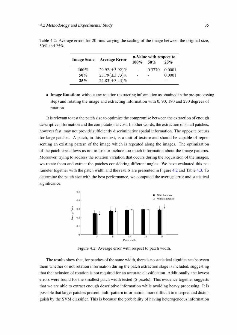
4.2 Methodology and Experimental Study 35
Table 4.2: Average errors for 20 runs varying the scaling of the image between the original size,50% and 25%.
Image Scale Average Error p-Value with respect to100% 50% 25%
100% 29.92(±3.92)% - 0.3770 0.000150% 23.79(±3.73)% - - 0.000125% 24.83(±3.43)% - - -
• Image Rotation: without any rotation (extracting information as obtained in the pre-processing
step) and rotating the image and extracting information with 0, 90, 180 and 270 degrees of
rotation.
It is relevant to test the patch size to optimize the compromise between the extraction of enough
descriptive information and the computational cost. In other words, the extraction of small patches,
however fast, may not provide sufficiently discriminative spatial information. The opposite occurs
for large patches. A patch, in this context, is a unit of texture and should be capable of repre-
senting an existing pattern of the image which is repeated along the images. The optimization
of the patch size allows us not to lose or include too much information about the image patterns.
Moreover, trying to address the rotation variation that occurs during the acquisition of the images,
we rotate them and extract the patches considering different angles. We have evaluated this pa-
rameter together with the patch width and the results are presented in Figure 4.2 and Table 4.3. To
determine the patch size with the best performance, we computed the average error and statistical
significance.
5 11 15 21 250
0.1
0.2
0.3
0.4
0.5With RotationWithout rotation
Patch width
Ave
rage
Err
or
Figure 4.2: Average error with respect to patch width.
The results show that, for patches of the same width, there is no statistical significance between
them whether or not rotation information during the patch extraction stage is included, suggesting
that the inclusion of rotation is not required for an accurate classification. Additionally, the lowest
errors were found for the smallest patch width tested (5-pixels). This evidence together suggests
that we are able to extract enough descriptive information while avoiding heavy processing. It is
possible that larger patches present multi-pattern information, more difficult to interpret and distin-
guish by the SVM classifier. This is because the probability of having heterogeneous information

36 Results and Discussion
Table 4.3: Average error for 20 runs varying the size of the patch and the extraction of rotationinformation.
Patch Width With Rotation Without Rotation p-Value
5 24.81(±4.00)% 23.79(±3.73)% 0.420711 27.84(±4.85)% 27.30(±3.86)% 0.705215 28.67(±3.87)% 29.02(±4.66)% 0.805421 29.52(±4.70)% 28.95(±3.16)% 0.665725 29.01(±4.59)% 31.20(±4.39)% 0.1406
along patches decreases. It would be interesting to study the performance of the methodology for
a patch width smaller than 5 pixels.
Patch selection: We also evaluated the preponderance that the number of patches has on the
classification task. The literature states that using the most descriptive patches leads to better
results than when we use all of the information contained on the images (Simonyan et al. [51]). To
test this hypothesis, two different experiments we prepared: (a) data randomly chosen; (b) usage
of a metric that finds the most homogeneous and the most heterogeneous patches using k-means.
The results for the randomly chosen patches are shown in Figure 4.3. Different quantities
of patches were extracted. Since the region of interest among images is variable, the number of
patches extracted per image varied between 198 and 5538. Analyzing the results, we can perceive
that, as expected, the error is higher when too few patches are selected. Furthermore, the average
error stabilizes when we reach 200 patches (when not existent, we extract the maximum patches
of an image). This means that a larger quantity of data does not, in itself, mean better and more
descriptive information. This is highly correlated with the results obtained for the inclusion or
non inclusion of rotation information: the fact that we include more information about rotation
is not expected to improve the performance of the descriptor if the information is not discrimina-
tive enough. In fact, it is not: we are simply looking at the same pattern from different angles.
The focus must be on distinguishing between different patterns, rather than assuming that includ-
ing rotated information can accurately simulate a rotation of the acquisition endoscope. More
information will diminish the discriminative capacity of Random Forests, since we have a finite
number of nodes. There is no evidence that all the different patterns can be separated, since more
data requires more splits (whose number is limited by the number of nodes we have).
The literature predicts that the performance of the classifier is expected to be higher for more
descriptive patches, than for all of the extracted information (Simonyan et al. [51]). Following
this, and considering that the behavior of the random choice of patches was promising, we tried a
methodology for the extraction of both the most homogeneous and the most heterogeneous patches
of each image. They are expected to capture, respectively, the global characteristics of the image
and small and discriminative variations on patterns between classes.
We started by choosing the patches using the k-means algorithm. Let us consider a cluster of
patches: those nearer to the cluster centroid are the most homogeneous; conversely, the farther

4.2 Methodology and Experimental Study 37
0 100 200 300 400 500 600 700 800 900 1,0000
0.2
0.4
0.6
0.8
1
Number of patches
Ave
rage
Err
or
Figure 4.3: Average error with respect to the number of randomly chosen patches.
ones are the most heterogeneous. Although we followed a correct premise, this metric presented
some flaws, since the centroids are generated randomly and we cannot guarantee that centroid is
representative enough of the homogeneity of the data. We are looking forward to understand how
to define the most reliable centroid for clustering and, from there, choose the patches. These flaws
cause the metric to perform worse, as expected, and shown in Table 4.4.
Table 4.4: Average Error with respect to patch selection strategy: random selection and approxi-mation to the centroid generating using k-means.
Patch Selection Strategy Average Error
Random Selection 23.79(±3.73)%k-Means 47.56(±5.92)%p-Value 0.0001
Patch Normalization: The basic principle of normalization is to map variables that were mea-
sured in different scales into the same range, to make a coherent comparison between them possi-
ble. Here, we are not dealing with a scale problem. Normalization aims at stabilizing the histogram
of the patches, since the pre-processing stages cause them to be saturated in some ranges.
Firstly, we process the patch intensities as follows:
pt (i) = 255− emp−(i)
mp·log255 (4.7)
where p is a row vector of the pixel intensities previously extracted and mp is the maximum value
inside the patch. After, a new transformation is applied:
pn(i) =pt (i)√
∑Nn=1 pt (i)
2 +2−52(4.8)
where N is the total number of intensities extracted. After these processing stages, L2 or z-score
normalization were tested. The results depicted in Table 4.5 show that normalization is able to
improve the performance of our method.
38 Results and Discussion
Table 4.5: Average error with respect to the patch normalization.
p-Value with respect to Average ErrorNo Normalization L2 z-score
No Normalization - 0.0001 0.0001 38.45(±5.01)%L2-Normalization - - 0.0001 23.79(±3.73)%
z-score Normalization - - 50.04(±3.87)%
4.2.3 Random Forest
The BoW was constructed using the Mathworks Matlab R2012b built-in TreeBagger function.
This function creates an ensemble of decision trees, which we previously named RF (see Sec-
tion 3.1).
We adapted the function parameters according to the problem at hand:
• We chose Deviance as Split Criterion. While building the trees, the function guarantees the
maximum deviance reduction. In other words, it weighs misclassified observations badly
optimizing the relevance of each instance.
• Pruning: was not done. Instead of using the optimal sequence found by pruning the tree
using TreeBagger 1, we grew all the trees until the pre-defined number of nodes was reached.
Our approach extends the use of RF presented by Moosmann et al. [37] and Shotton et al.
[48]. While these authors only use the information on the leaf nodes, we take advantage from the
hierarchical clustering capabilities of the trees, taking into account all the nodes on each tree. The
TreeBagger function of Matlab outputs unbalanced trees (terminal nodes can be found at any depth
and are not grown). Because of this, trees have different configurations and the same node number
occurs at different positions. To guarantee that the same node number is attributed to the same
position on the tree, we balanced the branches of the trees, introducing new child-nodes in the
pruned branches and updating the node number of the already existent ones. This guaranteed that
all of the trees had the same structure. The average error obtained using only the terminal nodes
of balanced trees to generate BoW was 25.44± 5.03%, while an average error of 23.79± 3.73%
was obtained using all of the nodes in the trees. This result suggest that the hierarchical clustering
is an advantage and using non-terminal nodes provides relevant information that is not captured
using only the leaf nodes.
As mentioned before, the randomness of the BoW generation does not always guarantees the
best descriptive power of the vocabulary. Different parameters can be varied when looking for an
adequate vocabulary while keeping the computational efficiency low:
• RF dimensions: 1-10, 50, 100, 200,300 and 500 trees;
• Number of nodes: 10, 50, 100, 200, 300, 400, 500, 800 and 1000 nodes.
1Mathworks guide for Supervised Learning.

4.2 Methodology and Experimental Study 39
The vocabulary dimensions results from the product of the aforementioned variables. The size
of our vocabulary depends both on the number of trees of the forest and the number of nodes on
each tree, as explained in Section 3. It influences the computational cost and the accuracy of our
methodology, making it necessary to find the best compromise. To address that, we varied both
the number of trees and the number of nodes, and the results are shown in Figure 4.4.
The number of nodes determines where the trees stop growing. As previously mentioned, few
nodes do not allow the Random Forests to correctly differentiate between the different patterns
in the images. Otherwise, for bigger trees, we get redundant data for the final nodes of each
tree, providing invaluable data while increasing the computational cost. Regarding the number of
trees, as they increase, the strength of the classifier improves since different ways of separating
the patterns of the input images are implemented. As always, we must find the ideal number of
nodes and the ideal number of trees, so that we can build a robust classifier while reducing the
computational cost as much as we can.
Figure 4.4 shows the variation of the average error with the number of nodes of the trees and
the size of the RF. It is visible that small trees and forests lead to a poor performance as expected,
with increased error and standard deviation. Stabilization of the results occurs for at least 50 trees
and 300 nodes. In these conditions, not only does the error but also the standard deviation reach
their minimum value.
These results are intuitive because of the reasons mentioned above: too many nodes make the
vocabulary redundant and the forest size should allow the robustness of the classifier without com-
promising the computational cost; additionally, without enough information for the description of
images, descriptive power is not ensured. Furthermore, the stabilization values for the number of
trees and the number of nodes proves our premisses: we need to increase the number of nodes to a
limit for which the information becomes redundant (leading to the stabilization of the average er-
ror), and to have the minimum number of trees that guarantees enough randomness to distinguish
patterns that the simple splitting of nodes cannot.
Vocabulary Normalization: To normalize the vocabulary we have followed the same strategy
adopted to normalize the patch intensities. The results are presented in Table 4.6.
Table 4.6: Average error with respect to the vocabulary normalization.
p-Value with respect to Average ErrorNo Normalization L2 z-score
No Normalization - 0.0130 0.0978 23.79(±3.73)%L2-Normalization - - 0.5747 26.89(±3.61)%
z-score Normalization - - - 26.12(±4.70)%

40 Results and Discussion
0 200 400 600 800 1,0000
0.2
0.4
Number of Nodes
Ave
rage
Err
or
500 Trees
0 200 400 600 800 1,0000
0.2
0.4
Number of Nodes
Ave
rage
Err
or
300 Trees
0 200 400 600 800 1,0000
0.2
0.4
Number of Nodes
Ave
rage
Err
or
200 Trees
0 200 400 600 800 1,0000
0.2
0.4
Number of Nodes
Ave
rage
Err
or
100 Trees
0 200 400 600 800 1,0000
0.2
0.4
Number of Nodes
Ave
rage
Err
or
50 Trees
0 200 400 600 800 1,0000
0.2
0.4
Number of Nodes
Ave
rage
Err
or
10 Trees
0 200 400 600 800 1,0000
0.2
0.4
Number of Nodes
Ave
rage
Err
or
9 Trees
0 200 400 600 800 1,0000
0.2
0.4
Number of Nodes
Ave
rage
Err
or
8 Trees
0 200 400 600 800 1,0000
0.2
0.4
Number of Nodes
Ave
rage
Err
or
7 Trees
0 200 400 600 800 1,0000
0.2
0.4
Number of Nodes
Ave
rage
Err
or
6 Trees
0 200 400 600 800 1,0000
0.2
0.4
Number of Nodes
Ave
rage
Err
or
5 Trees
0 200 400 600 800 1,0000
0.2
0.4
Number of Nodes
Ave
rage
Err
or
4 Trees
0 200 400 600 800 1,0000
0.2
0.4
Number of Nodes
Ave
rage
Err
or
3 Trees
0 200 400 600 800 1,0000
0.2
0.4
Number of Nodes
Ave
rage
Err
or
2 Trees
0 200 400 600 800 1,0000
0.2
0.4
Number of Nodes
Ave
rage
Err
or
1 Tree
Figure 4.4: Average error variation with respect to the number of nodes and the number of trees.
4.2.4 Recognition of Cancer
We use SVM to construct the classifier, using the VLFEAT2 built-in vl_svmtrain function. Optimal
λ and γ parameters were found among the ranges specified below:
• γ: 2n with n varying between −6 and 0.
• λ : from 0 to 1, with step 0.2
The maximization of the SVM classification power relies on the re-dimension of the feature
space as present in this Section. Interesection, χ2 and Jensen-Shannon kernels (JKS) were tested
here3.
Regarding the classifier construction, the SVM classification model is created using the pa-
rameters presented in the Section 3.4. The results in Table 4.7 suggest that using the Histogram
2http://www.vlfeat.org3http://www.robots.ox.ac.uk/ vedaldi/assets/pubs/vedaldi11efficient.pdf

4.3 Best Model Assessment and Discussion 41
Intersection Kernel leads to lower errors, statistically distinguishable from the results obtained ap-
plying KJS and χ2 kernels. This is essentially due to the fact that the vocabulary, obtained after
descending the patches along the Random Forest, can be perceived as a histogram: it counts the
amount of times each node is crossed by a descending patch. The KJS Kernel takes into account
the entropy of the Vocabulary, which is a global statistical metric of the value distribution in a
histogram, instead of a direct histogram comparison method. The Intersection and the χ2 ker-
nels are well-known histogram distance metrics and behave similarly in this specific application.
However, lower errors and lower standard deviations are obtained for the Histogram Intersection
Kernel, possibly because this metric searches for common regions on the Vocabulary and requiring
similar histogram morphologies to have a high intersection value. Conversely, a χ2 distance value
can be low, although corresponding to histograms with very different shapes.
Table 4.7: Average errors and statistical significance values with respect to the generation of aSVM classifier using different kernels.
Classification Kernel Average Error p-Value with respect toIntersection χ2 JKS
Intersection 23.79(±3.73)% - 0.2736 0.0139χ2 25.21(±4.18)% - - 0.2346
KJS 26.65(±3.09)% - - -
4.3 Best Model Assessment and Discussion
The results presented above allowed us to tune each of the parameters to obtain the lowest possible
errors, while keeping the computational cost low. The whole parameter configuration settings for
optimal performance is as follows:
• Resize: 50% of the original image size;
• Patch settings: 5-pixel width, without rotation information;
• Patch selection: 200 randomly selected patches, L2-normalized;
• Random Forest settings: 50 trees, with 300 nodes each;
• Vocabulary: Size 15000, not normalized;
• SVM classification: Histogram Intersection Kernel
Table 4.8 presents the confusion matrix obtained when these configurations are applied. An av-
erage error of 23.07(±2.83)% was obtained, lower than that obtained by the standard methodolo-
gies for gastroenterology image classification. We obtained a small standard-deviation, suggesting
high precision of our strategy. Additionally, we can guarantee low errors with low computational
cost: the classification of each image takes around 5 seconds to be completed. Translating this to

42 Results and Discussion
Table 4.8: Average confusion matrix obtained for this problem, using the optimized parameters ofthe algorithm. Class "1" refers to the normal tissue images and the "2" and the "3" refer to dysplasiaand metaplasia images, respectively. The methodology distinguish better the class "1" from theothers than the classes "2" from the "3", suggesting that the major difficulty is in distinguishbetween classes with clanges.
Predicted Labels1 2 3
True Labels1 37 1 12 4 75 43 5 9 10
the medical environment, such performance means that we were able to suggest the classification
of a new image acquired in almost real-time, with fast and reliable feedback to physicians. Even
if there is the need to acquire new images, the low time required for processing does not interfere
with the normal flow of a clinical evaluation.
Performance comparison with Standard Methodology: Here, we show that our methodology
has an improved performance, when compared with the standard methodologies used to: extract
information and describe gastroenterology images (SIFT); generate a BoW from the image (k-
Means). Two major conclusions can be drawn from the results presented in Table 4.9.
When the information is extracted using patches, RF are capable of generating a more robust
BoW than k-Means, probably because of the hierarchical clustering of the data. When we extract
patches, we gather a lot of information, with highly variable homogeneity. It is not guaranteed
that the clustering performed by K-means is capable of distinguishing patches of different classes
with similar patterns. we have previously suggested this incapacity in dealing with heterogeneity
of the data when patch selection was addressed. By ranking the data using RF, such capacity to
distinguish patterns is more probable to occur.
Conversely, k-Means performs better when clustering data extracted using SIFT, in compari-
son to patch extraction. This is because SIFT extracts prominent features on the image which are
indeed expected to be more heterogeneous and variable, easing the clustering for k-Means. The
BoW is then more representative and performs slightly better. However, information extracted
with SIFT does not lead to the same accuracies when BoW is generated using RF. On one hand,
we have less information, and on the other hand it is less representative. In this context, some
homogeneity is desirable, since it provides insight about the tissue texture as a whole, better dis-
tinguishable when information is extracted through patches.
Two-classes recognition: From the previously presented confusion matrix, we can infer that
classes "2" and "3" are more similar between each other, than class 1. It is expected, since they
correspond to tissues with some kind of pathology, whereas class "1" stands for normal. Following

4.3 Best Model Assessment and Discussion 43
Table 4.9: Average error comparing the information extraction stage using SIFT or patch-method,as well as, comparing the BoW method using k-Means and BoW.
Feature Extraction Strategyp-Value
Patch SIFT
BoW Strategy RF 23.79(±3.70)% 55.79(±7.41)% 0.0001k-Means 46.80(±9.82)% 30.44(±4.20)% 0.0001
p-Value 0.0001 0.0001 -
this, although dealing with a multiclass approach but we also experimented our methodology for a
two-class, using the same dataset: normal tissues versus dysplasia and metaplasia altogether. For
this experiment we achieved an average error of 11.03± 1.80 %, better than the one presented
by Sousa et al. [58], where they use SIFT descriptor combined with K-means. This result suggests
that even if the methodology is able to diagnose disease with high accuracy, it is not as aptly to
measure the grade of the disease.


Chapter 5
Conclusions and Future Work
Cancer on the gastroenterological tract is a preponderant disease in the current health panorama.
As for all kinds of cancer, great effort has been made over the past decades on research and de-
velopment of technology for diagnosis and treatment. In this context, the diagnosis is not easy
because it requires equilibrium between cost, diagnosis accuracy and usability by physicians. En-
doscopy is the technique that best meets these requirements and is widely used worldwide for
diagnosis. There is a wide variety of endoscope configurations and endoscopic imaging available,
but one thing is common to all of them: there is the need for experienced physicians to reduce the
subjectivity of the analysis.
Recent developments have introduced computer vision techniques as tools to gain objectivity
in such analysis. These methods process the images, looking for distinct features or characteristics
capable of acting as fiducial information to distinguish between healthy or cancerous tissues, or
event between different stages of the diseases. To achieve this purpose, standard machine learn-
ing and image processing methodologies have been explored. Although good performances have
been described in the most recent works, these techniques still require human interaction and
important input of researchers/operators with respect to what type of features is being searched
for. This human intervention is also very important to process the images which present rotation,
scale and illumination variations, which are problem that affect the descriptive power of automatic
algorithms.
This problems are especially relevant in the analysis of medical images. However, recent
computer vision methodologies have addressed these limitations with success in other fields of
research. This inspired us to apply one of those methodologies in our approach for gastroenterol-
ogy image classification. We explored the potentialities of Visual Bagging to automatically learn
and describe the images with relevant information that the algorithm identifies and counts during
the analysis. We have used Random Forests to generate a Bag of Visual Words for each image,
dividing it into patches which descend each tree on the Random Forest, and counted the number
of times each node belongs the descending path of the patches. This allowed us to use a robust
method to differentiate distinct patterns during the description stage. Instead of a common image
descriptor, our approach creates a Vocabulary that is used by SVM for classification.
45

46 Conclusions and Future Work
We performed an experimental study in order to optimize our algorithm configuration and
parameters: we aimed at maintaining high accuracy rates while keeping the computational cost
low. This is important, since it approximates our tool to its required performance in a medical
environment. Using the best set of parameters, we obtained a 23.07± 2.83% average error that
suggests: high precision (the standard deviation values are low) and an accuracy that meets the
state of the art methods for image classification using descriptors generated using Random Forests.
We were able to classify with this error range new input images, taking only 5 seconds per image.
This time frame is acceptable and suggest that our methodology can be used for near real-time
suggestion on the malignancy of tissues during an endoscopy. We also evaluated the same problem
as a two-class challenge, achieving an average error of 11.03±1.80%, competitive to the state of
the art methodology for gastroenterology image recognition.
Future work must include the extension of this study including a selection of the most het-
erogeneous and the most homogeneous patches metric, instead of choosing them randomly. We
should study the implementation of a image description stage and new methodologies, capable of
extracting relevant color information, since the intermediate stages of cancer present relevant color
features (for example, the blue color of tissues is used by physicians as cardinal sign of displa-
sia). Our methodology mimics the mammalian primary visual cortex, responsible to distinguish
textures and morphological features (like corners and contours). Color information is addressed
by the secondary visual cortex, whose performance cannot be replicable using the currently exist-
ing CV techniques. Finally,it would be necessary to study the applicability of our methodology
in a medical environment: create a program to be used by physicians as a solution to train their
classification skills and to post-process images after an endoscopy to help the diagnosis. Later, we
will look forward to extrapolate this method to analyze the video source during an examination.
Finally,
Appendix A
Tables of Results
The following pages present tables with all the average error of the experiments presented in
Chapter 4.
47

48 Tables of Results
Table A.1: List of the tests with respective parapeters variation (continuation in Table A.2)
Number of Test Color Patch Size Rotation Information Resizing Scale Number of Patches1 grayscale 5x5 Yes 50% 1002 grayscale 5x5 No 50% 1003 grayscale 11x11 Yes 50% 1004 grayscale 11x11 No 50% 1005 grayscale 15x15 Yes 50% 1006 grayscale 15x15 No 50% 1007 grayscale 21x21 Yes 50% 1008 grayscale 21x21 No 50% 1009 grayscale 25x25 Yes 50% 10010 grayscale 25x25 No 50% 10011 grayscale 5x5 No 100% 10012 grayscale 5x5 No 25% 10013 grayscale 5x5 No 50% 1014 grayscale 5x5 No 50% 5015 grayscale 5x5 No 50% 20016 grayscale 5x5 No 50% 30017 grayscale 5x5 No 50% 50018 grayscale 5x5 No 50% 80019 grayscale 5x5 No 50% 100020 grayscale 5x5 No 50% 10021 grayscale 5x5 No 50% 10022 grayscale 5x5 No 50% 10023 grayscale 5x5 No 50% 10024 grayscale 5x5 No 50% 10025 grayscale 5x5 No 50% 10026 grayscale 5x5 No 50% 10027 grayscale 5x5 No 50% 10028 RGB 5X5 No 50% 10029 RGB 5X5 No 50% 20030 RGB 5X5 No 50% 30031 RGB 5X5 No 50% 100032 RGB 15X15 No 50% 10033 RGB 15X15 No 50% 20034 RGB 15X15 No 50% 30035 RGB 15X15 No 50% 100036 Opponent 5X5 No 50% 10037 CIELab 5X5 No 50% 10038 grayscale 5x5 No 50% 200

Tables of Results 49
Table A.2: List of the tests with respective parameters variation and average error (continuation inTable A.3).
Number of Test How choose patches Patches Normalization Number of Trees Number of Nodes1 randomly l2-norm 10 1002 randomly l2-norm 10 1003 randomly l2-norm 10 1004 randomly l2-norm 10 1005 randomly l2-norm 10 1006 randomly l2-norm 10 1007 randomly l2-norm 10 1008 randomly l2-norm 10 1009 randomly l2-norm 10 100
10 randomly l2-norm 10 10011 randomly l2-norm 10 10012 randomly l2-norm 10 10013 randomly l2-norm 10 10014 randomly l2-norm 10 10015 randomly l2-norm 10 10016 randomly l2-norm 10 10017 randomly l2-norm 10 10018 randomly l2-norm 10 10019 randomly l2-norm 10 10020 k-means l2-norm 10 10021 randomly z-score 10 10022 randomly no 10 10023 randomly l2-norm 10 10024 randomly l2-norm 10 10025 randomly l2-norm 10 10026 randomly l2-norm 10 10027 randomly l2-norm 10 10028 randomly l2-norm 10 10029 randomly l2-norm 10 10030 randomly l2-norm 10 10031 randomly l2-norm 10 10032 randomly l2-norm 10 10033 randomly l2-norm 10 10034 randomly l2-norm 10 10035 randomly l2-norm 10 10036 randomly l2-norm 10 10037 randomly l2-norm 10 10038 randomly l2-norm 50 300
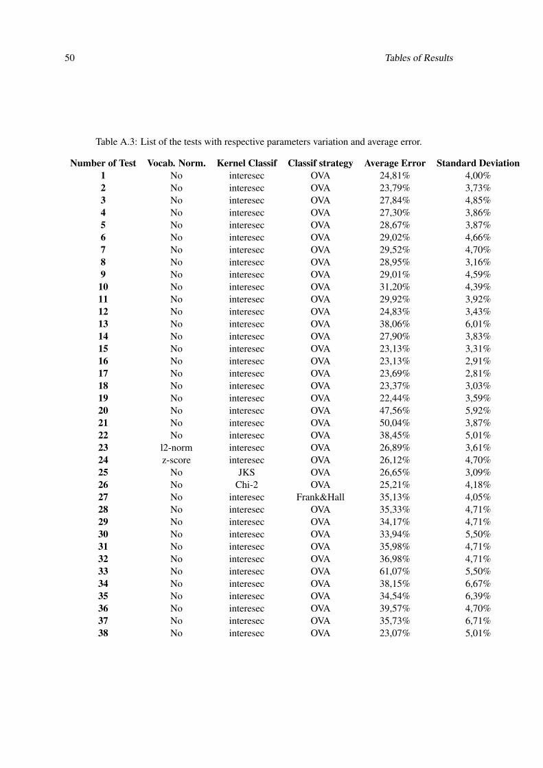
50 Tables of Results
Table A.3: List of the tests with respective parameters variation and average error.
Number of Test Vocab. Norm. Kernel Classif Classif strategy Average Error Standard Deviation1 No interesec OVA 24,81% 4,00%2 No interesec OVA 23,79% 3,73%3 No interesec OVA 27,84% 4,85%4 No interesec OVA 27,30% 3,86%5 No interesec OVA 28,67% 3,87%6 No interesec OVA 29,02% 4,66%7 No interesec OVA 29,52% 4,70%8 No interesec OVA 28,95% 3,16%9 No interesec OVA 29,01% 4,59%10 No interesec OVA 31,20% 4,39%11 No interesec OVA 29,92% 3,92%12 No interesec OVA 24,83% 3,43%13 No interesec OVA 38,06% 6,01%14 No interesec OVA 27,90% 3,83%15 No interesec OVA 23,13% 3,31%16 No interesec OVA 23,13% 2,91%17 No interesec OVA 23,69% 2,81%18 No interesec OVA 23,37% 3,03%19 No interesec OVA 22,44% 3,59%20 No interesec OVA 47,56% 5,92%21 No interesec OVA 50,04% 3,87%22 No interesec OVA 38,45% 5,01%23 l2-norm interesec OVA 26,89% 3,61%24 z-score interesec OVA 26,12% 4,70%25 No JKS OVA 26,65% 3,09%26 No Chi-2 OVA 25,21% 4,18%27 No interesec Frank&Hall 35,13% 4,05%28 No interesec OVA 35,33% 4,71%29 No interesec OVA 34,17% 4,71%30 No interesec OVA 33,94% 5,50%31 No interesec OVA 35,98% 4,71%32 No interesec OVA 36,98% 4,71%33 No interesec OVA 61,07% 5,50%34 No interesec OVA 38,15% 6,67%35 No interesec OVA 34,54% 6,39%36 No interesec OVA 39,57% 4,70%37 No interesec OVA 35,73% 6,71%38 No interesec OVA 23,07% 5,01%

Tables of Results 51
Table A.4: List of the tests with respective parameters variation and average error (continuation inTable A.5).
Test Color Patch Rotation Resizing Scale NumberName Size Information Scale of Patches
Patch + K-means grayscale 5x5 No 50% 100SIFT+RF grayscale 5x5 No 50% 100
SIFT+Kmeans grayscale 5x5 No 50% 100Leaf nodes grayscale 5x5 No 50% -
Table A.5: List of the tests with respective parameters variation and average error (continuation inTable A.6).
Test How choose Patches Number NumberName Parches Normalization of Trees of Nodes
Patch + K-means randomly l2-norm 10 100SIFT+RF randomly l2-norm 10 100
SIFT+Kmeans randomly l2-norm 10 100Leaf nodes randomly l2-norm 10 100
Table A.6: List of the tests with respective parameters variation and average error.
Test Vocabulary Kernel Classif Average StandardName Normalization Classif Strategy Error Deviation
Patch + K-means No interesec OVA 46,80% 9,82%SIFT+RF No interesec OVA 55,79% 7,40%
SIFT+Kmeans No interesec OVA 30,44% 4,20%Leaf nodes No interesec OVA 25,44% 5,03%

52 Tables of Results
Table A.7: Average error varying the number of trees of the RF and number of nodes for tree(continuation in Table A.8).
Number of Nodes10 50 100 200
Average SD Average SD Average SD Average SD
Number
1 61.07% 5.35% 25.88% 5.08% 26.32% 3.29% 26.57% 3.90%2 38.15% 10.01% 25.99% 3.95% 27.09% 3.86% 28.35% 2.86%3 28.62% 6.55% 25.19% 3.04% 27.10% 3.91% 27.26% 4.28%4 27.73% 8.11% 25.56% 3.98% 26.88% 4.56% 28.54% 4.55%5 24.78% 1.82% 23.95% 3.03% 24.96% 4.10% 25.29% 3.91%6 23.32% 4.25% 24.09% 4.42% 25.01% 4.32% 24.26% 4.15%7 26.29% 4.10% 26.18% 3.52% 25.75% 3.70% 25.57% 3.59%
of Trees
8 24.99% 3.34% 26.03% 3.73% 26.79% 4.55% 25.74% 3.68%9 24.04% 3.90% 24.99% 3.58% 24.32% 3.06% 23.76% 3.24%10 24.14% 2.80% 25.44% 3.87% 24.00% 3.75% 23.72% 3.87%50 25.63% 3.00% 23.96% 3.23% 23.85% 3.23% 23.63% 3.07%
100 25.63% 3.40% 24.06% 2.96% 23.51% 2.62% 23.22% 2.92%200 26.53% 4.04% 24.61% 2.90% 23.52% 3.26% 24.36% 2.88%300 26.75% 4.38% 24.61% 2,90% 24.42% 2.96% 23.89% 3.33%500 27.15% 4.29% 24.61% 2,90% 24.42% 2.96% 24.36% 2.88%
Table A.8: Average error varying the number of trees of the RF and number of nodes for tree.
Number of Nodes300 500 800 1000
Average SD Average SD Average SD Average SD
Number
1 27.26% 4.28% 27.94% 3.75% 28.82% 3.85% 28.38% 3.52%2 28.54% 4.55% 26.83% 3.04% 26.08% 3.00% 25.44% 3.06%3 25.29% 3.91% 26.48% 3.64% 25.49% 3.08% 25.40% 3.02%4 24.26% 4.15% 27.47% 4.59% 26.58% 4.27% 26.16% 3.46%5 25.57% 3.59% 23.71% 3.66% 23.69% 2.77% 23.39% 3.01%6 25.74% 3.68% 23.95% 4.45% 23.64% 4.71% 23.49% 4.66%7 23.76% 3.24% 24.80% 2.99% 24.82% 3.77% 24.87% 3.37%
of Nodes
8 23.72% 3.87% 25.18% 3.48% 25.14% 3.19% 25.31% 3.47%9 23.63% 3.07% 23.50% 3.59% 23.32% 2.91% 23.24% 2.81%10 23.22% 2.92% 24.38% 4.24% 23.90% 3.97% 23.71% 3.75%50 22.42% 2.72% 23.76% 2.57% 23.28% 2.88% 23.13% 3.04%100 23.89% 3.33% 23.15% 2.23% 22.67% 2.55% 22.63% 2.67%200 24.36% 2.88% 22.36% 2.84% 22.39% 2.74% 22.35% 2.89%300 24.36% 2.88% 23.13% 3.27% 23.12% 3.19% 23.51% 3.63%500 24.36% 2.88% 23.65% 2.63% 23.61% 2.64% 24.08% 2.63%

Appendix B
IJUP Abstract
The following page presents the abstract document submitted for the IJUP - Investigação Jovem
da Universidade do Porto. Additionally, a part of the work developed in the aim of this project
was exposed in IJUP 2015 in an oral presentation.
53

Recognition of Cancer using a Bag-of-Words Random Forest for Gastroenterology
S. Francisco1,2, Miguel T. Coimbra 2,5, R. Gamelas Sousa 3,4
1 Faculdade de Engenharia, Universidade do Porto, Portugal.
2 Instituto de Telecomunicações, Porto, Portugal. 3 Instituto de Investigação e Inovação em Saúde, Universidade do Porto, Portugal
4 Instituto de Engenharia Biomédica (INEB), Porto, Portugal 5 Faculdade de Ciências, Universidade do Porto, Portugal
In gastroenterology, Computer Aided Diagnosis techniques have allowed physicians to
analyze endoscopic images as a first or second opinion, or even as an educational
program [4]. Cancer recognition in the gastroenterology track is such a difficult problem
that only trained physicians can easily detect. Some pattern recognition solutions have
already been published in the past [1-4]. However, these solutions have to be invariant
to acquisition constraints (rotation, scale and luminance), goals which are not always
achieved.
We extract features from pre-processed endoscopic images, extracted pixel intensities of
some regions, and then use Random Forests to create a Bag of Feature Words (BoW).
The BoW is built by counting how many times each feature appears on each image, thus
giving its information content, and used to build a classification model using Support
Vector Machines.
Our dataset 176 chromoendoscopy images of the oesophagus (30 for training and the
remainder for testing), exhibiting three different conditions (normal and the pathological
tissues with dysplasia and metaplasia). After 50 runs, we achieve 22.03±3.09% of
average error. This results are promissory, especially when compared to the usage of
SIFT descriptor and k-means (32.20±3.58%) to generate the BoW for classification.
Our methodology seems to deal well with few data train samples and it is statistically
different and better then the results of the existent methodologies.
References:
[1] Sousa, R et al.., Moura, D.C., Ribeiro, M.D. and Coimbra, M.T. (2014), Local self similar
descriptors: Comparison and application to gastroenterology images, Engineering in Medicine
and Biology Society (EMBC), pp. 4635-4638.
[2] Riaz, F. et al., Silva, F.B., Ribeiro, M.D., and Coimbra, M.T. (2012), Invariant gabor texture
descriptors for classification of gastroenterology images, Biomedical Engineering, IEEE
Transactions, v. 59, n. 10, pp. 2893-2904.
[3] Gross, S., Trautwein, C., Behrens, A., Winograd, R., Palm, S., Lutz, H.H., Sokhan, R.S.,
Hecker, H., Aach, T. and Tischendorf J.J.W.et al. (2011), Computer-based classification of
small colorectal polyps by using narrow-band imaging with optical magnification,
Gastrointestinal endoscopy 74.6, pp. 1354-1359.
[4] Balbaque, F.S., Ribeiro, M.D., Rabenstein, T., Goda, K., Kiesslich, R., Harigsma, J., Edebo,
A., Toth, E., Soares, J., Areia, M., Lundell, L. and Marschall, H.U. et al.(2013), Endoscopic
assessment and grading of Barrett's esophagus using magnification endoscopy and narrow
band imaging: Impact of structured learning and experience on the accuracy of the Amsterdam
classification system, Scandinavian journal of gastroenterology, v. 48, n. 2, pp. 160-167.

Appendix C
Summary Paper
The following pages present the two-pages summary paper of this Dissertation. It is also available
in http://sarafranciscothesis.pt.vu/.
55
PROVAS DE DISSERTACAO DO MEB —JULHO DE 2015 1
Recognition of Cancer using Random Forests as aBag-of-Words Approach for Gastroenterology
Sara Francisco∗ Ricardo G. Sousa (orientador)† Miguel T. Coimbra (co-orientador)‡
Resumo—Recognition of cancer in gastroenterology (GE) ima-ges is a challenging task, in which only trained physicianssucceed. Computer Aided Diagnosis systems have been applyingpattern recognition strategies in this context to act as a first orsecond opinion to help physicians. However, such solutions areself-tailored and affected by image acquisition constraints. Wepropose a methodology that automatically renders representativefeatures for gastroenterology images from a Bag of Words (BoW)generated with Random Forests (RF). Our experimental studyis made over a multiclass dataset of chromoendoscopy images.An optimal average error of 23.07± 2.83% was obtained, whilekeeping the computational time low, suggesting usability in amedical context and outperforming the standard approaches inthis application.
Index Terms—Bag-of-Words, Computer Vision, Endoscopy,Random Forests
I. INTRODUCTION
EVERY year, 2.8 million people are diagnosed with cancerin the gastrointestinal tract and around 1.8 million die
of it. Recent studies have shown that the survival rates areespecially high for early diagnosis of this cancer, motivatingthe search for novel, objective and quantitative methods to helpmedical teams on this task. Computer Vision (CV) solutionshave been applied to the classification of endoscopic imageswith usefulness, adding a quantitative evaluation to the well-established, accurate and minimally invasive endoscopic pro-cedure. However, the endoscopic image acquisition is affectedby several constraints which difficult the recognition of cancerrecognition and reduce the applicability of some of those CVmethodologies.
Currently, the classification of GE images is done byextracting distinctive features from the images, either onthe frequency domain (i.e., Gabor filters) or in the spatialdomain (i.e., SIFT descriptor), and feeding it to classifica-tion models using Support Vector Machines (SVM) or k-NN. Although presenting promising results, such methods canstill be improved in terms of descriptiveness and accuracy.Additionally, it would be important to dismiss the need for anuser to tune the algorithm parameters, making its definitionautomatic and adaptable to new datasets. For that, in thiswork we extend recent advances in CV to the analysis ofGE images. Such approaches are commonly used to recognizeobjects in cluttered scenes by creating a (sparse) histogramof occurrences (vocabulary) of each different pattern (visualword) in the images. A set of visual words is known as BoW
∗ [email protected]† Post-Doctoral Researcher, I3S, INEB, [email protected]‡ Auxiliary Professor, FCUP, IT, [email protected]
and describes the content and frequency of each pattern on animage. This introduces new information to the analysis: notonly we know which patterns occur, but also how many timesand how different they are.
Different approaches can be used to generate a BoW of theinput data. Here, we propose the usage of RF to perform anhierarchical clustering of input pixel-intensities towards thecreation of a BoW, in which each visual word correspondsto a unique and distinct pattern on the endoscopic image. ARF is an ensemble of Decision Trees (DT). DT are statisticalapproaches designed for decision support strategies. They takethe input data and subject it to a sequence of binary decisions.This sequence is an iterative approach of sub-decisions thatpartition the feature space. With a single DT the differentpatterns of the data are not correctly learned [1]. However,using RF, we add randomization to the learning process andimprove the probability to have a more reliable model. RF havebeen applied to generate BoW by [2], however their usage inGE has not been studied yet. A similar approach has alreadybeen tested in GE by [3], but using SIFT and k-means togenerate the BoW.
II. METHODOLOGY
In this section, we describe the proposed processing pipeline(presented in Figure 1) for the analysis and classification ofGE images. The pivotal stage of our method consist in theconstruction of a vocabulary of the input data, using a BoWcreated from input pixel intensities using RF.
Figura 1: Overview of the pipeline of our methodology tobuild a classifier model for gastroenterology images.
A. Image Acquisition and Processing
Endoscopic images are acquired during an examination ofthe inner cavities of the gastric channel, and regions of interest(ROI) are delimited by physicians. For denoising purposes,images are resized and smoothed using a Gaussian low-pass

PROVAS DE DISSERTACAO DO MEB —JULHO DE 2015 2
filter. Then, we subdivide the ROI into patches of differentsizes containing the pixel intensities of the image.
B. Visual Representation
We generate a BoW using RF. Here, each patch descendseach of the decision trees on the forest, until a leaf nodeis reached. We repeat this process to all of the trees andpatches and count the number of times each node belongs to adescending path, resulting in the vocabulary, our representationof the images from which we construct the classifier. Thevocabulary can be perceived as an histogram of the visualwords and quantize the occurrence of each pattern in theimage.
C. Image Recognition
We use SVM to classify the images. The classification mo-del is generated by supervised learning and cost parameters aredefined by 3-folds Cross-Validation. Since we are are dealingwith a multiclass problem, with different cancer stages (normaltissues, tissues with metaplasia and tissues with displasia), weapplied a One-versus-All (OVA) strategy.
III. RESULTS AND DISCUSSION
A. Dataset
Our dataset consisted of 176 chromoendoscopic images,pre-segmentated into clinically relevant regions, according tomanual annotations by an expert physician. This dataset isencompassed by 56 normal tissues and 96 metaplasia and 24dysplasia cases (see [4] for more information).
B. Image Processing and Information Extraction
Conversion to grayscale lead to lower errors when comparedto RGB, Opponent Space and CIE-lab conversions. ExistingCV techniques for image classification cannot assess relevantcolor information [5], which may explain the results. Theinfluence of patch width and number were tested. The bestperformances were obtained for small patch widths, 5 × 5,and 200 patches, randomly chosen. These results suggest thatwe were able capture the pattern diversity on the images withlow computational cost. Small portions of the input data, ran-domly chosen and without incorporating rotation information,provide a reliable general description of the image. We studiedthe influence of patch normalization and concluded that L2-normalization lead to better results.
C. Random Forests
The vocabulary dimension and the performance of ourmethodology is highly influenced by the number of nodes pertree and the number of trees of the RF. The best performancewas found for 50 trees, with 300 nodes each, guaranteeingenough randomness on the forest to capture the pattern diver-sity on the images, and an intermediate number of nodes toavoid redundant branches when a patch descends a tree. Suchevidence is shown in Figure 2. Better results were obtainedwhen the vocabulary was not normalized.
0 200 400 600 800 1,0000
0.2
0.4
Number of Nodes
Ave
rage
Err
or
50 Trees
0 200 400 600 800 1,0000
0.2
0.4
Number of Nodes
Ave
rage
Err
or
2 Trees
Figura 2: Average error variation for different number of nodesand trees.
D. Recognition of cancerThe intersection kernel of the input data was also found to
perform slightly better than χ2 and JKS kernels [6]. The inputdata is seen as histograms, making an operation of similarityof histograms potentially better
E. Whole MethodologyWe compared the methodology here proposed using the best
parametrization with the methodology presented by [3], whichuses standard feature extraction and BoW generation methods(respectively, patch extraction and RF versus SIFT and k-means). We obtained a 23.79± 3.70% average error, versus a30.44± 4.20% average error using the standard methodology.The results suggest that our methodology is competitive,especially taking into consideration that each new input imageneeds around 5 seconds to be classified, allowing near real-time feedback to physicians with reliability. Furthermore, weeliminated the distinction between metaplasia and displasia,and assessed the cancer recognition using only normal andpathological tissues. An average error of 11.03 ± 1.80% wasobtained.
IV. CONCLUSIONS
We developed a new methodology that explores the hie-rarchical clustering capacity of RF to generate a BoW andclassify GE images. We improved upon the standard metho-dologies for cancer recognition in this context, with a lowaverage error of classification and low processing time foreach new image.
REFERENCES
[1] J. Friedman, T. Hastie, and R. Tibshirani, The elements of statisticallearning. Springer series in statistics Springer, Berlin, 2001, vol. 1.
[2] J. Shotton, M. Johnson, and R. Cipolla, “Semantic texton forests forimage categorization and segmentation,” in Computer vision and patternrecognition, 2008. CVPR 2008. IEEE Conference on. IEEE, 2008, pp.1–8.
[3] R. Sousa, D. C. Moura, M. Dinis-Ribeiro, and M. T. Coimbra, “Localself similar descriptors: Comparison and application to gastroenterologyimages,” in Engineering in Medicine and Biology Society (EMBC), 201436th Annual International Conference of the IEEE. IEEE, 2014, pp.4635–4638.
[4] M. Dinis-Ribeiro, A. da Costa-Pereira, C. Lopes, L. Lara-Santos, M. Gui-lherme, L. Moreira-Dias, H. Lomba-Viana, A. Ribeiro, C. Santos, J. So-ares et al., “Magnification chromoendoscopy for the diagnosis of gastricintestinal metaplasia and dysplasia,” Gastrointestinal endoscopy, vol. 57,no. 4, pp. 498–504, 2003.
[5] F. Riaz, F. B. Silva, M. D. Ribeiro, and M. T. Coimbra, “Impact of visualfeatures on the segmentation of gastroenterology images using normalizedcuts,” Biomedical Engineering, IEEE Transactions on, vol. 60, no. 5, pp.1191–1201, 2013.
[6] A. Vedaldi and A. Zisserman, “Efficient additive kernels via explicit fea-ture maps,” Pattern Analysis and Machine Intelligence, IEEE Transactionson, vol. 34, no. 3, pp. 480–492, 2012.


Bibliography
[1] Tomas Akenine-Möller, Eric Haines, and Naty Hoffman. Real-time rendering. CRC Press, 2008.[2] Miguel Areia, Rita Carvalho, Ana Teresa Cadime, Francisco Rocha Gonçalves, and Mário Dinis-Ribeiro. Screen-
ing for gastric cancer and surveillance of premalignant lesions: a systematic review of cost-effectiveness studies.Helicobacter, 18(5):325–337, 2013.
[3] G Berci and KA Forde. History of endoscopy. Surgical endoscopy, 14(1):5–15, 2000.[4] Christopher M Bishop et al. Pattern recognition and machine learning, volume 4. springer New York, 2006.[5] D Boswell. Introduction to support vector machines: University of carlifornia. San Diego, 2002.[6] Ken Chatfield, Victor Lempitsky, Andrea Vedaldi, and Andrew Zisserman. The devil is in the details: an evalua-
tion of recent feature encoding methods. 2011.[7] R Coriat, A Chryssostalis, JD Zeitoun, J Deyra, M Gaudric, F Prat, and S Chaussade. Computed virtual chro-
moendoscopy system (fice): a new tool for upper endoscopy? Gastroentérologie clinique et biologique, 32(4):363–369, 2008.
[8] James L Crowley and Alice C Parker. A representation for shape based on peaks and ridges in the difference oflow-pass transform. Pattern Analysis and Machine Intelligence, IEEE Transactions on, (2):156–170, 1984.
[9] Gabriella Csurka, Christopher Dance, Lixin Fan, Jutta Willamowski, and Cédric Bray. Visual categorization withbags of keypoints. In Workshop on statistical learning in computer vision, ECCV, volume 1, pages 1–2. Prague,2004.
[10] Wouter L Curvers, Lorenza Alvarez Herrero, Michael B Wallace, Louis-Michel Wong Kee Song, Krish Ragunath,Herbert C Wolfsen, Ganapathy A Prasad, Kenneth K Wang, Venkataraman Subramanian, Bas LAM Weusten, et al.Endoscopic tri-modal imaging is more effective than standard endoscopy in identifying early-stage neoplasia inbarrett’s esophagus. Gastroenterology, 139(4):1106–1114, 2010.
[11] M Dhanalakshmi, N Sriraam, G Ramya, N Bhargavi, and V Tamizhtennagaarasi. Computer aided diagnosis forenteric lesions in endoscopic images using anfis. International Journal of Wisdom Based Computing, 2(1), 2012.
[12] Mário Dinis-Ribeiro, Altamiro da Costa-Pereira, Carlos Lopes, Lúcio Lara-Santos, Mateus Guilherme, LuísMoreira-Dias, Helena Lomba-Viana, Armando Ribeiro, Costa Santos, José Soares, et al. Magnification chro-moendoscopy for the diagnosis of gastric intestinal metaplasia and dysplasia. Gastrointestinal endoscopy, 57(4):498–504, 2003.
[13] Jacques Ferlay, Isabelle Soerjomataram, Rajesh Dikshit, Sultan Eser, Colin Mathers, Marise Rebelo, Don-ald Maxwell Parkin, David Forman, and Freddie Bray. Cancer incidence and mortality worldwide: sources,methods and major patterns in globocan 2012. International Journal of Cancer, 2014.
[14] Eibe Frank and Mark Hall. A simple approach to ordinal classification. Springer, 2001.[15] Jerome Friedman, Trevor Hastie, and Robert Tibshirani. The elements of statistical learning, volume 1. Springer
series in statistics Springer, Berlin, 2001.[16] Mikihiro Fujiya, Kentaro Moriichi, Nobuhiro Ueno, Yusuke Saitoh, and Yutaka Kohgo. Autofluorescence imaging
for diagnosing intestinal disorders. Colonocopy/Book, 1, 2011.[17] Dennis Gabor. Theory of communication. part 1: The analysis of information. Journal of the Institution of
Electrical Engineers-Part III: Radio and Communication Engineering, 93(26):429–441, 1946.[18] Sebastian Gross, Thomas Stehle, Alexander Behrens, Roland Auer, Til Aach, Ron Winograd, Christian Trautwein,
and Jens Tischendorf. A comparison of blood vessel features and local binary patterns for colorectal polypclassification. In SPIE Medical Imaging, pages 72602Q–72602Q. International Society for Optics and Photonics,2009.
[19] Michael Haefner, Leonhard Brunauer, Hannes Payer, Robert Resch, Alfred Gangl, Andreas Uhl, Friedrich Wrba,and Andreas Vécsei. Computer-aided classification of zoom-endoscopical images using fourier filters. Informa-tion Technology in Biomedicine, IEEE Transactions on, 14(4):958–970, 2010.
[20] Michael Häfner, Alfred Gangl, Michael Liedlgruber, Andreas Uhl, Andreas Vécsei, and Friedrich Wrba. Classi-fication of endoscopic images using delaunay triangulation-based edge features. In Image Analysis and Recogni-tion, pages 131–140. Springer, 2010.
59

60 BIBLIOGRAPHY
[21] Rehan Haidry and Laurence Lovat. Medical Imaging in Clinical Practice: Novel Imaging Techniques in Gas-trointestinal Endoscopy in the Upper Gastrointestinal Tract. InTech Open, 2013.
[22] Robert M Haralick, Karthikeyan Shanmugam, and Its’ Hak Dinstein. Textural features for image classification.Systems, Man and Cybernetics, IEEE Transactions on, (6):610–621, 1973.
[23] Chris Harris and Mike Stephens. A combined corner and edge detector. In Alvey vision conference, volume 15,page 50. Manchester, UK, 1988.
[24] Sebastian Hegenbart, Andreas Uhl, Andreas Vécsei, and Georg Wimmer. Scale invariant texture descriptors forclassifying celiac disease. Medical image analysis, 17(4):458–474, 2013.
[25] Janusz AZ Jankowski and Ernest T Hawk. Handbook of Gastrointestinal Cancer. Wiley Online Library, 2013.[26] Carlos M Jarque and Anil K Bera. Efficient tests for normality, homoscedasticity and serial independence of
regression residuals. Economics letters, 6(3):255–259, 1980.[27] Yulei Jiang, Robert M Nishikawa, Robert A Schmidt, Charles E Metz, Maryellen L Giger, and Kunio Doi. Im-
proving breast cancer diagnosis with computer-aided diagnosis. Academic radiology, 6(1):22–33, 1999.[28] Cyrus R Kapadia. Gastric atrophy, metaplasia, and dysplasia: a clinical perspective. Journal of clinical gastroen-
terology, 36(5):S29–S36, 2003.[29] Hiroyuki Kodama, Fumihiko Yano, Satoki P Ninomija, Y Sakai, and S Ninomiya. A digital imaging processing
method for gastric endoscope picture. In System Sciences, 1988. Vol. IV. Applications Track., Proceedings of theTwenty-First Annual Hawaii International Conference on, volume 4, pages 277–282. IEEE, 1988.
[30] Shinya Kodashima and Mitsuhiro Fujishiro. Novel image-enhanced endoscopy with i-scan technology. Worldjournal of gastroenterology: WJG, 16(9):1043, 2010.
[31] Wen-Jia Kuo, Ruey-Feng Chang, Woo Kyung Moon, Cheng Chun Lee, and Dar-Ren Chen. Computer-aideddiagnosis of breast tumors with different us systems. Academic radiology, 9(7):793–799, 2002.
[32] Hoo-Yeon Lee, Eun-Cheol Park, Jae Kwan Jun, Kui Son Choi, and Myung-Il Hahm. Comparing upper gastroin-testinal x-ray and endoscopy for gastric cancer diagnosis in korea. World Journal of Gastroenterology, 16(2):245,2010.
[33] Baopu Li and MQ-H Meng. Tumor recognition in wireless capsule endoscopy images using textural featuresand svm-based feature selection. Information Technology in Biomedicine, IEEE Transactions on, 16(3):323–329,2012.
[34] Michael Liedlgruber and Andreas Uhl. Computer-aided decision support systems for endoscopy in the gastroin-testinal tract: A review. IEEE reviews in biomedical engineering, 4:73–88, 2011.
[35] David G Lowe. Distinctive image features from scale-invariant keypoints. International journal of computervision, 60(2):91–110, 2004.
[36] J Mannath, V Subramanian, CJ Hawkey, and K Ragunath. Narrow band imaging for characterization of highgrade dysplasia and specialized intestinal metaplasia in barrett’s esophagus: a meta-analysis. Endoscopy, 42(05):351–359, 2010.
[37] Frank Moosmann, Bill Triggs, and Frederic Jurie. Fast discriminative visual codebooks using randomized clus-tering forests. In 20th Annual Conference on Neural Information Processing Systems (NIPS’06), pages 985–992.MIT Press, 2007.
[38] Ruwan Nawarathna, JungHwan Oh, Jayantha Muthukudage, Wallapak Tavanapong, Johnny Wong, Piet CDe Groen, and Shou Jiang Tang. Abnormal image detection in endoscopy videos using a filter bank and lo-cal binary patterns. Neurocomputing, 144:70–91, 2014.
[39] Nagaaki Ohyama, Hirohisa Machida, Kazuhiro Gono, Takashi Obi, Yasuo Hamamoto, Takao Endo, MasahiroYamaguchi, Yasushi Sano, and Shigeaki Yoshida. Appearance of enhanced tissue features in narrow-band endo-scopic imaging. Journal of biomedical optics, 9(3):568–577, 2004.
[40] Timo Ojala, Matti Pietikainen, and David Harwood. Performance evaluation of texture measures with classi-fication based on kullback discrimination of distributions. In Pattern Recognition, 1994. Vol. 1-Conference A:Computer Vision & Image Processing., Proceedings of the 12th IAPR International Conference on, vol-ume 1, pages 582–585. IEEE, 1994.
[41] Keiichi Onji, Shigeto Yoshida, Shinji Tanaka, Rie Kawase, Yoshito Takemura, Shiro Oka, Toru Tamaki, BisserRaytchev, Kazufumi Kaneda, Masaharu Yoshihara, et al. Quantitative analysis of colorectal lesions observed onmagnified endoscopy images. Journal of gastroenterology, 46(12):1382–1390, 2011.
[42] Konstantinos N Plataniotis and Anastasios N Venetsanopoulos. Color image processing and applications.Springer Science & Business Media, 2000.
[43] I Rácz and E Tóth. [chromoendoscopic study of the gastric mucosa]. Orvosi hetilap, 130(49):2635–2638, 1989.[44] Farhan Riaz, Francisco Baldaque Silva, Mario Dinis Ribeiro, and Miguel Tavares Coimbra. Invariant gabor
texture descriptors for classification of gastroenterology images. Biomedical Engineering, IEEE Transactions on,59(10):2893–2904, 2012.
[45] Farhan Riaz, Francisco Baldaque Silva, Mario Dinis Ribeiro, and Miguel Tavares Coimbra. Impact of visualfeatures on the segmentation of gastroenterology images using normalized cuts. Biomedical Engineering, IEEETransactions on, 60(5):1191–1201, 2013.

BIBLIOGRAPHY 61
[46] Lior Rokach. Fuzzy decision trees. 2008.[47] R.R. Seeley, P. Tate, and T.D. Stephens. Anatomy and Physiology. McGraw-Hill Higher Education, 2007. ISBN
9780073293684.[48] Jamie Shotton, Matthew Johnson, and Roberto Cipolla. Semantic texton forests for image categorization and
segmentation. In Computer vision and pattern recognition, 2008. CVPR 2008. IEEE Conference on, pages 1–8.IEEE, 2008.
[49] MD Shui-Yi Tung, Cheng-Shyong Wu, and Ming-Yao Su. Magnifying colonoscopy in differentiating neoplasticfrom nonneoplastic colorectal lesions. The American journal of gastroenterology, 96:2628–2632, 2001.
[50] Rebecca Siegel, Jiemin Ma, Zhaohui Zou, and Ahmedin Jemal. Cancer statistics, 2014. CA: a cancer journal forclinicians, 64(1):9–29, 2014.
[51] Karen Simonyan, Andrea Vedaldi, and Andrew Zisserman. Descriptor learning using convex optimisation. Com-puter Vision–ECCV 2012, pages 243–256, 2012.
[52] R. Singh, GK Anagnostopoulos, K. Yao, H. Karageorgiou, PJ Fortun, A. Shonde, K. Garsed, PV Kaye,CJ Hawkey, K. Ragunath, et al. Narrow-band imaging with magnification in barrett’s esophagus: validationof a simplified grading system of mucosal morphology patterns against histology. Endoscopy, 40(6):457, 2008.
[53] Rajvinder Singh, SweeLin Chen Yi Mei, and Sandeep Sethi. Advanced endoscopic imaging in barrett’s oesopha-gus: A review on current practice. World journal of gastroenterology: WJG, 17(38):4271, 2011.
[54] MV Sivak. Gastrointestinal endoscopy: past and future. Gut, 55(8):1061–1064, 2006.[55] Stephen M Smith and J Michael Brady. Susan—a new approach to low level image processing. International
journal of computer vision, 23(1):45–78, 1997.[56] Louis-Michel Wong Kee Song and Brian C Wilson. Endoscopic detection of early upper gi cancers. Best Practice
& Research Clinical Gastroenterology, 19(6):833–856, 2005.[57] Ricardo Sousa, Mario-Dinis Ribeiro, Pedro Pimentel-Nunes, and Miguel Tavares Coimbra. Impact of svm multi-
class decomposition rules for recognition of cancer in gastroenterology images. pages 405–408, 2013.[58] Ricardo Sousa, Daniel C Moura, Mario Dinis-Ribeiro, and Miguel T Coimbra. Local self similar descrip-
tors: Comparison and application to gastroenterology images. In Engineering in Medicine and Biology Society(EMBC), 2014 36th Annual International Conference of the IEEE, pages 4635–4638. IEEE, 2014.
[59] Peter D Stevens, Charles J Lightdale, PH Green, Lance M Siegel, Reuben J Garcia-Carrasquillo, and HeidrunRotterdam. Combined magnification endoscopy with chromoendoscopy for the evaluation of barrett’s esophagus.Gastrointestinal endoscopy, 40(6):747, 1994.
[60] Venkataraman Subramanian and Krish Ragunath. Advanced endoscopic imaging: a review of commerciallyavailable technologies. Clinical Gastroenterology and Hepatology, 12(3):368–376, 2014.
[61] Xiaoyang Tan and Bill Triggs. Enhanced local texture feature sets for face recognition under difficult lightingconditions. Image Processing, IEEE Transactions on, 19(6):1635–1650, 2010.
[62] Thorsten Thadewald and Herbert Büning. Jarque–bera test and its competitors for testing normality–a powercomparison. Journal of Applied Statistics, 34(1):87–105, 2007.
[63] JJW Tischendorf, S Gross, R Winograd, H Hecker, R Auer, A Behrens, C Trautwein, T Aach, and T Stehle.Computer-aided classification of colorectal polyps based on vascular patterns: a pilot study. Endoscopy, 42(03):203–207, 2010.
[64] Tomasz Trzcinski, Mario Christoudias, Vincent Lepetit, and Pascal Fua. Learning image descriptors with theboosting-trick. In Advances in neural information processing systems, pages 269–277, 2012.
[65] Tinne Tuytelaars and Krystian Mikolajczyk. Local invariant feature detectors: a survey. Foundations andTrends R© in Computer Graphics and Vision, 3(3):177–280, 2008.
[66] Vladimir Naumovich Vapnik and Vlamimir Vapnik. Statistical learning theory, volume 1. Wiley New York,1998.
[67] Andreas Vécsei, Thomas Fuhrmann, Michael Liedlgruber, Leonhard Brunauer, Hannes Payer, and Andreas Uhl.Automated classification of duodenal imagery in celiac disease using evolved fourier feature vectors. Computermethods and programs in biomedicine, 95(2):S68–S78, 2009.
[68] Julia Vogel and Bernt Schiele. A semantic typicality measure for natural scene categorization. In Pattern Recog-nition, pages 195–203. Springer, 2004.
[69] Dag Wormanns, Martin Fiebich, Mustafa Saidi, Stefan Diederich, and Walter Heindel. Automatic detection ofpulmonary nodules at spiral ct: clinical application of a computer-aided diagnosis system. European radiology,12(5):1052–1057, 2002.
[70] Bangpeng Yao, Aditya Khosla, and Li Fei-Fei. Combining randomization and discrimination for fine-grainedimage categorization. In Computer Vision and Pattern Recognition (CVPR), 2011 IEEE Conference on, pages1577–1584. IEEE, 2011.
[71] Naohisa Yoshida, Nobuaki Yagi, Yutaka Inada, Munehiro Kugai, Akio Yanagisawa, and Yuji Naito. Therapeuticand diagnostic approaches in colonoscopy. 2013.
[72] KC Yuan. Gastrointestinal cancer. Journal of Gastrointestinal and Digestive System, 3(125):2, 2013.

62 BIBLIOGRAPHY
[73] Barbara Zitova and Jan Flusser. Image registration methods: a survey. Image and vision computing, 21(11):977–1000, 2003.