Reciprocal Space Mapping for Dummies
24
1 Reciprocal Space Mapping for Dummies Samuele Lilliu 1 , Thomas Dane 2 1 University of Sheffield, Hicks Building, Hounsfield Road, Sheffield, S3 7RH (UK), 2 European Synchrotron Radiation Facility, BP 220, Grenoble F-38043, France. Abstract Grazing Incidence X-ray Diffraction (GIXD) is a surface sensitive X-ray investigation technique (or geometry configuration) that can reveal the structural properties of a film deposited on a flat substrate 1-4 . The term grazing indicates that the angle between the incident beam and the film is small (typically below 0.5°). This essential technique has been employed on liquid crystals 5,6 , nanoparticles and colloids 7,8 , nanostructures 9 , corrosion processes 10,11 , polymers 12-14 , bio-materials 15-17 , interfaces 11,18 , materials for solar cells 19-25 , photodiodes 26 , and transistors 27,28 , etc. Diffraction patterns in GIXD geometry are typically captured with a 2D detector, which outputs images in pixel coordinates. A step required to perform analyses such as grain size estimation, disorder, preferred orientation, quantitative phase analysis of the probed film surface, etc. 29 , consists in converting the diffraction image from pixel coordinates to the momentum transfer or scattering vector in sample coordinates (the ‘reciprocal space mapping’) 30 . This momentum transfer embeds information on the crystal or polycrystal and its intrinsic rotation with respect to the substrate. In this work we derive, in a rigorous way, the reciprocal space mapping equations for a ‘3D+1S’ diffractometer in a way that is understandable to anyone with basic notions of linear algebra, geometry, and X-ray diffraction. Introduction Two-dimensional X-ray diffraction (XRD 2 ) is a well-established technique in the field of X-ray diffraction (XRD) 29 . The main complication of data analysis in XRD 2 compared to one dimension XRD is the remapping of detector pixel coordinates into momentum transfer or scattering vector coordinates. The geometry of a two-dimensional X-ray diffraction system consists of three reference systems: laboratory, detector, and sample. The laboratory coordinate system is the reference or global three dimensional coordinate system. The sample coordinate system shares the same origin with the laboratory system but its basis can be oriented in a different way. The detector coordinates system is two-dimensional. The three reference systems are represented by orthogonal Cartesian basis 31-34 . In this work we employ a ‘3D+1S’ diffractometer, where three diffractometer circles (3D) are used for moving the 2D detector across the Ewald sphere, and one circle is used for orienting the sample. The simplest detector orientation corresponds to the situation in which the normal to the detector is coincident to the X-ray incident beam or, equivalently, points towards the origin of the laboratory coordinate system, where the sample is placed (detector circle angles are zero). The simplest sample orientation corresponds to the grazing case in which the sample surface is parallel to the direct beam (sample circle angle is zero). Let’s assume that our sample is a powder of randomly oriented crystals and consider a diffracting plane. The diffracting plane would project a cone of rays (Debye-Scherrer ring) onto the detector 1 . Since the detector is perpendicular to incident beam and the sample is parallel to the incident beam, the projection of the diffracting cone onto the detector would be a perfect circle. In this case, converting detector’s pixel coordinates into scattering vector coordinates is non-trivial. However one might want to move the detector to non-zero azimuth and elevation to visualize extra Debye-Scherrer rings. This complicates things and introduces distortions in the diffraction pattern. In the most general case the Debye-Scherrer rings will have a tilted ellipse shape, which result from the intersection of the diffracting cone with the tilted detector plane. In this case, the conversion between pixels and scattering vector coordinates is more complicated.
Transcript of Reciprocal Space Mapping for Dummies

1
Reciprocal Space Mapping for Dummies
Samuele Lilliu1, Thomas Dane2
1University of Sheffield, Hicks Building, Hounsfield Road, Sheffield, S3 7RH (UK), 2European Synchrotron Radiation Facility, BP 220, Grenoble F-38043, France.
Abstract Grazing Incidence X-ray Diffraction (GIXD) is a surface sensitive X-ray investigation technique (or geometry configuration) that can reveal the structural properties of a film deposited on a flat substrate1-4. The term grazing indicates that the angle between the incident beam and the film is small (typically below 0.5°). This essential technique has been employed on liquid crystals5,6, nanoparticles and colloids7,8, nanostructures9, corrosion processes10,11, polymers12-14, bio-materials15-17, interfaces11,18, materials for solar cells19-25, photodiodes26, and transistors27,28, etc. Diffraction patterns in GIXD geometry are typically captured with a 2D detector, which outputs images in pixel coordinates. A step required to perform analyses such as grain size estimation, disorder, preferred orientation, quantitative phase analysis of the probed film surface, etc.29, consists in converting the diffraction image from pixel coordinates to the momentum transfer or scattering vector in sample coordinates (the ‘reciprocal space mapping’)30. This momentum transfer embeds information on the crystal or polycrystal and its intrinsic rotation with respect to the substrate. In this work we derive, in a rigorous way, the reciprocal space mapping equations for a ‘3D+1S’ diffractometer in a way that is understandable to anyone with basic notions of linear algebra, geometry, and X-ray diffraction.
Introduction Two-dimensional X-ray diffraction (XRD2) is a well-established technique in the field of X-ray diffraction (XRD)29. The main complication of data analysis in XRD2 compared to one dimension XRD is the remapping of detector pixel coordinates into momentum transfer or scattering vector coordinates. The geometry of a two-dimensional X-ray diffraction system consists of three reference systems: laboratory, detector, and sample. The laboratory coordinate system is the reference or global three dimensional coordinate system. The sample coordinate system shares the same origin with the laboratory system but its basis can be oriented in a different way. The detector coordinates system is two-dimensional. The three reference systems are represented by orthogonal Cartesian basis31-34.
In this work we employ a ‘3D+1S’ diffractometer, where three diffractometer circles (3D) are used for moving the 2D detector across the Ewald sphere, and one circle is used for orienting the sample. The simplest detector orientation corresponds to the situation in which the normal to the detector is coincident to the X-ray incident beam or, equivalently, points towards the origin of the laboratory coordinate system, where the sample is placed (detector circle angles are zero). The simplest sample orientation corresponds to the grazing case in which the sample surface is parallel to the direct beam (sample circle angle is zero). Let’s assume that our sample is a powder of randomly oriented crystals and consider a diffracting plane. The diffracting plane would project a cone of rays (Debye-Scherrer ring) onto the detector1. Since the detector is perpendicular to incident beam and the sample is parallel to the incident beam, the projection of the diffracting cone onto the detector would be a perfect circle. In this case, converting detector’s pixel coordinates into scattering vector coordinates is non-trivial. However one might want to move the detector to non-zero azimuth and elevation to visualize extra Debye-Scherrer rings. This complicates things and introduces distortions in the diffraction pattern. In the most general case the Debye-Scherrer rings will have a tilted ellipse shape, which result from the intersection of the diffracting cone with the tilted detector plane. In this case, the conversion between pixels and scattering vector coordinates is more complicated.
2
We start our discussion by introducing the diffractometer geometry and the laboratory coordinate system. We then show how to construct the rotation matrices for the detector rotation (3D). The next step is to project a generic ray onto a rotated detector. The projected ray is converted into the two-dimensional detector coordinates. At this point we have a set of equations that convert a generic ray into an image point. These equations can be inverted so that, given an image point, we can retrieve the ray information. Once we have extracted the inverted equations, we can specify the nature of the
ray as the exit wave versor �̂�𝑓. The scattering vector can be easily derived from �̂�𝑓. We then introduce
the effect of the rotation of one sample circle and derive the equations required to reconstruct the scattering vector in sample coordinates, which contains information on the crystal and its intrinsic rotation with respect to the substrate.
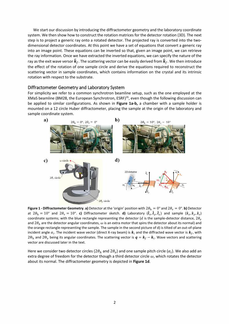
Diffractometer Geometry and Laboratory System For simplicity we refer to a common synchrotron beamline setup, such as the one employed at the XMaS beamline (BM28, the European Synchrotron, ESRF)35, even though the following discussion can be applied to similar configurations. As shown in Figure 1a-b, a chamber with a sample holder is mounted on a 12 circle Huber diffractometer, placing the sample at the origin of the laboratory and sample coordinate system.
Figure 1 - Diffractometer Geometry. a) Detector at the ‘origin’ position with 2𝜃h = 0° and 2𝜃v = 0°. b) Detector
at 2𝜃h = 10° and 2𝜃v = 10°. c) Diffractometer sketch. d) Laboratory (�̂�𝑥, �̂�𝑦 , �̂�𝑧) and sample (�̂�𝑥, �̂�𝑦 , �̂�𝑧)
coordinate systems; with the blue rectangle representing the detector (𝑑 is the sample-detector distance, 2𝜃𝑣 and 2𝜃ℎ are the detector angular coordinates, 𝜔 is an extra motor that spins the detector about its normal) and the orange rectangle representing the sample. The sample in the second picture of d) is tilted of an out-of-plane incident angle 𝛼𝑖. The incident wave vector (direct X-ray beam) is 𝒌𝑖 and the diffracted wave vector is 𝒌𝑓, with
2Θℎ and 2Θ𝑣 being its angular coordinates. The scattering vector is 𝒒 = 𝒌𝑓 − 𝒌𝑖. Wave vectors and scattering
vector are discussed later in the text.
Here we consider two detector circles (2𝜃ℎ and 2𝜃𝑣) and one sample pitch circle (𝛼𝑖). We also add an extra degree of freedom for the detector though a third detector circle 𝜔, which rotates the detector about its normal. The diffractometer geometry is depicted in Figure 1d.

3
The global coordinate system (or laboratory) coordinate (or reference) system is the standard orthogonal Cartesian basis with origin at the diffractometer centre 𝑂:
L = [�̂�𝑥 �̂�𝑦 �̂�𝑧] = I = [1 0 00 1 00 0 1
]
(1)
where �̂�𝑥, �̂�𝑦, �̂�𝑧 are unit vectors (versors), and I is the identity matrix31-34. The horizontal detector circle
moves the detector counterclockwise with respect to �̂�𝑧 for 2𝜃ℎ > 0° (see Figure 1d). The vertical
detector circle moves the detector clockwise (upwards) with respect to the �̂�𝑦 axis for 2𝜃𝑣 > 0° (when
2𝜃ℎ = 0°). An out-of-plane incidence angle or pitch 𝛼𝑖 > 0° moves the sample clockwise with respect
to �̂�𝑦. The extra detector circle 𝜔 is not installed at the XMaS beamline, but could be used to rotate
counterclockwise the detector about its normal allowing combined grazing incidence wide angle x-ray scattering (GIWAXS) and grazing incidence small angle x-ray scattering (GISAXS) for example36.
Tracking the Detector Movement For simplicity we assume that the detector has a square shape. Given a fixed point 𝑃 on the detector (e.g. its top-right corner), we would like to know the location of this point in the laboratory system when the 2𝜃ℎ, 2𝜃𝑣, and 𝜔 circle angles are non-zero. This can be done by constructing a rotation matrix that will rotate the point 𝑃. When constructing the rotation matrix we need to pay attention to the way the circles are mounted. In our case the 𝜔 circle is mounted on the 2𝜃𝑣 circle, which is mounted on the 2𝜃ℎ circle (Figure 1c). The way to build the total rotation matrix proceeds from the inner circle to the outer circle as R = RoutRout−1 ⋯Rin+1Rin 30. The following calculations can be performed in MATLAB with Script 2, Supplementary Information.
The first rotation matrix R𝑥 is counterclockwise31-34 with respect to �̂�𝑥 = [1 0 0]T and represents the 𝜔 detector rotation about its normal:
R𝑥 = [1 0 00 cos𝜔 − sin𝜔0 sin𝜔 cos𝜔
] (2)
The second rotation matrix R𝑦 is counterclockwise about −�̂�𝑦 = [0 −1 0]T (or clockwise about �̂�𝑦)
and represents the 2𝜃𝑣 detector rotation in the vertical direction (elevation):
R𝑦 = [cos 2𝜃𝑣 0 − sin2𝜃𝑣0 1 0
sin 2𝜃𝑣 0 cos 2𝜃𝑣
]
(3)
Note again that the convention used here is that a positive 2𝜃𝑣 rotation is clockwise about �̂�𝑦, while
in ref. 36 a positive 2𝜃𝑣 rotation corresponds to a counterclockwise rotation about �̂�𝑦.
The last rotation matrix Rz is counterclockwise about �̂�𝑧 = [0 0 1]T and represents the 2𝜃ℎ detector rotation in the horizontal direction (azimuth):
R𝑧 = [cos 2𝜃ℎ −sin2𝜃ℎ 0sin2𝜃ℎ cos 2𝜃ℎ 00 0 1
]
(4)

4
Their total rotation matrix is:
R𝑥𝑦𝑧 = R𝑧R𝑦R𝑥
= [
cos 2𝜃ℎ cos 2𝜃𝑣 −sin 2𝜃ℎ cos𝜔 − cos 2𝜃ℎ sin 2𝜃𝑣 sin𝜔 sin 2𝜃ℎ sin𝜔 − cos 2𝜃ℎ sin 2𝜃𝑣 cos𝜔sin 2𝜃ℎ cos 2𝜃𝑣 cos 2𝜃ℎ cos𝜔 − sin 2𝜃ℎ sin 2𝜃𝑣 sin𝜔 − cos 2𝜃2 sin𝜔 − sin 2𝜃ℎ sin 2𝜃𝑣 cos𝜔
sin 2𝜃𝑣 cos 2𝜃𝑣 sin𝜔 cos 2𝜃𝑣 cos𝜔]
(5)
With this rotation, the standard basis versors �̂�𝑥 , �̂�𝑦, �̂�𝑧 rotate and the rotated basis becomes L′ =
R𝑥𝑦𝑧L = R𝑥𝑦𝑧I = R𝑥𝑦𝑧. The rotated point 𝑃’, expressed in the L basis (and not in the L′ basis) is located
at:
𝑃′ = R𝑥𝑦𝑧𝑃
(6)
Note that R𝑧, R𝑦 , R𝑥 do not commute37. The matrix R𝑥𝑦𝑧 represents an orthogonal (R𝑧,𝑦1−1 = R𝑧,𝑦1
T ) and
rigid transformation, which preserves the orientation of the transformed vectors (det R𝑧,𝑦1 = 1).
When 𝜔 = 0 eq. (5) reduces to:
R𝑦𝑧 = R𝑧R𝑦 = [
cos 2𝜃ℎ cos 2𝜃𝑣 −sin 2𝜃ℎ −cos 2𝜃ℎ sin2𝜃𝑣sin 2𝜃ℎ cos 2𝜃𝑣 cos 2𝜃ℎ −sin 2𝜃ℎ sin2𝜃𝑣
sin2𝜃𝑣 0 cos2𝜃𝑣
] (7)
Example 1 The following example can be interactively executed with the detector-GUI Matlab software described in the Supporting Information. Let’s consider a rectangular detector placed 2 pixels away from the laboratory system origin along the x-axis, and let’s define a matrix that includes the four corners of the detector (top left 𝑆1, top right 𝑆2, bottom right 𝑆3, bottom left 𝑆4), the first again (top left 𝑆5), and the center of the square 𝑆6:
S = [2 2 2−1 1 11 1 −1
2 2 2−1 −1 0−1 1 0
]
Figure 2 depicts four detector orientation with 𝜔 = 0: a) 2𝜃ℎ = 0°, 2𝜃ℎ = 0° b) 2𝜃ℎ = 45°, 2𝜃ℎ = 0° c) 2𝜃ℎ = 0°, 2𝜃ℎ = 45° d) 2𝜃ℎ = −10°, 2𝜃ℎ = 60°. Notice that the bottom side of the detector is always orthogonal to the �̂� axis. A rigid rotation takes place if the distances between the points are preserved and if the angles between the rotated points are preserved.
For example, in the case of 2𝜃ℎ = −10°, 2𝜃ℎ = 60°, the rotation matrix is (in MATLAB the angles in the matrix must be in radians):
R𝑦𝑧 = [0.4924 0.1736 −0.8529−0.0868 0.9848 0.15040.8660 0 0.5
]
As another example, in the case of 𝜔 = −45, 2𝜃ℎ = 10°, 2𝜃ℎ = 20°, the rotation matrix is:
R𝑥𝑦𝑧 = [0.9254 0.1154 −0.3610.1632 0.7384 0.65440.342 −0.6645 0.6645
]

5
Figure 2 - Four cases for the matrix 𝐒 defining the detector corners and its normal to the center. a) 2𝜃ℎ = 0°, 2𝜃𝑣 = 0° b) 2𝜃ℎ = 45°, 2𝜃𝑣 = 0° c) 2𝜃ℎ = 0°, 2𝜃𝑣 = 45° d) 2𝜃ℎ = −10°, 2𝜃𝑣 = 60°. The detector square is indicated in red. Each subfigure has four subplots representing different view angles (Right, Top, Front, Normal detector direction). In all cases 𝜔 = 0.
Rotating the matrix S that contains the normal to the detector and its four corners is particularly useful to verify the rigidity of the transformation.
Projecting a Ray onto the Detector We now consider a generic ray (without specifying its nature) pointing towards the detector from the origin of the global reference system and we calculate its intersection with the plane intersecting the detector. The system is complicated by using non-zero detector circles. The only information available is the ray are its angular coordinates (azimuth and elevation). The intersecting point will be calculated in the global or laboratory coordinates. The following calculations can be performed in MATLAB with Script 3, Supplementary Information.
Let’s consider a ray described by the product of a scalar 𝑣 = [0,∞] (distance) and a versor �̂� (direction) pointing towards the unrotated detector and with its origin in the origin of the laboratory system:
𝑃 = 𝑣�̂�
(8)
The length of the ray is controlled by the scalar 𝑣. If the detector circle angles are zero, the detector’s normal (versor) is (see Figure 2, black line):
�̂� = [100]
(9)

6
We would like to calculate 𝑣 so that 𝑃 is on the detector plane. The plane can be described by the scalar product31-34:
𝑃 ∙ �̂� = 𝑑 (10)
where 𝑃 is a point on the plane, and 𝑑 is the distance between the plane and the origin of the laboratory coordinates. Substituting eq. (8) in eq. (10) we get:
𝑣 =𝑑
�̂� ∙ �̂� (11)
The versor �̂� can be expressed in spherical coordinates, where 2Θℎ is the azimuth (angle between the projection of �̂� on the xy-plane and the x-axis) and 2Θ𝑣 is the elevation (angle between �̂� and the xy-plane):
�̂� = [
cos 2Θ𝑣 cos 2Θℎcos 2Θ𝑣 sin 2Θℎ
sin2Θ𝑣
]
(12)
The way azimuth and elevation are measured for �̂� corresponds to the way azimuth and elevation are measured for the detector (this is also shown in Figure 1d for the vector 𝒌𝑓).
When the detector is at non-zero circle angles (2𝜃ℎ ≠ 0, 2𝜃𝑣 ≠ 0, and 𝜔 ≠ 0) �̂� rotates according to (first R𝑥𝑦𝑧 column):
�̂�′ = R𝑥𝑦𝑧�̂� = [
cos2𝜃ℎ cos2𝜃𝑣sin2𝜃ℎ cos 2𝜃𝑣
sin 2𝜃𝑣
] (13)
Therefore the ray �̂� intersects the detector at:
𝑃′ = 𝑣�̂� =𝑑�̂�
�̂� ∙ �̂�′=𝑑
Δ[
cos 2Θ𝑣 cos 2Θℎcos 2Θ𝑣 sin2Θℎ
sin2Θ𝑣
]
Δ = cos 2𝜃ℎ cos 2𝜃𝑣 cos 2Θ𝑣 cos 2Θℎ + sin2𝜃ℎ cos 2𝜃𝑣 cos 2Θ𝑣 sin 2Θℎ + sin 2𝜃𝑣 sin 2Θ𝑣
(14)
If we use Cartesian coordinates for �̂�:
�̂� = [
𝑣𝑥𝑣𝑦𝑣𝑧]
𝑃′ = 𝑣�̂� =𝑑�̂�
�̂� ∙ �̂�1=𝑑
Δ[
𝑣𝑥𝑣𝑦𝑣𝑧]
Δ = 𝑣𝑥 cos 2𝜃ℎ cos 2𝜃𝑣 + 𝑣𝑦 cos2𝜃𝑣 sin2𝜃ℎ + 𝑣𝑧 sin 2𝜃𝑣
(15)
We observe that since �̂� is a versor 𝑣𝑥2 + 𝑣𝑦
2 + 𝑣𝑧2 = 1. With eq. (14) or eq. (15) we can calculate the
intersection between a ray with origin in the origin of the laboratory system and the plane passing by the detector. The intersecting point is represented in laboratory coordinates.

7
Representing the Ray Projection in the Detector Coordinate System We will now represent the ray intersecting the detector plane in detector coordinates. The following calculations can be performed in MATLAB with Script 4, Supplementary Information.
In Example 1 we have defined a square detector through its corners 𝑆1, 𝑆2, 𝑆3, 𝑆4 and its normal 𝑆6, which always points to the origin of the laboratory coordinate system. A diffraction image captured by the detector would have its origin at 𝑆1 (top left corner). The image coordinates correspond to the way the image matrix is indexed. Therefore the row index 𝑖 = 1 (y-axis) and the column index 𝑗 = 1 (x-axis) correspond to the top left corner (𝑆1 in the previous example). If the image size is Δ𝑦 × Δ𝑥, then 𝑖 = Δ𝑦 and 𝑗 = Δ𝑥, corresponds to the bottom right corner (𝑆3 in the previous example). We would like to use a different coordinate system for the detector, where its centre is 𝑗0 = Δ𝑥/2 and 𝑖0 = Δ𝑦/2. This corresponds to defining the following image coordinates as:
{𝑥 = 𝑗 − 𝑗0 = 𝑗 −
Δ𝑥
2
𝑦 = −(𝑖 − 𝑖0) =Δ𝑦
2− 𝑖
(16)
When the detector circle angles are zero, its origin expressed in laboratory coordinates is:
𝑂𝐷 = [𝑑00] (17)
and its basis is:
D = [�̂�𝑥 �̂�𝑦 �̂�𝑧] = [0 0 00 1 00 0 1
]
(18)
When the detector circle angles 2𝜃ℎ, 2𝜃𝑣, 𝜔 are non-zero, the detector basis rotates according to:
D′ = R𝑥𝑦𝑧D = [�̂�𝑥
′ �̂�𝑦′ �̂�𝑧
′ ]
= [
0 − sin 2𝜃ℎ cos𝜔 − cos 2𝜃ℎ sin 2𝜃𝑣 sin𝜔 sin 2𝜃ℎ sin𝜔 − cos 2𝜃ℎ sin 2𝜃𝑣 cos𝜔0 cos 2𝜃ℎ cos𝜔 − sin 2𝜃ℎ sin 2𝜃𝑣 sin𝜔 − cos 2𝜃2 sin𝜔 − sin 2𝜃ℎ sin 2𝜃𝑣 cos𝜔0 cos 2𝜃𝑣 sin𝜔 cos 2𝜃𝑣 cos𝜔
]
(19)
Therefore a ray intersecting the detector at a point 𝑃 has the following coordinates in the detector reference system:
{𝑥 = 𝑃′ ∙ �̂�𝑦
′
𝑦 = 𝑃′ ∙ �̂�𝑧′
(20)
which can also be rewritten as [𝑥 𝑦 0]T = D′T𝑃.

8
Eq. (20) can be rewritten by using the expression for 𝑃 (eq. (14)) and the expression for �̂�𝑦′ and �̂�𝑧2
′ (eq.
(19)) in spherical coordinates
𝑥 =𝑥𝑛Δ
𝑦 =𝑦𝑛Δ
𝑥𝑛 = −𝑑(cos2Θℎ cos 2Θ𝑣 sin2𝜃ℎ cos𝜔 − sin 2Θ𝑣 cos2𝜃𝑣 sin𝜔
− sin 2Θℎ cos2Θ𝑣 cos 2𝜃ℎ cos𝜔 + cos 2Θℎ cos2Θ𝑣 cos 2𝜃ℎ sin 2𝜃𝑣 sin𝜔+ sin 2Θℎ cos2Θ𝑣 sin 2𝜃ℎ sin2𝜃𝑣 sin𝜔)
𝑦𝑛 = −𝑑(sin2Θℎ cos 2Θ𝑣 cos 2𝜃ℎ sin𝜔 − sin2Θ𝑣 cos2𝜃𝑣 cos𝜔
− cos 2Θℎ cos 2Θ𝑣 sin2𝜃ℎ sin𝜔 + cos2Θℎ cos 2Θ𝑣 cos 2𝜃ℎ sin2𝜃𝑣 cos𝜔+ sin 2Θℎ cos2Θ𝑣 sin 2𝜃ℎ sin2𝜃𝑣 cos𝜔)
Δ = cos 2𝜃ℎ cos 2𝜃𝑣 cos 2Θ𝑣 cos 2Θℎ + sin2𝜃ℎ cos 2𝜃𝑣 cos 2Θ𝑣 sin 2Θℎ + sin2𝜃𝑣 sin 2Θ𝑣
(21)
and in Cartesian coordinates:
𝑥 =𝑥𝑛Δ
𝑦 =𝑦𝑛Δ
𝑥𝑛 = −𝑑(𝑣𝑥 sin2𝜃ℎ cos𝜔 − 𝑣𝑦 cos 2𝜃ℎ cos𝜔 − 𝑣𝑧 cos 2𝜃𝑣 sin𝜔 + 𝑣𝑥 cos 2𝜃ℎ sin2𝜃𝑣 sin𝜔
+ 𝑣𝑦 sin2𝜃ℎ sin2𝜃𝑣 sin𝜔)
𝑦𝑛 = −𝑑(𝑣𝑦 cos 2𝜃ℎ sin𝜔 − 𝑣𝑥 sin2𝜃ℎ sin𝜔 − 𝑣𝑧 cos 2𝜃𝑣 cos𝜔 + 𝑣𝑥 cos 2𝜃ℎ sin 2𝜃𝑣 cos𝜔
+ 𝑣𝑦 sin 2𝜃ℎ sin2𝜃𝑣 cos𝜔)
Δ = 𝑣𝑥 cos 2𝜃ℎ cos 2𝜃𝑣 + 𝑣𝑦 cos2𝜃𝑣 sin2𝜃ℎ + 𝑣𝑧 sin2𝜃𝑣
𝑣𝑧 = √1 − 𝑣𝑥2 − 𝑣𝑦
2
(22)
when the detector is only rotated through the 2𝜃ℎ and 2𝜃𝑣 circles (𝜔 = 0), eq. (21) and (22) reduce to:
𝑥 = −𝑑cos2Θ𝑣 (cos2Θℎ sin2𝜃ℎ − sin2Θℎ cos 2𝜃ℎ)
Δ
𝑦 = −𝑑cos 2Θℎ cos 2Θ𝑣 cos 2𝜃ℎ sin2𝜃𝑣 − sin 2Θ𝑣 cos 2𝜃𝑣 + sin2Θℎ cos 2Θ𝑣 sin2𝜃ℎ sin2𝜃𝑣
Δ
Δ = cos 2𝜃ℎ cos 2𝜃𝑣 cos 2Θ𝑣 cos 2Θℎ + sin2𝜃ℎ cos 2𝜃𝑣 cos 2Θ𝑣 sin 2Θℎ + sin2𝜃𝑣 sin 2Θ𝑣
(23)
9
and in Cartesian coordinates:
𝑥 = −𝑑𝑣𝑦 cos 2𝜃ℎ − 𝑣𝑥 sin 2𝜃ℎ
Δ
𝑦 = −𝑑𝑣𝑥 cos 2𝜃ℎ sin 2𝜃𝑣 + 𝑣𝑦 sin 2𝜃ℎ sin2𝜃𝑣 − 𝑣𝑧 cos 2𝜃𝑣
Δ
Δ = 𝑣𝑥 cos 2𝜃ℎ cos 2𝜃𝑣 + 𝑣𝑦 cos2𝜃𝑣 sin2𝜃ℎ + 𝑣𝑧 sin2𝜃𝑣
𝑣𝑧 = √1 − 𝑣𝑥2 − 𝑣𝑦
2
(24)
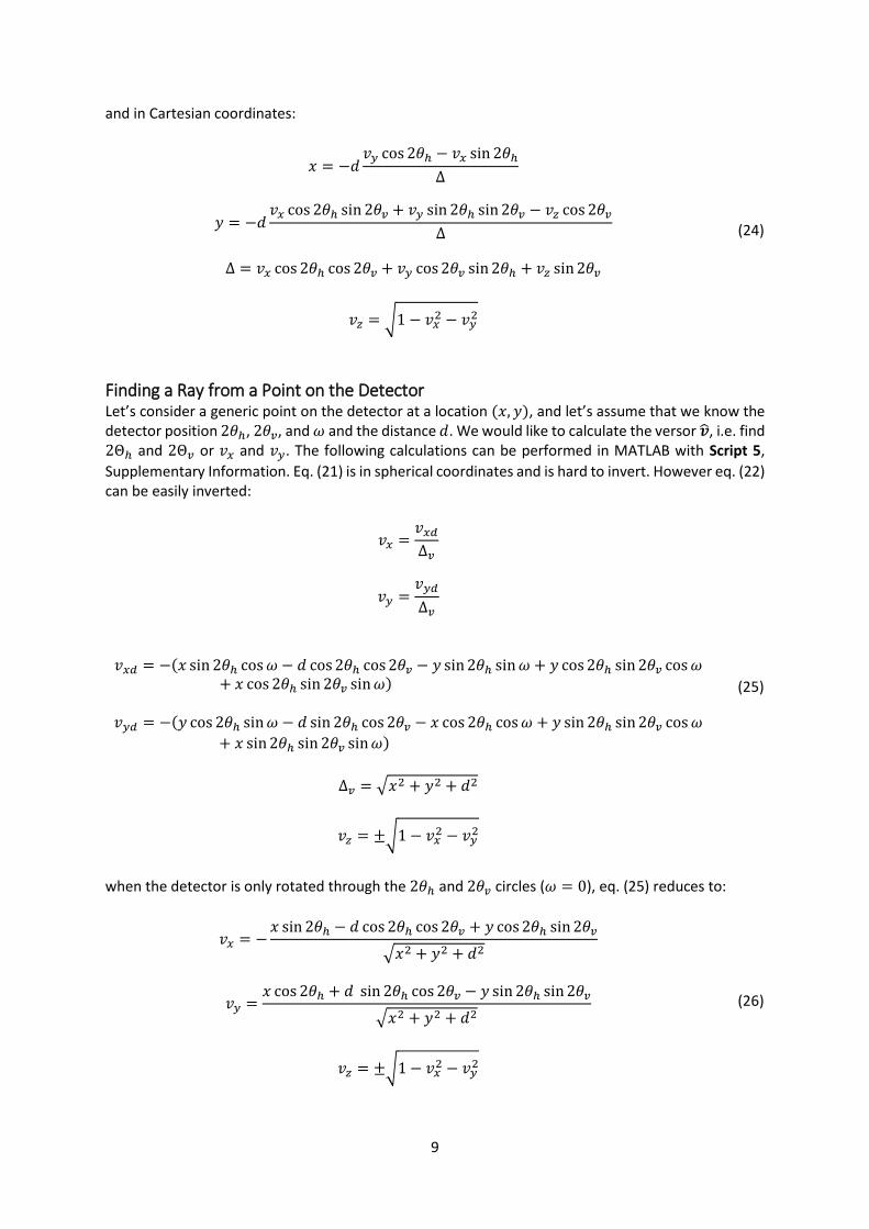
Finding a Ray from a Point on the Detector Let’s consider a generic point on the detector at a location (𝑥, 𝑦), and let’s assume that we know the detector position 2𝜃ℎ, 2𝜃𝑣, and 𝜔 and the distance 𝑑. We would like to calculate the versor �̂�, i.e. find 2Θℎ and 2Θ𝑣 or 𝑣𝑥 and 𝑣𝑦. The following calculations can be performed in MATLAB with Script 5,
Supplementary Information. Eq. (21) is in spherical coordinates and is hard to invert. However eq. (22) can be easily inverted:
𝑣𝑥 =𝑣𝑥𝑑Δ𝑣
𝑣𝑦 =𝑣𝑦𝑑
Δ𝑣
𝑣𝑥𝑑 = −(𝑥 sin 2𝜃ℎ cos𝜔 − 𝑑 cos2𝜃ℎ cos2𝜃𝑣 − 𝑦 sin2𝜃ℎ sin𝜔 + 𝑦 cos2𝜃ℎ sin2𝜃𝑣 cos𝜔+ 𝑥 cos 2𝜃ℎ sin 2𝜃𝑣 sin𝜔)
𝑣𝑦𝑑 = −(𝑦 cos 2𝜃ℎ sin𝜔 − 𝑑 sin 2𝜃ℎ cos 2𝜃𝑣 − 𝑥 cos 2𝜃ℎ cos𝜔 + 𝑦 sin 2𝜃ℎ sin2𝜃𝑣 cos𝜔
+ 𝑥 sin2𝜃ℎ sin 2𝜃𝑣 sin𝜔)
Δ𝑣 = √𝑥2 + 𝑦2 + 𝑑2
𝑣𝑧 = ±√1− 𝑣𝑥2 − 𝑣𝑦
2
(25)
when the detector is only rotated through the 2𝜃ℎ and 2𝜃𝑣 circles (𝜔 = 0), eq. (25) reduces to:
𝑣𝑥 = −𝑥 sin 2𝜃ℎ − 𝑑 cos 2𝜃ℎ cos 2𝜃𝑣 + 𝑦 cos2𝜃ℎ sin2𝜃𝑣
√𝑥2 + 𝑦2 + 𝑑2
𝑣𝑦 =𝑥 cos 2𝜃ℎ + 𝑑 sin 2𝜃ℎ cos 2𝜃𝑣 − 𝑦 sin 2𝜃ℎ sin2𝜃𝑣
√𝑥2 + 𝑦2 + 𝑑2
𝑣𝑧 = ±√1− 𝑣𝑥2 − 𝑣𝑦
2
(26)
10
The versor �̂� can be then converted into spherical coordinates with conversion formulae from Cartesian to spherical coordinates:
2Θℎ = atan𝑣𝑦
𝑣𝑥
2Θ𝑣 = atan𝑣𝑧
√𝑣𝑥2 + 𝑣𝑦
2
(27)
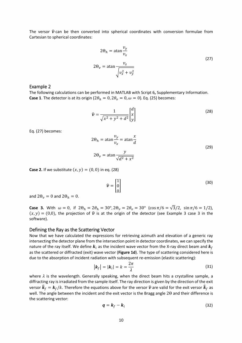
Example 2 The following calculations can be performed in MATLAB with Script 6, Supplementary Information. Case 1. The detector is at its origin (2𝜃ℎ = 0, 2𝜃𝑣 = 0,𝜔 = 0). Eq. (25) becomes:
�̂� =1
√𝑥2 + 𝑦2 + 𝑑2[𝑑𝑥𝑦]
(28)
Eq. (27) becomes:
2Θℎ = atan𝑣𝑦
𝑣𝑥= atan
𝑥
𝑑
2Θ𝑣 = atan𝑦
√𝑑2 + 𝑥2
(29)
Case 2. If we substitute (𝑥, 𝑦) = (0, 0) in eq. (28)
�̂� = [100]
(30)
and 2Θ𝑣 = 0 and 2Θℎ = 0.
Case 3. With 𝜔 = 0, if 2Θℎ = 2𝜃ℎ = 30°, 2Θ𝑣 = 2𝜃𝑣 = 30° (cos𝜋/6 = √3/2, sin𝜋/6 = 1/2), (𝑥, 𝑦) = (0,0), the projection of �̂� is at the origin of the detector (see Example 3 case 3 in the software).
Defining the Ray as the Scattering Vector Now that we have calculated the expressions for retrieving azimuth and elevation of a generic ray intersecting the detector plane from the intersection point in detector coordinates, we can specify the nature of the ray itself. We define 𝒌𝑖 as the incident wave vector from the X-ray direct beam and 𝒌𝑓
as the scattered or diffracted (exit) wave vector (Figure 1d). The type of scattering considered here is due to the absorption of incident radiation with subsequent re-emission (elastic scattering):
|𝒌𝑓| = |𝒌𝑖| = 𝑘 =2𝜋
𝜆 (31)
where 𝜆 is the wavelength. Generally speaking, when the direct beam hits a crystalline sample, a diffracting ray is irradiated from the sample itself. The ray direction is given by the direction of the exit
versor �̂�𝑓 = 𝒌𝑓/𝑘. Therefore the equations above for the versor �̂� are valid for the exit versor �̂�𝑓 as
well. The angle between the incident and the exit vector is the Bragg angle 2Θ and their difference is the scattering vector:
𝒒 = 𝒌𝑓 − 𝒌𝑖 (32)

11
The exit wave vector describes a sphere of radius 2𝜋/𝜆 called the Ewald sphere. More details on X-ray diffraction can be found elsewhere 1,4,38,39.
When the sample circles are zero the exit wave vector in laboratory coordinates is simply (see eq. (12) and eq. (15)):
𝒌𝑓 = 𝑘�̂�𝑓 = 𝑘 [
cos 2Θ𝑣 cos2Θℎcos 2Θ𝑣 sin2Θℎ
sin 2Θ𝑣
] = 𝑘 [
𝑘𝑓𝑥𝑘𝑓𝑦𝑘𝑓𝑧
] (33)
As discussed above the incident wave vector in laboratory coordinates30 points towards the �̂�𝑥 axis:
𝒌𝑖 = 𝑘�̂�𝑖 = 𝑘 [100] (34)
therefore the scattering vector in laboratory coordinates30 is:
𝒒 = 𝒌𝑓 − 𝒌𝑖 = 𝑘 [
cos 2Θ𝑣 cos2Θℎ − 1cos 2Θ𝑣 sin2Θℎ
sin2Θ𝑣
] = 𝑘 [𝑣𝑥 − 1𝑣𝑦𝑣𝑧
] (35)
The angle between the incident and exit vector is:
2Θ = ∠𝒌𝑓 , 𝒌𝑖 = acos𝒌𝑓 ∙ 𝒌𝑖
𝑘2= acos(cos 2Θℎ cos2Θ𝑣) (36)
The norm of 𝒒 is (using eq. (35) and the trigonometric relation 2 − 2 cos 2Θℎ = 4 sin
2 Θℎ):
|𝒒| = √(cos 2Θ𝑣 cos 2Θℎ − 1)2 + (cos 2Θ𝑣 sin2Θℎ)
2 + sin2 2Θ𝑣
= 𝑘√2 − 2 cos2Θ𝑣 cos 2Θℎ =4𝜋
𝜆sinΘ
(37)
In the case of 2Θ𝑣 = 0, |𝒒| =2𝜋
𝜆√2 − 2 cos 2Θℎ =
2𝜋
𝜆√4 sin2 Θℎ =
4𝜋
𝜆sinΘ.
Following You’s30 formalism we indicate the momentum transfer in the reciprocal space coordinates as:
𝒉 = ℎ𝒃1 + 𝑘𝒃2 + 𝑙𝒃3 (38)
where 𝒃1, 𝒃2, 𝒃3 are the reciprocal lattice vectors: 1,4,38,39
{
𝒃1 = 2𝜋
𝒂2 × 𝒂3 𝒂1 ∙ ( 𝒂2 × 𝒂3)
𝒃2 = 2𝜋 𝒂3 × 𝒂1
𝒂2 ∙ ( 𝒂3 × 𝒂1)
𝒃3 = 2𝜋 𝒂1 × 𝒂2
𝒂3 ∙ ( 𝒂1 × 𝒂2)
(39)
where 𝒂1, 𝒂2, 𝒂3 are the direct lattice vectors.
12
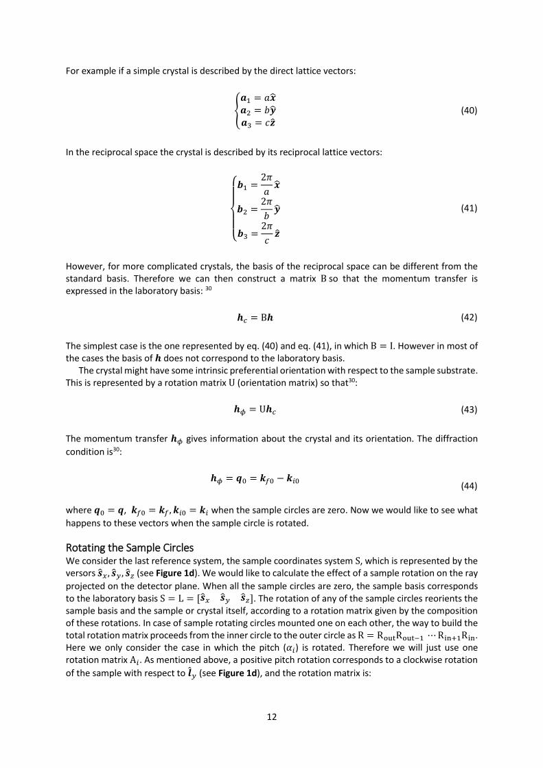
For example if a simple crystal is described by the direct lattice vectors:
{
𝒂1 = 𝑎�̂�𝒂2 = 𝑏�̂�𝒂3 = 𝑐�̂�
(40)
In the reciprocal space the crystal is described by its reciprocal lattice vectors:
{
𝒃1 =
2𝜋
𝑎�̂�
𝒃2 =2𝜋
𝑏�̂�
𝒃3 =2𝜋
𝑐�̂�
(41)
However, for more complicated crystals, the basis of the reciprocal space can be different from the standard basis. Therefore we can then construct a matrix B so that the momentum transfer is expressed in the laboratory basis: 30
𝒉𝑐 = B𝒉 (42)
The simplest case is the one represented by eq. (40) and eq. (41), in which B = I. However in most of the cases the basis of 𝒉 does not correspond to the laboratory basis.
The crystal might have some intrinsic preferential orientation with respect to the sample substrate. This is represented by a rotation matrix U (orientation matrix) so that30:
𝒉𝜙 = U𝒉𝑐 (43)
The momentum transfer 𝒉𝜙 gives information about the crystal and its orientation. The diffraction
condition is30:
𝒉𝜙 = 𝒒0 = 𝒌𝑓0 − 𝒌𝑖0
(44)
where 𝒒0 = 𝒒, 𝒌𝑓0 = 𝒌𝑓 , 𝒌𝑖0 = 𝒌𝑖 when the sample circles are zero. Now we would like to see what
happens to these vectors when the sample circle is rotated.
Rotating the Sample Circles We consider the last reference system, the sample coordinates system S, which is represented by the versors �̂�𝑥 , �̂�𝑦, �̂�𝑧 (see Figure 1d). We would like to calculate the effect of a sample rotation on the ray
projected on the detector plane. When all the sample circles are zero, the sample basis corresponds to the laboratory basis S = L = [�̂�𝑥 �̂�𝑦 �̂�𝑧]. The rotation of any of the sample circles reorients the sample basis and the sample or crystal itself, according to a rotation matrix given by the composition of these rotations. In case of sample rotating circles mounted one on each other, the way to build the total rotation matrix proceeds from the inner circle to the outer circle as R = RoutRout−1 ⋯Rin+1Rin. Here we only consider the case in which the pitch (𝛼𝑖) is rotated. Therefore we will just use one rotation matrix A𝑖. As mentioned above, a positive pitch rotation corresponds to a clockwise rotation
of the sample with respect to �̂�𝑦 (see Figure 1d), and the rotation matrix is:

13
Α𝑖 = [
cos𝛼𝑖 0 − sin𝛼𝑖0 1 0
sin𝛼𝑖 0 cos𝛼𝑖
] (45)
A pitch rotation, changes the sample basis from S = L = I, where all the sample circles are zero, to:
S′ = Α𝑖L = Α𝑖I = [cos 𝛼𝑖 0 − sin𝛼𝑖0 1 0
sin𝛼𝑖 0 cos𝛼𝑖
] (46)
Therefore in this simple case, the total rotation matrix is simply R = Α𝑖. In the presence of such a rotation the momentum transfer rotates according to30:
𝒉R = Α𝑖𝒉𝜙 (47)
The diffraction condition is30:
𝒉R = 𝒒 = 𝒌𝑓 − 𝒌𝑖
𝒒 = A𝑖𝒒0
𝒌𝑓 = A𝑖𝒌𝑓0
𝒌𝑖 = A𝑖𝒌𝑖0
(48)
This can be visualized in Figure 3, where 𝒌𝑓 and 𝒌𝑖 are the wave vectors in the laboratory reference
system (Figure 3a), while 𝒌𝑓0 and 𝒌𝑖0 are the wave vectors in the sample reference system (Figure
3a). The matrix A𝑖−1 = AT rotates the wave vectors 𝒌𝑓 and 𝒌𝑖 counterclockwise about �̂�𝑦, and allows
to express them as 𝒌𝑓0 and 𝒌𝑖0 in sample coordinates �̂�𝑥 , �̂�𝑦, �̂�𝑧.
Figure 3 – wave vectors in the laboratory (a) and sample (b) reference system.
Therefore the incident wave vectors in the laboratory and sample reference system are (see ref. 30 equation (12), where 𝐐𝐿 is our 𝒒):
𝒌𝑖 = 𝑘 [100]
𝒌𝑖0 = A𝑖−1𝒌𝑖 = 𝑘 [
cos𝛼𝑖0
− sin𝛼]
(49)

14
The exit wave vectors in the laboratory and sample basis are:
𝒌𝑓 = 𝑘 [
cos 2Θ𝑣 cos 2Θℎcos 2Θ𝑣 sin 2Θℎ
sin 2Θ𝑣
]
𝒌𝑓0 = A𝑖−1𝒌𝑓 = 𝑘 [
cos 2Θ𝑣0 cos2Θℎ0cos 2Θ𝑣0 sin2Θℎ0
sin2Θ𝑣0
]
(50)
The rotated scattering vector in the laboratory and sample reference system are:
𝒒 = 𝒉R = 𝒌𝑓 − 𝒌𝑖 = 𝑘 [
cos 2Θ𝑣 cos 2Θℎ − 1cos 2Θ𝑣 sin 2Θℎ
sin2Θ𝑣
]
𝒒0 = 𝒉𝜙 = 𝒌𝑓0 − 𝒌𝑖0 = 𝑘 [
cos 2Θ𝑣0 cos2Θℎ0 − cos𝛼𝑖cos 2Θ𝑣 sin 2Θℎsin 2Θ𝑣 + sin𝛼𝑖
]
(51)
Note that, obviously, 2Θ𝑣, 2Θℎ and 2Θ𝑣0, 2Θℎ0 are different and that 2Θ𝑣0, 2Θℎ0 are functions of 𝛼𝑖.
If we convert the detector coordinates from pixels to 𝒒0 we will be able to observe the reflection 𝒉𝜙 at the same point on the detector as 𝛼𝑖 varies. This is the most important concept of this
paragraph. If we exclude refraction effects40, by employing 𝒒0 as the image coordinates we can remove distortion effects in the diffraction pattern introduced by a non-zero pitch.
Reciprocal Space Mapping Equations As mentioned above, eq. (25)-(27) for a generic versor �̂�, can be used for the calculation of �̂�𝑓(= �̂�) in
the laboratory reference system:
𝑘𝑓𝑥 =𝑘𝑓𝑥𝑑
Δ𝑘
𝑘𝑓𝑦 =𝑘𝑓𝑦𝑑
Δ𝑘
𝑘𝑓𝑥𝑑 = −(𝑥 sin 2𝜃ℎ cos𝜔 − 𝑑 cos2𝜃ℎ cos2𝜃𝑣 − 𝑦 sin2𝜃ℎ sin𝜔 + 𝑦 cos2𝜃ℎ sin2𝜃𝑣 cos𝜔
+ 𝑥 cos 2𝜃ℎ sin 2𝜃𝑣 sin𝜔)
𝑘𝑓𝑦𝑑 = −(𝑦 cos 2𝜃ℎ sin𝜔 − 𝑑 sin 2𝜃ℎ cos 2𝜃𝑣 − 𝑥 cos 2𝜃ℎ cos𝜔 + 𝑦 sin 2𝜃ℎ sin2𝜃𝑣 cos𝜔
+ 𝑥 sin2𝜃ℎ sin 2𝜃𝑣 sin𝜔)
𝑘𝑓𝑧 = √1 − 𝑘𝑓𝑥2 − 𝑘𝑓𝑦
2
Δ𝑘 = √𝑥2 + 𝑦2 + 𝑑2
2Θℎ = atan𝑘𝑓𝑦
𝑘𝑓𝑥
(52)

15
2Θ𝑣 = atan𝑘𝑓𝑧
√𝑘𝑓𝑥2 + 𝑘𝑓𝑦
2
If the sample circles have been rotated, the exit wave versor in the sample reference system is (see eq. (50)):
�̂�𝑓0 = A𝑖−1�̂�𝑓 = [
cos𝛼𝑖 0 sin𝛼𝑖0 1 0
− sin𝛼𝑖 0 cos𝛼𝑖
] [
𝑘𝑓𝑥𝑘𝑓𝑦𝑘𝑓𝑧
] (53)
The exit wave versor azimuth and elevation are:
2Θℎ0 = atan𝑘𝑓𝑦0
𝑘𝑓𝑥0
2Θ𝑣0 = atan𝑘𝑓𝑧0
√𝑘𝑓𝑥02 + 𝑘𝑓𝑦0
2
(54)
Once �̂�𝑓0has been calculated, the scattering vector (or momentum transfer) in the sample reference
system can be easily extracted:
𝒉𝜙 = 𝒒0 = [
𝑞𝑥0𝑞𝑦0𝑞𝑧0
] = 𝑘 [
𝑘𝑓𝑥0 − cos𝛼𝑖𝑘𝑓𝑦0
𝑘𝑓𝑧0 + sin𝛼𝑖
] = 𝑘 [
cos 2Θ𝑣0 cos 2Θℎ0 − cos𝛼𝑖cos 2Θ𝑣0 sin2Θℎ0sin2Θ𝑣0 + sin𝛼𝑖
] (55)
Note that eq. (55) is equivalent to the relations mapping the image of the untilted fibre from the detector plane into reciprocal space, which is reported in ref. 41. Finally, the reciprocal space mapping conversion procedure can be summarized as follows:
1) Define (𝑥, 𝑦) pixel reference system for the diffraction image. There might be cases in which, when the detector and sample circle angles are zero, the direct beam is not at the centre of the detector. In this case the origin of the image (𝑥0, 𝑦0) cannot be at the centre of the diffraction pattern, and has to be set to the point where the direct beam hits the detector (eq. (16));
2) Extract image pixel coordinates (𝑥, 𝑦) from the diffraction image and retrieve 2𝜃ℎ, 2𝜃𝑣, 𝜔 and 𝑑. If the detector is mounted on the detector circles the distance 𝑑 can be calculated by tracking the direct beam, as shown in ref.40. The angles 2𝜃ℎ, 2𝜃𝑣, 𝜔 are immediately available if the detector is mounted on the detector circles. However there can be cases in which the detector is mounted elsewhere (e.g. linear stages). In this case a calibration material (e.g. silver behenate) can be used for the extraction of 2𝜃ℎ, 2𝜃𝑣, and 𝑑.
3) Use eq. (52) to convert (𝑥, 𝑦) to �̂�𝑓;
4) Use eq. (53) to obtain the exit wave versor �̂�𝑓0 from �̂�𝑓;
5) Use eq. (55) to calculate the momentum transfer or scattering vector 𝒒0 in the sample reference system;
6) Remap the intensities (interpolation) from the original diffraction image in (𝑥, 𝑦) coordinates
into suitable 2D coordinates for 𝒒0, for example 𝑞𝑧0 as the ordinate and 𝑞𝑥𝑦0 = √𝑞𝑥02 + 𝑞𝑦0
2
as the abscissa.

16
Conclusion In this work we have derived, in a rigorous way, the reciprocal space mapping equations for a ‘3D+1S’ diffractometer in a way that is understandable to anyone with basic notions of linear algebra, geometry, and X-ray diffraction. With this set of equations, starting from the detector and sample circle angles and the distance sample-detector one can convert a diffraction image represented in pixel coordinates to the momentum transfer or scattering vector in the sample reference system.
References 1 Birkholz, M. Thin film analysis by X-ray scattering. (John Wiley & Sons, 2006). 2 Vlieg, E., Van der Veen, J., Macdonald, J. & Miller, M. Angle calculations for a five-circle
diffractometer used for surface X-ray diffraction. Journal of applied crystallography 20, 330-337, (1987).
3 Feidenhans, R. Surface structure determination by X-ray diffraction. Surface Science Reports 10, 105-188, (1989).
4 Als-Nielsen, J. & McMorrow, D. Elements of modern X-ray physics. (John Wiley & Sons, 2011). 5 Ungar, G., Liu, F., Zeng, X., Glettner, B., Prehm, M., Kieffer, R. et al. in Journal of Physics:
Conference Series. 012032 (IOP Publishing). 6 Grelet, E., Dardel, S., Bock, H., Goldmann, M., Lacaze, E. & Nallet, F. Morphology of open films
of discotic hexagonal columnar liquid crystals as probed by grazing incidence X-ray diffraction. The European Physical Journal E 31, 343-349, (2010).
7 Perlich, J., Schwartzkopf, M., Körstgens, V., Erb, D., Risch, J., Müller‐Buschbaum, P. et al. Pattern formation of colloidal suspensions by dip‐coating: An in situ grazing incidence X‐ray scattering study. Physica status solidi (RRL)-Rapid Research Letters 6, 253-255, (2012).
8 Renaud, G., Lazzari, R. & Leroy, F. Probing surface and interface morphology with Grazing Incidence Small Angle X-Ray Scattering. Surface Science Reports 64, 255-380, (2009).
9 Bikondoa, O., Carbone, D., Chamard, V. & Metzger, T. H. Ageing dynamics of ion bombardment induced self-organization processes. Scientific Reports 3, 1850, (2013).
10 Joshi, G. R., Cooper, K., Lapinski, J., Engelberg, D. L., Bikondoa, O., Dowsett, M. G. et al. (NACE International).
11 Springell, R., Rennie, S., Costelle, L., Darnbrough, J., Stitt, C., Cocklin, E. et al. Water corrosion of spent nuclear fuel: radiolysis driven dissolution at the UO2/water interface. Faraday Discussions 180, 301-311, (2015).
12 Katsouras, I., Asadi, K., Li, M., van Driel, T. B., Kjaer, K. S., Zhao, D. et al. The negative piezoelectric effect of the ferroelectric polymer poly(vinylidene fluoride). Nat Mater, (2015).
13 Müller-Buschbaum, P. Grazing incidence small-angle X-ray scattering: an advanced scattering technique for the investigation of nanostructured polymer films. Anal Bioanal Chem 376, 3-10, (2003).
14 Dane, T. G., Cresswell, P. T., Pilkington, G. A., Lilliu, S., Macdonald, J. E., Prescott, S. W. et al. Oligo(aniline) nanofilms: from molecular architecture to microstructure. Soft Matter 9, 10501-10511, (2013).
15 Al-Jawad, M., Steuwer, A., Kilcoyne, S. H., Shore, R. C., Cywinski, R. & Wood, D. J. 2D mapping of texture and lattice parameters of dental enamel. Biomaterials 28, 2908-2914, (2007).
16 Simmons, L. M., Al‐Jawad, M., Kilcoyne, S. H. & Wood, D. J. Distribution of enamel crystallite orientation through an entire tooth crown studied using synchrotron X‐ray diffraction. European journal of oral sciences 119, 19-24, (2011).
17 Beddoes, C. M., Case, C. P. & Briscoe, W. H. Understanding nanoparticle cellular entry: A physicochemical perspective. Advances in Colloid and Interface Science 218, 48-68, (2015).
18 Renaud, G. Oxide surfaces and metal/oxide interfaces studied by grazing incidence X-ray scattering. Surface Science Reports 32, 5-90, (1998).
17
19 Staniec, P. A., Parnell, A. J., Dunbar, A. D., Yi, H., Pearson, A. J., Wang, T. et al. The nanoscale morphology of a PCDTBT: PCBM photovoltaic blend. Advanced Energy Materials 1, 499-504, (2011).
20 Agostinelli, T., Ferenczi, T. A., Pires, E., Foster, S., Maurano, A., Müller, C. et al. The role of alkane dithiols in controlling polymer crystallization in small band gap polymer: Fullerene solar cells. Journal of Polymer Science Part B: Polymer Physics 49, 717-724, (2011).
21 Lilliu, S., Agostinelli, T., Hampton, M., Pires, E., Nelson, J. & Macdonald, J. E. The Influence of Substrate and Top Electrode on the Crystallization Dynamics of P3HT: PCBM Blends. Energy Procedia 31, 60-68, (2012).
22 Lilliu, S., Alsari, M., Bikondoa, O., Macdonald, J. E. & Dahlem, M. S. Absence of Structural Impact of Noble Nanoparticles on P3HT:PCBM Blends for Plasmon-Enhanced Bulk-Heterojunction Organic Solar Cells Probed by Synchrotron GI-XRD. Scientific Reports, (2015).
23 Juraić, K., Gracin, D., Šantić, B., Meljanac, D., Zorić, N., Gajović, A. et al. GISAXS and GIWAXS analysis of amorphous–nanocrystalline silicon thin films. Nuclear Instruments and Methods in Physics Research Section B: Beam Interactions with Materials and Atoms 268, 259-262, (2010).
24 Treat, N. D., Brady, M. A., Smith, G., Toney, M. F., Kramer, E. J., Hawker, C. J. et al. Interdiffusion of PCBM and P3HT reveals miscibility in a photovoltaically active blend. Advanced Energy Materials 1, 82-89, (2011).
25 Rogers, J. T., Schmidt, K., Toney, M. F., Kramer, E. J. & Bazan, G. C. Structural order in bulk heterojunction films prepared with solvent additives. Advanced Materials 23, 2284-2288, (2011).
26 Büchele, P., Richter, M., Tedde, S. F., Matt, G. J., Ankah, G. N., Fischer, R. et al. X-ray imaging with scintillator-sensitized hybrid organic photodetectors. Nature Photonics, (2015).
27 Tsao, H. N., Cho, D., Andreasen, J. W., Rouhanipour, A., Breiby, D. W., Pisula, W. et al. The Influence of Morphology on High‐Performance Polymer Field‐Effect Transistors. Advanced Materials 21, 209-212, (2009).
28 Nelson, T. L., Young, T. M., Liu, J., Mishra, S. P., Belot, J. A., Balliet, C. L. et al. Transistor paint: high mobilities in small bandgap polymer semiconductor based on the strong acceptor, diketopyrrolopyrrole and strong donor, dithienopyrrole. Advanced Materials 22, 4617-4621, (2010).
29 He, B. B. Two-dimensional X-ray diffraction. (John Wiley & Sons, 2011). 30 You, H. Angle calculations for a `4S+2D' six-circle diffractometer. Journal of Applied
Crystallography 32, 614-623, (1999). 31 Banchoff, T. & Wermer, J. Linear algebra through geometry. (Springer Science & Business
Media, 2012). 32 Bloom, D. M. Linear algebra and geometry. (CUP Archive, 1979). 33 Kostrikin, A. I., Manin, Y. I. & Alferieff, M. E. Linear algebra and geometry. (Gordon and Breach
Science Publishers, 1997). 34 Shafarevich, I. R. & Remizov, A. Linear algebra and geometry. (Springer Science & Business
Media, 2012). 35 Hase, T. Beamline Description,
<http://www2.warwick.ac.uk/fac/cross_fac/xmas/description/> (2015). 36 Boesecke, P. Reduction of two-dimensional small-and wide-angle X-ray scattering data.
Applied Crystallography, (2007). 37 Murray, G. Rotation About an Arbitrary Axis in 3 Dimensions,
<http://inside.mines.edu/fs_home/gmurray/ArbitraryAxisRotation/> (2013). 38 Woolfson, M. M. An introduction to X-ray crystallography. (Cambridge University Press,
1997). 39 Warren, B. E. X-ray Diffraction. (Courier Corporation, 1969).

18
40 Lilliu, S., Agostinelli, T., Pires, E., Hampton, M., Nelson, J. & Macdonald, J. E. Dynamics of crystallization and disorder during annealing of P3HT/PCBM bulk heterojunctions. Macromolecules 44, 2725-2734, (2011).
41 Stribeck, N. & Nöchel, U. Direct mapping of fiber diffraction patterns into reciprocal space. Journal of Applied Crystallography 42, 295-301, (2009).
42 Ohad, G. fit_ellipse, <http://www.mathworks.com/matlabcentral/fileexchange/3215-fit-ellipse> (2003).

19
Supplementary Information The following table summarizes typical values encountered in grazing incidence wide (WAXS) and small (SAXS) angle scattering.
Table 1 – Typical values.
Symbol Description Typical values
𝑝 pixel size (e.g. MAR) 80 [µm/pixel]
𝑑 distance sample detector in WAXS 20mm, 2.5×103 pixel
𝑑 distance sample detector in SAXS 10m, 125×103 pixel
2𝜃ℎ detector circle angle (azimuth) -10, 10 [°]
2𝜃𝑣 detector circle angle (elevation) -10, 10 [°]
𝜔 detector circle angle (rotation) 0 [°]
𝛼𝑖 sample circle angle (pitch) 0, 0.5 [°]
𝜆 wavelength 1.23984 [Å]
Detector-GUI Matlab A simple software (detector-GUI Matlab) has been developed to illustrate the examples above and can be downloaded from this link1. This is how the GUI looks like when it is launched. Note that the remapping equations do not take into account 𝜔 rotation (therefore 𝜔 should be always set to zero). The input fields are highlighted in green.
Figure 4 - detector-GUI Matlab software.
We can start by loading Example 1 from the popup menu ‘Load Example’. The parameters used in Example 1 are automatically loaded into the GUI. The following parameters can be inserted in the panel below: 𝑑 (distance in pixels), detector width and height (in pixels), detector circle angles (azimuth 2𝜃ℎ, elevation 2𝜃ℎ, and omega 𝜔), sample pitch (𝛼𝑖).
1 https://www.dropbox.com/sh/5x9ff444f5iybdj/AACwQTm3tq8dqF3eM7FdGnYsa?dl=0

20
After entering any value, pressing Enter updates the calculations and the display items in the figures.
The first four figures depict a red rectangle representing the edges of a square detector, while the black line represents the normal to the detector. The fifth figure depicts the incident wave vector and the sample edge at a specific 𝛼𝑖. The sixth figure shows the projected ray on the detector in detector coordinates. The seventh figure shows the same point in 𝑞𝑧0 and 𝑞𝑥𝑦0 coordinates. The eighth figure
shows the same point in 𝑞𝑧 and 𝑞𝑥𝑦 coordinates.
In the following panel you can control the direct beam and the beam energy or wavelength (𝜆). Note that when an energy value is entered wavelength and 2pi/wav (2𝜋/𝜆) are automatically updated.
With the following panel you can control the exit wave vector azimuth (2Θℎ) and elevation (2Θ𝑣). Equivalently you can enter a lattice constant value 𝑐 (cubic crystal). The software calculates the elevation corresponding to the lattice value using the Bragg’s law.
The 𝒒0 and 𝒌𝑓0 vectors are automatically calculated.

21
The 𝒒, 𝒌𝑓, and 𝒌𝑖 vectors are also calculated (obviously if 𝛼𝑖 = 0, 𝒒 = 𝒒0 and 𝒌𝑓0 = 𝒌𝑓).
The blue point displayed in figure six is calculated with eq. (23). The values in the following panel are calculated with eq. (55) from the (𝑥, 𝑦) coordinates of the point displayed in figure six.
The following parameters are just for tests and should be discarded42.

22
Symbolic Calculations The following scripts are independent from the detector-GUI Matlab software and require the Symbolic Math Toolbox.
Script 1 – Arbitrary matrix rotation constructor. This function is used in the following scripts.
function R = arb_rot_sim(a,vect)
% Rotation about arbitrary axis for symb calculations
%vect = vect / norm (vect);
u = vect(1); v = vect(2); w = vect(3);
u2 = u^2 ; v2 = v^2 ; w2 = w^2;
c = cos(a); s = sin(a);
R(1,1) = u2 + (1-u2)*c;
R(1,2) = u*v*(1-c) - w*s;
R(1,3) = u*w*(1-c) + v*s;
R(2,1) = u*v*(1-c) + w*s;
R(2,2) = v2 + (1-v2)*c;
R(2,3) = v*w*(1-c) - u*s;
R(3,1) = u*w*(1-c) - v*s;
R(3,2) = v*w*(1-c)+u*s;
R(3,3) = w2 + (1-w2)*c;
Script 2 – Calculates rotation matrices. See Tracking the Detector Movement.
%% Tracking the Detector Movement
clear all
syms h2 v2 om real % detector rotation angles (azimuth, elevation, omega)
Rx = arb_rot_sim(om,[1 0 0]') % eq.(2)
Ry = arb_rot_sim(v2,-[0 1 0]') % eq.(3)
Rz = arb_rot_sim(h2,[0 0 1]') % eq.(4)
Rxyz = simplify(Rz*Ry*Rx) % eq.(5), total rot. matrix
isequal(simplify(Rxyz'), simplify(Rxyz^-1)) % matrix orthogonality check
isequal(simplify(det(Rxyz)),1) % det = 1 check
Ryz = simplify(Rz*Ry) % eq.(7), total rot. matrix with om = 0
Script 3 – Projecting a ray onto the detector. Running Script 2 is required before running this script. See Projecting a Ray onto the Detector.
%% Projecting a Ray onto the Detector
syms H2 V2 d real % ray azimuth and elevation, sample-dectector distance
syms vx vy vz real % ray Cartesian coordiantes
n = [1 0 0]' % eq.(9), normal versor to unrotated detector
[V(1) V(2) V(3)] = sph2cart(H2, V2, 1); V = V' % eq.(12), ray sph. coord
n2 = Rxyz*n % eq.(13), rotated versor
P = d*V/dot(V, n2) % eq.(14), intersection point with detector
Pnum = d*V % numerator in eq. (14)
Pden = dot(V, n2) % numerator in eq. (14)
Vxyz = [vx vy vz]' % eq.(15), ray Carthesian coordinates
P1 = d*Vxyz/dot(Vxyz, n2) % eq.(15), intersection point with detector
P1num = d*Vxyz % numerator in eq. (15)
P1den = dot(Vxyz, n2) % numerator in eq. (15)
Script 4 – Projecting a ray onto the detector. Running Script 3 is required before running this script.
%% Ray Projection on Detector Coordinate System
dy = [0 1 0 ]' % detector x axis
dz = [0 0 1 ]' % detector y axis
dx = [0 0 0 ]' % zero column, detector coord are in 2D
D = [dx , dy, dz] % eq.(18) detector basis
dy2 = Rxyz*dy % eq.(19) roatated detector x axis
dz2 = Rxyz*dz % eq.(19) rotated detector y axis
D2 = Rxyz*D % eq.(19) rotated detector coordinate system

23
x = simplify(dot(P, dy2)); % eq.(21), point P in detector coordiantes
y = simplify(dot(P, dz2)); % eq.(21), point P in detector coordiantes
x1 = simplify(dot(P1, dy2)); % eq.(22), point P in detector coordiantes
y1 = simplify(dot(P1, dz2)); % eq.(22), point P in detector coordiantes
x1 = simplify(subs(x1, vz, sqrt(1-vx^2-vy^2))) % eq.(22)
y1 = simplify(subs(y1, vz, sqrt(1-vx^2-vy^2))) % eq.(22)
simplify(subs(x1, om, 0)) % eq.(24)
simplify(subs(y1, om, 0)) % eq.(24) Script 5 – Projecting a ray onto the detector. Running Script 4 is required before running this script. See Finding a Ray from a Point on the Detector.
%% Finding a Ray from a Point on the Detector
syms X Y real
[vx_s vy_s] = solve([X == x1, Y == y1], vx, vy) % inverting eq.(22)
simplify(vx_s(2)) % eq.(25), vx (only the second solution makes sense)
simplify(vy_s(2)) % eq.(25), vy
vz_s = simplify(sqrt(1-vx_s(2)^2-vy_s(2)^2))
subs(simplify(vx_s(2)), om, 0) % eq.26, vx
subs(simplify(vy_s(2)), om, 0) % eq.26, vy
Script 6 – Example 2. Running script 5 is required before running this script. See Example .
%% Example 2
% case 1
subs(vx_s(2), [h2 v2 om], [0 0 0]) % eq.(40), vx
subs(vy_s(2), [h2 v2 om], [0 0 0]) % eq.(40), vy
simplify(subs(vz_s, [h2 v2 om], [0 0 0])) % eq.(4), vz
% case 3
c3x = double(subs(vx_s(2), [h2 v2 X Y d om], [pi/6 pi/6 0 0 1 0])) % eq.(43)
c3y = double(subs(vy_s(2), [h2 v2 X Y d om], [pi/6 pi/6 0 0 1 0])) % eq.(43)
c3z = double(simplify(subs(vz_s, [h2 v2 X Y d om], [pi/6 pi/6 0 0 1 0])))%
eq.(43)
c3 = [c3x c3y c3z];
[ca ce cr] = cart2sph(c3x, c3y, c3z);
ca_deg = rad2deg(ca) % eq.(44)
ce_deg = rad2deg(ce) % eq.(44)
Script 7 – Scattering Vector.
%% Defining the Ray as the Scattering Vector
syms lam real % wave vector amplitude 2pi/lambda
k = 2*pi/lam;
ki = [1 0 0]'
kf = V
q = kf-ki % eq.(35)
simplify(acos(dot(ki, kf))) % Bragg angle
simplify(sqrt(dot(q,q))) % eq. (37) norm of q0
syms a b c real
a1 = [a 0 0]
a2 = [0 b 0]
a3 = [0 0 c]
b1 = 2*pi*(cross(a2, a3)/dot(a1,(cross(a2, a3))))
b2 = 2*pi*(cross(a3, a1)/dot(a2,(cross(a3, a1))))
b3 = 2*pi*(cross(a1, a2)/dot(a3,(cross(a1, a2))))
Script 8 – Unrotated exit wave vector. Running script 6 is required before running this script.
%% Rotating the sample circles
syms ai real

24
kfx = simplify(vx_s(2)) % eq.25, vx
kfy = simplify(vy_s(2)) % eq.25, vy
kfz = simplify(sqrt(1-vx_s(2)^2-vy_s(2)^2))
kf = [kfx; kfy; kfz]
Ai = arb_rot_sim(ai,-[0 1 0]'); % eq.(45) pitch rotation matrix