Recent trends in the inverse problem of the...

Recent trends in the inverse problem of the calculus of variations

1

Beijing, July 2016

D. Krupka

Lepage Research Institute


Contents

Part I

The inverse problem of the calculus of variations: An outline

Part II

Applications

- variational completion of differential equations

- geometric mechanics

- homogeneous differential equations

- the Sonin-Douglas’s problem

- geometric control theory

- energy-momentum tensors

D. Krupka

2

Basic references

Variational calculus on fibred manifolds: General theory

D. Krupka, Introduction to Global Variational Geometry, Atlantis Studies

in Variational Geometry, Atlantis Press 2015, Book DOI: 10.2991/978-94-

6239-0737, 371 pp.

Specific topics

D.V. Zenkov, Editor, The Inverse Problem of the Calculus of Variations,

Local and Global Theory, Atlantis Press, 2015, 1-29

Chapters:

- A.M. Bloch, D. Krupka and D.V. Zenkov, The Helmholtz Conditions

and the Method of Controlled Lagrangians

- D. Krupka, The Sonin–Douglas Problem

- Z. Urban, Variational Principles for Immersed Submanifolds

- N. Voicu, Source Forms and Their Variational Completions


3

Part I

The inverse problem of the calculus of variations: An outline

Aim: to introduce basic concepts of variational theory on fibred mani-

folds on simple (classical) mathematical spaces: Euclidean spaces. All

concepts can be explained on general fibered manifolds and fibre bundles.

Euclidean spaces, canonical coordinates

Rn , x i , 1 £ i £ n

Rm , ys , 1 £ s £ m

Rn ´Rm , (x i , ys ),

Rn ´Rm ´Rnm , (x i , ys , y js ),

Rn ´Rm ´Rnm ´R1

2mn(n+1)

, (x i , ys , y js , y jk

s )

Differential equations

(1) en (xi ,ys ,y js ,y jk

s ) = 0

Aim: to study possibilities to construct a variational principle for (1)

D. Krupka

4

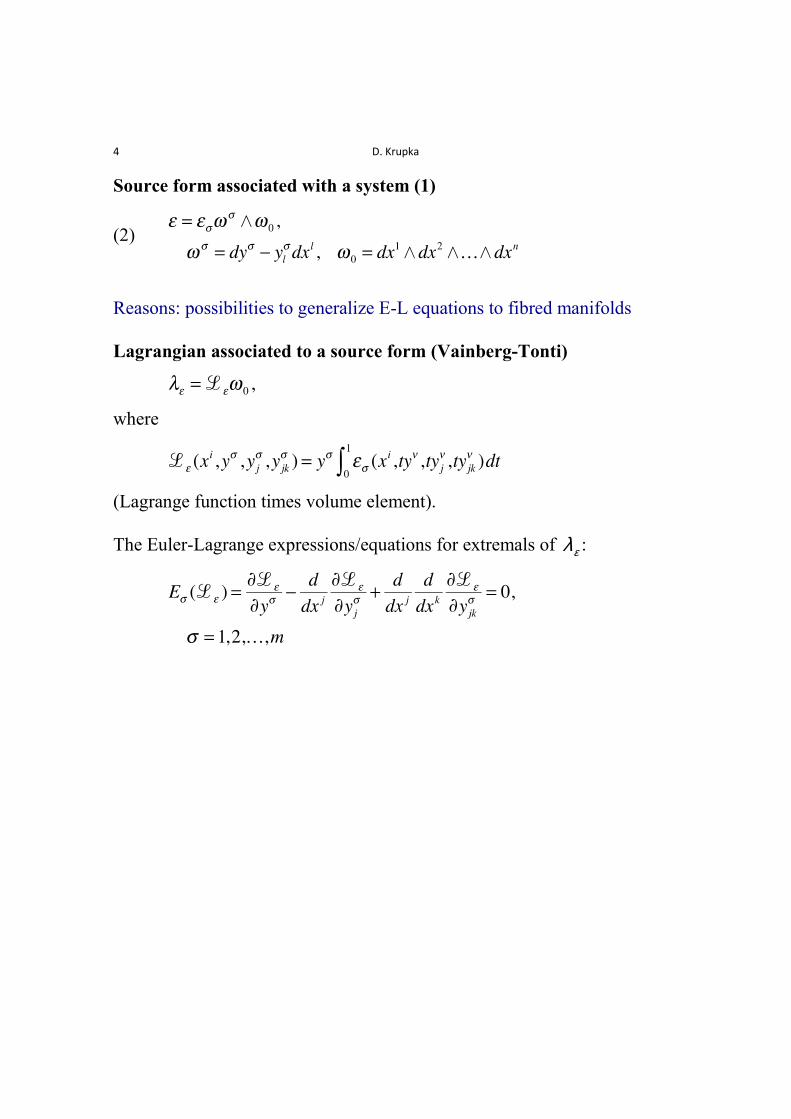
Source form associated with a system (1)

(2)

Reasons: possibilities to generalize E-L equations to fibred manifolds

Lagrangian associated to a source form (Vainberg-Tonti)

where

(Lagrange function times volume element).

The Euler-Lagrange expressions/equations for extremals of le:


5

Theorem The Euler-Lagrange expressions of the Vainberg-Tonti La-

grangian le of a source form are

(integration along segment) where

(3)

Hs n

ij (e ) =∂es

∂yijn

-∂en

∂yijs

,

Hs n

i (e ) =∂es

∂yin

+∂en

∂yis

- 2d j∂en

∂yijs

,

Hs n (e ) =∂es

∂yn-

∂en

∂ys+ di

∂en

∂yis

- did j∂en

∂yijs

.

The Helmholtz expressions, associated with the source form e .

The theorem describes the difference between the given equations and

the Euler-Lagrange equations of the Vainberg-Tonti Lagrangian; we see, in

particular, that responsibility for the difference is characterized by the

Helmholtz expressions.

D. Krupka

6

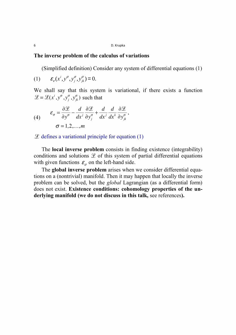
The inverse problem of the calculus of variations

(Simplified definition) Consider any system of differential equations (1)

(1) en (xi ,ys ,y js ,y jk

s ) = 0.

We shall say that this system is variational, if there exists a function

such that

(4)

defines a variational principle for equation (1)

The local inverse problem consists in finding existence (integrability)

conditions and solutions of this system of partial differential equations

with given functions es on the left-hand side.

The global inverse problem arises when we consider differential equa-

tions on a (nontrivial) manifold. Then it may happen that locally the inverse

problem can be solved, but the global Lagrangian (as a differential form)

does not exist. Existence conditions: cohomology properties of the un-

derlying manifold (we do not discuss in this talk, see references).


7

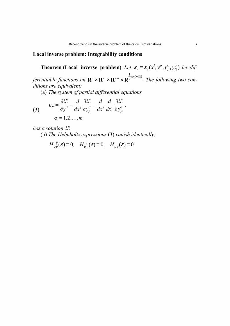
Local inverse problem: Integrability conditions

Theorem (Local inverse problem) Let en = en (xi ,ys ,y js ,y jk

s ) be dif-

ferentiable functions on Rn ´Rm ´Rnm ´R

1

2mn(n+1)

. The following two con-

ditions are equivalent:

(a) The system of partial differential equations

(3)

has a solution .

(b) The Helmholtz expressions (3) vanish identically,

Hs n

ij (e ) = 0, Hs n

i (e ) = 0, Hsn (e ) = 0.

D. Krupka

8

Remark (Sonin, Helmholtz, Douglas) The inverse problem of the

calculus of variations was first considered in 1886 for one second-order or-

dinary differential equation by Sonin. He proved that every second order

equation has a Lagrangian. It should be pointed out that in this paper the

variational multiplier, in contemporary terminology, was used as a natural

factor ensuring covariance of the considered equation. The variationality of

systems of second-order ordinary differential equations, expressed in the

covariant form, was studied by Helmholtz in 1887 and subsequently by

many followers (see e.g Havas). The systems of second-order ordinary dif-

ferential equations, solved with respect to the second derivatives, were con-

sidered by Douglas in 1940 with the techniques of variational multipliers

(see also Anderson and Thompson, Bucataru, Crampin, Sarlet, Crampin

and Martinez and many others).

Remark Global problem: Variational sequences (Krupka 1990).

Many contributors: Francaviglia, Ferraris, Winterroth, Palese, Vitolo,

Moreno (Italy); Grigore (Romania); Sardanashvily (Russia), Pommaret

(France), Krupka, Urban,Volna, Krbek, Musilova, (Czech Republic), etc.

Variational bicomplexes (Anderson (USA), Takens (Netherland),

Vinogradov (Russia), Saunders (GB), …


9

Part II

APPLICATIONS

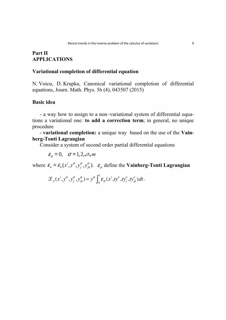
Variational completion of differential equation

N. Voicu, D. Krupka, Canonical variational completion of differential

equations, Journ. Math. Phys. 56 (4), 043507 (2015)

Basic idea

- a way how to assign to a non–variational system of differential equa-

tions a variational one: to add a correction term; in general, no unique

procedure

- variational completion: a unique way based on the use of the Vain-

berg-Tonti Lagrangian Consider a system of second order partial differential equations

es = 0, s =1,2,…,m

where en = en (xi ,ys ,y js ,y jk

s ). es define the Vainberg-Tonti Lagrangian

D. Krupka

10

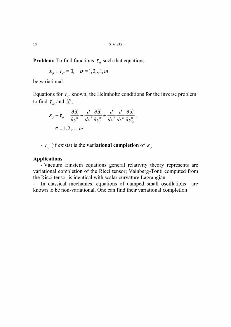
Problem: To find functions ts such that equations

es +ts = 0, s =1,2,…,m

be variational.

Equations for ts known; the Helmholtz conditions for the inverse problem

to find ts and ;

- ts (if exists) is the variational completion of es

Applications

- Vacuum Einstein equations general relativity theory represents are

variational completion of the Ricci tensor; Vainberg-Tonti computed from

the Ricci tensor is identical with scalar curvature Lagrangian

- In classical mechanics, equations of damped small oscillations are

known to be non-variational. One can find their variational completion


11

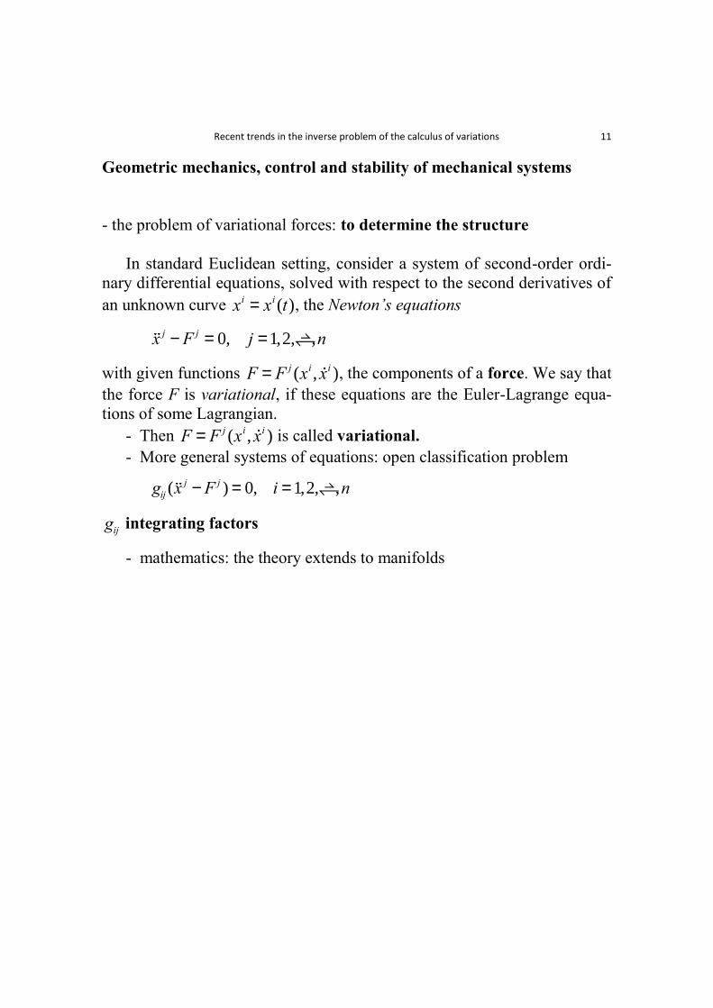
Geometric mechanics, control and stability of mechanical systems

- the problem of variational forces: to determine the structure

In standard Euclidean setting, consider a system of second-order ordi-

nary differential equations, solved with respect to the second derivatives of

an unknown curve xi = xi (t), the Newton’s equations

xj - F j = 0, j =1,2,…,n

with given functions F = F j (xi ,xi ), the components of a force. We say that

the force F is variational, if these equations are the Euler-Lagrange equa-

tions of some Lagrangian.

- Then F = F j (xi ,xi ) is called variational.

- More general systems of equations: open classification problem

gij (x

j - F j ) = 0, i = 1,2,…,n

gij integrating factors

- mathematics: the theory extends to manifolds

D. Krupka

12

Many results known, however, systematic exposition is needed.

References: W. Sarlet (Begium) and his school, Novotny, Krupkova,

Musilova and others (Czechia, Slovakia)

- control; to determine control parameters

A.M Bloch, D. Krupka and D.V. Zenkov, The Helmholtz Conditions

and the Method of Controlled Lagrangians, in The Inverse Prob-

lem of the Calculus of Variations, Local and Global Theory

Usual approach and methods: Methods applied: experimenal mathe-

matics based on modification of parameters in equations of motion (such

as force, energy)

Mathematical problem: given a system of equations describing the

motion of a mechanical system, introduce parameters into these equations

(e.g. by modifying the force, kinetic energy, geometric parameters like

constraints, …), and determine these parameters from the requirement

that the equations have a variational principle (Bloch, Krupka, Zenkov) tools: Helmholtz conditions


13

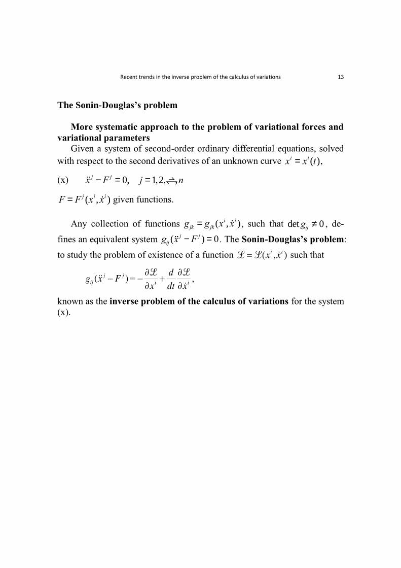
The Sonin-Douglas’s problem

More systematic approach to the problem of variational forces and

variational parameters

Given a system of second-order ordinary differential equations, solved

with respect to the second derivatives of an unknown curve xi = xi (t),

(x) xj - F j = 0, j =1,2,…,n

F = F j (xi ,xi ) given functions.

Any collection of functions g jk = g jk (x

i ,xi ) , such that detgij ¹ 0 , de-

fines an equivalent system gij (x

j - F j ) = 0 . The Sonin-Douglas’s problem:

to study the problem of existence of a function such that

known as the inverse problem of the calculus of variations for the system

(x).

D. Krupka

14

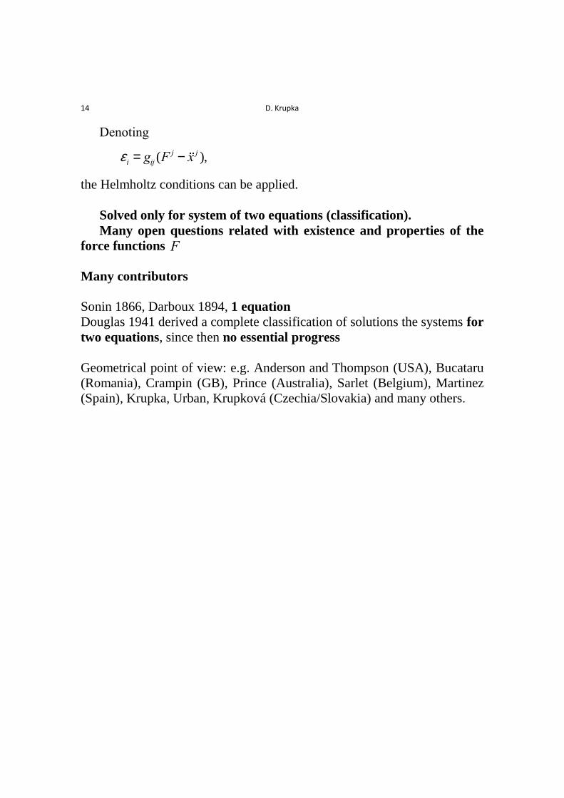
Denoting

e i = gij (F

j - x j ),

the Helmholtz conditions can be applied.

Solved only for system of two equations (classification).

Many open questions related with existence and properties of the

force functions F

Many contributors

Sonin 1866, Darboux 1894, 1 equation

Douglas 1941 derived a complete classification of solutions the systems for

two equations, since then no essential progress

Geometrical point of view: e.g. Anderson and Thompson (USA), Bucataru

(Romania), Crampin (GB), Prince (Australia), Sarlet (Belgium), Martinez

(Spain), Krupka, Urban, Krupková (Czechia/Slovakia) and many others.

Recent trends in the inverse problem of the...

Documents

Transcript of Recent trends in the inverse problem of the...