Recent Developments in Analysis of Uncertainty in TAM · stochastic linearization method for...

Isaac Elishakoff Florida Atlantic [email protected]

(With Xiaojun Wang, BU,PRC; Yongjian Ren, PRC; Lova Andriamasy EDF-Electricité de France, Paris, France)

11

Recent Developments in

Analysis of Uncertainty in TAM

Uncertain Mechanics = Stochastic Mechanics + Non-Stochastic Mechanics

Non Stochastic Mechanics = Fuzzy Mechanics + Convex Mechanics

22

Dedicated to the

blessed memory

of

Professor

H.D.BUI

Criterion : Minimum mean-square deviation between the original non-linear expression of the force ϕ(X),and the linear counterpart .

(X = displacement, = spring constant of the equivalent linear system)

MULTIPLE COMBINATIONS OF THE STOCHASTIC

LINEARIZATION CRITERIA BY THE MOMENT APPROACH

� 1953 � J.R. Booton

1954 � I.E. Kazakov

1954 � T.K. Caughey

1980 � S.H. Crandall

77

stochastic linearization method for non-linear random vibration

Xkeq

eqk

Stochastic Mechanics

� First criterion

� Second criterion added by Kazakov :

88

[ ] ( )21 XE)X(XEk )(eq ϕ=

Equivalent Spring Constant

[ ] [ ]22 )Xk(E)X(E eq=ϕ

( )222 XE)]X([Ek )(eq ϕ=

Basic Equations

� Single degree of freedom system :

� Method of moments :� substitution of ϕ(X) by

� Error :

� deficiency probabilistically orthogonal to X : =0

=

99

)t(F)X()X(Xm =++ &&& ψϕϕ(X) : non-linear restoring force

: non-linear damping force

m : mass

F(t) : excitation with specified probabilistic properties

)X( &ψ

Xkeq

Xk)X()X( eq−= ϕεϕX),X(ϕε

XX

XXkeq ,

),(ϕ= )(

eqk 1

� Error , between the damping force and its linear replacement :

� = 0

1010

)X( &ψε )X( &ψXceq&

Xc)X()X( eq&&& −=ψεψ

X),X( &&ψε=eqc

)(eqcX,XX),X( 1=&&&&ψ

Second criterion ≈ [ ] ( )

= 22 XcE)X(E eq

&&ψ

[ ] )X(E)X(Ec )(eq

222 &&ψ=

Re-Derivation of Energy Criteria

� New criterion : the potential energy of the system� Potential energy of deformation :

� Potential energy of the associated equivalent linear spring :

Deficiency :

Moments method � = 0

1111

∫=X

dx)x()X(P0

ϕ

22Xk)X(P eqeq =

22Xk)X(P)X( eqp −=ε

2X),X(pε[ ] )()(2 42)3( XEXPXEkeq =

Another criterion : [ ] ( )

=222 2XkE)X(PE eq

[ ] )())((2 42)4( XEXPEkeq =

X. Zhang

� Criterion based on the complementary energy :

= 0

1212

)X(P)X(X)X(C −= ϕ

22Xk)X(C)X( eqc −=ε

2X),X(pε

Additional criterion :

[ ] ( )222 2XkE)X(CE eq= [ ] )()(2 42)6( XEXCEkeq =

[ ] )X(E)X(CXEk )(eq

225 2=

Linearization of Damping

� Energy dissipation function :

Residual stemming due to the replacement of the damping force �

= 0

1313

∫=X

dz)z()X(D

&

&

0

ψ

22Xc)X(D eqD&& −=ε

2X,D&ε [ ] )X(E)X(DXEc )(

eq423 2 &&&=

Equality of the mean-square values : [ ] ( )

=222 2XcEDE eq

&

[ ] )X(EDEc )(eq

424 2 &=

Probability density

� If is known, we can evaluate and , because :

� Approximation :

=

=

Differential equation known in the random vibration literature

1414

)x(pX eqk eqc

∫∫∞

∞−

∞

∞−

== dx)x(px)X(E,dx)x(xp)X(E XX &&&&

222

)x(p~)x(p XX ≈)X(E 2 2

X~σ

)X(E 2& 2X

~&σ

( ) ( )XeqeqXeqeq~cc,~kk &σσ ==

( ) ( ) )t(FX~cX~kXm XeqXeq =++ &&&&σσ

Criteria Based Upon Approximating Probability

Density� Booton/Kazakov First criterion with approximate probability density

� Potential energies criterion :

minimal

1515

( )[ ] ( )[ ]{ ( )[ ] } 0~~2~~ 2222 =+ϕ−ϕ=−ϕ XeqXeqXeq

eqXeq

kXXEkXEdk

dXkXE

dk

d σσσσ

)(eqk 7

( )[ ] ( )[ ]222 2Xk~XPEPE eqX −= σ∆

( )[ ] ( )[ ]{ ( )[ ] } 04)(~~ 42222 =+−=∆ XEkXPXEkXPEdk

dPE

dk

deqXeqX

eqeq

σσ

)(eqk 8

� Complementary energy criterion :

minimal

1616

( )[ ] ( )[ ]222 2XkXCECE eqX~ −= σ∆

( )[ ] ( )[ ]{ ( )[ ] } 04)(~~ 42222 =+−=∆ XEkXCXEkXCEdk

dCE

dk

deqXeqX

eqeq

σσ

)(eqk 9

� For derivation of :

minimal

�Minimum mean-square difference :

( )[ ] [ ]22 )( XcXEFE eqD&& −=∆ ψ

eqc

( )[ ] ( )[ ]{ ( )[ ] } 04)(~~ 42222 =+−=∆ XEcXDXEcXDEdc

dDE

dc

deqXeqX

eqeq

&&&&&& σσ

)(eqc 8

( ) [ ]2222Xc)~X(ME)X(ME eqX

&&&& −=

σ∆

( )[ ] ( )[ ]{ ( )[ ] ( )[ ] } 04)(~~~)( 422222 =+−−=∆ XEcXMXEXMXEcXMEdc

dXME

dc

deqXXeqX

eqeq

&&&&&&&&&& σσσ

)(eqc 9

Why so many criteria ?� 9 different criteria for evaluating the equivalent stiffness

9 different conditions for evaluating the stiffness coefficient

9² = 81 criteria for nonlinear stochastic problem.

1717

eqk

eqc

So Why ?

Why not !

1818

How can you govern a

country which has 246

varieties of cheese?

Charles De Gaulle, in "Les Mots du

General", 1962

French general & politician (1890 - 1970)

1919

Plenty of criteria to solve linear deterministic problems :

� Methods :

- Numerical integration

- Successive approximations

- Rayleigh-Ritz

- Bubnov-Galerkin

- Petrov-Galerkin

- Finite difference

- Finite elements

- etc.

How to choose ? Accumulation of experience

� Failure criteria :

- Maximum stress

- Maximum strain

- St-Venant's criterion

- Tresca criterion

- Goldenblat-Kopnovcriterion

- Tsai-Wu criterion

- etc.

Acta Mechanica 204, 89-98 (2009)

Isaac Elishakoff . Lova Andriamasy . Melanie Dolley

Application and extension of the stochastic

linearization by Anh and Di Paola

2020

21

General Methodology for

Hybrid Theoretical, Numerical

and Experimental

Analysis of Uncertain Structures

(With Prof. Xiaojun Wang and Prof.

Zhiping QiuInstitute of Solid Mechanics, Beijing University of Aeronautics and

Astronautics)

« Data ! Data ! Data ! »

He cried impatiently.

« I can’t make bricks

without clay. »

22

Sherlock Holmes to Dr. Watson« The Adventure of the Copper Beeches »

23

Two-Sided Approach

Theodorus of Cyrene

24

� Comparisons of Convex Modeling and Interval Analysis through numerical examples

� Convex Analyses for Vibration and Buckling of Composite Shells Based on Experimental Data

� Application and Extension of the Stochastic Linearization by Anh and Di Paola

� Conclusions

Main Contents

25

a. Determine the smallest hyper-rectangle and the smallest ellipsoidcontaining the given experimental data using the Method by Zhu, Elishakoff and Starnes

b. Convex Modeling and Interval Analysis for the Structural Response

c. Seven-Bar Planar Truss Structure (inclusion relation between the derived ellipse and rectangle)

� The principal axes of the derived ellipse and rectangle are parallel to the global coordinate system

� The principal axes of the derived ellipse and rectangle are not parallel to the global coordinate system

d. Sixty-Bar Space Truss Structure (non-inclusion relation between the derived

ellipse and rectangle)

Comparisons of Convex Modeling and Interval Analysi s

26

1 2( , , , )ma a a a= L

( 1, 2, , )ia i m= L

( ) ( 1,2, , )ra r M= LM experimntal points

0 0( ) ( ) 1Ta a W a a− − ≤Convex modeling assumes that all these experimental points belong to an ellipsoid

Uncertain parameters

m-dimensional parameter space

( ) ( 1,2, , )rb r M= L1 2 1( , , , )m mT θ θ θ −L

Transformation matrixRotated coordinate system

Method by Zhu, Elishakoff and Starnes (1)

27

m-dimensional box contains all M points

0b b d− ≤

1 2( , , , )Tmd d d d= L0 10 20 0( , , , )T

mb b b b= L

( )( )

( ) ( )

( ) ( )0

1max( ) min( ) ,

21

max( ) min( ) ,2

r rk k k

rr

r rk k krr

d b b

b b b

= −

= +( 1, 2, , ; 1, 2, , )r M k m= =L L

Vector of central points Vector of semi-axes


28

Enclose the previous box by an ellipsoid2

02

1

( )1

mk k

k k

b b

g=

− ≤∑

1

m

e m kk

V C g=

= ∏Ellipsoid with minimum volume

Volume of an m-dimensional ellipsoid

The semi-axes of the ellipsoid kg

, ( 1,2, , )i ig md i m= = L

Much smaller without experimental points at the corner of the box

kgη

( )2( )0

21

max 1rm

k k

rk k

b b

gη

=

−= ≤∑ ( 1,2, , )r M= L

replaced by


29

Rewrite the ellipsoid in the form

0 0( ) ( ) 1Tb b D b b− − ≤

Rewrite the volume of the ellipsoid

1

mm

e m kk

V C gη=

= ∏( )2 2 2

1 2( ) , ( ) , , ( )mD diag g g gη η η− − −= L

{ }1 2 1

1 2 1, , ,min ( , , , )

me e mV V

θ θ θθ θ θ

−−=

L

L1 2 1( , , , )m mT θ θ θ −L

0 0T

ma T b=T

m mW T DT= 0 0( ) ( ) 1Ta a W a a− − ≤The smallest ellipsoid


30

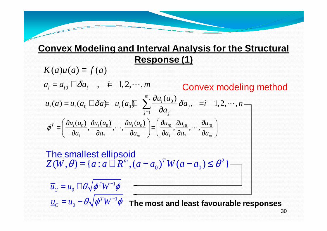
( ) ( ) ( )K a u a f a=

20 0( , ) { : , ( ) ( ) }m TZ W a a R a a W a aθ θ= ∈ − − ≤

0 , 1, 2, ,i i ia a a i mδ= + = L

00 0

1

( )( ) ( ) ( ) , 1,2, ,

mi

i i i jj j

u au a u a a u a a i n

aδ δ

=

∂= + = + =∂∑ L

0 0 0 0 0 0

1 2 1 2

( ) ( ) ( ), , , , , ,T i i i i i i

m m

u a u a u a u u u

a a a a a aϕ

∂ ∂ ∂ ∂ ∂ ∂= = ∂ ∂ ∂ ∂ ∂ ∂ L L

Convex modeling method

The smallest ellipsoid

The most and least favourable responses1

0T

Cu u Wθ ϕ ϕ−= −

10

TCu u Wθ ϕ ϕ−= +

Convex Modeling and Interval Analysis for the Struc tural Response (1)

31

0 0a a a a a− ∆ ≤ ≤ + ∆

00 0

1

( )( ) ( ) ( ) , 1, 2, ,

mi

i i i jj j

u au a u a a u a a i n

aδ δ

=

∂= + = + =∂∑ L

The smallest hyper-rectangle

The most and least favourable responses

00

1

mi

iI i jj j

uu u a

a=

∂= − ∆

∂∑ 00

1

mi

iI i jj j

uu u a

a=

∂= + ∆∂∑

Interval analysis method

Convex Modeling and Interval Analysis for the Struc tural Response (2)

32

y

x

200, 5E A= =

1

2 4

3(0, 0)

(2, 0)

(1, 1) (3, 1)

(4, 0)5

1F 2F

A 7-bar planar truss structure

Seven-Bar Planar Truss Structure

33

Rectangle and ellipse containing the data on uncertain parameters and 1F 2F

0.75 0.85 0.95 1.05 1.15 1.250.85

0.9

0.95

1

1.05

1.1

1.15

F1

F2

3max yCu

3min yCu

3min yIu

3max yIu

Principal axes are parallel to the global coordinat e system : CASE I

34Rectangle and ellipse containing the data on uncertain parameters and

1F 2F

0.85 0.9 0.95 1 1.05 1.1 1.150.9

0.95

1

1.05

1.1

F1

F2

3max yCu

3min yCu

3min yIu

3max yIu

Principal axes are not parallel to the global coordinate system : CASE I

35

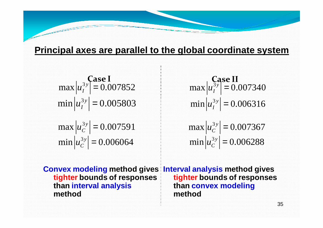
Case I Case II

3min 0.005803yIu =

3max 0.007852yIu =

3min 0.006064yCu =

3max 0.007591yCu =

3min 0.006316yIu =

3max 0.007340yIu =

3min 0.006288yCu =

3max 0.007367yCu =

Interval analysis method gives tighter bounds of responses than convex modeling method

Convex modeling method gives tighter bounds of responses than interval analysis method

Principal axes are parallel to the global coordinat e system

36

Rectangle and ellipse containing the data on uncertain parameters and1F 2F

0.1 0.2 0.3 0.4 0.5 0.61.1

1.2

1.3

1.4

1.5

1.6

F1

F2

3max yCu

3min yCu

3max yIu

3min yIu

Principal axes are parallel to the global coordinat e system : CASE I

37


0.2 0.25 0.3 0.35 0.4 0.45 0.51.25

1.3

1.35

1.4

1.45

1.5

F1

F2

3max yCu

3min yCu

3max yIu

3min yIu

Principal axes are not parallel to the global coordinate system : CASE II

38

Case I Case II



3min 0.004855yIu =

3max 0.006970yIu =

3min 0.004972yCu =

3max 0.006854yCu =

3min 0.005384yIu =

3max 0.006441yIu =

3min 0.005247yCu =

3max 0.006578yCu =

Principal axes are not parallel to the global coordinate system

39

2

2

2

2

2

1

3

123 4

56

78

910

1112

1314

1516

1718

1920

2122 23 24

2F1F

Sixty-Bar Space Truss Structure

40Rectangle and ellipse containing the data on uncertain parameters and

1F 2F

0.24 0.29 0.34 0.39 0.44 0.491.25

1.3

1.35

1.4

1.45

F1

F2

21max xIu

21min xIu

21max xCu

21min xCu

Sixty-Bar Space Truss Structure: Case I

41


0.67 0.72 0.77 0.82 0.87 0.921.08

1.13

1.18

1.23

F1

F2

21max xIu

21min xIu

21max xCu

21min xCu

Sixty-Bar Space Truss Structure: Case II

42

Case I Case II



21min 1.6491E-7xIu =

21max 3.0862E-7xIu =

21min 1.6575E-7xCu =

21max 3.0777E-7xCu =

21min 4.5511E-7xIu =

21max 5.9339E-7xIu =

21min 4.4628E-7xCu =

21max 6.0222E-7xCu =

Sixty-Bar Space Truss Structure

43

Natural frequency

( ) 212 23 13 22 13 23 112

,0 33 211 22 12

21mn

C C C C C C CC

C C Cω

ρ − −

= + −

( )( ) 2

12 23 13 22 13 23 1133 22 2

11 22 12

22

2mn

m n

C C C C C C Cp C p

C C CRλ λ − −

= + ≡ −+

The scatter or uncertainty in elastic moduli influence natural frequency and buckling load

Buckling load

Convex Analysis for Vibration and Buckling of Compo site Shells Based on Experimental Data (1)

N° E1 (GPa) E2 (GPa) v21 G12 (GPa)

1 129.20 9.34 0.28 5.23

2 131.59 9.53 0.33 4.97

3 130.6 9.08 0.33 5.16

4 132.01 9.34 0.33 5.15

5 131.04 8.94 0.34 5.15

6 120.61 9.04 0.33 4.81

7 127.69 8.99 0.32 5.11

8 133.65 9.36 0.35 5.08

9 132.19 9.07 0.30 4.85

10 132.00 9.73 0.35 5.00

11 130.39 9.21 0.34 5.34

12 128.28 8.67 0.33 4.98

13 135.30 9.18 0.32 5.13

14 137.33 9.28 0.33 5.25

15 141.69 10.73 0.31 5.47

16 126.91 9.39 0.33 5.65

17 133.75 9.34 0.32 5.33

18 129.24 9.35 0.3244


Experimental data of the elastic moduli for T300-QY8911

45

Experimental Data for Elastic Moduli

Smallest ellipsoid

Smallest hyper-rectangular

Bounds on and

Convex Modeling Interval Modeling

,0mnω mnp

Ellipsoidal analysis (EA) Interval analysis (IA)

Comparison


46

Case 1: the 10-layer laminated shell, with ply angle being

[ ], , , ,sym

θ θ θ θ θ− − θ ranging from 0o 90o

to

Case 2: the 5-layer laminated shell, with ply angle being

[ ], , , ,θ θ θ θ θ− − θ ranging from 0oto 90o

βThe percentage value defined to quantify the degree of uncertainty of the natural frequency or the critical external pressure of the composite shell as follows

( ) / 2 100%u nlF F Fβ = − ×

where subscripts u, l and n, respectively, denote the upper-bound, lower-bound and the nominal value.

Numerical Examples (1)

47

0 10 20 30 40 50 60 70 80 9065

75

85

95

105

115

125

135

ω11

ω12

ωω ωω (

rad/

sec)

θθθθ (degree)

nominal value lower-bound value of EA upper-bound value of EA lower-bound value of IA upper-bound value of IA

Variability of the fundamental natural frequency for the 10-layer laminated cylindrical shell


48

0 10 20 30 40 50 60 70 80 901

4

7

10

13

16

19

ω11

ω12

p cr (

N/m

2 )

θθθθ (degree)


(×105)

Variability of the critical external pressure for the 10-layer laminated cylindrical shell


49

0 10 20 30 40 50 60 70 80 9034

42

50

58

66

74

ω11

ω12

ωω ωω (

rad/

sec)

θθθθ (degree)


Variability of the fundamental natural frequency for the 5-layer laminated cylindrical shell


50

0 10 20 30 40 50 60 70 80 901

11

21

31

41

ω13

ω11

ω12

p cr (

N/m

2 )

θθθθ (degree)


(×104)

Variability of the critical external pressure for the 5-layer laminated cylindrical shell


51

0 10 20 30 40 50 60 70 80 904.9

5.1

5.3

5.5

5.7

5.9

6.1

6.3

ββ ββ ωω ωω

θθθθ (degree)

β for ellipsoidal analysis β for interval analysis

Degree of uncertainty of the fundamental natural frequency for the 10-layerlaminated cylindrical shell


52

0 10 20 30 40 50 60 70 80 908.5

9.5

10.5

11.5

12.5

13.5

ββ ββ pcr

θθθθ (degree)


Degree of uncertainty of the critical external pressure for the 10-layerlaminated cylindrical shell


53

0 10 20 30 40 50 60 70 80 904.6

5.1

5.6

6.1

6.6

ββ ββ ωω ωω

θθθθ (degree)


Degree of uncertainty of the fundamental natural frequency for the 5-layerlaminated cylindrical shell


54

0 10 20 30 40 50 60 70 80 907.5

8.5

9.5

10.5

11.5

12.5

13.5

14.5

ββ ββ pcr

θθθθ (degree)


Degree of uncertainty of the critical external pressure for the 5-layerlaminated cylindrical shell


Optimization and

Anti-Optimization

of Structures

under

Uncertainty

55

2010World Scientific & Imperial

College Press

56

Recent Work

Superellipsoid (Mr. Yannis Bekel)

Equation:

57

Most Recent Work

Do We Need the Minimum Volume Figure?

(Mr. Fabien Elettro)

58

Nonclassical Linearization Criteria

in Nonlinear Stochastic Dynamics

1. History

2. General Method

3. Potential Energy Linearization

4. Complementary Energy Linearization

5. Comparison of Two Energy Criteria

6. Mean-Square Equality Criteria

59

History

Equality of the mean-squarebetween nonlinear force and its linear counterpart

Non Classical linearizationcriteria based on energy

T.K. Caughey

1959

C. Wang

X.T. Zhang

1985

1991

X.T. Zhang

I. Elishakoff

R.C. Zhang

2001

I. Elishakoff

Bert

G. Ricchiardi

G. Falsone

2003R.C. Booton

1953

1954

I.E. Kazakov

“ […] replace a given set of nonlinear equations by an equivalent set of linear ones; the difference […] is minimized in some appropriate sense.”, Kozin (1987)

I.Elishakoff

2000

2005

L. Socha

60

)(120 tfXkXkXcXm n

n =+++ +•••

(XC( )XP ( ) =XPeq ( )XCeq =

General Method

Oscillator with polynomial nonlinearity :

)( tfXkXcXm eq =++•••

Energies and equivalent energies :

Oscillator with linearized nonlinearity :

)t

( ) ( )∫= dXtXFXP ,

( )∫ tXF ,

( ) ( ) ( )XPXFXXC −= ( ) =XPeq2

2

1Xkeq

( ) ( ) ( )XPXFXXC eqeqeq −=

61

1st Method - Potential Energy Linearization

( ) ( ) 0}]{[ 2 =− neq XXPXPE

( )( ))(1

14

122

0 n

n

neq XE

XEk

nkk

+

++=

Difference of potential energies in the original and replacing system be orthogonal to nX 2

Leads to equivalent stiffness

( )( )122

0 12

1

2

1 +

++ n

n Xkn

Xk 2

2

1Xk eq

62

( ) ( ) 0}]{[ 2 =− neq XXCXCE

( )( ))(1

124

122

0 n

n

neq XE

XEk

n

nkk

+

+++=

2nd Method - Complementary Energy Linearization

Difference potential energies in the original and replacing system be orthogonal tonX 2

Leads to equivalent stiffness

63

With the assumption of normal distribution for we have,

( )tX

)( 20 XEkkk neq α+=

( )

++

+

++

=ionlinearizatenergy ary complementfor ,

1

1214

ionlinearizatenergy potentialfor ,1

14

n

nn

n

n

α

Comparison of Two Energy Criteria (1)

( ) ( ) nn XEnXE )]([!!12 22 −=

giving

Where

)(tfXkXcXm eq =++•••

)(120 tfXkXkXcXm n

n =+++ +•••

( )( ))(1

124

122

0 n

n

neq XE

XEk

n

nkk

+

+++=

64

Mean-square response of the replacing system : ( )eqkc

SXE

π=2

( ) ( ))/(2

1)/(41

0

202 0

kk

XEkkXE

n

n

αα −+

=

( ) ( ) ( )20

20

20

2 )/(4

1XEkkXEXE nα−≈

Comparison of Two Energy Criteria (2)

( ) 1)/(4 20 0 <<XEkk nα

We approximate as follows :

)(tfXkXcXm eq =++•••

)( 20 XEkkk neq α+=

65

Particular Case: Duffing Oscillator

)( 20XE

1

2

3

(1) Exact solution(2) Potential energy criterion(3) Classical stochastic linearization

)(

)(2

2

0XE

XE

Comparison of the exact solution with the potential energy linearization

( ) ( ) ( ) ( )tFtXtXtX =++•••

3αβ

66

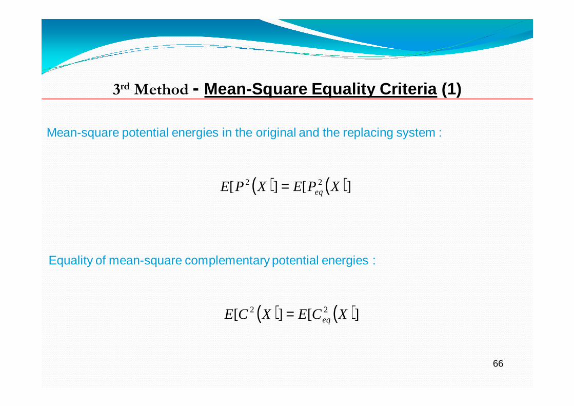
3rd Method - Mean-Square Equality Criteria (1)

( ) ( )][][ 22 XPEXPE eq=

( ) ( )][][ 22 XCEXCE eq=

Mean-square potential energies in the original and the replacing system :

Equality of mean-square complementary potential energies :

67

( )[ ] ( )2

1

2

0

22

2

00 1

+

+= nnnn

eq XEk

kXE

k

kkk γβ

where

( )

( )

+

++

++


3!!)34(

112


!!)34(

1

1

2

2

n

n

n

n

nβ

( )

( )

+

++

++


3

!!)12(

1

)12(2


!!)12(

1

2

n

n

n

n

nγ

3rd Method - Mean-Square Equality Criterias (2)

68

)(

)(2

2

0XE

XE

(a)

(b)

(d)

(c)

)( 20XE

(a) exact solution(b) Equality of mean-squares of potential energies (c) Complementary energy(d) Equality of mean-squares of complementary energies

Contrasts between various energy criteria

Particular Case: Duffing Oscillator

69

� Effectiveness of the energy concepts in the nonlinear stochastic dynamics

� Extension of energy concepts can be performed for the systems with nonlinear

� The applicability of the energy criteria ought to be explored to complex mechanical, civil and aerospace structures

Conclusion

Potential energyMean-squares of potential energiesClassical linearizationComplementary energyMean-squares of complementary energiesac

cura

cy

70

Application and Extension of the

Stochastic Linearization

by Anh and Di Paola

- Anh & Di Paola method

- Atalik & Utku oscillator

- Lutes & Sarkani oscillator

- Mean-Square Equality Criteria

71

Anh & Di Paola method

( ) ( ) ( ) ( )tFtXtXtX =++•••

3αβ

( ) ( ) ( ) ( )tXktXktXktX eqI→→→ 32

51

3α

( ) ( ) ( ) ( )tXktXktXktX eqI→→→ 32

51

3α

vs.

“long shorter way” vs. “short longer way.”

Regulated Gaussian Equivalent Linearization (RGEL)

Anh & Di Paola (1996)

Duffing Oscillator :

72

Atalik & Utku oscillator

( ) ( ) ( ) ( )tFtXtXtX =++•••

3αβ

( ) 2/1/6760.0 dα≈( ) 2/1/5776.0 αd≈2σex

2xσ =

6.14 %

Exact solutionClassical linearization

Anh & Di Paola

?

?

( ) 2/1/6760.0 dα≈( ) 2/1/5776.0 αd≈2σex

2xσ =

Exact solutionClassical linearization

73


Let us apply the RGEL method proposed by Anh & Di Paola

( ) ( ) ( ) ( )tXktXktXktX eqI→→→ 32

51

3α

( ) ( ) ( ) ( ) ( )tFtXtXEtXtX =++•••

][3

7 2αβ

( )tXE ][9 2

α→3

7α9

7α( )tXE ][ 2

Orthogonalization process

74


( ) ( ) ( ) ( )tFtXtXtX =++•••

3αβ

( ) 2/1/6760.0 dα≈ ( ) 2/1/5776.0 αd≈2σex

2xσ =

6.14 %

Exact solution Conventional linearization

Anh & Di Paola

( ) 2/1/ dα2xσ = 0.6546

≈

%17.3Vs.

75

Lutes & Sarkani oscillator

( ) ( ) ( )tFtXtXktX a =+•

)](sgn[

2,exactXσ 2

,approxXclassicalσ ( ) Iregulated tXE ][ 2a Error, % Error, %

1 1 1 0 1 0

2 0.7765 0.7323 5.6877 0.7824 0.7713

3 0.6760 0.5774 14.5904 0.6547 3.1546

4 0.6175 0.4764 22.8490 0.5620 8.9861

5 0.5786 0.4055 29.9225 0.4917 15.0206

6 0.5505 0.3529 35.8981 0.4367 20.6846

7 0.5291 0.3124 40.9630 0.3925 25.8224

( ) ( ) ( ) ( )tXktXktXktXk eqaaa →→→ −

212

1

One-Step Regulation

7 times less

2 times less

15% less

76

Lutes & Sarkani oscillator – Two-Step Regulation

( ) ( ) ( ) ( ) ( ) ( )tXktXktXktXktXktXk IIeqaaaaa

,412

313

212

1 →→→→→ −−−

2,exactXσ 2

,approxXclassicalσ ( ) IIregulated tXE ][ 2

a Error, % Error, %

1 1 1 0 1 0

2 0.7765 0.7824 0.7713 0.8205 5.6693

3 0.6760 0.6547 3.1546 0.7117 5.2820

4 0.6175 0.5620 8.9861 0.6251 1.2229

5 0.5786 0.4917 15.0206 0.5554 4.0131

6 0.5505 0.4367 20.6846 0.4988 9.4038

7 0.5291 0.3925 25.8224 0.4521 14.5548

18 times

Two-Step Regulation = Optimal

77

Conlusion

�Two-step regulation provides an additional improvement. For a=4:

•Classical linearization : 23%•Single-step regulation : 9%•Two-step regulation : 1.23%

�For larger values of a, still much better than the classical or single-step regulation linearization. For a=7:

•Classical linearization : 41%•Single-step regulation : 26%•Two-step regulation : 14.6%

�The method has a large potential and it ought be explored to the wider classes of oscillators

78

Conclusions � The type of the analytical treatment that should be adopted for non-

probabilistic analysis of uncertainty depends upon the available experimental data.

� If V1 is smaller than V2, then one has to prefer interval analysis

� If V1 is in excess of V2, then the analyst ought to utilize convex modeling

� If V1 equals V2 or these two quantities are in close vicinity, then two approaches can be utilized with nearly equal validity

V1 is the minimum volume hyper-rectangle that contains all experimental data

V1 is the minimum volume ellipsoid that contains all experimental data

� The type of the analysis of uncertainty depends on the type and

amount of available information.

79

Conclusions� This study proposes a complete framework for uncertainty analysis in

structures with uncertain parameters. Remarkably, it makes bothellipsoidal modeling and interval analysis as practical tools.

« I am familiar with forty-two different impressions left by tires »

Sherlock Holmes

100100

101101

102102

104104

Charles

Pierre

Baudelaire

(1821 - 1867)

105105

I see better things, and approve,

but I follow worse. VII, 20.

106106

But, since the affairs of men rests still incertain,

Let’s reason with the worst that may befall.

107107

Determinism, like the Queen of England,

reigns -- but does not govern.

Michael Berry

108

I would be pleased to try to

answer your questions

Recent Developments in Analysis of Uncertainty in TAM · stochastic linearization method for...

Documents

Transcript of Recent Developments in Analysis of Uncertainty in TAM · stochastic linearization method for...