Recent Advances on Preserving Methods for General ConservativeSystemsLuigi Brugnano and Felice Iavernaro Citation: AIP Conf. Proc. 1389, 221 (2011); doi: 10.1063/1.3636707 View online: http://dx.doi.org/10.1063/1.3636707 View Table of Contents: http://proceedings.aip.org/dbt/dbt.jsp?KEY=APCPCS&Volume=1389&Issue=1 Published by the American Institute of Physics. Related ArticlesSemi-implicit integration scheme for Landau–Lifshitz–Gilbert-Slonczewski equation J. Appl. Phys. 111, 07D112 (2012) Global weak solutions and smooth solutions for a two-component Hunter-Saxton system J. Math. Phys. 52, 103707 (2011) First numerical investigation of a conjecture by N. N. Nekhoroshev about stability in quasi-integrable systems Chaos 21, 033101 (2011) Integration of nonlinear system of four waves with two velocities in (2 + 1) dimensions by the inverse scatteringtransform method J. Math. Phys. 52, 033504 (2011) Analytic integrability of Hamiltonian systems with a homogeneous polynomial potential of degree 4 J. Math. Phys. 52, 012702 (2011) Additional information on AIP Conf. Proc.Journal Homepage: http://proceedings.aip.org/ Journal Information: http://proceedings.aip.org/about/about_the_proceedings Top downloads: http://proceedings.aip.org/dbt/most_downloaded.jsp?KEY=APCPCS Information for Authors: http://proceedings.aip.org/authors/information_for_authors

Downloaded 05 Oct 2012 to 150.217.1.25. Redistribution subject to AIP license or copyright; see http://proceedings.aip.org/about/rights_permissions

Recent Advances on Preserving Methods for GeneralConservative Systems

Luigi Brugnano∗ and Felice Iavernaro†

∗Dipartimento di Matematica “U. Dini”, Università di Firenze, Italy.†Dipartimento di Matematica “U. Dini”, Università di Bari, Italy.

Abstract. A new class of geometric integrators, able to preserve any number of independent invariants of a general conser-vative problem, is here sketched, by suitably generalizing the line-integral approach which has recently led to the definitionof Hamiltonian BVMs (HBVMs), a class of energy-preserving methods for canonical Hamiltonian systems. Because of thisreason, the new methods are collectively named Line Integral Methods. We here sketch the main results contained in [1].

Keywords: Ordinary differential equations; conservative systems; one-step methods; Hamiltonian Boundary Value Methods; energy-preserving methods; line integral methods.PACS: 00.02.60.Lj; 00.02.60.Cb; 00.02.70.Jn; AMS: 65P10; 65L05.

INTRODUCTION

Energy preserving methods have been the subject of many researches in recent years, mainly related to the numericalsolution of Hamiltonian problems. The first successful attempts to derive energy preserving methods go back to“discrete gradient methods” (see [15, 18] and references therein). More recently, energy preserving Runge-Kuttamethods of order two have been derived in [12], based on the concept of discrete line integral. This idea, furtherdeveloped, has led to fourth order examples of conservative Runge-Kutta methods [13, 14] and, finally, to HamiltonianBoundary Value Methods (HBVMs) [3, 2, 4, 5, 6, 7, 8], a class of energy-preserving Runge-Kutta methods of anyhigh order. Even though energy-conservation is an important feature for the discrete dynamical system induced bythe methods, many Hamiltonian problems (and, in general, conservative problems) are characterized by the presenceof multiple invariants. Therefore, it makes sense to devise numerical methods able to preserve a number (possiblyall) of them (see also [11]). One successful attempt in this direction has been described in [9, 10], where energy-preserving methods able to preserve also quadratic invariants of canonical Hamiltonian systems are defined andanalysed. Additional examples can be found in [16, 17]. We here provide a general framework for this problem, byconsidering, as a descriptive example, the case of Hamiltonian problems with two invariants, though the procedure isstraightforwardly extended to any conservative problem, and to an arbitrary number of invariants [1]. The frameworkis provided by generalizing the discrete line integral methods resulting into HBVMs. For this reason, we name thenew class of methods collectively Line Integral Methods (LIMs). Among them, the straight generalization of HBVMswill be referred to as Generalized HBVMs (GHBVMs), even though the procedure can be naturally extended to anydiscrete method (e.g., collocation methods), whose solution can be suitably associated with a polynomial. With thispremise, the paper is organized as follows: at first, the basic facts on HBVMs are recalled; subsequently, LIMs arederived and analysed, in particular, the conservative generalizations of HBVMs; finally, a numerical test is reportedwhich compares the behavior of a few well-known geometrical integrators to that of the new formulae.

HAMILTONIAN BVMS

HBVMs are here recalled by using the approach followed in [5, 6], where it is shown that the methods are related to alocal truncated Fourier expansion of the continuous problem. Let then

y′(t) = f (y)≡ J∇H(y(t)), y(0) = y0 ∈ R2m, J ≡

(0 Im−Im 0

)=−JT , (1)

be a canonical Hamiltonian problem, where, for sake of simplicity, the Hamiltonian function H(y) is assumed to beanalytical in a region containing the solution, which is assumed to exist for all t ≥ 0. By expanding the right-hand side

Numerical Analysis and Applied Mathematics ICNAAM 2011AIP Conf. Proc. 1389, 221-224 (2011); doi: 10.1063/1.3636707

© 2011 American Institute of Physics 978-0-7354-0956-9/$30.00

221

Downloaded 05 Oct 2012 to 150.217.1.25. Redistribution subject to AIP license or copyright; see http://proceedings.aip.org/about/rights_permissions

of that equation along an orthonormal polynomial basis {Pi} on the interval [0,1], one obtains:

y′(ch) = ∑j≥0

γ j(y)Pj(c), c ∈ [0,1], γ j(y) =∫ 1

0Pj(τ)J∇H(y(τh))dτ , j ≥ 0. (2)

In order to define a polynomial of given degree, say r, approximating the solution of (1), it is enough to truncate theseries at the right-hand side in (2) after r terms, thus obtaining

σ ′(ch) =r−1

∑j=0

γ j(σ)Pj(c), c ∈ [0,1], γ j(σ) =∫ 1

0Pj(τ)J∇H(σ(τh))dτ , j ≥ 0, (3)

whose (polynomial) solution is implicitly defined by σ(ch) = y0 + h∑r−1j=0 γ j(σ)

∫ c0 Pj(τ)dτ , c ∈ [0,1]. By using a

suitable line integral, one easily realizes that H(σ(h)) = H(y0). In fact,

H(σ(h))−H(y0) = h∫ 1

0∇H(σ(ch))T σ ′(ch)dc = h

r−1

∑j=0

γ j(σ)T Jγ j(σ) = 0, (4)

considering that matrix J is skew-symmetric. Furthermore, the following result can be proved (see, e.g., [6]).

Theorem 1 y(h)−σ(h) = O(h2r+1).

We use a quadrature formula defined at the abscissae {c1, . . . ,ck}, having order of accuracy q (that is, exact forpolynomials of degree at least q−1), to approximate the integrals appearing in (3). One then obtains

u′(ch) =r−1

∑j=0

Pj(c)k

∑�=1

b�Pj(c�) f (u(c�)). (5)

Hereafter, we shall consider a Gaussian quadrature formula, so that q= 2k. Equation (5) defines a HBVM(k,r) methodat the k Gauss-nodes. With such a choice of the nodes, HBVM(r,r) turns out to be the Gauss methods of order 2r[4] (for completeness, we also mention that HBVMs defined at Lobatto nodes were previously considered in [3]).Consequenly, one obtains that σ ≡ u in the case where H is a polynomial of degree no larger than 2k/r. Otherwise, thetwo polynomials will differ. However, by choosing k large enough, a practical conservation of energy can be alwaysobtained. Indeed, the following result hold true (see, e.g., [6]).

Theorem 2 y(h)−u(h) = O(h2r+1), H(y(h))−H(u(h)) = O(h2k+1), ∀k ≥ r.

LINE INTEGRAL METHODS

We now generalize the previous formulae and methods, in order to obtain new ones able to preserve, in the discretesolution, more than one invariant of the continuous dynamical system. For sake of brevity, we shall only discussthe case of two invariants (e.g., the Hamiltonian H(y) and another one, say L(y)), though the argument can bestraightforwardly extended to any number of invariants and, evidently, to any suitable function f (y) in (1). The keyidea is again to exploit the properties of the line integral (and its discrete counterpart), originally used to deriveHBVMs. In more detail, the the dynamical system induced by (1) admits a (smooth) invariant L(y) if and only if,along any trajectory y(t), and for any h > 0, L(y(h))−L(y0) = h

∫ 10 ∇L(y(τh))T y′(τh)dτ = h∑ j≥0 φ j(y)T γ j(y) = 0,

where we have used the expansion (2) and the following one: ∇L(y(ch)) = ∑ j≥0 Pj(c)∫ 1

0 Pj(τ)∇L(y(τh))dτ ≡∑ j≥0 Pj(c)φ j(y), c ∈ [0,1]. Moreover, we shall denote by {ρ j(y)} j≥0 the Fourier coefficients of ∇H(y), namelyρ j(y) = JT γ j(y). With this premise, the variant of HBVMs able to preserve both the invariants, is defined by theformula

σ ′(ch) =r−1

∑j=0

Pj(c)γ j(σ) + P0(c)(x1ρ0(σ)+ x2φ0(σ)) , c ∈ [0,1], (6)

in place of (3). The coefficients x1,x2 are then chosen in order to obtain the conservation conditions H(σ(h)) = H(y0)and L(σ(h)) = L(y0). Under mild assumptions, this can be always achieved, thus obtaining that Theorem 1 continuesformally to hold (we refer to [1] for full details). The discretization issue then proceeds as for the previous case, byapproximating the integrals defining the Fourier coefficients by a suitable quadrature rule at the abscissae {c1, . . . ,ck}.The resulting polynomial approximation, say u(ch), still satisfies Theorem 2 for any invariant, besides H(y), when thek abscissae are placed at the Gauss points on [0,1]: this conservative method will be referred to as GHBVM(k,r).

222

Downloaded 05 Oct 2012 to 150.217.1.25. Redistribution subject to AIP license or copyright; see http://proceedings.aip.org/about/rights_permissions

A NUMERICAL TEST

The Kepler problem, defined by the Hamiltonian function H(y) ≡ H(q1,q2, p1, p2) =12

(p2

1 + p22

)−

(q2

1 +q22

)− 12 ,

admits three independent first integrals: the Hamiltonian itself, the total angular momentum, M(y)≡ L(q1,q2, p1, p2) =

q1 p2−q2 p1, and the Laplace-Runge-Lenz (LRL) vector, A(y)≡ A(q1,q2, p1, p2) = q2 p21−q1 p1 p2−q2

(q2

1 +q22

)− 12 .

Since the phase space has dimension four, any integrator that preserves all these invariants has the property to generatea discrete orbit that lies on the very same continuous orbit (an ellipse) of the original problem.

The aim of the present test is to compare a few geometrical integrators on the basis of their qualitative properties inreproducing a consistent phase portrait. In particular, since for h small all the integrators we use would produce goodresults, we are interested in using an as large as possible stepsize h and see how the choice of h affects the stabilityproperties of the corresponding numerical solution.

We consider the following methods of order four: GHBVM(10,2) described above, which yields a conservation ofthe three first integrals within machine precision; the energy-conserving method HBVM(10,2), and the (symplectic)Gauss method of order four (GAUSS4). For comparison reasons we also consider the Symplectic Euler method andthe Störmer–Verlet method.

We first integrate the problem on the time interval [0,300], with stepsize h = 0.03 and initial condition y0 =

[ 110 , 0, 0,

√1.90.1 ]

T which yields an ellipse with eccentricity e = 0.9 and major-axis d = 2. As is clear from the left

picture of Figure 1 the GHBVM(10,2) faithfully reproduces such an ellipse in the (q1,q2)-plane. The HBVM(10,2)introduces a sham rotation of the plane but does not deform the shape of the ellipse. This is also deduced from the rightpicture of Figure 1 that reports the distance of the moving point from the focus located at the origin O: the oscillationsproduced by the HBVM are uniform and there is no relevant difference from the analogous plot for the GHBVM. Onthe contrary, the solution produced by GAUSS4, though bounded (at least on the selected time window), displays anirregular behaviour and the ellipse, while rotating, undergoes repentine deformations (see the bottom-right plot).

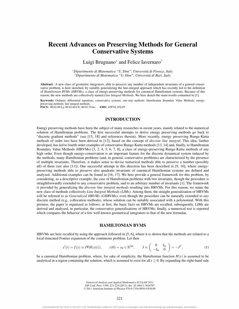
Finally, we compute the average major axes of the elliptical shaped orbits, and display the corresponding absoluteerror as a function of the stepsize h ∈ [0.001, 0.05] (see Figure 2). The two explicit methods evidently have poorerstability properties if compared to the three implicit methods: they tend to strongly enlarge the theoretical ellipse andthe numerical solutions they provide become unbounded for moderate values of the stepsize h (the two lines break forvalues of h as larger as 0.02). The solution provided by GAUSS4 is unbounded for h larger than 0.035 and, beforethat critical value, yields oscillations that differ significantly from the original ones in amplitude. The HBVM and theGHBVM produce comparable results: since we have considered the same integration interval independently of h, amoderate growth of the error is rightly expected as h increases, due to the numerical procedures that approximate theellipses enveloping the numerical orbit at each oscillation around the focus.

−2.5 −2 −1.5 −1 −0.5 0 0.5−2

−1.5

−1

−0.5

0

0.5

HBVM(10,2)

GAUSS4

GHBVM(10,2)

0 50 100 150 200 250 3000

1

2

0 50 100 150 200 250 3000

1

2

0 50 100 150 200 250 3000

1

2

GHBVM

HBVM

GAUSS

FIGURE 1.

223

Downloaded 05 Oct 2012 to 150.217.1.25. Redistribution subject to AIP license or copyright; see http://proceedings.aip.org/about/rights_permissions

0 0.005 0.01 0.015 0.02 0.025 0.03 0.035 0.04 0.045 0.0510

−6

10−5

10−4

10−3

10−2

10−1

100

101

Symplectic Euler

Stormer–Verlet

GAUSS4

HBVM(10,2)

GHBVM(10,2)

FIGURE 2.

REFERENCES

1. L. Brugnano, F. Iavernaro. Line Integral Methods able to preserve all invariants of conservative problems. (Preprint) (2011).2. L. Brugnano, F. Iavernaro, D. Trigiante. Hamiltonian BVMs (HBVMs): a family of "drift-free" methods for integrating

polynomial Hamiltonian systems. AIP Conf. Proc. 1168 (2009) 715–718.3. L. Brugnano, F. Iavernaro and D. Trigiante. Analisys of Hamiltonian Boundary Value Methods (HBVMs): a class of energy-

preserving Runge-Kutta methods for the numerical solution of polynomial Hamiltonian dynamical systems, (submitted),(2009) (arXiv:0909.5659).

4. L. Brugnano, F. Iavernaro and D. Trigiante. Hamiltonian Boundary Value Methods (Energy Preserving Discrete Line IntegralMethods), Jour. of Numer. Anal. Industr. and Appl. Math. 5,1–2 (2010) 17–37. (arXiv:0910.3621)

5. L. Brugnano, F. Iavernaro and D. Trigiante. Numerical Solution of ODEs and the Columbus’ Egg: Three Simple Ideas forThree Difficult Problems. Mathematics in Engineering, Science and Aerospace 1,4 (2010) 105–124. (arXiv:1008.4789)

6. L. Brugnano, F. Iavernaro and D. Trigiante. A unifying framework for the derivation and analysis of effective classes ofone-step methods for ODEs, (submitted) (2010) (arXiv:1009.3165).

7. L. Brugnano, F. Iavernaro and D. Trigiante. A note on the efficient implementation of Hamiltonian BVMs. Jour. Comput. Appl.Math. (accepted).

8. L. Brugnano, F. Iavernaro and D. Trigiante. The Lack of Continuity and the Role of Infinite and Infinitesimalin Numerical Methods for ODEs: the Case of Symplecticity. Applied Mathematics and Computation (accepted)doi:10.1016/j.amc.2011.03.022

9. L. Brugnano, F. Iavernaro and D. Trigiante. On the Existence of Energy-Preserving Symplectic Integrators Based upon GaussCollocation Formulae, (sumbitted) (2010) (arXiv:1005.1930).

10. L. Brugnano, F. Iavernaro and D. Trigiante. Energy and quadratic invariants preserving integrators of Gaussian type, AIP Conf.Proc. 1281 (2010) 227–230. (arXiv:1008.4790)

11. M. Calvo, M.P. Laburta, J.I. Montijano, L. Rández. Error growth in the numerical integration of periodic orbits. Math. Comput.Simul. To appear (2011) doi:10.1016/j.matcom.2011.05.007.

12. F. Iavernaro, B. Pace. s-Stage Trapezoidal Methods for the Conservation of Hamiltonian Functions of Polynomial Type. AIPConf. Proc. 936 (2007) 603–606.

13. F. Iavernaro and B. Pace, Conservative Block-Boundary Value Methods for the solution of Polynomial Hamiltonian Systems,AIP Conf. Proc. 1048 (2008) 888–891.

14. F. Iavernaro and D. Trigiante. High-order Symmetric Schemes for the Energy Conservation of Polynomial HamiltonianProblems, Jour. of Numer. Anal., Ind. and Appl. Math. 4,1–2 (2009) 87–101.

15. R.I .McLachlan, G.R.W. Quispel, N. Robidoux. Geometric integration using discrete gradient. Phil. Trans. R. Soc. Lond. A357 (1999) 1021–1045.

16. G.R.W. Quispel, H.W. Capel. Solving ODE’s numerically while preserving a first integral, Phys. Lett. A 218 (1996) 223–228.17. G.R.W. Quispel, H.W. Capel. Solving ODEs numerically while preserving all first integrals. Preprint (1999).18. G.R.W. Quispel, D.I. McLaren. A new class of energy-preserving numerical integration methods. J. Phys. A: Math. Theor. 41

(2008) 045206 (7pp).

224

Downloaded 05 Oct 2012 to 150.217.1.25. Redistribution subject to AIP license or copyright; see http://proceedings.aip.org/about/rights_permissions