Rebecca Batorsky, Sr. Bioinformatics Specialist at Tufts · Bioinformatics for RNAseq Workshop -...

Bioinformatics for RNAseq Workshop - day 2Bioinformatics for RNAseq Workshop - day 2Rebecca Batorsky, Sr. Bioinformatics Specialist at TuftsRebecca Batorsky, Sr. Bioinformatics Specialist at Tufts

April 2019April 2019

1 / 621 / 62

While you are waiting, please:Download day 1 slides from: https://sites.tufts.edu/biotools/

Tutorials -> bioinformatics_rnaseq_workshop_day_2

In a Chrome web browser: https://ondemand.cluster.tufts.edu

Login with your tufts credentials

2 / 62

https://sites.tufts.edu/biotools/

https://ondemand.cluster.tufts.edu/

Today's Schedule1. Viewing alignment in IGV

2. R and Rstudio Introduction

3. Differential Expression Analysis with DESeq2

We'll follow closely some courses from Harvard Chan School Bioinformatics Core(developers of BCBIO)

https://github.com/hbc/NGS_Data_Analysis_Course/ https://hbctraining.github.io/DGE_workshop/

See their pages for many useful tutorials

3 / 62

https://github.com/hbc/NGS_Data_Analysis_Course/

https://hbctraining.github.io/DGE_workshop/

Summary

4 / 62

Why switch to R programming language?

5 / 62

1. Chrome web browserhttps://ondemand.cluster.tufts.edu

2. Choose Rstudio from theInteractive Apps Menu

3. Choose

Number of hours: 4Number of cores: 1Amount of Memory: 32 GbR version: 3.5.0

4. Press "Connect to Rstudio"

Rstudio on the Tufts HPC cluster via "On Demand"

6 / 62

https://ondemand.cluster.tufts.edu/

Rstudio Interface

Go to the File menu -> New File -> R Script, you should see:

File menu -> Save your file as intro.R7 / 62

Testing some commands

In the script editor type the following and click "Run". To run a block of code,highlight it and click "Run"

To see your current working directory

getwd()

"/cluster/kappa/90-days-archive/bio/tools/training/<your user name>/bioinformatics-rnaseq"

To change to our workshop directory

setwd('~/bioinformatics-rnaseq/')

Set some variables

x = 3y = 5z = x + y

Check that the variables appear in the Environment panel

8 / 62

R librariesCheck which paths on the cluster R will use to find library locations:

.libPaths()

Will output the library paths:

[1] "/opt/shared/R/3.5.0/lib64/R/library"

Add a custom library path, which contains libraries that we'll use:

.libPaths('/cluster/tufts/bio/tools/R_libs/3.5')

Load a library:

library(tidyverse)

9 / 62

VectorsA vector is the most basic data structure in R

numbers <- c(1,2,3,4)letters <- c("A","B","C","D")

Vectors must contain all the same type of data If you give a combination, R willcoerce it into one type

combination <- c("A","B",1,2)

combination

[1] "A" "B" "1" "2"

10 / 62

View data frame

meta

conditionSNF2_rep1 SNF2SNF2_rep2 SNF2SNF2_rep3 SNF2SNF2_rep4 SNF2SNF2_rep5 SNF2WT_rep1 WTWT_rep2 WTWT_rep3 WTWT_rep4 WTWT_rep5 WT

View in a new tab

View(meta)

Data FramesData frames are the most common data structure for tables

Read in the metadata for our experiment:

meta <- read.table("data/sample_info.txt", header=TRUE)

11 / 62

View the new table:

meta

condition numberSNF2_rep1 SNF2 1SNF2_rep2 SNF2 2SNF2_rep3 SNF2 3SNF2_rep4 SNF2 4SNF2_rep5 SNF2 5WT_rep1 WT 6WT_rep2 WT 7WT_rep3 WT 8WT_rep4 WT 9

Manipulating Data Frames

The dollar sign $ can be used to select columns in the data frame:

meta$condition

[1] SNF2 SNF2 SNF2 SNF2 SNF2 WT WT WT WT WT Levels: SNF2 WT

To add a column to a data frame

1. create a vector with 10 values

number <- c(1,2,3,4,5,9,8,7,6,10)

2. use $ on the left side:

meta$number <- number

12 / 62

Sorting and �ltering data frames

Another way to select from a data frame is using the sytax

dataframe[rows, columns]

For example, to select the first row and first two columns:

meta[1,1:2]

condition numberSNF2_rep1 SNF2 1

To select the whole first column just least the row number blank (this is the same asmeta$condition):

meta[ ,1]

[1] SNF2 SNF2 SNF2 SNF2 SNF2 WT WT WT WT WT Levels: SNF2 WT

13 / 62

Sorting and �ltering data frames

We can check for rows of our data frame that have a condition satisfied:

meta$number > 5

[1] FALSE FALSE FALSE FALSE FALSE TRUE TRUE TRUE TRUE TRUE

Then, we can use this to filter our data frame for these rows using which:

meta[which(meta$number > 5), ]

We can filter for multiple conditions by using the & operator:

meta[which(meta$number > 5 & condition = "WT"), ]

condition numberWT_rep1 WT 9WT_rep2 WT 8WT_rep3 WT 7WT_rep4 WT 6WT_rep5 WT 10

14 / 62

Data frame recap:

Data frames have row names and columns

condition numberSNF2_rep1 SNF2 1SNF2_rep2 SNF2 2SNF2_rep3 SNF2 3SNF2_rep4 SNF2 4SNF2_rep5 SNF2 5WT_rep1 WT 9WT_rep2 WT 8WT_rep3 WT 7WT_rep4 WT 6WT_rep5 WT 10

Filtering can done by selecting a row and column dataframe[rows, columns], where rowsand columns can be specified as either numbers or binary strings.

15 / 62

Exercise ( 5 minutes) Load the metadata for our experiment that we saw in day 1:

meta_2 <- read.table('data/ERP004763_info.txt', header=T)

Look at the column names and values using View().

Then, repeat the exercise we did yesterday where you filter the data frame for onlyrows corresponding to WT replicate 1.

16 / 62

ggplot = "Grammar of Graphics"

ggplot(): create data objectaes (): "how" the data will lookgeom_point/bar/line: "what" theplot will be

Plotting example with ggplot2

Create a data frame with count values that span 6 orders of magnitude

library(ggplot2)x <-c(1,2,3,4,5,6)counts <-c(1,10,100,1000,10000, 100000)genotype <-c('WT','WT','WT','SNF2','SNF2','SNF2')df <-data.frame(x,counts,genotype)

To generate a basic dot plot:

ggplot(df) + geom_point(aes(x=x,y=counts))

17 / 62

Plotting example with ggplot2To see the relationships more clearly, we'll set the y log scale:

ggplot(df) + geom_point(aes(x=x,y=counts)) + scale_y_log10()

To color by the genotype value:

ggplot(df) + geom_point(aes(x=x, y=counts, color=genotype)) + scale_y_log10()

18 / 62

Exercise ( 5 minutes)

Construct another data frame which has an additional column called "phenotype"which can be either "sick" or "healthy". Make the same plot but add anotherargument shape=phenotype to the aesthetic (aes).

19 / 62

Di�erential Expression with DESeq2

A common goal for RNAseq analysis is to identify genes that are differentiallyexpressed between conditions

https://hbctraining.github.io/DGE_workshop20 / 62

DESeq2: Work�ow overview


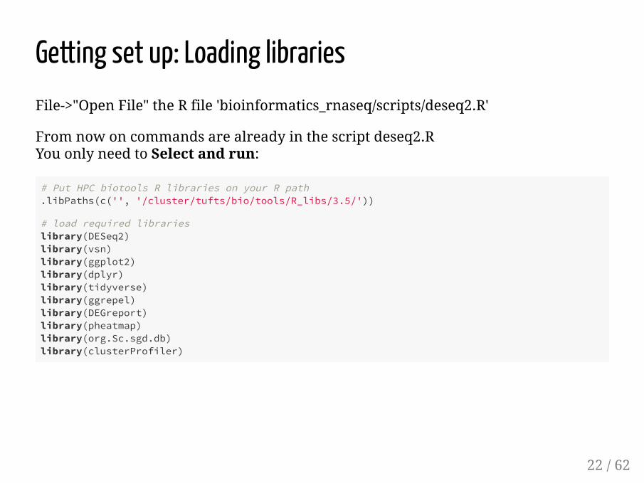
Getting set up: Loading librariesFile->"Open File" the R file 'bioinformatics_rnaseq/scripts/deseq2.R'

From now on commands are already in the script deseq2.R You only need to Select and run:

# Put HPC biotools R libraries on your R path.libPaths(c('', '/cluster/tufts/bio/tools/R_libs/3.5/'))

# load required librarieslibrary(DESeq2)library(vsn) library(ggplot2)library(dplyr)library(tidyverse)library(ggrepel)library(DEGreport)library(pheatmap)library(org.Sc.sgd.db)library(clusterProfiler)

22 / 62

Reading in dataLoad preprocessed data set of 5 WT replicates and 5 SNF2 knockouts

## Read in preprocessed count and meta datacourse_data_path="~/bioinformatics-rnaseq/data/"setwd(course_data_path)data <- read.table("sacCerfeatureCounts_gene_results.formatted.txt",header=TRUE)meta <- read.table("sample_info.txt", header=TRUE)

## View table in new windowView(data)View(meta)

View the first few lines of "data" and "meta" using head() or open the files inanother tab using View()

23 / 62

Create DESeq2 Dataset objectCheck to make sure that all rows labels in meta are columns in data!

all(colnames(data) == rownames(meta))

Create the dataset and run the analysis

dds <- DESeqDataSetFromMatrix(countData = data, colData = meta, design = ~ condition)dds <- DESeq(dds)

Behind the scenes these steps were run:

estimating size factorsgene-wise dispersion estimatesmean-dispersion relationshipfinal dispersion estimatesfitting model and testing

24 / 62

DESeq2: Design formuladds <- DESeqDataSetFromMatrix(countData = data, colData = meta, design = ~ condition)

The design formula design = ~condition

Tells DESeq2 which factors in the metadata to test

The design can include multiple factors that are columns in the metadata

The factor that you are testing for comes last, and factors that you want toaccount for come first

E.g. To test for differences in condition while accounting for sex and age:

design = ~ sex + age + condition

It's even possible to include time series data and interactions

25 / 62

Normalization


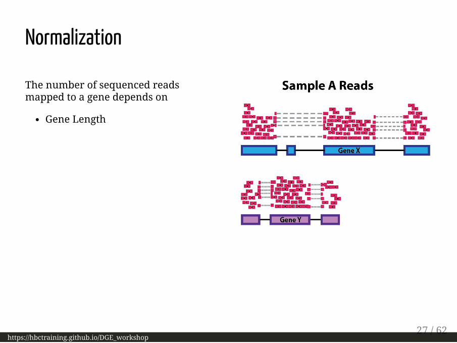
The number of sequenced readsmapped to a gene depends on

Gene Length

Normalization


The number of sequenced readsmapped to a gene depends on:

Gene Length

Sequencing depth

Normalization


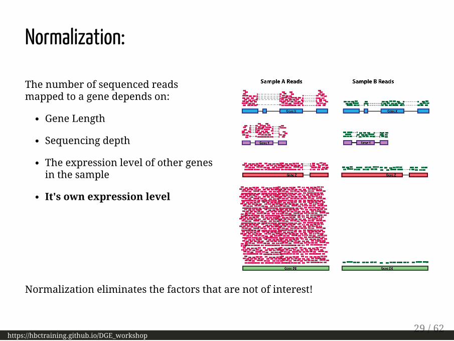
The number of sequenced readsmapped to a gene depends on:

Gene Length

Sequencing depth

The expression level of other genesin the sample

It's own expression level

Normalization:

Normalization eliminates the factors that are not of interest!


Normalization:The naive approach: divide by total library size (CPM, TPM) for each sample is NOTreccomended for comparison between samples

Why not? Reads are a finiate resource and Composition matters!

30 / 62

Normalization:The naive approach: divide by total library size (CPM, TPM) for each sample is NOTreccomended for comparison between samples

Why not? Reads are a finiate resource and Composition matters!

If you only got 10 reads per condition...

condition A condition B

gene 1 5 reads 1 reads

gene 2 5 reads 9 reads31 / 62

Normalization with DESeq2: Median of ratios methodAccounts for both sequencing depth and composition

Step 1: creates a pseudo-reference sample (row-wise geometric mean)

For each gene, a pseudo-reference sample is created that is equal to the geometricmean across all samples.

gene sampleA sampleB pseudo-reference sample

1 1000 1000 = 1000

2 10 1 = 3.16

... ... ... ...

√(1000 ∗ 1000)

√(10 ∗ 1)


Normalization with DESeq2: Median of ratios methodStep 2: calculates ratio of each sample to the reference

Calculate the ratio of each sample to the pseudo-reference. Since most genes aren'tdifferentially expressed, ratios should be similar.

gene sampleA sampleBpseudo-reference

sampleratio of

sampleA/refratio of

sampleB/ref

1 1000 1000 1000 1000/1000 = 1.00 1000/1000 = 1.00

2 10 1 3.16 10/3.16 = 3.16 1/3.16 = 0.32

... ... ... ...

33 / 62

Normalization with DESeq2: Median of ratios methodStep 2: calculates ratio of each sample to the reference

Calculate the ratio of each sample to the pseudo-reference.

gene sampleA sampleBpseudo-reference

sampleratio of

sampleA/refratio of

sampleB/ref

1 1000 1000 1000 1000/1000 = 1.00 1000/1000 = 1.00

2 10 1 3.16 10/3.16 = 3.16 1/3.16 = 0.32

... ... ... ...

Step 3: calculate the normalization factor for each sample (size factor)

The median value of all ratios for a given sample is taken as the normalization factor(size factor) for that sample:

normalization_factor_sampleA <- median(c(1.00, 3.16)) = 2.08 normalization_factor_sampleB <- median(c(1.00, 0.32)) = 0.66

34 / 62

Median should be ~1 for eachsample

This method is robust toimbalance in up-/down-regulation

Normalization with DESeq2: Median of ratios methodVisualization of normalization factor for a sample:


Raw Counts

gene sampleA sampleB

1 1000 1000

2 10 1

Normalized Counts

gene sampleA sampleB

11000/2.08 =

480.771000 / 0.66 =

1515.16

2 10/2.08 = 4.81 1 / 0.66 = 1.52

Median of ratios methodStep 4: calculate the normalized count values using the normalization factor

This is performed by dividing each raw count value in a given sample by thatsample's size factor to generate normalized count values.

SampleA normalization factor = 2.08

SampleB normalization factor = 0.66

36 / 62

Exercise (1 minutes)

View the size factors that were calculated by DESeq2 using your R script:

sizeFactors(dds)

Are they roughly the expected value? Based on these, which sample has the fewestreads and which the largest amount?

37 / 62

Unsupervised Clustering


Unsupervised ClusteringQuality Control step to asses overall similarity between samples:

Which samples are similar to each other, which are different?

Does this fit to the expectation from the experiment’s design?

What are the major sources of variation in the dataset?


Principle Components AnalysisHere is an example with three genes measured in many samples:

gene sampleA sampleB sampleC sampleD ..

1 1000 1000 100 10 ..

2 10 1 5 6 ..

3 10 1 10 20 ..

Each gene that we measure is a "dimension" and we can visualize up to 3 PCA canhelp us visualize relationships in out data in a lower number of dimensions

http://www.nlpca.org/fig_pca_principal_component_analysis.png40 / 62

Make a PCA plotThis uses the built in function plotPCA from DESeq2 (built on top of ggplot)The regularized log transform (rlog) improves clustering by log transforming thedata

rld <- rlog(dds, blind=TRUE)plotPCA(rld, intgroup="condition") + geom_text(aes(label=name))

41 / 62

Exercise (5 minutes)

Does something look wrong with the PCA plot?

Suppose we go back over the data and verify that somewhere in the processingsteps, the data for WT_rep1 and SNF_rep5 columns were switched! Go back and loadthe corrected data frame

data <- read.table("featurecounts_results.formatted.fixed.txt",header=TRUE)

Rerun all steps in the analysis, including the PCA, and verify that things look asexpected.

42 / 62

DESeq2 Work�ow


Modeling count data

DESeq2 will seek to fit a probability distibution to each gene we measured andperform a statistical test to determine whether there is a difference betweenconditions

44 / 62

Since our mean is not equal to thevariance, a Negative binomialdistribution is used

2 parameters NB( , ) mean, dispersion

allows extra source of variation

Modeling count data

This plot shows the relationship between the mean and variance across WTreplicates for each gene we measured:

Dispersion is a measure of spread or variability in the data between biologicalrepliatesGenes with high dispersion will have lower significance than genes with lowdispersion for a given difference between conditions

μ αμ α

45 / 62

Viewing the per-gene dispersion estimatesYou can see the dispersion estimates

plotDispEsts(dds)

46 / 62

Viewing the gene-wise dispersion estimatesWhat DESeq is doing:

1. Estimates dispersion per gene using biological replicates2. Fit a mean-dispersion curve3. Change dispersion estimates for genes that are far from the curveto avoid false

positives

Love et al Genome Biology 201447 / 62

Testing for Di�erential Expression


Creating contrasts and running a Wald testThe null hypothesis: log fold change = 0 for across conditions

P-values are the probability of rejecting the null hypothesis for a given gene, andadjusted p values take into account that we've made many comparisons:

## Creating contrastscontrast <- c("condition", "SNF2", "WT")res_unshrunken <- results(dds, contrast=contrast)summary(res_unshrunken)

out of 6391 with nonzero total read countadjusted p-value < 0.1LFC > 0 (up) : 485, 7.6%LFC < 0 (down) : 637, 10%outliers [1] : 3, 0.047%low counts [2] : 371, 5.8%(mean count < 5)[1] see 'cooksCutoff' argument of ?results[2] see 'independentFiltering' argument of ?results

49 / 62

Shrinkage of the log2 fold changesOne more step where information is used across genes to avoid overestimates ofdifferences between genes with high dispersion


Shrinkage of the log2 fold changesOne more shrinking step - shrink the estimated log2 fold changes This is not done by default, so we run the code:

res <- lfcShrink(dds, contrast=contrast, res=res_unshrunken)


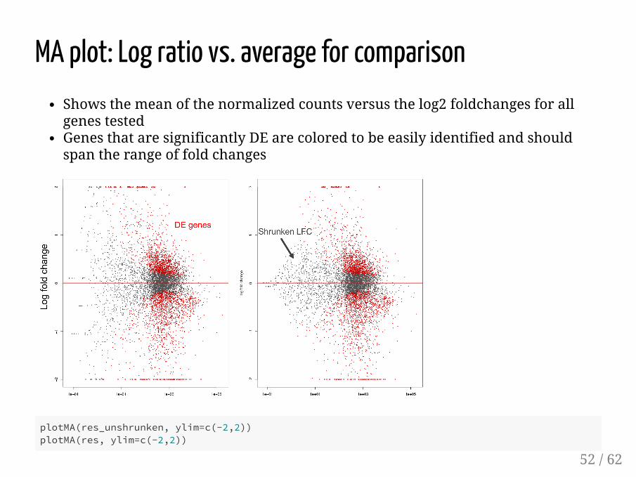
MA plot: Log ratio vs. average for comparisonShows the mean of the normalized counts versus the log2 foldchanges for allgenes testedGenes that are significantly DE are colored to be easily identified and shouldspan the range of fold changes

plotMA(res_unshrunken, ylim=c(-2,2))plotMA(res, ylim=c(-2,2))

52 / 62

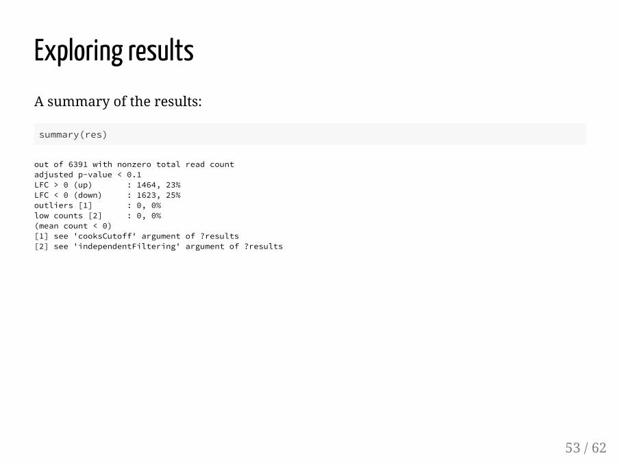
Exploring resultsA summary of the results:

summary(res)

out of 6391 with nonzero total read countadjusted p-value < 0.1LFC > 0 (up) : 1464, 23%LFC < 0 (down) : 1623, 25%outliers [1] : 0, 0%low counts [2] : 0, 0%(mean count < 0)[1] see 'cooksCutoff' argument of ?results[2] see 'independentFiltering' argument of ?results

53 / 62

Exploring resultshead(results)

log2FoldChange = Estimated from the model

padj - Adjusted pvalue for the probability that the log2FoldChange is not zero

log2SNF2Counts

WTCounts

54 / 62

Review DESeq work�owThese comprise the full workflow:

# Setup DESeq2dds <- DESeqDataSetFromMatrix(countData = data, colData = meta, design = ~ condition)# Run size factor estimation, dispersion estimation, dispersion shrinking, testingdds <- DESeq(dds)# Tell DESeq2 which conditions you would like to outputcontrast <- c("condition", "SNF2", "WT")# Output results to tableres_unshrunken <- results(dds, contrast=contrast)# Shrink log fold changes for genes with high dispersionres <- lfcShrink(dds, contrast=contrast, res=res_unshrunken)

55 / 62

Plotting a single gene SNF2 (YOR290C open reading frame)## simple plot for a single geneplotCounts(dds, gene="YOR290C", intgroup="condition")

56 / 62

Filtering to �nd signi�cant genes

Let's filter the results table for padj < 0.05

padj.cutoff <- 0.05 significant_results <- results[which(results$padj < padj.cutoff),]

We can export these results to a table:

file_name='results_pval_0.05.txt'write.table(significant_results, file_name)

57 / 62

Plot multiple genes in a heatmapSort the rows from smallest to largest padj and take the top 50 genes:

significant_results_sorted <- significant_results[order(significant_results$padj), ]significant_genes_50 <- rownames(significant_results_sorted[1:50, ])

We now have a list of genes

significant_genes_50

"YGR234W" "YDR033W" "YOR290C" "YML123C" ...

But we need to find the counts corresponding to these genes. To extract the countsfrom the rlog transformed object

rld_counts <- assay(rld)

Select by row name using the list of genes:

rld_counts_sig <- rld_counts[significant_genes_50, ]

58 / 62

pheatmap(rld_counts_sig, cluster_rows = T, show_rownames = T, annotation = meta, border_color = NA, fontsize = 10, scale = "row", fontsize_row = 8, height = 20)

Plot multiple genes in a heatmappheatmap has many customizable options scale = "row" - mean center each row and divides by the standard deviation to give[-1,1] values

59 / 62

Note on Functional Enrichment

A great tutorial to follow:https://hbctraining.github.io/DGE_workshop/lessons/09_functional_analysis.html

60 / 62

https://hbctraining.github.io/DGE_workshop/lessons/09_functional_analysis.html

What should I do with my �les?Files will remain in the training directory until the end of May, when they will beremoved.

If you have a cluster lab storage space, e.g.:

/cluster/tufts/<your lab name>/<your user name>/

You can copy your work like this:

cd /cluster/tufts/bio/tools/training/your-user-name/cp -r bioinformatics-rnaseq/ /cluster/tufts/your-lab-name/your-user-name/

Otherwise, you can try to copy your data into your home directory, if there's space:

rm ~/bioinformatics-rnaseq #no trailing slashcp -r /cluster/tufts/bio/tools/training/your-user-name/bioinformatics-rnaseq/ ~/

61 / 62

We'd like to hear from you

[email protected] or [email protected]

Short survey by email after course

Thanks for participating!

62 / 62

Rebecca Batorsky, Sr. Bioinformatics Specialist at Tufts · Bioinformatics for RNAseq Workshop -...

Documents

Transcript of Rebecca Batorsky, Sr. Bioinformatics Specialist at Tufts · Bioinformatics for RNAseq Workshop -...