REALIZED GARCH: A JOINT MODEL FOR RETURNS...
30
JOURNAL OF APPLIED ECONOMETRICS J. Appl. Econ. (2011) Published online in Wiley Online Library (wileyonlinelibrary.com) DOI: 10.1002/jae.1234 REALIZED GARCH: A JOINT MODEL FOR RETURNS AND REALIZED MEASURES OF VOLATILITY PETER REINHARD HANSEN, a,b * ZHUO HUANG c AND HOWARD HOWAN SHEK a,d a Department of Economics, Stanford University, Stanford, CA, USA b CREATES, Aarhus, Denmark c China Center for Economic Research, National School of Development, Peking University, Beijing, China d iCME, Stanford University, Stanford, CA, USA SUMMARY We introduce a new framework, Realized GARCH, for the joint modeling of returns and realized measures of volatility. A key feature is a measurement equation that relates the realized measure to the conditional variance of returns. The measurement equation facilitates a simple modeling of the dependence between returns and future volatility. Realized GARCH models with a linear or log-linear specification have many attractive features. They are parsimonious, simple to estimate, and imply an ARMA structure for the conditional variance and the realized measure. An empirical application with Dow Jones Industrial Average stocks and an exchange traded index fund shows that a simple Realized GARCH structure leads to substantial improvements in the empirical fit over standard GARCH models that only use daily returns. Copyright 2011 John Wiley & Sons, Ltd. Supporting information may be found in the online version of this article. 1. INTRODUCTION The latent volatility process of asset returns is relevant for a wide variety of applications, such as option pricing and risk management, and generalized autoregressive conditional heteroskedasticity (GARCH) models are widely used to model the dynamic features of volatility. This has sparked the development of a large number of ARCH and GARCH models since the seminal paper by Engle (1982). Within the GARCH framework, the key element is the specification for conditional variance. Standard GARCH models utilize daily returns (typically squared returns) to extract information about the current level of volatility, and this information is used to form expectations about the next period’s volatility. A single return only offers a weak signal about the current level of volatility. The implication is that GARCH models are poorly suited for situations where volatility changes rapidly to a new level. The reason is that a GARCH model is slow at ‘catching up’ and it will take many periods for the conditional variance (implied by the GARCH model) to reach its new level, as discussed in Andersen et al. (2003). High-frequency financial data are now widely available and the literature has recently introduced a number of realized measures of volatility, including realized variance, bipower variation, the realized kernel, and many related quantities (see Andersen and Bollerslev, 1998; Andersen et al., 2001; Barndorff-Nielsen and Shephard, 2002, 2004; Andersen et al., 2008; Barndorff-Nielsen et al., 2008; Hansen and Horel, 2009; and references therein). Any of these measures is far more informative about the current level of volatility than is the squared return. This makes realized measures very useful for modeling and forecasting future volatility. Estimating a GARCH model Ł Correspondence to: Peter Reinhard Hansen, Department of Economics, Stanford University, 579 Serra all, Stanford, CA 94305-6072, USA. E-mail: [email protected] Copyright 2011 John Wiley & Sons, Ltd.
Transcript of REALIZED GARCH: A JOINT MODEL FOR RETURNS...
JOURNAL OF APPLIED ECONOMETRICSJ. Appl. Econ. (2011)Published online in Wiley Online Library(wileyonlinelibrary.com) DOI: 10.1002/jae.1234
REALIZED GARCH: A JOINT MODEL FOR RETURNSAND REALIZED MEASURES OF VOLATILITY
PETER REINHARD HANSEN,a,b* ZHUO HUANGc AND HOWARD HOWAN SHEKa,d
a Department of Economics, Stanford University, Stanford, CA, USAb CREATES, Aarhus, Denmark
c China Center for Economic Research, National School of Development, Peking University, Beijing,China
d iCME, Stanford University, Stanford, CA, USA
SUMMARYWe introduce a new framework, Realized GARCH, for the joint modeling of returns and realized measures ofvolatility. A key feature is a measurement equation that relates the realized measure to the conditional varianceof returns. The measurement equation facilitates a simple modeling of the dependence between returns andfuture volatility. Realized GARCH models with a linear or log-linear specification have many attractivefeatures. They are parsimonious, simple to estimate, and imply an ARMA structure for the conditionalvariance and the realized measure. An empirical application with Dow Jones Industrial Average stocksand an exchange traded index fund shows that a simple Realized GARCH structure leads to substantialimprovements in the empirical fit over standard GARCH models that only use daily returns. Copyright 2011 John Wiley & Sons, Ltd.
Supporting information may be found in the online version of this article.
1. INTRODUCTION
The latent volatility process of asset returns is relevant for a wide variety of applications, such asoption pricing and risk management, and generalized autoregressive conditional heteroskedasticity(GARCH) models are widely used to model the dynamic features of volatility. This has sparkedthe development of a large number of ARCH and GARCH models since the seminal paper byEngle (1982). Within the GARCH framework, the key element is the specification for conditionalvariance. Standard GARCH models utilize daily returns (typically squared returns) to extractinformation about the current level of volatility, and this information is used to form expectationsabout the next period’s volatility. A single return only offers a weak signal about the currentlevel of volatility. The implication is that GARCH models are poorly suited for situations wherevolatility changes rapidly to a new level. The reason is that a GARCH model is slow at ‘catchingup’ and it will take many periods for the conditional variance (implied by the GARCH model) toreach its new level, as discussed in Andersen et al. (2003).
High-frequency financial data are now widely available and the literature has recently introduceda number of realized measures of volatility, including realized variance, bipower variation, therealized kernel, and many related quantities (see Andersen and Bollerslev, 1998; Andersen et al.,2001; Barndorff-Nielsen and Shephard, 2002, 2004; Andersen et al., 2008; Barndorff-Nielsenet al., 2008; Hansen and Horel, 2009; and references therein). Any of these measures is far moreinformative about the current level of volatility than is the squared return. This makes realizedmeasures very useful for modeling and forecasting future volatility. Estimating a GARCH model
Ł Correspondence to: Peter Reinhard Hansen, Department of Economics, Stanford University, 579 Serra all, Stanford, CA94305-6072, USA. E-mail: [email protected]
Copyright 2011 John Wiley & Sons, Ltd.

P. R. HANSEN, Z. HUANG AND H. H. SHEK
that includes a realized measure in the GARCH equation (known as a GARCH-X model) providesa good illustration of this point. Such models were estimated by Engle (2002), who used therealized variance (see also Forsberg and Bollerslev, 2002). Within the GARCH-X framework noeffort is paid to explain the variation in the realized measures, so these GARCH-X models arepartial (incomplete) models that have nothing to say about returns and volatility beyond a singleperiod into the future.
Engle and Gallo (2006) introduced the first ‘complete’ model in this context. Their modelspecifies a GARCH structure for each of the realized measures, so that an additional latentvolatility process is introduced for each realized measure in the model. The model by Engleand Gallo (2006) is known as the multiplicative error model (MEM), because it builds on theMEM structure proposed by Engle (2002). Another complete model is the HEAVY model byShephard and Sheppard (2010), which, in terms of its mathematical structure, is nested in theMEM framework. Unlike the traditional GARCH models, these models operate with multiple latentvolatility processes. For instance, the MEM by Engle and Gallo (2006) has a total of three latentvolatility processes and the HEAVY model by Shephard and Sheppard (2010) has two (or more)latent volatility processes. Within the context of stochastic volatility models, Takahashi et al. (2009)proposed a joint model for returns and a realized measure of volatility. Importantly, the economicand statistical gains from incorporating realized measures in volatility models are typically foundto be large (see, for example, Christoffersen et al., 2010; Dobrev and Szerszen, 2010).
In this paper we introduce a new framework that combines a GARCH structure for returns withan integrated model for realized measures of volatility. Models within our framework are calledRealized GARCH models, a name that transpires both the objective of these models (similar toGARCH) and the means by which these models operate (using realized measures).
To illustrate our framework and fix ideas, consider a canonical version of the Realized GARCHmodel that will be referred to as the RealGARCH(1,1) model with a linear specification. Thismodel is given by the following three equations:
rt D√htzt,
ht D ω C ˇht�1 C �xt�1,
xt D � C ϕht C ��zt�C ut
where rt is the return, xt a realized measure of volatility, zt ∼ i.i.d.�0, 1�, ut ∼ i.i.d.�0, �2u �, and
ht D var�rtjFt�1� with Ft D ��rt, xt, rt�1, xt�1, . . .�. The last equation relates the observed realizedmeasure to the latent volatility and is therefore called the measurement equation. This equationis natural when xt is a consistent estimator of the integrated variance, because the integratedvariance may be viewed as the conditional variance plus a random innovation. The latter is, inour model, absorbed by ��zt�C ut. It is easy to verify that ht is an autoregressive process oforder one, ht D C ht�1 C wt�1, where D ω C ��, D ˇ C ϕ� , and wt D ���zt�C �ut. Thusit is natural to adopt the nomenclature of GARCH models. The inclusion of the realized measurein the model and the fact that xt has an autoregressive moving average (ARMA) representationmotivate the name Realized GARCH. A simple yet potent specification of the leverage function is��z� D �1z C �2�z2 � 1�, which can generate an asymmetric response in volatility to return shocks.The simple structure of the model makes the model easy to estimate and interpret, and leads to atractable analysis of the quasi maximum likelihood estimator. The framework allows us to use arealized measure that is computed from a shorter period (e.g. 6.5 hours) than the interval that theconditional variance refers to (e.g. 24 hours). In such instances we should expect ϕ < 1.
Copyright 2011 John Wiley & Sons, Ltd. J. Appl. Econ. (2011)DOI: 10.1002/jae
REALIZED GARCH
We apply the Realized GARCH framework to Dow Jones Industrial Average (DJIA) stocks andan exchange traded index fund, SPY. We find, in all cases, substantial improvements in the log-likelihood function (both in-sample and out-of-sample) when benchmarked to a standard GARCHmodel. This is not too surprising, because the standard GARCH model is based on a more limitedinformation set that only includes daily returns. The empirical evidence strongly favors inclusionof the leverage function, and the parameter estimates are remarkably similar across stocks.
The paper is organized as follows. Section 2 introduces the Realized GARCH framework as anatural extension to GARCH. We focus on linear and log-linear specification and show that squaredreturns, the conditional variance, and realized measures have ARMA representations in this classof Realized GARCH models. Our Realized GARCH framework is compared to MEM and relatedmodels in Section 3. Likelihood-based inference is analyzed in Section 4, where we derive theasymptotic properties of the quasi-maximum likelihood estimator (QMLE). Our empirical analysisis given in Section 5. We estimate a range of Realized GARCH models using time series for 28stocks and an exchange-traded index fund. In Section 6 we derive results related to forecastingand the skewness and kurtosis of returns over one or more periods. The latter shows that theRealized GARCH is capable of generating substantial skewness and kurtosis. Concluding remarksare given in Section 7, and the Appendix presents all proofs.
2. REALIZED GARCH
In this section we introduce the Realized GARCH model. The key variable of interest is theconditional variance, ht D var�rtjFt�1�, where frtg is a time series of returns. In the GARCH(1,1)model the conditional variance, ht, is a function of ht�1 and r2
t�1. In the present framework, htwill also depend on xt�1, which represents a realized measure of volatility, such as the realizedvariance. More generally, xt will denote a vector of realized measures, such as the realized variance,bipower variation, intraday range, and squared return. A measurement equation, which ties therealized measure to the latent volatility, ‘completes’ the model. Thus the Realized GARCH modelfully specifies the dynamic properties of both returns and the realized measure.
To simplify the exposition we will assume E�rtjFt�1� D 0. A more general specifications forthe conditional mean, such as a constant or the GARCH-in-mean by Engle et al. (1987), isaccommodated by reinterpreting rt as the return less its conditional mean. The general frameworkfor the Realized GARCH model is presented next.
2.1. The General Formulation
The general structure of the RealGARCH(p, q) model is given by
rt D√htzt �1�
ht D v�ht�1, . . . , ht�p, xt�1, . . . , xt�q� �2�
xt D m�ht, zt, ut� �3�
where zt ∼ i.i.d.�0, 1� and ut ∼ i.i.d.�0, �2u �, with zt and ut being mutually independent.
We refer to the first two equations as the return equation and the GARCH equation, andthese define a class of GARCH-X models, including those that were estimated by Engle (2002),Barndorff-Nielsen and Shephard (2007), and Visser (2011). The GARCH-X acronym refers to thethe fact that xt is treated as an exogenous variable. The HYBRID GARCH framework by Chenet al. (2009) includes variants of the GARCH-X models and some related models.
Copyright 2011 John Wiley & Sons, Ltd. J. Appl. Econ. (2011)DOI: 10.1002/jae

P. R. HANSEN, Z. HUANG AND H. H. SHEK
We shall refer to (3) as the measurement equation, because the realized measure, xt, can oftenbe interpreted as a measurement of ht. The simplest example of a measurement equation isxt D ht C ut. The measurement equation is an important component because it ‘completes’ themodel. Moreover, the measurement equation provides a simple way to model the joint dependencebetween rt and xt, which is known to be empirically important. This dependence is modeled thoughthe presence of zt in the measurement equation, which we find to be highly significant in ourempirical analysis.
It is worth noting that most (if not all) variants of ARCH and GARCH models are nested in theRealized GARCH framework. See Bollerslev (2009) for a comprehensive list of such models. Thenesting can be achieved by setting xt D rt or xt D r2
t , and the measurement equation is redundantfor such models, because it is reduced to a simple identity. Naturally, the interesting case is whenxt is a high-frequency-based realized measure, or a vector containing several realized measures.Next we consider some particular variants of the Realized GARCH model.
2.2. Realized GARCH with a Log-Linear Specification
The Realized GARCH model with a simple log-linear specification is characterized by thefollowing GARCH and measurement equations:
log ht D ω C∑p
iD1ˇi log ht�i C
∑q
jD1�j log xt�j �4�
log xt D � C ϕ log ht C ��zt�C ut �5�
where zt D rt/pht ∼ i.i.d.�0, 1�, ut ∼ i.i.d.�0, �2
u �, and ��z� is called the leverage function. Withoutloss of generality we assume E��zt� D 0.
A logarithmic specification for the measurement equation seems natural in this context. Thereason is that (1) implies that
log r2t D log ht C log z2
t �6�
and a realized measure is in many ways similar to the squared return, r2t , albeit a more accurate
measure of ht. It is therefore natural to explore specifications where log xt is expressed as afunction of log ht and zt, such as (5). A logarithmic form for the measurement equation makesit convenient to specify the GARCH equation with a logarithmic form, because this induces aconvenient ARMA structure.
In our empirical application we adopt a quadratic specification for the leverage function, ��zt�.The conditional variance, ht, is adapted to Ft�1. Therefore Ft must be such that xt 2 Ft (unless� D 0). This requirement is satisfied by Ft D ��rt, xt, rt�1, xt�1, . . .�, but Ft could in principlebe an even richer �-field. Also, note that the measurement equation does not require xt to bean unbiased measure of ht. For instance, xt could be a realized measure that is computed with6.5 hours of high-frequency data, while the return is a close-to-close return that spans 24 hours.
An attractive feature of the log-linear Realized GARCH model is that it preserves the ARMAstructure that characterizes some of the standard GARCH models. This shows that the ‘ARCH’nomenclature is appropriate for the Realized GARCH model. For the sake of generality we derivethe result for the case where the GARCH equation includes lagged squared returns. Thus considerthe following GARCH equation:
log ht D ω C∑p
iD1ˇi log ht�i C
∑q
jD1�j log xt�j C
∑q
jD1˛j log r2
t�j �7�
where q D maxif�˛i, �i� 6D �0, 0�g.Copyright 2011 John Wiley & Sons, Ltd. J. Appl. Econ. (2011)
DOI: 10.1002/jae

REALIZED GARCH
Proposition 1. Define wt D ��zt�C ut and vt D log z2t � �, where � D E log z2
t . The RealizedGARCH model defined by (5) and (7) implies
log ht D h Cp_q∑iD1
�˛i C ˇi C ϕ�i� log ht�i Cq∑jD1
��jwt�j C ˛jvt�j�,
log xt D x Cp_q∑iD1
�˛i C ˇi C ϕ�i� log xt�i C wt Cp_q∑jD1
f��˛j C ˇj�wt�j C ϕ˛jvt�jg,
log r2t D r C
p_q∑iD1
�˛i C ˇi C ϕ�i� log r2t�i C vt C
p_q∑jD1
f�i�wt�j � ϕvt�j�� ˇjvt�jg
where h D ω C �ž� C ˛ž�, x D ϕ�ω C ˛ž��C �1 � ˛ž � ˇž��, and r D ω C �ž� C �1 � ˇž �ϕ�ž��, with ˛ž D ∑q
jD1 ˛j, ˇž D ∑piD1 ˇi, and �ž D ∑q
jD1 �j, and the conventions ˇi D �j D ˛j D0 for i > p and j > q.
Thus the log-linear Realized GARCH model implies that log ht is ARMA(p _ q, q � 1), whereaslog r2
t and log xt are ARMA(p _ q,p _ q). If ˛1 D . . . D ˛q D 0, then log xt is ARMA(p _ q,p).From Proposition 1 we see that the persistence of volatility is summarized by a persistence
parameter :
Dp_q∑iD1
�˛i C ˇi C ϕ�i� D ˛ž C ˇž C ϕ�ž
Example 1. For the case p D q D 1 we have log ht D ω C ˇ log ht�1 C � log xt�1 and log xt D� C ϕ log ht C ��zt�C ut, so that log ht ∼ AR(1) and log xt ∼ ARMA(1,1). Specifically log ht Dh C log ht�1 C �wt�1 and log xt D x C log xt�1 C wt � ˇwt�1, where D ˇ C ϕ� .
The measurement equation induces a GARCH structure that is similar to an EGARCH witha stochastic volatility component. Take the case in Example 1 where log ht D h C log ht�1 C���zt�1�C �ut�1. Note that ���zt�1� captures the leverage effects, whereas �ut�1 adds an additionalstochastic component that resembles that of stochastic volatility models. Thus the Realized GARCHmodel can induce a flexible stochastic volatility structure, similar to that in Yu (2008), butdoes in fact have a GARCH structure because ut�1 is Ft�1-measurable. Interestingly, for thepurpose of forecasting (beyond one-step-ahead predictions), the Realized GARCH is much likea stochastic volatility model since future values of ut are unknown. This analogy does not applyto one-step-ahead predictions because the lagged values, ��zt�1� and ut�1, are known at timet � 1.
An obvious advantage of using a logarithmic specification is that it automatically ensures apositive variance. Here it should be noted that the GARCH model with a logarithmic specification,known as LGARCH (see Geweke, 1986; Pantula, 1986; Milhø j, 1987), has some practicaldrawbacks. These drawbacks may explain that the LGARCH is less popular in applied workthan the conventional GARCH model that uses a specification for the level of volatility (seeTerasvirta, 2009). One drawback is that zero returns are occasionally observed, and will causehavoc for the log-specification unless we impose some ad hoc censoring. Within the RealizedGARCH framework, zero returns are not problematic, because log r2
t�1 does not appear in itsGARCH equation.
Copyright 2011 John Wiley & Sons, Ltd. J. Appl. Econ. (2011)DOI: 10.1002/jae

P. R. HANSEN, Z. HUANG AND H. H. SHEK
2.2.1 The Leverage FunctionThe function ��z� is called the leverage function because it captures the dependence betweenreturns and future volatility, a phenomenon that is referred to as the leverage effect. We normalizesuch functions by E��zt� D 0, and we focus on those that have the form
��zt� D �1a1�zt�C . . .C �kak�zt�, where Eak�zt� D 0, for all k
so that the function is linear in the unknown parameters. We shall see that the leverage functioninduces an EGARCH type structure in the GARCH equation, and we note that the functional formused in Nelson (1991), ��zt� D �1z C �C�jztj � Ejztj�, is within this class of leverage functions. Inthis paper we focus on leverage functions that are constructed from Hermite polynomials, i.e.
��z� D �1z C �2�z2 � 1�C �3�z
3 � 3z�C �4�z4 � 6z2 C 3�C . . .
and our baseline choice for the leverage function is a simple quadratic form: ��zt� D �1zt C �2�z2t �
1�. This choice is convenient because it ensures that E��zt� D 0, for any distribution with Ezt D 0and var�zt� D 1. The polynomial form is also convenient in our quasi-likelihood analysis, and inour derivations of the kurtosis of returns generated by this model.
The leverage function ��z� is closely related to the news impact curve (see Engle and Ng,1993), which maps out how positive and negative shocks to the price affect future volatility.We can define the news impact curve by ��z� D E�log htC1jzt D z�� E�log htC1�, so that 100��z�measures the percentage impact on volatility as a function of the Studentized return. From theARMA representation in Proposition 1 it follows that ��z� D �1��z�.
2.3. Realized GARCH with a Linear Specification
In this section we adopt a linear structure that is more similar to the original GARCH model byBollerslev (1986). One advantage of this formulation is that the measurement equation is simple tointerpret in this model. For instance, if xt is computed from intermittent high-frequency data (i.e.over 6.5 hours) whereas rt is a close-to-close return that spans 24 hours, then we would expectϕ to reflect how much of the daily volatility occurs during trading hours. The linear RealizedGARCH model is defined by
xtht D ω C∑p
iD1ˇiht�i C
∑q
jD1�jxt�j, and D � C ϕht C ��zt�C ut
As is the case for the GARCH(1,1) model the RealGARCH(1,1) model with the linearspecification implies that ht has an AR(1) representation ht D �ω C ���C �ˇ C �ϕ�ht�1 C �wt�1,where wt D ut C ��zt� is an i.i.d. process, and that the realized measure, xt, is ARMA(1,1), which isconsistent with the time series properties of realized measures in this context (see Meddahi, 2003).
3. COMPARISON TO RELATED MODELS
In this section we relate the Realized GARCH model to the multiplicative error model (MEM)by Engle and Gallo (2006) and the HEAVY model by Shephard and Sheppard (2010),1 and somerelated approaches.
1 The Realized GARCH model was conceptualized and developed concurrently and independently of Shephard andSheppard (2010). However, in our current presentation of the model we have adopted some terminology from Shephardand Sheppard (2010).
Copyright 2011 John Wiley & Sons, Ltd. J. Appl. Econ. (2011)DOI: 10.1002/jae

REALIZED GARCH
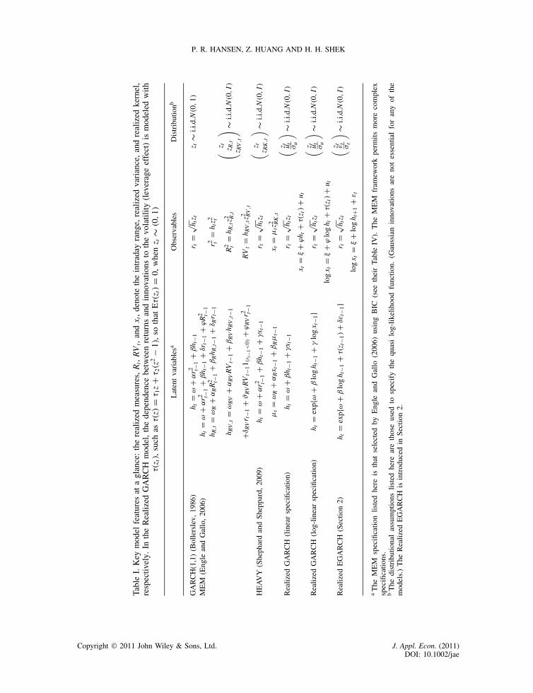
The MEM by Engle and Gallo (2006) utilizes two realized measures in addition to the squaredreturns. These are the intraday range (high minus low) and the realized variance, whereas theHEAVY model by Shephard and Sheppard (2010) uses the realized kernel (RK) by Barndorff-Nielsen et al. (2008). These models introduce an additional latent volatility process for each of therealized measures. Thus the MEM and the HEAVY digress from the traditional GARCH modelsthat only have a single latent volatility factor. Key model features are given in Table I. We haveincluded the level specification of the Realized GARCH model because it is most similar to theGARCH, MEM, and HEAVY models. Based on our empirical analysis in Section 5 we recommendthe log-linear specification in practice.
Brownless and Gallo (2010) estimates a restricted MEM model that is closely related to theRealized GARCH with the linear specification. They utilize a single realized measure, whichleads to two latent volatility processes in their model: ht D E�r2
t jFt�1� and t D E�xtjFt�1�.However, their model is effectively reduced to a single-factor model as they introduce the constraintht D cC dt.
The usual MEM formulation is based on a vector of non-negative random innovations, t,that are required to have mean E� t� D �1, . . . , 1�0. The literature has explored distributions withthis property such as certain multivariate Gamma distributions, and Cipollini et al. (2009) usecopula methods that entail a very flexible class of distributions with the required structure. (Aperhaps simpler way to achieve this structure is by setting t D Zt þ Zt, and working with thevector of mean-zero unit-variance random variables, Zt, instead.) The estimates in Engle andGallo (2006) and Shephard and Sheppard (2010) are based on a likelihood where the elementsof t are independent �2-distributed random variables with one degree of freedom, which mapsinto Zt ∼ N�0, I�. We have used the alternative formulation in Table I so that �z2
t , z2R,t, z
2RV,t�
0corresponds to t in the MEM by Engle and Gallo (2006).
3.1. Multi-factor Realized GARCH Models
The Realized GARCH framework can be extended to a multi-factor structure. For instance, withm realized measures (including the squared return) we could specify a model with k � m latentvolatility factors. The Realized GARCH model introduced in this paper has k D 1, whereas theMEM has m D k. This hybrid framework with 1 � k � m, provides a way to bridge the RealizedGARCH models with the MEM framework. All these models can be viewed as extensions ofstandard GARCH models, where the extensions are achieved by incorporating realized measuresinto the model in various ways.2
4. QUASI-MAXIMUM LIKELIHOOD ANALYSIS
In this section we discuss the asymptotic properties of the quasi-maximum likelihood estimatorwithin the Realized GARCH (p, q) model. The structure of the QMLE analysis is very similarto that of the standard GARCH model (see Bollerslev and Wooldridge, 1992; Lee and Hansen,1994; Lumsdaine, 1996; Jensen and Rahbek, 2004a,b; Straumann and Mikosch, 2006). Both Engleand Gallo (2006) and Shephard and Sheppard (2010) justify the standard errors they report, byreferencing existing QMLE results for GARCH models. This argument hinges on the fact thatthe joint log-likelihood in the MEM is decomposed into a sum of univariate GARCH-X mod-els, whose likelihood can be maximized separately. The factorization of the likelihood is achieved
2 A realized measure simply refers to a statistic that is constructed from high-frequency data. Well-known examples includerealized variance, realized kernel, intraday range, number of transactions, and trading volume.
Copyright 2011 John Wiley & Sons, Ltd. J. Appl. Econ. (2011)DOI: 10.1002/jae
P. R. HANSEN, Z. HUANG AND H. H. SHEK
Tabl
eI.
Key
mod
elfe
atur
esat
agl
ance
:th
ere
aliz
edm
easu
res,Rt,RVt,
andx t
,de
note
the
intr
aday
rang
e,re
aliz
edva
rian
ce,
and
real
ized
kern
el,
resp
ectiv
ely.
Inth
eR
ealiz
edG
AR
CH
mod
el,
the
depe
nden
cebe
twee
nre
turn
san
din
nova
tion
sto
the
vola
tilit
y(l
ever
age
effe
ct)
ism
odel
edw
ith��z t�,
such
as��z�
D� 1z
C� 2�z
2�
1�,
soth
atE��z t�
D0,
whe
nz t
∼�0,1�
Lat
ent
vari
able
saO
bser
vabl
esD
istr
ibut
ionb
GA
RC
H(1
,1)
(Bol
lers
lev,
1986
)h t
Dω
C˛r2 t
�1Cˇh t
�1r t
Dp h
tzt
z t∼
i.i.d
.N�0,1�
ME
M(E
ngle
and
Gal
lo,
2006
)h t
Dω
C˛r2 t
�1Cˇh t
�1Cυrt�
1CϕR
2 t�1
h R,t
DωR
C˛RR
2 t�1
CˇRh R,t
�1Cυ Rr t
�1r2 t
Dh tz2 t
h RV,t
DωRV
C˛RVRVt�
1CˇRVh RV,t
�1R
2 tDh R,tz2 R,t
( zt
z R,t
z RV,t
) ∼i.i
.d.N�0,I�
CυRVr t
�1CϑRVRVt�
11 �r t
�1<
0�CϕRVr2 t
�1RVt
Dh RV,tz2 RV,t
HE
AV
Y(S
heph
ard
and
Shep
pard
,20
09)
h tDω
C˛r2 t
�1Cˇh t
�1C�xt�
1r t
Dp h
tzt
( zt
z RK,t
) ∼i.i
.d.N�0,I�
t
DωR
C˛Rx t
�1CˇRt�
1x t
Dtz
2 RK,t
Rea
lized
GA
RC
H(l
inea
rsp
ecifi
catio
n)h t
Dω
Cˇh t
�1C�xt�
1r t
Dp h
tzt
( z t ut� u
) ∼i.i
.d.N�0,I�
x tD�
Cϕh t
C��z t�
Cu t
Rea
lized
GA
RC
H(l
og-l
inea
rsp
ecifi
catio
n)h t
Dex
pfωCˇ
logh t
�1C�
logx t
�1g
r tD
p htzt
( z t ut� u
) ∼i.i
.d.N�0,I�
logx t
D�
Cϕ
logh t
C��z t�
Cu t
Rea
lized
EG
AR
CH
(Sec
tion
2)h t
Dex
pfω
Cˇ
logh t
�1C��z t
�1�
Cυεt�
1g
r tD
p htzt
( z t ε t � ε) ∼
i.i.d
.N�0,I�
logx t
D�
Clo
gh t
C1Cε t
aT
heM
EM
spec
ifica
tion
liste
dhe
reis
that
sele
cted
byE
ngle
and
Gal
lo(2
006)
usin
gB
IC(s
eeth
eir
Tabl
eIV
).T
heM
EM
fram
ewor
kpe
rmits
mor
eco
mpl
exsp
ecifi
catio
ns.
bT
hedi
stri
butio
nal
assu
mpt
ions
liste
dhe
rear
eth
ose
used
tosp
ecif
yth
equ
asi
log-
likel
ihoo
dfu
nctio
n.(G
auss
ian
inno
vatio
nsar
eno
tes
sent
ial
for
any
ofth
em
odel
s.)
The
Rea
lized
EG
AR
CH
isin
trod
uced
inSe
ctio
n2.
Copyright 2011 John Wiley & Sons, Ltd. J. Appl. Econ. (2011)DOI: 10.1002/jae
REALIZED GARCH
by two facets of these models. One is that all observables (i.e. squared return and each of therealized measures) are being tied to their individual latent volatility process. The other is thatthe primitive innovations in these models are taken to be independent in the formulation of thelikelihood function. The latter inhibits a direct modeling of the leverage effect with a functionsuch as ��zt�, which is one of the traits of the Realized GARCH model. However, in the MEMframework one can generate a leverage type dependence by including suitable realized measuresin various GARCH equations, such as the realized semivariance (see Barndorff-Nielsen et al.,2009b), or by introducing suitable indicator functions as in Engle and Gallo (2006).
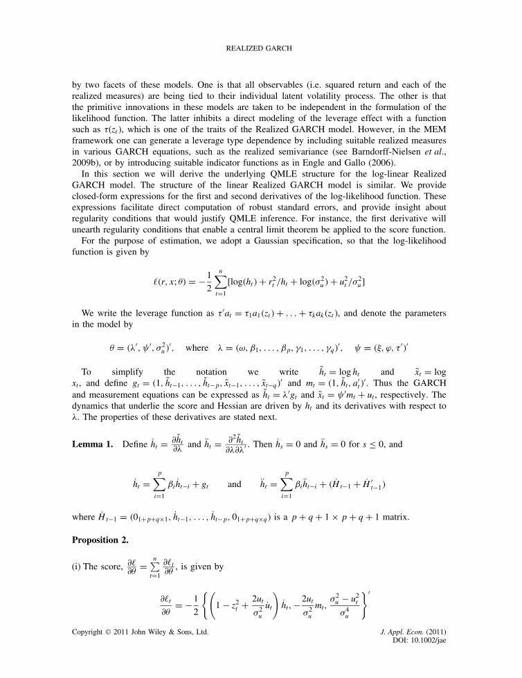
In this section we will derive the underlying QMLE structure for the log-linear RealizedGARCH model. The structure of the linear Realized GARCH model is similar. We provideclosed-form expressions for the first and second derivatives of the log-likelihood function. Theseexpressions facilitate direct computation of robust standard errors, and provide insight aboutregularity conditions that would justify QMLE inference. For instance, the first derivative willunearth regularity conditions that enable a central limit theorem be applied to the score function.
For the purpose of estimation, we adopt a Gaussian specification, so that the log-likelihoodfunction is given by
��r, x; �� D �1
2
n∑tD1
[log�ht�C r2t /ht C log��2
u �C u2t /�
2u ]
We write the leverage function as � 0at D �1a1�zt�C . . .C �kak�zt�, and denote the parametersin the model by
� D ��0, 0, �2u �
0, where � D �ω, ˇ1, . . . , ˇp, �1, . . . , �q�0, D ��, ϕ, � 0�0
To simplify the notation we write Qht D log ht and Qxt D logxt, and define gt D �1, Qht�1, . . . , Qht�p, Qxt�1, . . . , Qxt�q�0 and mt D �1, Qht, a0
t�0. Thus the GARCH
and measurement equations can be expressed as Qht D �0gt and Qxt D 0mt C ut, respectively. Thedynamics that underlie the score and Hessian are driven by ht and its derivatives with respect to�. The properties of these derivatives are stated next.
Lemma 1. Define Pht D ∂ Qht∂� and Rht D ∂2 Qht
∂�∂�0 . Then Phs D 0 and Rhs D 0 for s � 0, and
Pht Dp∑iD1
ˇi Pht�i C gt and Rht Dp∑iD1
ˇi Rht�i C � PHt�1 C PH0t�1�
where PHt�1 D �01CpCqð1, Pht�1, . . . , Pht�p, 01CpCqðq� is a pC q C 1 ð pC q C 1 matrix.
Proposition 2.
(i) The score, ∂�∂� Dn∑tD1
∂�t∂� , is given by
∂�t∂�
D �1
2
{(1 � z2
t C 2ut�2u
Put)
Pht,�2ut�2u
mt,�2u � u2
t
�4u
}0
Copyright 2011 John Wiley & Sons, Ltd. J. Appl. Econ. (2011)DOI: 10.1002/jae
P. R. HANSEN, Z. HUANG AND H. H. SHEK
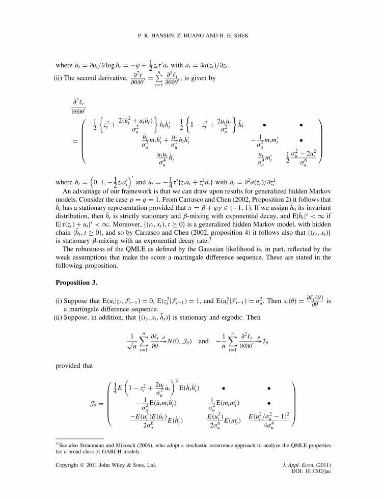
where Put D ∂ut/∂ log ht D �ϕ C 12 zt�
0 Pat with Pat D ∂a�zt�/∂zt.
(ii) The second derivative, ∂2�∂�∂�0 D
n∑tD1
∂2�t∂�∂�0 , is given by
∂2�t∂�∂�0
D
�12
{z2t C 2� Pu2
t C ut Rut��2u
}Pht Ph0
t � 12
{1 � z2
t C 2ut Put�2u
}Rht ž ž
Put�2u
mt Ph0t C ut
�2u
bt Ph0t � 1
�2u
mtm0t ž
ut Put�4u
Ph0t
ut�4u
m0t
12�2u � 2u2
t
�6u
where bt D(
0, 1,�12 zt Pa0
t
)0and Rut D �1
4�0fzt Pat C z2
t Ratg with Rat D ∂2a�zt�/∂z2t .
An advantage of our framework is that we can draw upon results for generalized hidden Markovmodels. Consider the case p D q D 1. From Carrasco and Chen (2002, Proposition 2) it follows thatQht has a stationary representation provided that D ˇ C ϕ� 2 ��1, 1�. If we assign Qh0 its invariantdistribution, then Qht is strictly stationary and ˇ-mixing with exponential decay, and EjQhtjs < 1 ifEj��zt�C utjs < 1. Moreover, f�rt, xt�, t ½ 0g is a generalized hidden Markov model, with hiddenchain fQht, t ½ 0g, and so by Carrasco and Chen (2002, proposition 4) it follows also that f�rt, xt�gis stationary ˇ-mixing with an exponential decay rate.3
The robustness of the QMLE as defined by the Gaussian likelihood is, in part, reflected by theweak assumptions that make the score a martingale difference sequence. These are stated in thefollowing proposition.
Proposition 3.
(i) Suppose that E�utjzt,Ft�1� D 0, E�z2t jFt�1� D 1, and E�u2
t jFt�1� D �2u . Then st��� D ∂�t���
∂� isa martingale difference sequence.
(ii) Suppose, in addition, that f�rt, xt, Qht�g is stationary and ergodic. Then
1pn
n∑tD1
∂�t∂�
d!N�0,J�� and � 1
n
n∑tD1
∂2�t∂�∂�0
p!I�
provided that
J� D
14E
(1 � z2
t C 2ut�2u
Put)2
E� Pht Ph0t� ž ž
� 1�2u
E� Putmt Ph0t�
1�2u
E�mtm0t� ž
�E�u3t �E� Put�
2�6u
E� Ph0t�
E�u3t �
2�6u
E�m0t�
E�u2t /�
2u � 1�2
4�4u
3 See also Straumann and Mikosch (2006), who adopt a stochastic recurrence approach to analyze the QMLE propertiesfor a broad class of GARCH models.
Copyright 2011 John Wiley & Sons, Ltd. J. Appl. Econ. (2011)DOI: 10.1002/jae

REALIZED GARCH
and
I� D
{12 C E� Pu2
t ��2u
}E� Pht Ph0
t� ž 0
� 1�2u
Ef� Putmt C utbt�Ph0tg 1
�2u
E�mtm0t� 0
0 0 12�4
u
are finite.Note that in the stationary case we have J� D E
(∂�t∂�∂�t∂�0
), so a necessary condition for jJ�j < 1
is that zt and ut have finite fourth moments. Additional moments may be required for zt, dependingon the complexity of the leverage function ��z�, because Put depends on ��zt�.
The mathematical structure of the Gaussian quasi log-likelihood function for the RealizedGARCH model is quite similar to the structure analyzed in Straumann and Mikosch (2006).Therefore we conjecture that Straumann and Mikosch (2006, Theorem 7.1) can be adapted to thepresent framework, so that p
n�O�n � �� ! N�0, I�1� J�I�1
� �
To make this result rigorous we would need to adapt and verify conditions N.1–N.4 in Straumannand Mikosch (2006). This is not straightforward and would take up much space, so we leavethis for future research. Moreover, the results in Straumann and Mikosch (2006) only apply tothe stationary case, < 1, so the non-stationary case would have to be analyzed separately usingmethods similar to those in Jensen and Rahbek (2004a,b). For simple ARCH and GARCH models,Jensen and Rahbek (2004a,b) have shown that the QMLE estimator is consistent with a Gaussianlimit distribution regardless of the process being stationary or non-stationary. Therefore, unlikethe case for autoregressive processes, we need not have a discontinuity of the limit distributionat the knife-edge in the parameter space that separates stationary and non-stationary processes. Asimilar result may apply to the Realized GARCH model with the linear specification. However, thelog-linear specification generates a score function with a structure that may result in convergenceto a stochastic integral in the unit root case. We leave this important inference problem for futureresearch.
5. EMPIRICAL ANALYSIS
In this section we present empirical results using returns and realized measures for 28 stocksand and exchange-traded index fund, SPY, that tracks the S&P 500 index. Detailed results arepresented for SPY, whereas our results for the other 28 time series are presented with fewer details,to conserve space. We adopt the realized kernel, introduced by Barndorff-Nielsen et al. (2008),as the realized measure, xt. We estimate the realized GARCH models using both open-to-closereturns and close-to-close returns. High-frequency prices are only available between ‘open’ and‘close’, so the population quantity that is estimated by the realized kernel is directly related to thevolatility of open-to-close returns, but only captures a fraction of the volatility of close-to-closereturns.
We compare the linear and log-linear specifications and argue that the latter is better suitedfor the problem at hand. So we will mainly present empirical results based on the log-linearspecification. We report empirical results for all 29 assets in Table III and find the pointestimates to be remarkably similar across the many time series. In-sample and out-of-samplelikelihood ratio statistics are computed in Table IV. These results strongly favor the inclusionof the leverage function and show that the realized GARCH framework is superior to standard
Copyright 2011 John Wiley & Sons, Ltd. J. Appl. Econ. (2011)DOI: 10.1002/jae

P. R. HANSEN, Z. HUANG AND H. H. SHEK
GARCH models, because the partial log-likelihood of any Realized GARCH model is substantiallybetter than that of a standard GARCH(1,1). This is found to be the case in-sample, as well asout-of-sample.
5.1. Data Description
Our sample spans the period from 1 January 2002 to 31 August 2008, which we divide intoan in-sample period: 1 January 2002 to 31 December 2007; leaving the eight months 2 January2008 to 31 August 2008 for out-of-sample analysis. We adopt the realized kernel as the realizedmeasure, xt, using the Parzen kernel function. This estimator is similar to the well-known realizedvariance, but is robust to market microstructure noise and is a more accurate estimator of thequadratic variation. Our implementation of the realized kernel follows Barndorff-Nielsen et al.(2010) that guarantees a positive estimate, which is important for our log-linear specification. Theexact computation is explained in great detail in Barndorff-Nielsen et al. (2009a). To avoid outliersthat would result from half trading days, we removed days where high-frequency data spanned lessthan 90% of the official 6.5 hours between 9 : 30 a.m. and 4 : 00 p.m. This removes about threedaily observations per year, such as the day after Thanksgiving and days around Christmas. Whenwe estimate a model that involves log r2
t , we deal with zero returns by the truncation max�r2t , ε�
with ε D 10�20. Summary statistics are available as supporting information in a separate WebAppendix.
5.2. Some Notation Related to the Likelihood and Leverage Effect
The log-likelihood function is (conditionally on F0 D ��frt, xt, htg, t � 0�) given by
log L�frt, xtgntD1; �� Dn∑tD1
logf�rt, xtjFt�1�
Standard GARCH models do not model xt, so the log-likelihood we obtain for these modelscannot be compared to those of the Realized GARCH model. However, we can factorize the jointconditional density for �rt, xt� by
f�rt, xtjFt�1� D f�rtjFt�1�f�xtjrt,Ft�1�
and compare the partial log-likelihood, ��r� :Dn∑tD1
logf�rtjFt�1�, with that of a standard GARCH
model. Specifically for the Gaussian specification for zt and ut, we split the joint likelihood intothe sum
��r, x� D �1
2
n∑tD1
[log�2�C log�ht�C r2t /ht]︸ ︷︷ ︸
D��r�
C �1
2
n∑tD1
[log�2�C log��2u �C u2
t /�2u ]
︸ ︷︷ ︸D��xjr�
Asymmetries in the leverage function are summarized by the two statistics �� D corrf��zt�Cut, ztjzt < 0g and �C D corrf��zt�C ut, ztjzt > 0g, which capture the average slope of the newsimpact curve for negative and positive returns.
Copyright 2011 John Wiley & Sons, Ltd. J. Appl. Econ. (2011)DOI: 10.1002/jae

REALIZED GARCH
5.3. Empirical Results for the Linear Realized GARCH Model
Detailed empirical results for the linear specification are available as supporting informationin a separate Web Appendix. We wish to emphasize one empirical observation that concernsthe difference between open-to-close returns and close-to-close returns. With open-to-close SPYreturns our estimates for the RealGARCH(1,1) models are
ht D 0.09�0.05�
C 0.29�0.16�
ht�1 C 0.63�0.18�
xt�1,
xt D �0.05�0.09�
C 1.01�0.19�
ht � 0.02�0.02�
zt C 0.06�0.01�
�z2t � 1�C ut
where the numbers in parentheses are standard errors. Note that the empirical estimates of ϕ and� in the measurement equation are consistent with the belief that the realized kernel is roughly anunbiased measurement of (open-to-close) ht. With close-to-close returns we obtain the followingestimates:
ht D 0.07�0.04�
C 0.29�0.15�
ht�1 C 0.87�0.25�
xt�1,
xt D 0.00�0.08�
C 0.74�0.14�
ht � 0.07�0.02�
zt C 0.03�0.01�
�z2t � 1�C ut
and it is not surprising that the estimate of ϕ is less than one in this case. The point estimate ofϕ suggests that volatility during the ‘open period’ amounts to about 75% of daily volatility.
5.4. Empirical Results for the Log-Linear Realized GARCH Model
In this section we present detailed results for Realized GARCH models with a log-linearspecification of the GARCH and measurement equations. We strongly favor the log-linearspecification over the linear specification for reasons that will be evident in Section 5.5, where wecompare empirical aspects of the two specifications.
5.4.1 Log-Linear Models for SPY (Table II)Table II presents out empirical results for the log-linear specification using six variants of theRealized GARCH model. For the sake of comparison we use the logarithmic GARCH(1,1) modelas the conventional benchmark when comparing the empirical fit in terms of the partial likelihoodfunction (for returns). The left-hand panel has the empirical results for open-to-close SPY returnsand the right-hand panel has the corresponding results for close-to-close SPY returns.
From Table II we see that the extended model RG(2,2)Ł, which includes the squared return inthe GARCH equation, results in very marginal improvements over the standard model RG(2,2),and the ARCH parameter, ˛, is clearly insignificant. Comparing the RG(2,2)† with the standardmodel shows that the leverage function is highly significant. The improvement in the log-likelihoodfunction is almost 100 units.
The robust standard errors suggest that ˇ2 is significant, when it is actually not the case. Thisis simply a manifestation of a common problem with standard errors and t-statistics in the contextwith collinearity. In this case, log ht�1 and log ht�2 are highly collinear, which causes the likelihoodsurface to be almost flat along lines where ˇ1 C ˇ2 is constant, while there is sufficient curvaturealong the axis to make the standard errors small.
The estimates of ϕ are close to unity, Oϕ ' 1, for both open-to-close and close-to-close returns.This suggests that the realized measure, xt, is roughly proportional to the conditional variance for
Copyright 2011 John Wiley & Sons, Ltd. J. Appl. Econ. (2011)DOI: 10.1002/jae

P. R. HANSEN, Z. HUANG AND H. H. SHEK
Tabl
eII
.R
esul
tsfo
rth
elo
g-lin
ear
spec
ifica
tion
Mod
elO
pen-
to-c
lose
retu
rns
Clo
se-t
o-cl
ose
retu
rns
G(1
,1)
RG
(1,1
)R
G(1
,2)
RG
(2,1
)R
G(2
,2)
RG
(2,2
)†R
G(2
,2)Ł
G(1
,1)
RG
(1,1
)R
G(1
,2)
RG
(2,1
)R
G(2
,2)
RG
(2,2
)†R
G(2
,2)Ł
Pan
elA
:P
oint
esti
mat
esan
dlo
g-li
keli
hood
ω0.
04�0.0
1�0.
06�0.0
2�0.
04�0.0
2�0.
06�0.0
2�0.
00�0.0
0�0.
00�0.0
0�0.
00�0.0
0�0.
05�0.0
0�0.
18�0.0
3�0.
11�0.0
2�0.
19�0.0
3�0.
01�0.0
1�0.
01�0.0
1�0.
04�0.0
5�˛
0.03
�0.0
1�0.
00�0.0
0�0.
03�0.0
0�0.
00�0.0
0�ˇ
10.
96�0.0
1�0.
55�0.0
3�0.
70�0.0
5�0.
40�0.0
5�1.
43�0.0
4�1.
42�0.0
9�1.
45�0.0
5�0.
96�0.0
1�0.
54�0.0
3�0.
72�0.0
5�0.
37�0.0
5�1.
40�0.0
7�1.
40�0.1
0�1.
35�0.4
2�ˇ
20.
13�0.0
5��
0.44
�0.0
4��
0.44
�0.0
7��
0.46
�0.0
4�0.
15�0.0
5��
0.42
�0.0
6��
0.43
�0.0
8��
0.39
�0.3
0�� 1
0.41
�0.0
3�0.
45�0.0
4�0.
43�0.0
4�0.
46�0.0
4�0.
40�0.0
5�0.
42�0.0
4�0.
43�0.0
5�0.
48�0.0
6�0.
46�0.0
5�0.
45�0.0
6�0.
42�0.0
5�0.
46�0.0
7�� 2
�0.
18�0.0
6��
0.44
�0.0
4��
0.38
�0.0
4��
0.41
�0.0
4��
0.21
�0.0
7��
0.43
�0.0
5��
0.40
�0.0
4��
0.42
�0.0
8��
�0.1
8�0.0
5��0.1
8�0.0
5��0.1
8�0.0
5��0.2
3�0.0
5��0.1
6�0.0
5��0.1
8�0.0
5��
0.42
�0.0
6��
0.42
�0.0
6��
0.42
�0.0
6��
0.42
�0.0
5��
0.41
�0.0
4��
0.42
�0.0
4�ϕ
1.04
�0.0
6�1.
04�0.0
7�1.
04�0.0
7�0.
96�0.0
8�1.
07�0.0
8�1.
03�0.0
7�0.
99�0.1
0�1.
00�0.1
0�0.
99�0.1
0�0.
99�0.1
0�1.
03�0.0
8�0.
99�0.0
8�� u
0.38
�0.0
8�0.
38�0.0
8�0.
38�0.0
8�0.
38�0.0
8�0.
41�0.0
8�0.
38�0.0
8�0.
39�0.0
8�0.
38�0.0
8�0.
39�0.0
8�0.
38�0.0
8�0.
41�0.0
8�0.
38�0.0
8�� 1
�0.
07�0.0
1��
0.07
�0.0
1��
0.07
�0.0
1��
0.07
�0.0
1��
0.07
�0.0
1��
0.11
�0.0
1��
0.11
�0.0
1��
0.11
�0.0
1��
0.11
�0.0
1��
0.11
�0.0
1�� 2
0.07
�0.0
1�0.
07�0.0
1�0.
07�0.0
1�0.
07�0.0
1�0.
07�0.0
1�0.
04�0.0
1�0.
04�0.0
1�0.
04�0.0
1�0.
04�0.0
1�0.
04�0.0
1���r,x�
�239
5.6
�238
8.8
�239
1.9
�238
5.1
�249
5.7
�238
2.9
�257
6.9
�256
7.2
�257
1.7
�256
3.9
�266
1.7
�256
3.5
Pan
elB
:A
uxil
iary
stat
isti
cs
0.98
80.
975
0.98
60.
976
0.99
90.
999
0.99
90.
988
0.97
40.
987
0.97
50.
999
0.99
90.
999
��0
.18
�0.1
8�0
.16
�0.1
9�0
.16
�0.2
7�0
.25
�0.2
5�0
.25
�0.2
8�
��0
.33
�0.3
2�0
.32
�0.3
5�0
.35
�0.3
1�0
.29
�0.2
8�0
.28
�0.3
1�
C0.
120.
120.
130.
130.
14�0
.01
�0.0
3�0
.03
0.03
�0.0
2��r�
�175
2.7
�171
2.0
�171
0.3
�171
1.4
�171
2.3
�170
8.9
�170
9.6
�193
8.2
�187
6.5
�187
5.5
�187
6.1
�187
5.7
�187
4.9
�187
6.1
Not
e:G
(1,1
)de
note
sth
eL
GA
RC
H(1
,1)
mod
el,w
hich
does
not
utili
zea
real
ized
mea
sure
ofvo
latil
ity.
RG
(2,2
)†de
note
sth
eR
ealiz
edG
AR
CH
(2,2
)m
odel
with
out
the��z�
func
tion,
whi
chca
ptur
esth
ede
pend
ence
betw
een
retu
rns
and
inno
vatio
nsin
vola
tility
.R
G(2
,2)Ł i
sth
eR
G(2
,2)
exte
nded
toin
clud
eth
eA
RC
H-t
erm
˛lo
gr2 t
�1.
The
latte
ris
insi
gnifi
cant
.St
anda
rder
rors
(in
pare
nthe
ses)
are
robu
stst
anda
rder
rors
base
don
the
sand
wic
hes
timat
orI�
1JI
�1.
Copyright 2011 John Wiley & Sons, Ltd. J. Appl. Econ. (2011)DOI: 10.1002/jae
REALIZED GARCH
both open-to-close returns and close-to-close returns. The fact that � is estimated to be smaller(more negative) for close-to-close returns than for open-to-close returns simply reflects that therealized measure is computed over an interval that spans a shorter period than close-to-closereturns.
In terms of partial log-likelihood function, ��r�, the Realized GARCH models clearly dominatethe conventional logarithmic GARCH(1,1). The corresponding results for the Realized GARCHmodels based on a linear specification are reported as supporting information in a separate WebAppendix. These show that the log-linear specification dominates the linear specification. In theRG(2,2)Ł, which includes log r2
t�1 in the GARCH equation, we replace about 10 squared zeroclose-to-close returns with the truncation parameter ε. The standard errors in this model are rathersensitive to the value of the truncation parameter. The problem disappears if we use a smallertruncation parameter, but the smaller truncation parameter also causes the performance of theLGARCH to deteriorate substantially.
5.4.2 Log-Linear RealGARCH(1,2) for All Stocks (Table III)Table III shows the parameter estimates for the log-linear Realized GARCH(1,2) model for all 29assets. The empirical results are based on open-to-close returns. We observe that the estimates areremarkably similar across the stocks that span different sectors and have varying market dynamics.The conditional correlations, �� and �C, reveal a strong asymmetry for the index fund, SPY,since O�� D �0.32 and O�C D 0.13. For the individual stocks the asymmetry is less pronounced,which is consistent with the existing literature (see, for example, Yu, 2008, and reference therein).However, two stocks, CVX and XOM, have strong asymmetries of the same magnitude as theindex fund, SPY.
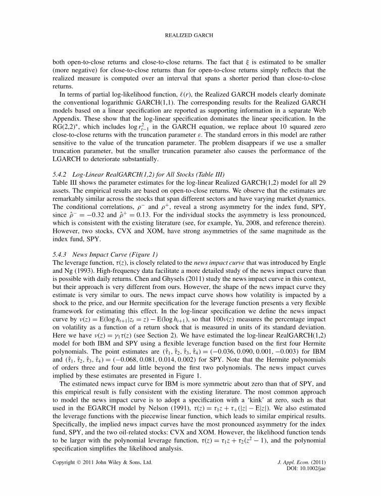
5.4.3 News Impact Curve (Figure 1)The leverage function, ��z�, is closely related to the news impact curve that was introduced by Engleand Ng (1993). High-frequency data facilitate a more detailed study of the news impact curve thanis possible with daily returns. Chen and Ghysels (2011) study the news impact curve in this context,but their approach is very different from ours. However, the shape of the news impact curve theyestimate is very similar to ours. The news impact curve shows how volatility is impacted by ashock to the price, and our Hermite specification for the leverage function presents a very flexibleframework for estimating this effect. In the log-linear specification we define the news impactcurve by ��z� D E�log htC1jzt D z�� E�log htC1�, so that 100��z� measures the percentage impacton volatility as a function of a return shock that is measured in units of its standard deviation.Here we have ��z� D �1��z� (see Section 2). We have estimated the log-linear RealGARCH(1,2)model for both IBM and SPY using a flexible leverage function based on the first four Hermitepolynomials. The point estimates are �O�1, O�2, O�3, O�4� D ��0.036, 0.090, 0.001,�0.003� for IBMand �O�1, O�2, O�3, O�4� D ��0.068, 0.081, 0.014, 0.002� for SPY. Note that the Hermite polynomialsof orders three and four add little beyond the first two polynomials. The news impact curvesimplied by these estimates are presented in Figure 1.
The estimated news impact curve for IBM is more symmetric about zero than that of SPY, andthis empirical result is fully consistent with the existing literature. The most common approachto model the news impact curve is to adopt a specification with a ‘kink’ at zero, such as thatused in the EGARCH model by Nelson (1991), ��z� D �1z C �C�jzj � Ejzj�. We also estimatedthe leverage functions with the piecewise linear function, which leads to similar empirical results.Specifically, the implied news impact curves have the most pronounced asymmetry for the indexfund, SPY, and the two oil-related stocks: CVX and XOM. However, the likelihood function tendsto be larger with the polynomial leverage function, ��z� D �1z C �2�z2 � 1�, and the polynomialspecification simplifies the likelihood analysis.
Copyright 2011 John Wiley & Sons, Ltd. J. Appl. Econ. (2011)DOI: 10.1002/jae

P. R. HANSEN, Z. HUANG AND H. H. SHEK
Table III. Estimates for the log-linear Realized GARCH�1, 2� model
ω ˇ �1 �2 � ϕ �u �1 �2 ��r� ��r, x� � �� �C
AA 0.03 0.77 0.33 �0.14 �0.07 1.15 0.40 �0.04 0.09 �2776.4 �3519.9 0.98 �0.08 �0.32 0.24AIG 0.02 0.74 0.45 �0.21 �0.06 1.02 0.45 �0.02 0.04 �2403.1 �3317.2 0.98 �0.06 �0.17 0.08AXP 0.05 0.70 0.38 �0.12 �0.16 1.08 0.43 �0.02 0.10 �2371.1 �3217.9 0.99 �0.05 �0.30 0.25BA 0.02 0.82 0.31 �0.17 �0.13 1.22 0.39 �0.03 0.09 �2536.0 �3260.0 0.99 �0.09 �0.36 0.26BAC 0.00 0.78 0.51 �0.29 0.00 0.99 0.42 �0.04 0.08 �2016.9 �2823.4 0.99 �0.09 �0.31 0.21C �0.02 0.74 0.45 �0.19 0.09 0.99 0.39 �0.03 0.09 �2260.5 �2974.0 0.99 �0.07 �0.31 0.24CAT 0.03 0.82 0.37 �0.22 �0.14 1.07 0.38 �0.03 0.09 �2621.1 �3279.4 0.99 �0.08 �0.32 0.27CVX 0.03 0.71 0.33 �0.14 �0.09 1.32 0.39 �0.08 0.08 �2319.1 �3021.8 0.97 �0.19 �0.35 0.14DD �0.01 0.77 0.37 �0.17 0.08 1.08 0.40 �0.05 0.08 �2301.2 �3067.3 0.98 �0.13 �0.35 0.20DIS 0.01 0.85 0.39 �0.25 �0.05 1.10 0.41 �0.04 0.09 �2518.5 �3289.6 1.00 �0.09 �0.35 0.22GE 0.00 0.81 0.38 �0.19 0.01 0.98 0.41 �0.01 0.08 �2197.8 �2988.7 0.99 �0.02 �0.26 0.25GM 0.06 0.84 0.39 �0.24 �0.32 1.02 0.47 �0.01 0.12 �2987.9 �3967.3 0.99 �0.01 �0.33 0.31HD 0.01 0.79 0.39 �0.20 0.00 1.01 0.41 �0.05 0.09 �2538.4 �3318.4 0.99 �0.13 �0.37 0.20IBM 0.00 0.74 0.41 �0.15 0.01 0.94 0.39 �0.04 0.08 �2192.6 �2896.7 0.98 �0.09 �0.32 0.24INTC 0.02 0.87 0.46 �0.33 �0.11 1.03 0.36 �0.02 0.07 �2869.1 �3481.1 1.00 �0.05 �0.24 0.22JNJ �0.03 0.80 0.38 �0.19 0.13 1.04 0.44 0.02 0.10 �1874.8 �2777.3 0.99 0.04 �0.25 0.30JPM 0.01 0.81 0.49 �0.30 �0.02 0.98 0.42 �0.04 0.09 �2463.0 �3276.8 0.99 �0.10 �0.30 0.22KO �0.05 0.76 0.45 �0.21 0.19 0.93 0.38 �0.02 0.07 �1886.7 �2573.6 0.99 �0.06 �0.28 0.19MCD 0.00 0.88 0.37 �0.25 �0.01 0.98 0.45 �0.05 0.11 �2461.8 �3371.9 0.99 �0.09 �0.35 0.26MMM 0.00 0.77 0.43 �0.23 0.02 0.98 0.41 �0.02 0.07 �2140.3 �2944.8 0.97 �0.04 �0.23 0.21MRK 0.03 0.84 0.33 �0.21 �0.19 1.23 0.47 0.01 0.07 �2479.2 �3478.5 0.98 0.04 �0.13 0.18MSFT �0.01 0.79 0.44 �0.22 0.08 0.92 0.38 �0.03 0.08 �2330.7 �3021.1 0.99 �0.08 �0.31 0.24PG �0.04 0.78 0.43 �0.25 0.18 1.04 0.41 �0.05 0.08 �1850.7 �2646.6 0.98 �0.14 �0.32 0.14T 0.00 0.86 0.53 �0.38 0.01 0.86 0.46 �0.03 0.10 �2560.4 �3512.7 0.99 �0.07 �0.32 0.25UTX �0.01 0.80 0.45 �0.24 0.06 0.88 0.40 �0.01 0.10 �2302.4 �3059.2 0.99 �0.05 �0.34 0.29VZ �0.01 0.79 0.40 �0.20 0.07 1.01 0.43 �0.03 0.09 �2343.4 �3196.7 0.99 �0.08 �0.31 0.23WMT �0.02 0.80 0.37 �0.19 0.12 1.04 0.39 �0.01 0.09 �2164.9 �2893.6 0.99 �0.02 �0.29 0.30XOM 0.03 0.71 0.34 �0.12 �0.10 1.26 0.38 �0.08 0.08 �2334.7 �2994.1 0.98 �0.20 �0.37 0.15SPY 0.04 0.70 0.45 �0.18 �0.18 1.04 0.38 �0.07 0.07 �1710.3 �2388.8 0.99 �0.17 �0.32 0.13Average 0.01 0.79 0.41 �0.21 �0.02 1.04 0.41 �0.03 0.09 0.99 �0.08 �0.30 0.22
5.4.4 In-Sample and Out-of-Sample Log-Likelihood ResultsTable IV presents likelihood ratio statistics using open-to-close returns. The inference we drawfrom these statistics is that RealGARCH(1,2) is generally a good model. Moreover, the leveragefunction is highly significant, whereas ˛ is insignificant.
The statistics in panel A are conventional likelihood ratio statistics:
LRi D 2f�RG�2,2�Ł�r, x�� �i�r, x�g, i D 1, . . . , 5
where each of the five smaller models are benchmarked against the largest model. The largest modelis the log-linear RealGARCH(2,2) model, which includes the squared returns in the GARCHequation (in addition to the realized measure). In the QMLE framework the limit distributionof likelihood ratio statistic, LRi, is usually given as a weighted sum of �2-distributed randomvariables. Thus comparing the LRi with the usual critical value of a �2-distribution is onlyindicative of significance. The LR statistics in the column labeled ‘(2,2)’ are small in most cases,so there is little evidence that ˛ is significant. This is consistent with the existing literature, sincesquared returns are typically found to be insignificant once a realized measure is included inthe GARCH equation. The LR statistics in column ‘(2,2)†’ are well over 100 in all cases. Thisshows that the leverage function, ��zt�, is highly significant. Similarly, the LR statistics showthat the hypothesis, ˇ2 D �2 D 0, is rejected in most cases. Therefore the empirical evidence doesnot support a simplification of the model to the RealGARCH(1,1). The results for the two sub-hypotheses ˇ2 D 0 and �2 D 0 are less conclusive. The likelihood ratio statistics for the hypothesis
Copyright 2011 John Wiley & Sons, Ltd. J. Appl. Econ. (2011)DOI: 10.1002/jae

REALIZED GARCH
News Impact Curve
15%
IBMSPY
10%
5%
0%-2.0 -1.5 -1.0 -0.5 0.0 0.5 1.0 1.5 2.0
-5%
Figure 1. News impact curve for IBM and SPY
ˇ2 D 0 (which is given as the difference between the statistics in columns ‘(1,2)’ and ‘(2,2)’) are onaverage 5.7 D 9.6 � 3.9. In a correctly specified model, this would be borderline significant. TheLR statistics for the hypothesis �2 D 0 tend to be larger with an average value of 16.6 D 20.5 � 3.9.Thus the empirical evidence favors the RealGARCH(1,2) model over the RealGARCH(2,1) model.
The statistics in panel B are out-of-sample likelihood ratio statistics, defined by√nm f�RG�2,2�
�r, x�� �j�r, x�g, where n and m denote the sample sizes, in-sample and out-of-sample, respec-tively. The in-sample estimates are simply plugged into the out-of-sample log-likelihood function.The asymptotic distribution of the out-of-sample LR statistic is non-standard. However, in a nestedcomparison where the larger model has k additional parameters (which are all zero in population),it can be shown that√
n
mf�i�r, x�� �j�r, x�g d!Z0
1Z2, as m, n ! 1 with m/n ! 0
where Z1 and Z2 are independent Zi ∼ Nk�0, I�, and is a diagonal matrix with eigenvalues fromI�1J (see Hansen, 2009). For correctly specified models � D I� the (two-sided) critical values canbe inferred from the distribution of jZ0
1Z2j. For k D 1 the 5% and 1% critical values are 2.25 and3.67, respectively, and for two degrees of freedom (k D 2), these are 3.05 and 4.83, respectively.Although our model is likely to be misspecified to some degree, we will later argue that the log-linear Gaussian specification is not very misspecified. Therefore we will take these critical valuesas reasonable approximations. Compared to these critical values we find, on average, significantevidence in favor of a model with more lags than RealGARCH(1,1). The statistical evidencein favor of a leverage function is again very strong. Adding the ARCH parameter, ˛, will (onaverage) result in a worse out-of-sample log-likelihood. On average, we have a tie between thethree models: RealGARCH(1,2), RealGARCH(2,1), and RealGARCH(2,2).
Copyright 2011 John Wiley & Sons, Ltd. J. Appl. Econ. (2011)DOI: 10.1002/jae

P. R. HANSEN, Z. HUANG AND H. H. SHEK
Tabl
eIV
.In
-sam
ple
and
out-
of-s
ampl
elik
elih
ood
ratio
stat
istic
s
Pane
lA
:In
-sam
ple
likel
ihoo
dra
tioPa
nel
B:
Out
-of-
sam
ple
likel
ihoo
dra
tioPa
nel
C:
Out
-of-
sam
ple
part
ial
likel
ihoo
dra
tio
(1,1
)(1
,2)
(2,1
)(2
,2)
(2,2
)†(2
,2)Ł
(1,1
)(1
,2)
(2,1
)(2
,2)
(2,2
)†(2
,2)Ł
G11
(1,1
)(1
,2)
(2,1
)(2
,2)
(2,2
)†(2
,2)Ł
AA
24.0
8.3
11.7
3.9
187.
40
6.9
4.5
6.4
021
.90.
14.
63.
31.
42.
60.
00.
60.
7A
IG43
.815
.220
.614
.220
1.2
015
.7�0
.26.
00
25.5
12.5
56.1
9.3
5.9
7.4
6.0
0.0
7.2
AX
P30
.525
.026
.00.
019
7.0
01.
22.
71.
50
13.3
0.2
24.0
0.0
0.3
0.1
1.3
1.7
1.4
BA
34.8
6.0
18.8
0.0
197.
10
�1.4
0.4
�2.6
024
.50.
01.
10.
61.
81.
70.
00.
30.
0B
AC
46.3
5.9
20.5
5.1
198.
80
8.0
�0.7
�0.3
056
.5�2
.814
7.9
4.1
0.6
0.0
1.5
19.7
0.9
C26
.89.
516
.06.
322
8.4
01.
3�2
.7�2
.50
�0.1
�7.2
26.9
0.3
0.9
0.5
1.1
0.0
0.4
CA
T39
.82.
313
.81.
622
7.3
01.
7�1
.0�4
.20
9.0
2.2
47.3
0.1
0.8
0.0
1.0
1.6
1.5
CV
X17
.70.
13.
50.
019
4.6
05.
30.
02.
20
20.8
�0.1
30.1
0.6
0.3
0.2
0.3
0.0
0.3
DD
31.1
10.8
15.9
6.1
167.
00
4.6
4.1
3.0
0�7
.16.
919
.21.
21.
51.
51.
21.
40.
0D
IS57
.712
.633
.10.
021
3.7
04.
84.
83.
70
24.3
0.0
35.4
0.0
2.0
1.4
0.8
1.1
0.8
GE
37.7
12.6
20.2
12.2
200.
30
14.1
0.6
5.9
09.
30.
641
.60.
90.
00.
60.
00.
30.
7G
M62
.718
.839
.918
.431
9.9
017
.0�0
.26.
80
7.2
14.6
57.5
1.4
0.0
0.2
0.0
0.3
0.9
HD
29.8
4.0
14.4
2.0
201.
30
2.2
�1.0
�1.0
028
.90.
545
.50.
90.
00.
10.
22.
10.
4IB
M28
.516
.220
.21.
017
6.7
03.
3�0
.11.
00
25.0
�0.2
12.0
0.4
0.5
0.7
0.1
0.3
0.0
INT
C75
.913
.947
.89.
713
0.8
00.
90.
1�3
.40
36.8
19.1
133.
11.
70.
52.
00.
00.
11.
8JN
J34
.61.
34.
80.
123
5.4
07.
1�0
.82.
00
30.7
0.2
21.8
0.4
0.0
0.1
0.1
0.1
0.0
JPM
50.7
3.5
23.6
1.9
213.
50
0.3
�2.5
�5.4
0�3
.6�0
.634
.90.
01.
30.
11.
62.
01.
6K
O39
.722
.028
.30.
018
6.1
02.
1�2
.8�1
.00
22.6
0.0
5.6
0.4
0.6
0.0
0.5
0.9
0.5
MC
D54
.82.
926
.10.
827
8.6
0�1
3.0
�0.6
�9.3
047
.41.
46.
80.
01.
50.
21.
82.
01.
7M
MM
32.0
6.7
20.4
0.1
183.
50
�2.4
�0.2
�2.8
024
.5�0
.114
.50.
01.
90.
91.
41.
01.
4M
RK
64.6
12.0
10.6
2.9
309.
00
�3.4
�2.5
�1.2
032
.40.
411
.80.
01.
61.
71.
92.
41.
8M
SFT
37.3
11.5
20.5
10.2
186.
10
8.3
4.2
7.1
017
.04.
137
.10.
10.
50.
40.
00.
20.
1PG
36.5
3.0
12.3
2.9
160.
40
�1.3
0.3
�0.4
035
.01.
024
.80.
01.
40.
61.
31.
51.
7T
69.8
4.8
39.0
0.0
198.
30
19.7
�0.3
13.5
035
.1�0
.219
.22.
80.
22.
60.
01.
70.
0U
TX
39.6
21.6
29.0
0.0
223.
70
5.8
�2.0
1.2
033
.1�0
.412
.31.
40.
20.
90.
20.
00.
1V
Z31
.54.
313
.20.
518
8.7
015
.03.
211
.10
16.6
�1.3
8.7
3.5
0.7
2.8
0.3
0.0
0.1
WM
T36
.212
.023
.08.
319
0.0
0�7
.2�3
.8�7
.90
28.7
9.4
30.5
0.0
0.6
0.0
1.3
1.4
2.6
XO
M14
.71.
14.
30.
923
4.0
05.
7�0
.11.
00
27.9
0.6
21.6
0.0
0.5
0.3
0.5
0.5
0.5
SPY
25.3
11.6
17.9
4.2
225.
60
6.3
�1.2
1.9
024
.41.
440
.80.
80.
60.
70.
02.
51.
3A
vera
ge39
.89.
620
.53.
920
8.8
04.
40.
11.
10
23.0
2.1
33.5
1.2
1.0
1.0
0.8
1.6
1.0
Copyright 2011 John Wiley & Sons, Ltd. J. Appl. Econ. (2011)DOI: 10.1002/jae

REALIZED GARCH
In panel C, we report partial out-of-sample likelihood ratio statistics that are defined by2fmaxi �i�rjx�� �j�rjx�g. These LR statistics are based on the partial likelihood for returns, whichenables us to compare the empirical fit to the conventional LGARCH. Again we see that theRealized GARCH models strongly dominate the LGARCH(1,1) model. This is impressive becausethe Realized GARCH models are not seeking to maximize the partial likelihood, as is the objectivefor the LGARCH model.4
5.5. A Comparison of the Linear and Log-Linear Specifications
One of the reasons we prefer the log-linear Gaussian specification over the linear Gaussian spec-ification is that the former is much less at odds with the data. The log-linear specification resultsin far less heteroskedasticity, as is evident from Figure 2. The left-hand panel is a scatter plot ofxt against Oht, (for the linear RealGARCH(1,2) model) and the right-hand panel is a scatter plot oflog xt against log Oht (for the log-linear RealGARCH(1,2) model). The two models produce verysimilar value for ht; however, there is obviously a very pronounced degree of heteroskedasticity inthe linear models. The linear model may be improved by modifying the leverage function, but ourpoint is that the simple measurement equation does a good job within the log-linear specification.Homoskedastic errors are not essential for the QMLEs but heteroskedasticity causes the QMLE tobe inefficient. Moreover, misspecification causes the likelihood ratio statistic to have an asymptoticdistribution that is a weighted sum of �2
�1�-distributed random variables, rather than a pure sum ofsuch. Comparing likelihood ratio statistics with critical values to a standard �2-distribution, as anapproximation, becomes dubious when the model is highly misspecified.
Figure 3 presents additional evidence in favor of log-linear specification, and shows that theleverage function is critical for the validity of the assumed independence between zt and ut. Thefigure has four scatter plots of the residuals, fOzt, OutgntD1, where each scatter plot corresponds toa particular specification. The upper panels in Figure 3 are for the linear specification and thetwo lower panels are for the log-linear specification. Left panels are based on residuals obtainedwithout a leverage function (i.e. ��z� D 0), and those on the right are the residuals obtained witha quadratic specification for ��z�. Ideally the scatter plot would look like one of two independentGaussian distributed random variables. The upper panels are clearly at odds with this, which
0
2
4
6
8
10
12
14
0 2 4 6 8 10 12
xt
ht
Linear Model: x against h
-4
-3
-2
-1
0
1
2
3
-3 -2 -1 0 1 2 3
log(xt)
log(ht)
Log-Linear Model: log(x) against log(h)
Figure 2. Heteroskedasticity in measurement equation
4 The asymptotic distribution of these statistics is very non-standard (and generally unknown) because we are comparinga model that maximizes the partial likelihood (the LGARCH(1,1) model) with models that maximize a joint likelihood(the Realized GARCH models).
Copyright 2011 John Wiley & Sons, Ltd. J. Appl. Econ. (2011)DOI: 10.1002/jae

P. R. HANSEN, Z. HUANG AND H. H. SHEK
u
z
Linear specification without leverage functionu
z
Linear specification with quadratic leverage function
u
z
Log-linear specification without leverage functionu
z
Log-linear specification with quadratic leverage function
Figure 3. Scatter plots of the residuals, �Ozt, Out�, obtained with four different RealGARCH(1,2) models.The upper panels are for the linear specification and the lower panels are for the log-linear specification.The left-hand panels are for models without a leverage function and the right-hand panels are with aquadratic leverage function. The log-linear specification with the leverage function is clearly best suitedfor the Gaussian structure of the quasi log-likelihood function. This figure is available in color online atwileyonlinelibrary.com/journal/jae
confirms that the linear specification is highly misspecified. The lower-left panel is the log-linearspecification without a leverage function, and it clearly reveals unmodeled dependence between ztand ut. The log-linear model with quadratic leverage function (lower-right panel) offers a muchbetter agreement with the underlying assumptions.
The fact that the log-linear model is far less misspecified than the linear model can alsobe illustrated by comparing robust and non-robust standard errors. In Table V we have com-puted standard errors using those of the two information matrices (the diagonal elements ofI�1 and J�1) and the robust standard errors computed from the diagonal of I�1JI�1. In acorrectly specified model these standard errors should be in agreement. This is obviously notthe case for the linear specification, whereas there is better agreement with the log-linearspecification.
Copyright 2011 John Wiley & Sons, Ltd. J. Appl. Econ. (2011)DOI: 10.1002/jae

REALIZED GARCH
Table V. Conventional and robust standard errors computed for Realized GARCH(1,2) model with a quadraticleverage function. The data are open–close SPY returns
Standard errors for RealGARCH(1,2) Model
Linear model Log-linear model
I�1 J�1 I�1JI�1 I�1 J�1 I�1JI�1
ω 0.007 0.004 0.019 0.015 0.015 0.016ˇ 0.034 0.017 0.125 0.040 0.031 0.053�1 0.053 0.040 0.133 0.030 0.025 0.040�2 0.054 0.032 0.177 0.046 0.036 0.062� 0.038 0.037 0.096 0.044 0.042 0.051ϕ 0.080 0.064 0.212 0.044 0.033 0.069�u 0.009 0.002 0.054 0.005 0.005 0.006�1 0.013 0.014 0.016 0.010 0.011 0.011�2 0.008 0.013 0.011 0.006 0.008 0.006
6. MOMENTS, FORECASTING, AND INSIGHT ABOUT THE REALIZED MEASURE
In this section we discuss the skewness and kurtosis (for cumulative returns) that the RealizedGARCH model can generate for realistic values of the parameters and we discuss issues relatedto multi-period forecasting in the Realized GARCH context.
6.1. Properties of Cumulative Returns: Skewness and Kurtosis
We consider the skewness and kurtosis for returns generated by a Realized GARCH model. Someanalytical results in closed form can be derived for the linear Realized GARCH model. Theseresults are given as supporting information in a separate Web Appendix. Here we will focus onthe log-linear Realized GARCH model. We have the following results for the kurtosis of a singleperiod return.
Proposition 1. Consider the log-linear RealGARCH(1,1) model and define D ˇ C ϕ� and D ω C ϕ�, so that
log ht D log ht�1 C C �wt�1, where wt D �1zt C �2�z2t � 1�C ut
with zt ∼ i.i.d.N�0, 1� and ut ∼ i.i.d.N�0, �2u �. The kurtosis of the return rt D p
htzt is given by
E�r4t �
E�r2t �
2 D 3
( 1∏iD0
1 � 2i��2√1 � 4i��2
)exp
{ 1∑iD0
2i�2�21
1 � 6i��2 C 82i�2�22
}exp
{�2�2
u
1 � 2
}�8�
There does not appear to be a way to further simplify expression (8); however, when ��2 is
small, as we found it to be empirically, we have the approximationE�r4
t �E�r2
t �2 ' 3 exp
{�2�2
2� logC�2��2
1 C �2u �
1 � 2
}(see the Web Appendix for details). The skewness for single period returns is non-
zero, if and only if the Studentized return, zt, has non-zero skewness. This follows directly fromthe identity rt D p
htzt, and the assumption that zt??ht, which shows that E�rdt � D E�hd/2t zdt � DEfE�hd/2t zdt jFt�1�g D E�hd/2t �E�zdt �, and in particular that E�r3
t � D E�h3/2t �E�z3
t �. Thus a symmetric
Copyright 2011 John Wiley & Sons, Ltd. J. Appl. Econ. (2011)DOI: 10.1002/jae
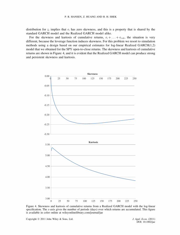
P. R. HANSEN, Z. HUANG AND H. H. SHEK
distribution for zt implies that rt has zero skewness, and this is a property that is shared by thestandard GARCH model and the Realized GARCH model alike.
For the skewness and kurtosis of cumulative returns, rt C . . .C rtCk , the situation is verydifferent, because the leverage function induces skewness. For this problem we resort to simulationmethods using a design based on our empirical estimates for log-linear Realized GARCH(1,2)model that we obtained for the SPY open-to-close returns. The skewness and kurtosis of cumulativereturns are shown in Figure 4, and it is evident that the Realized GARCH model can produce strongand persistent skewness and kurtosis.
-0.15
-0.10
-0.05
0.000 25 50 75 100 125 150 175 200 225 250
Skewness
-0.30
-0.25
-0.20
4.50
5.00
5.50Kurtosis
3.00
3.50
4.00
0 25 50 75 100 125 150 175 200 225 250
Figure 4. Skewness and kurtosis of cumulative returns from a Realized GARCH model with the log-linearspecification. The x-axis gives the number of periods (days) over which returns are accumulated. This figureis available in color online at wileyonlinelibrary.com/journal/jae
Copyright 2011 John Wiley & Sons, Ltd. J. Appl. Econ. (2011)DOI: 10.1002/jae
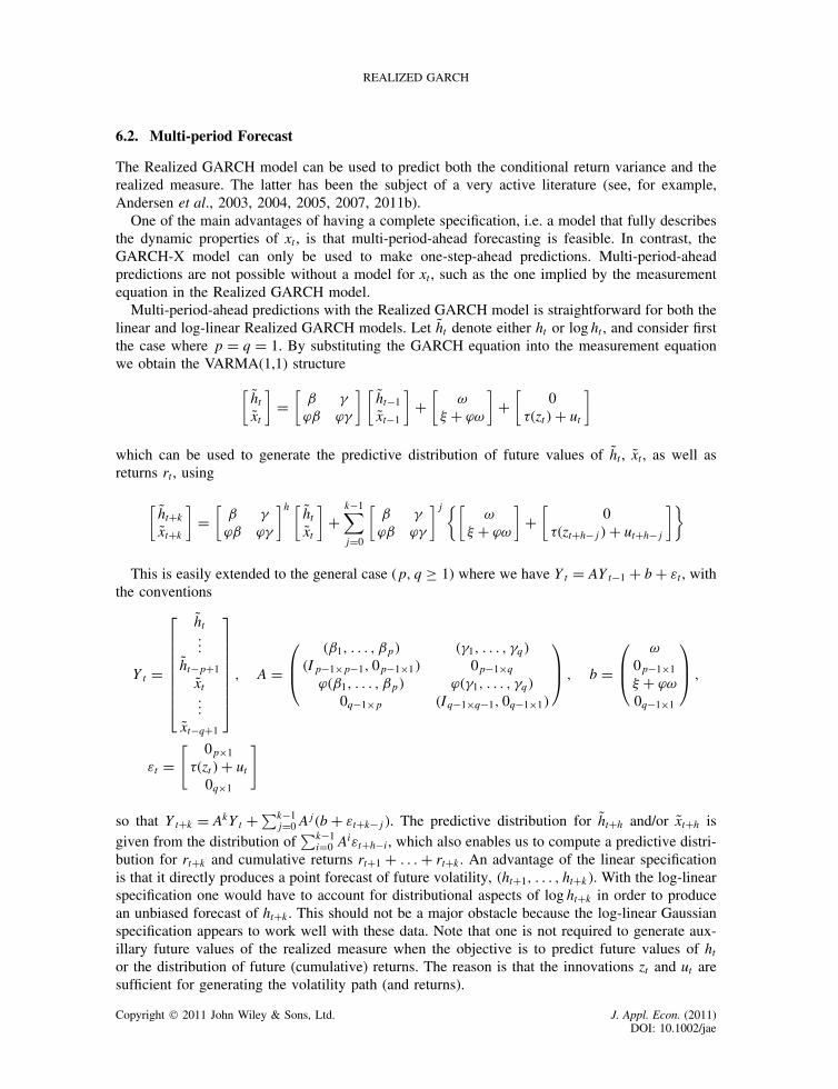
REALIZED GARCH
6.2. Multi-period Forecast
The Realized GARCH model can be used to predict both the conditional return variance and therealized measure. The latter has been the subject of a very active literature (see, for example,Andersen et al., 2003, 2004, 2005, 2007, 2011b).
One of the main advantages of having a complete specification, i.e. a model that fully describesthe dynamic properties of xt, is that multi-period-ahead forecasting is feasible. In contrast, theGARCH-X model can only be used to make one-step-ahead predictions. Multi-period-aheadpredictions are not possible without a model for xt, such as the one implied by the measurementequation in the Realized GARCH model.
Multi-period-ahead predictions with the Realized GARCH model is straightforward for both thelinear and log-linear Realized GARCH models. Let Qht denote either ht or log ht, and consider firstthe case where p D q D 1. By substituting the GARCH equation into the measurement equationwe obtain the VARMA(1,1) structure[ Qht
Qxt]
D[ˇ �ϕˇ ϕ�
] [ Qht�1
Qxt�1
]C[
ω� C ϕω
]C[
0��zt�C ut
]
which can be used to generate the predictive distribution of future values of Qht, Qxt, as well asreturns rt, using
[ QhtCkQxtCk
]D[ˇ �ϕˇ ϕ�
]h [ QhtQxt]
Ck�1∑jD0
[ˇ �ϕˇ ϕ�
]j {[ω
� C ϕω
]C[
0��ztCh�j�C utCh�j
]}
This is easily extended to the general case (p, q ½ 1) where we have Yt D AYt�1 C bC εt, withthe conventions
Yt D
Qht...
Qht�pC1
Qxt...
Qxt�qC1
, A D
�ˇ1, . . . , ˇp� ��1, . . . , �q��Ip�1ðp�1, 0p�1ð1� 0p�1ðqϕ�ˇ1, . . . , ˇp� ϕ��1, . . . , �q�
0q�1ðp �Iq�1ðq�1, 0q�1ð1�
, b D
ω0p�1ð1
� C ϕω0q�1ð1
,
εt D[ 0pð1
��zt�C ut0qð1
]
so that YtCk D AkYt C∑k�1jD0 A
j�b C εtCk�j�. The predictive distribution for QhtCh and/or QxtCh isgiven from the distribution of
∑k�1iD0 A
iεtCh�i, which also enables us to compute a predictive distri-bution for rtCk and cumulative returns rtC1 C . . .C rtCk . An advantage of the linear specificationis that it directly produces a point forecast of future volatility, �htC1, . . . , htCk�. With the log-linearspecification one would have to account for distributional aspects of log htCk in order to producean unbiased forecast of htCk . This should not be a major obstacle because the log-linear Gaussianspecification appears to work well with these data. Note that one is not required to generate aux-illary future values of the realized measure when the objective is to predict future values of htor the distribution of future (cumulative) returns. The reason is that the innovations zt and ut aresufficient for generating the volatility path (and returns).
Copyright 2011 John Wiley & Sons, Ltd. J. Appl. Econ. (2011)DOI: 10.1002/jae

P. R. HANSEN, Z. HUANG AND H. H. SHEK
7. CONCLUSION
In this paper we have proposed a complete model for returns and realized measures of volatility,xt, where the latter is tied directly to the conditional volatility ht. We have demonstrated that themodel is straightforward to estimate and offers a substantial improvement in the empirical fit,relative to standard GARCH models based on daily returns only. The model is informative aboutrealized measurement, such as its accuracy.
Our empirical analysis can be extended in a number of ways. For instance, inclusion of ajump-robust realized measure would be an interesting extension, because Andersen et al. (2007)have shown that the predictability in volatility is largely driven by the continuous componentof volatility. Moreover, Bollerslev et al. (2009) have found that the leverage effect primarily actsthrough the continuous volatility component. Another possible extension is to introduce a bivariatemodel of open-to-close and close-to-open returns as an alternative to modeling close-to-closereturns (see Andersen et al., 2011a).
The Realized GARCH framework is naturally extended to a multi-factor structure, e.g. withm realized measures and k latent volatility variables, the Realized GARCH model discussed inthis paper corresponds to the case k D 1, whereas the MEM framework corresponds to the casem D k. Such a hybrid framework would enable us to conduct an inference about the number oflatent factors, k. We could, in particular, test the one-factor structure used in this paper against themulti-factor structure implied by MEM.
ACKNOWLEDGEMENTS
We thank Tim Bollerslev, Giampiero Gallo, Asger Lunde, and seminar participants at HumboldtUniversity, the Einaudi Institute, the 2009 Stanford Institute for Theoretical Economics, and theVolatility Institute at New York University Stern School of Business for valuable comments.
REFERENCES
Andersen TG, Bollerslev T. 1998. Answering the skeptics: yes, standard volatility models do provide accurateforecasts. International Economic Review 39(4): 885–905.
Andersen TG, Bollerslev T, Diebold FX, Labys P. 2001. The distribution of exchange rate volatility. Journalof the American Statistical Association 96(453): 42–55 (correction published 2003, Vol. 98, p. 501).
Andersen TG, Bollerslev T, Diebold FX, Labys P. 2003. Modeling and forecasting realized volatility.Econometrica 71(2): 579–625.
Andersen TG, Bollerslev T, Meddahi N. 2004. Analytic evaluation of volatility forecasts. InternationalEconomic Review 45: 1079–1110.
Andersen TG, Bollerslev T, Meddahi N. 2005. Correcting the errors: volatility forecast evaluation usinghigh-frequency data and realized volatilities. Econometrica 73: 279–296.
Andersen T, Bollerslev T, Diebold FX. 2007. Roughing it up: including jump components in the measure-ment, modeling and forecasting of return volatility. Review of Economics and Statistics 89: 701–720.
Andersen T, Dobrev D, Schaumburg E. 2008. Duration-based volatility estimation. Working paper Depart-ment of Finance, Kellogg School, Northwestern University.
Andersen TG, Bollerslev T, Huang X. 2011a. A reduced form framework for modeling volatility ofspeculative prices based on realized variation measures. Journal of Econometrics 160: 176–189.
Andersen TG, Bollerslev T, Meddahi N. 2011b. Realized volatility forecasting and market microstructurenoise. Journal of Econometrics 160: 220–234.
Barndorff-Nielsen OE, Shephard N. 2002. Econometric analysis of realised volatility and its use in estimatingstochastic volatility models. Journal of the Royal Statistical Society B 64: 253–280.
Barndorff-Nielsen OE, Shephard N. 2004. Power and bipower variation with stochastic volatility and jumps(with discussion). Journal of Financial Econometrics 2: 1–48.
Copyright 2011 John Wiley & Sons, Ltd. J. Appl. Econ. (2011)DOI: 10.1002/jae

REALIZED GARCH
Barndorff-Nielsen OE, Shephard N. 2007. Variation, jumps and high frequency data in financial econo-metrics. In Advances in Economics and Econometrics: Theory and Applications. Ninth World Congress,Econometric Society Monographs. Cambridge University Press: Cambridge, UK; 328–372.
Barndorff-Nielsen OE, Hansen PR, Lunde A, Shephard N. 2008. Designing realised kernels to measure theex-post variation of equity prices in the presence of noise. Econometrica 76: 1481–536.
Barndorff-Nielsen OE, Hansen PR, Lunde A, Shephard N. 2009a. Realised kernels in practice: trades andquotes. Econometrics Journal 12: 1–33.
Barndorff-Nielsen OE, Kinnebrock S, Shephard N. 2009b. Measuring downside risk: realised semivariance.In Volatility and Time Series Econometrics: Essays in Honor of Robert Engle, Watson MW, Bollerslev T,Russell J (eds). Oxford University Press: Oxford; 117–137.
Barndorff-Nielsen OE, Hansen PR, Lunde A, Shephard N. 2010. Multivariate realised kernels: consistentpositive semi-definite estimators of the covariation of equity prices with noise and non-synchronous trading.Journal of Econometrics , DOI: 10.1016/j.jeconom.2010.07.009.
Bollerslev T. 1986. Generalized autoregressive heteroskedasticity. Journal of Econometrics 31: 307–327.Bollerslev T. 2009. Glossary to ARCH (GARCH). In Volatility and Time Series Econometrics: Essays in
Honour of Robert F. Engle, Bollerslev T, Russell JR, Watson M (eds). Oxford University Press: Oxford,UK; 137–164.
Bollerslev T, Wooldridge JM. 1992. Quasi-maximum likelihood estimation and inference in dynamic modelswith time-varying covariance. Econometric Reviews 11: 143–172.
Bollerslev T, Kretschmer U, Pigorsch C, Tauchen G. 2009. A discrete-time model for daily S&P500 returnsand realized variations: jumps and leverage effects. Journal of Econometrics 150: 151–66.
Brownless CT, Gallo GM. 2010. Comparison of volatility measures: a risk management perspective. Journalof Financial Econometrics 8: 29–56.
Carrasco M, Chen X. 2002. Mixing and moment properties of various GARCH and stochastic volatilitymodels. Econometric Theory 18: 17–39.
Chen X, Ghysels E, Wang F. 2009. The HYBRID GARCH class of models. Working paper University ofNorth Carolina at Chapel Hill.
Christoffersen P, Feunou B, Jacobs K, Meddahi N. 2010. The economic value of realized volatility. Workingpaper McGill University.
Cipollini F, Engle RF, Gallo GM. 2009. A model for multivariate non-negative valued processes in financialeconometrics. Working paper Available at SSRN: http://ssrn.com/abstract=1333869.
Dobrev D, Szerszen P. 2010. The information content of high-frequency data for estimating equity returnmodels and forecasting risk. Working paper Board of Governors of the Federal Reserve System,International Finance Discussion Papers,nr. 1005.
Engle RF. 1982. Autoregressive conditional heteroskedasticity with estimates of the variance of U.K.inflation. Econometrica 45: 987–1007.
Engle RF. 2002. New frontiers of ARCH models. Journal of Applied Econometrics 17: 425–446.Engle RF, Gallo G. 2006. A multiple indicators model for volatility using intra-daily data. Journal of
Econometrics 131: 3–27.Engle RF, Ng V. 1993. Measuring and testing the impact of news on volatility. Journal of Finance 48:
1747–1778.Engle RF, Lilien DV, Robins RP. 1987. Estimating time varying risk premia in the term structure: the
ARCH-M model. Econometrica 55: 391–407.Forsberg L, Bollerslev T. 2002. Bridging the gap between the distribution of realized (ECU) volatility
and ARCH modeling (of the EURO): the GARCH-NIG model. Journal of Applied Econometrics 17(5):535–548.
Geweke J. 1986. Modelling persistence in conditional variances: a comment. Econometric Reviews 5: 57–61.Chen X, Ghysels E. 2011. News–-good or bad–-and its impact on volatility predictions over multiple
horizons. Review of Financial Studies 24: 46–81.Hansen PR. 2009. In-sample fit and out-of-sample fit: their joint distribution and its implications for model
selection. Working paper Department of Economics, Stanford University.Hansen PR, Horel G. 2009. Quadratic variation by Markov chains. Working paper. Department of Economics,
Stanford University.Jensen ST, Rahbek A. 2004a. Asymptotic inference for nonstationary GARCH. Econometric Theory 20:
1203–1226.Jensen ST, Rahbek A. 2004b. Asymptotic normality of the QMLE estimator of ARCH in the nonstationary
case. Econometrica 72: 641–646.Lee S, Hansen BE. 1994. Asymptotic theory for the GARCH(1,1) quasi-maximum likelihood estimator.
Econometric Theory 10: 29–52.
Copyright 2011 John Wiley & Sons, Ltd. J. Appl. Econ. (2011)DOI: 10.1002/jae

P. R. HANSEN, Z. HUANG AND H. H. SHEK
Lumsdaine RL. 1996. Consistency and asymptotic normality of the quasi-maximum likelihood estimator inIGARCH(1,1) and covariance stationary GARCH(1,1) models. Econometrica 10: 29–52.
Meddahi N. 2003. ARMA representation of integrated and realized variances. Econometrics Journal 6:335–356.
Milhøj A. 1987. A multiplicative parameterization of ARCH models. Technical report, Department ofStatistics, University of Copenhagen.
Nelson DB. 1991. Conditional heteroskedasticity in asset returns: a new approach. Econometrica 59(2):347–370.
Pantula SG. 1986. Modelling persistence in conditional variances: a comment. Econometric Reviews 5:71–74.
Shephard N, Sheppard K. 2010. Realising the future: forecasting with high frequency based volatility(HEAVY) models. Journal of Applied Econometrics 25: 197–231.
Straumann D, Mikosch T. 2006. Quasi-maximum-likelihood estimation in conditionally heteroscedastic timeseries: a stochastic recurrence equation approach. Annals of Statistics 34: 2449–2495.
Takahashi M, Omori Y, Watanabe T. 2009. Estimating stochastic volatility models using daily returns andrealized volatility simultaneously. Computational Statistics and Data Analysis 53: 2404–2406.
Terasvirta T. 2009. An introduction to univariate GARCH models. In Handbook of Financial Time Series,Mikosch T, Kreiss T, Davis J-P, Andersen RA, Gustav T (eds). Springer: Berlin; 17–42.
Visser MP. 2011. Garch parameter estimation using high-frequency data. Journal of Financial Econometrics9: 162–197.
Yu J. 2011. A semiparametric stochastic volatility model. Journal of Econometrics (forthcoming).
Copyright 2011 John Wiley & Sons, Ltd. J. Appl. Econ. (2011)DOI: 10.1002/jae
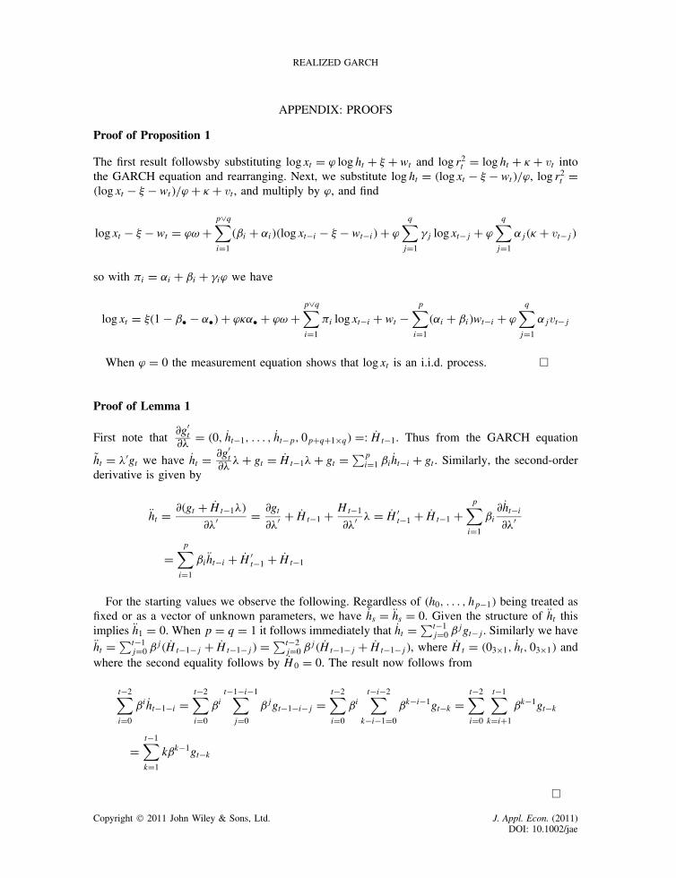
REALIZED GARCH
APPENDIX: PROOFS
Proof of Proposition 1
The first result followsby substituting log xt D ϕ log ht C � C wt and log r2t D log ht C � C vt into
the GARCH equation and rearranging. Next, we substitute log ht D �log xt � � � wt�/ϕ, log r2t D
�log xt � � � wt�/ϕ C � C vt, and multiply by ϕ, and find
log xt � � � wt D ϕω Cp_q∑iD1
�ˇi C ˛i��log xt�i � � � wt�i�C ϕq∑jD1
�j log xt�j C ϕq∑jD1
˛j�� C vt�j�
so with i D ˛i C ˇi C �iϕ we have
log xt D ��1 � ˇž � ˛ž�C ϕ�˛ž C ϕω Cp_q∑iD1
i log xt�i C wt �p∑iD1
�˛i C ˇi�wt�i C ϕq∑jD1
˛jvt�j
When ϕ D 0 the measurement equation shows that log xt is an i.i.d. process. �
Proof of Lemma 1
First note that∂g0t
∂� D �0, Pht�1, . . . , Pht�p, 0pCqC1ðq� D: PHt�1. Thus from the GARCH equation
Qht D �0gt we have Pht D ∂g0t
∂� �C gt D PHt�1�C gt D ∑piD1 ˇi Pht�i C gt. Similarly, the second-order
derivative is given by
Rht D ∂�gt C PHt�1��
∂�0 D ∂gt∂�0 C PHt�1 C Ht�1
∂�0 � D PH0t�1 C PHt�1 C
p∑iD1
ˇi∂ Pht�i∂�0
Dp∑iD1
ˇi Rht�i C PH0t�1 C PHt�1
For the starting values we observe the following. Regardless of �h0, . . . , hp�1� being treated asfixed or as a vector of unknown parameters, we have Phs D Rhs D 0. Given the structure of Rht thisimplies Rh1 D 0. When p D q D 1 it follows immediately that Pht D ∑t�1
jD0 ˇjgt�j. Similarly we have
Rht D ∑t�1jD0 ˇ
j� PHt�1�j C PHt�1�j� D ∑t�2jD0 ˇ
j� PHt�1�j C PHt�1�j�, where PHt D �03ð1, Pht, 03ð1� andwhere the second equality follows by PH0 D 0. The result now follows from
t�2∑iD0
ˇi Pht�1�i Dt�2∑iD0
ˇit�1�i�1∑jD0
ˇjgt�1�i�j Dt�2∑iD0
ˇit�i�2∑
k�i�1D0
ˇk�i�1gt�k Dt�2∑iD0
t�1∑kDiC1
ˇk�1gt�k
Dt�1∑kD1
kˇk�1gt�k
�
Copyright 2011 John Wiley & Sons, Ltd. J. Appl. Econ. (2011)DOI: 10.1002/jae

P. R. HANSEN, Z. HUANG AND H. H. SHEK
Proof of Proposition 2
Recall that ut D Qxt � 0mt and Qht D g0t�. Thus the derivatives with respect to Qht are given by
∂zt
∂ QhtD∂rt exp
(�1
2Qht)
∂ QhtD �1
2zt so that
∂z2t
∂ QhtD �z2
t ,
Put D ∂ut
∂ QhtD �ϕ C 1
2zt�
0 Pat, and Rut D ∂ Put∂ Qht
D∂
(�ϕ C 1
2zt Pa�zt�0�
)∂ Qht
D �1
4� 0�zt Pat C z2
t Rat�
Thus with �t D �12 fQht C z2
t C log��2u �C u2
t /�2ug we have
∂�t∂ut
D 2ut�2u
and∂�t
∂ QhtD �1
2
{1 C ∂z2
t
∂ QhtC ∂u2
t /∂ Qht�2u
}D �1
2
{1 � z2
t C 2ut Put�2u
}
Derivatives with respect to � are ∂zt∂� D ∂zt
∂ Qht∂ Qht∂� D �1
2 ztPht, ∂ut∂� D ∂ut
∂ Qht∂ Qht∂� D Put Pht, ∂ Put
∂�0 D Rut Ph0t,
and ∂�t∂� D ∂�t∂ Qht
Pht D �12
{1 � z2
t C 2ut Put�2u
}Pht. Derivatives with respect to are ∂ut∂� D �1, ∂ Put
∂� D0, ∂�t∂� D ∂�t
∂ut∂ut∂� D �2 ut
�2u
, ∂ut∂ϕ D �Qht, ∂ Put∂ϕ D �1, ∂�t∂ϕ D ∂�t
∂ut∂ut∂ϕ D �2 ut
�2u
Qht, ∂ut∂� D �at, ∂ Put∂� D
12 zt Pat,
∂�t∂� D ∂�t
∂ut∂ut∂� D �2 ut
�2u
at. Similarly, ∂�t∂�2u
D �12 ��
�2u � u2
t ��4u �. Now we turn to the second-
order derivatives:
�2∂2�t∂�∂�0 D Pht
{�∂z
2t
∂�0 C 2
�2u
(Put ∂ut∂�0 C ut
∂ Put∂�0
)}C(
1 � z2t C 2ut
�2u
Put)∂ Pht∂�0
D Pht{z2t C 2
�2u
� Pu2t C ut Rut�Ph0
t
}C(
1 � z2t C 2ut
�2u
Put)
Rht
Similarly, since ∂zt∂ D 0 we have
�2∂2�t∂�∂�
D∂
(1 � z2
t C 2ut�2u
Put)
Pht∂�
D 2Pht(∂ut∂ 0
Put�2u
C ut�2u
∂ Put∂�
)D 2Pht
(� Put�2u
C 0
)
�2∂2�t∂�∂ϕ
D∂
(1 � z2
t C 2ut�2u
Put)
Pht∂ϕ
D 2Pht(∂ut∂ϕ
Put�2u
C ut�2u
∂ Put∂ϕ
)D 2Pht
(�Qht Put
�2u
� ut�2u
)
�2∂2�t∂�∂� 0 D 2Pht
(∂ut∂� 0
Put�2u
C ut�2u
∂ Put∂� 0
)D 2Pht
(�a0
t
Put�2u
C ut�2u
1
2zt Pat
)
Copyright 2011 John Wiley & Sons, Ltd. J. Appl. Econ. (2011)DOI: 10.1002/jae

REALIZED GARCH
so that
∂2�t∂�∂ 0 D Put
�2u
Phtm0t C ut
�2u
Phtb0t, with bt D
(0, 1,�1
2zt Pa0
t
)0,
∂2�t∂�∂�2
u
D �1
2
∂
(1 � z2
t C 2ut�2u
Put)
Pht
∂�2u
D ut Put Pht�4u
,∂2�t∂ ∂ 0 D � 1
�2u
mtm0t,
∂2�t∂ ∂�2
u
DD �1
2
(�2ut�4u
)mt D ut
�4u
mt,∂2�t∂�2u∂�
2u
D �1
2
(�1
�4u
C 2u2t
�6u
)D 1
2
�2u � 2u2
t
�6u
�
Lemma 2. Let W D �1ZC �2�Z2 � 1�CU, where Z ∼ N�0, 1� and U ∼ N�0, �2u �. Then
E�expfi�Wg� D 1√1 � 2i��2
exp
{2i�2�2
1
2�1 � 2i��2�� i��2 C 2i�2�2
u
2
}
Proof. We have E�eaZC b2 �Z2�1�� equals
∫ 1
�1eazC
b2 �z
2�1� 1p2ez2
2 dz D∫ 1
�1
1p2e
a2
2�1�b�� b2 � 12
�z� a1�b �
�1�b��1 �dz D 1p1 � b
ea2
2�1�b�� b2
and from the moment-generating function for the Gaussian distribution we have E�ecU� Dec2�2
u2 . Since Z and U are independent, we have E�expfi�Wg� D E�expfi��1ZC i��2�Z2 �
1�g�E�expfi�Ug� D 1√1 � 2i��2
e2i�2�2
12�1�2i��2�
�i��2e2i�2�2
u2 .
�
Proof of Proposition 4
We note that
ht D exp
( 1∑iD0
i�C �wt�1�
)D e
1�
1∏iD0
E exp��i��zt�i��E�expfi�ut�ig�,
h2t D exp
(2
1∑iD0
i�C �wt�1�
)D e
21�
1∏iD0
E exp�2�i��zt�i��E�expf2i�ut�ig�
and using results such as Lemma 2 and
E
( 1∏iD0
expfi�ut�ig)
D1∏iD0
E�expfi�ut�ig� D1∏iD0
e2i�2�2
u2 D e
∑1iD0
2i�2�2u
2 D e�2�2
u /21�2
Copyright 2011 John Wiley & Sons, Ltd. J. Appl. Econ. (2011)DOI: 10.1002/jae
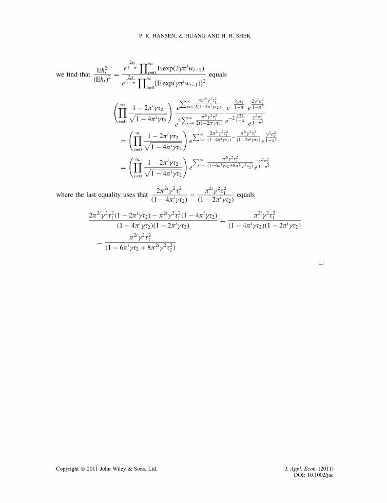
P. R. HANSEN, Z. HUANG AND H. H. SHEK
we find thatEh2
t
�Eht�2 D
e2
1�∏1
iD0E exp�2�iwt�1�
e2
1�∏1
iD0fE exp��iwt�1�g2
equals
( 1∏iD0
1 � 2i��2√1 � 4i��2
)e∑1
iD0
42i�2�21
2�1�4i��2�
e2∑1
iD0
2i�2�21
2�1�2i��2�
e� 2��21�
e�2��2
1�
e2�2�2
u1�2
e�2�2
u1�2
D( 1∏iD0
1 � 2i��2√1 � 4i��2
)e∑1
iD0
22i�2�21
�1�4i��2�� 2i�2�2
1�1�2i��2� e
�2�2u
1�2
D( 1∏iD0
1 � 2i��2√1 � 4i��2
)e
∑1iD0
2i�2�21
�1�6i��2C82i�2�22 � e
�2�2u
1�2
where the last equality uses that22i�2�2
1
�1 � 4i��2�� 2i�2�2
1
�1 � 2i��2�equals
22i�2�21�1 � 2i��2�� 2i�2�2
1 �1 � 4i��2�
�1 � 4i��2��1 � 2i��2�D 2i�2�2
1
�1 � 4i��2��1 � 2i��2�
D 2i�2�21
�1 � 6i��2 C 82i�2�22�
�
Copyright 2011 John Wiley & Sons, Ltd. J. Appl. Econ. (2011)DOI: 10.1002/jae