REALIZATION SPACES OF POLYTOPES - CiteSeer
198
REALIZATION SPACES OF POLYTOPES by J¨ urgen Richter-Gebert Technische Universit¨ at Berlin, 1996
Transcript of REALIZATION SPACES OF POLYTOPES - CiteSeer
REALIZATION SPACES
OF POLYTOPES
by
Jurgen Richter-Gebert
Technische Universitat Berlin, 1996

Manuscript, July 1996
Techniche Universitat Berlin
Author’s address: Dr. Dr. Jurgen Richter-Gebert
Technische Universitat Berlin,
FB Mathematik, Sekr. 6-1,
Straße des 17. Juni 136,
D-10623 Berlin, Germany
e-mail: [email protected]
Keywords:
Polytopes, realization spaces, Steinitz’s Theorem, universality, oriented ma-troids, semialgebraic sets, stable equivalence, NP-completeness
1991 Mathematics Subject Classification:
Primary: 52B11, 52B40;
Secondary: 14P10, 51A25, 52B10, 52B30, 68Q15.
Supported by a DFG Gerhard-Hess-Forschungsforderungspreis Zi 475/1-1:,,Methoden der kombinatorischen Geometrie“ awarded to Prof. Dr. G.M. Ziegler

v
For Ingrid and Angela-Sophia,
who helped me so much.

vi

Preface
Steinitz’s Theorem (proved in 1922) is one of the oldest and most prominentresults in polytope theory. It gives a completely combinatorial characterization ofthe face lattices of 3-dimensional polytopes. Steinitz observed that the techniqueof proving his theorem also implies that for any 3-dimensional polytope theset of all its realizations is a trivial topological set. In other words: realizationspaces of 3-dimensional polytopes are contractible. For a long time it was anopen problem whether there exist similar results in spaces of dimension greaterthan three. It was proved by Mnev in 1986 that the contrary is the case. As aconsequence of his famous Universality Theorem for oriented matroids he showedthat realization spaces of polytopes with dimension-plus-four vertices can havearbitrary homotopy type. The present research monograph studies the structureof realization spaces of polytopes in fixed dimension. The main result that isobtained is a Universality Theorem for 4-polytopes. It states that for everyprimary basic semialgebraic set V there exists a 4-dimensional polytope whoserealization space is stably equivalent to V .
This research monograph has three goals. First of all it serves as a compre-hensive source for all results that I have been able to obtain in connection to theUniversality Theorem for 4-polytopes. It includes complete proofs of all theseresults including a proof of the Universality Theorem itself. Secondly, it is (as thetitle says) meant as an introduction to the beautiful theory of realization spacesof polytopes. For that purpose also a treatment of Steinitz’s Theorem is included.Although the result is classical the proof presented here contains some new andfresh elements. In particular, we provide a new proof for Tutte’s Theorem onequilibrium representations of planar graphs. We also give a complete proof ofMnev’s Universality Theorem for oriented matroids (and of its generalization:the Universal Partition Theorem). Last but not least, this monograph is writ-ten for the sake of enjoyment of geometric constructions. Most of the conceptsand constructions that are needed here are elementary in nature. The final con-struction for the Universality Theorem is obtained by building larger and largerpolytopal units of increasing geometric and algebraic complexity. We start fromsmall incidence configurations, go to polytopes for addition and multiplication,and end up with polytopes that encode entire polynomial inequality systems. Ihope that the reader can feel the fun that lies in these constructions.
There are many alternative ways of approaching the main results of thismonograph. In particular, there are several different ways to build up the proof
vii

viii preface
of the Universality Theorem for 4-polytopes. However, all the approaches kownto me rely on similar principles:
• first construct small and useful polytopes (using Lawrence Extensions orsimilar techniques) that have non-prescribable facets (or vertex figures),
• use connected sums to join these polytopes to larger units that are capableof encoding arithmetic operations,
• finally use connected sums to join these arithmetic units into even largerpolytopes that encode entire polynomial inequality systems.
Here I have chosen an approach that is very modular. The basic building blocksare very simple polytopes, and the whole complexity is governed by the way ofcomposing these blocks.
In order to obtain the strongest possible results it was necessary to setup a new concept of stable equivalence that compares realization spaces withother semialgebraic sets. The reader may excuse the fact that whenever stableequivalence between two spaces is proved the exposition becomes a bit techni-cal. Everywhere else I used concrete geometric approaches rather than abstractsettings. Whenever it is possible the constructions are carried out in an explicitmanner.
Part I to Part III are based on my Habilitationsschrift at the TechnicalUniversity Berlin, 1995. The typesetting of this monograph relies on LATEX.Most of the drawings are done with Cinderella.
There are many people who have made the writing of this monograph pos-sible. First of all I want to thank Gunter M. Ziegler for offering me a positionwhere I could concentrate mainly on this work. I am extremely grateful to himfor his careful reading of every page and for the uncountably many valuable sug-gestions, discussions, comments and protests that encouraged me to go alwaysone step further than I had already done.
Also I am very grateful to Anders Bjorner, Marie-Francoise Coste-Roy,Henry Crapo, Eva-Maria Feichtner, Eli Goodman, Martin Henk, Peter Klein-schmidt, Ulli H. Kortenkamp, Peter McMullen, Ricky Pollack, Jorg Rambau,and Bernd Sturmfels for many inspiring discussions and valuable comments onmy manuscript in its various stages.
I especially, want to thank my wife Ingrid and my little daughter Angela-Sophia, who was born on the day of the “breakthrough” for the main theorem.Angela-Sophia’s inspiring presence definitely helped me to keep my thoughts assimple as possible. Without Ingrid I would have never been able to write allthis. She always had an open ear for me that helped me to clarify my ideas, andshe accompanied me through all the “dead ends” that are unavoidable in sucha kind of work.
Berlin, October 1996 Jurgen Richter-Gebert

Contents
Preface vii
Introduction 1
1 Polytopes and their Realizations . . . . . . . . . . . . . . . . . . 1
1.1 Polytopes . . . . . . . . . . . . . . . . . . . . . . . . . . . 1
1.2 History I: Steinitz’s Theorem . . . . . . . . . . . . . . . . 3
1.3 History II: Polytopes in Dimension Higher than 3 . . . . . 4
1.4 New Results on 4-Polytopes . . . . . . . . . . . . . . . . . 6
1.5 Polytopal Tools . . . . . . . . . . . . . . . . . . . . . . . . 7
1.6 Sketch of the Proof of the Universality Theorem . . . . . 8
1.7 Outline of the Monograph . . . . . . . . . . . . . . . . . . 10
Part I: The Objects and the Tools 13
2 Polytopes and Realization Spaces . . . . . . . . . . . . . . . . . . 13
2.1 Notational Conventions . . . . . . . . . . . . . . . . . . . 13
2.2 Polytopes, Cones and Combinatorial Polytopes . . . . . . 15
2.3 Affine and Projective Equivalence . . . . . . . . . . . . . 18
2.4 Realization Spaces . . . . . . . . . . . . . . . . . . . . . . 19
2.5 Semialgebraic Sets and Stable Equivalence . . . . . . . . . 20
2.6 Polarity . . . . . . . . . . . . . . . . . . . . . . . . . . . . 24
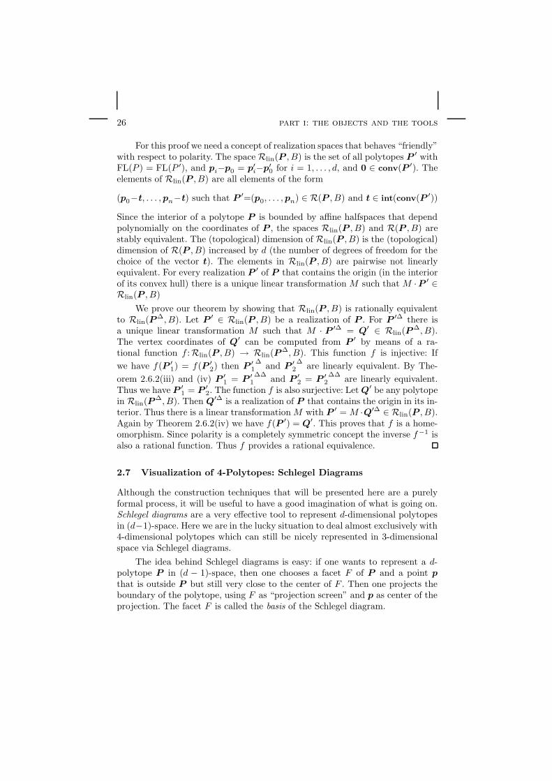
2.7 Visualization of 4-Polytopes: Schlegel Diagrams . . . . . . 26
3 Polytopal Constructions . . . . . . . . . . . . . . . . . . . . . . . 28
3.1 Pyramids, Prisms and Tents . . . . . . . . . . . . . . . . . 28
3.2 Connected Sums . . . . . . . . . . . . . . . . . . . . . . . 29
3.3 Lawrence Extensions . . . . . . . . . . . . . . . . . . . . . 32
3.4 Examples . . . . . . . . . . . . . . . . . . . . . . . . . . . 37
Part II: The Universality Theorem 41
4 Equations and Polytopes . . . . . . . . . . . . . . . . . . . . . . . 41
4.1 Shor’s Normal Form . . . . . . . . . . . . . . . . . . . . . 41
ix

x contents
4.2 Encoding Equations into Polygons . . . . . . . . . . . . . 42
5 The Basic Building Blocks . . . . . . . . . . . . . . . . . . . . . . 45
5.1 A Transmitter . . . . . . . . . . . . . . . . . . . . . . . . 46
5.2 The Connector . . . . . . . . . . . . . . . . . . . . . . . . 47
5.3 A Forgetful Transmitter . . . . . . . . . . . . . . . . . . . 48
5.4 A 4-Polytope with Non-Prescribable 2-Face . . . . . . . . 50
5.5 An Adapter . . . . . . . . . . . . . . . . . . . . . . . . . . 51
5.6 A Polytope for Partial Transmission of Information . . . . 52
5.7 A Transmitter for Line Slopes . . . . . . . . . . . . . . . . 53
6 Harmonic Sets and Octagons . . . . . . . . . . . . . . . . . . . . 55
6.1 A Line Configuration Forcing Harmonic Relations . . . . 55
6.2 The Harmonic Polytope . . . . . . . . . . . . . . . . . . . 56
7 Polytopes for Addition and Multiplication . . . . . . . . . . . . . 59
7.1 Addition . . . . . . . . . . . . . . . . . . . . . . . . . . . . 59
7.2 Multiplication . . . . . . . . . . . . . . . . . . . . . . . . . 62
8 Putting the Pieces Together: The Universality Theorem . . . . . 68
8.1 Encoding Semialgebraic Sets in Polytopes . . . . . . . . . 68
8.2 The Construction Seen from a Distance . . . . . . . . . . 69
8.3 Proving Stable Equivalence . . . . . . . . . . . . . . . . . 71
Part III: Applications of Universality 77
9 Complexity Results . . . . . . . . . . . . . . . . . . . . . . . . . . 77
9.1 Algorithmic Complexity . . . . . . . . . . . . . . . . . . . 77
9.2 Algebraic Complexity . . . . . . . . . . . . . . . . . . . . 78
9.3 The Sizes of 4-Polytopes . . . . . . . . . . . . . . . . . . . 81
9.4 Infinite Classes of Non-Polytopal Combinatorial 3-Spheres 83
10 Universality for 3-Diagrams and 4-Fans . . . . . . . . . . . . . . 87
10.1 3-Diagrams and 4-Fans . . . . . . . . . . . . . . . . . . . 87
10.2 The Polytope PP ′(S) . . . . . . . . . . . . . . . . . . . . . 90
10.3 Nets . . . . . . . . . . . . . . . . . . . . . . . . . . . . . . 92
10.4 The Corollaries . . . . . . . . . . . . . . . . . . . . . . . . 95
11 The Universal Partition Theorem for 4-Polytopes . . . . . . . . . 97
11.1 Semialgebraic Families and Partitions . . . . . . . . . . . 97
11.2 Shor’s Normal Form Versus Quadrilateral Sets . . . . . . 99
11.3 Computations of Polynomials . . . . . . . . . . . . . . . . 101
11.4 Encoding Quadrilateral Sets into Polytopes . . . . . . . . 106
11.5 The “Switch Polytope” . . . . . . . . . . . . . . . . . . . 107
11.6 The Universal Partition Theorem . . . . . . . . . . . . . . 110
11.7 The Universal Partition Theorem for Point Configurations 112
contents xi
Part IV: Three-dimensional Polytopes 117
12 Graphs . . . . . . . . . . . . . . . . . . . . . . . . . . . . . . . . . 118
12.1 Preliminaries from Graph Theory . . . . . . . . . . . . . . 118
12.2 Tutte’s Theorem on Stresses in Graphs . . . . . . . . . . 122
13 3-Polytopes . . . . . . . . . . . . . . . . . . . . . . . . . . . . . . 133
13.1 From Stressed Graphs to Polytopes . . . . . . . . . . . . . 133
13.2 A Quantitative Analysis . . . . . . . . . . . . . . . . . . . 140
13.3 The Structure of the Realization Space . . . . . . . . . . . 144
Part V: Alternative Construction Techniques 149
14 Generalized Adapter Techniques . . . . . . . . . . . . . . . . . . 149
15 A Non-Steinitz Theorem in Dimension Five . . . . . . . . . . . . 151
15.1 Conics and Incidence Theorems . . . . . . . . . . . . . . . 151
15.2 An Incidence Theorem for 4-Polytopes . . . . . . . . . . . 156
15.3 The Non-Steinitz Theorem . . . . . . . . . . . . . . . . . 160
16 The Universality Theorem in Dimension 6 . . . . . . . . . . . . . 162
16.1 Oriented Matroids . . . . . . . . . . . . . . . . . . . . . . 163
16.2 Zonotopes and Planets . . . . . . . . . . . . . . . . . . . . 165
16.3 The Construction . . . . . . . . . . . . . . . . . . . . . . . 169
Part VI: Problems 173
17 Open Problems on Polytopes and Realization Spaces . . . . . . . 173
17.1 Universality Theorems for Simplicial Polytopes . . . . . . 173
17.2 Small Non-Rational 4-Polytopes . . . . . . . . . . . . . . 174
17.3 Many Polytopes . . . . . . . . . . . . . . . . . . . . . . . 174
17.4 The Sizes of Polytopes . . . . . . . . . . . . . . . . . . . . 175
17.5 Rational Realizations of 3-Polytopes . . . . . . . . . . . . 176
17.6 The Steinitz Problem for Triangulated Tori . . . . . . . . 176

Introduction
1 Polytopes and their Realizations
Polytopes have a long tradition as objects of mathematical study. Their historicalroots reach back to the ancient Greek mathematicians, having a first highlightin their enumeration of the famous Platonic Solids. Already at this point strongimpetus came from the fact that polytopes intimately connect topics from ge-ometry and from combinatorics (the Platonic Solids solve a first enumerativequestion in polytopal geometry, to find all polytopes with a flag transitive sym-metry group — a combinatorial concept). The work presented in this researchmonograph is also motivated from questions that are on the borderline of geom-etry, algebra and combinatorics. We investigate the structure of the realizationspaces of polytopes with fixed combinatorial types. Our aim is to exhibit a radicalcontrast between the behavior of realization spaces for polytopes in dimensionsthree and four.
For three-dimensional polytopes the structure of the realization spaces turnsout to be rather simple (a consequence of the classical Steinitz’s Theorem thatwas already known in 1922). However, realization spaces of four-dimensionalpolytopes can behave as complicated as one can think of (as a consequence of theUniversality Theorem first presented in this monograph). We will give completeproofs of these two theorems and explore their far reaching consequences.
1.1 Polytopes
Formally, polytopes are the convex hulls of finite point sets in Rd:
Definition 1. Let P = (p1, . . . ,pn) ∈ Rd·n be a finite collection of points that
affinely span Rd. The set
P = conv(P ) := n∑
i=1
λipi |n∑
i=1
λi = 1 and λi ≥ 0 for i = 1, . . . , n,
the convex hull of the point set P , is called a d-dimensional polytope (a “d-polytope” for short). The faces of P are P itself and the intersections P ∩A, suchthat A is an affine hyperplane that does not meet the interior of P. The facelattice of P is the set of all faces of P , partially ordered by inclusion.
1

2 introduction
(a) (b)
Figure 1: A convex polygon and a cube. Two simple examples of polytopes.
While a polytope is a geometric object, its face lattice is purely combi-natorial in nature. Figure 1(a) illustrates a 2-polytope as the convex hull of afinite number of points in the plane. We see that those points that are not inan extreme position make no contribution to the polytope itself. The points inextreme position (i.e., the 0-dimensional faces) are the vertices of a polytope.Figure 1(b) shows a cube as an example of a 3-dimensional polytope. The facelattice of the cube consists of the cube itself, 6 facets, 12 edges, 8 vertices andthe empty set.
The need to structure the set of all polytopes of a fixed dimension leads totwo main lines of study:
• to list all possible combinatorial types of polytopes (in other words, todetermine which finite lattices correspond to face lattices of polytopes, andwhich do not),
• to describe the set of all realizations of a given combinatorial type.
The “set of all realizations” of a combinatorial type is formalized below bythe concept of the realization space of a polytope. Besides their intrinsic impor-tance for questions of real discrete geometry, such spaces appear in subjects asdiverse as algebraic geometry (moduli spaces), differential topology (see Cairns’smoothing theory [21]), and nonlinear optimization (see Gunzel et al. [33]).
Assume that in Definition 1 each point pi for i = 1, . . . , n is a vertex of P .A realization of a polytope P is a polytope Q = conv(q1, . . . , qn) such that theface lattices of P and Q are isomorphic under the correspondence pi → qi. Thesequence of vertices B = (p1, . . . ,pd+1) is a basis of P if these points are affinelyindependent in any realization of P .

polytopes and their realizations 3
Definition 2. Let P = conv(p1, . . . ,pn) ⊂ Rd be a d-polytope with n vertices
and with a basis B = (p1, . . . ,pd+1). The realization space R(P,B) is the set
of all matrices Q = (q1, . . . , qn) ∈ Rd·n for which conv(Q) is a realization of Pand qi = pi for i = 1, . . . , d+ 1.
By the choice of a certain basis for which the points have to stay fixed,we factor out components in the set of all realizations of a polytope that comefrom rotations and translations. It turns out that the realization space R(P,B)is essentially (up to “stable equivalence,” see below) independent of the choiceof an admissible basis. Hence it makes sense to speak of the realization spaceR(P ) of a polytope.
Every realization space is a primary basic semialgebraic set: it is the set ofsolutions of a finite system of polynomial equations fi(x) = 0 and strict inequal-ities gj(x) > 0, where the fi and gj are polynomials with integer coefficients
on Rd·n. To see this, one checks that the realization space is the set of all matri-ces Q ∈ R
d·n for which some entries are fixed, and the determinants of certaind× d minors have to be positive, negative, or zero.
Our main aim here is a Universality Theorem for 4-polytopes, stating thatfor every primary semialgebraic V set there exists a 4-polytope whose realizationspace is “stably equivalent” to V . The concept of stable equivalence will beclarified in Section 2. It can be considered as a strengthened version of homotopyequivalence that preserves also information on the underlying algebraic structure.In particular, if two semialgebraic sets V and V ′ are stably equivalent and Vcontains non-rational points, then V ′ contains non-rational points as well.
1.2 History I: Steinitz’s Theorem
What does the realization space of a polytope look like? Which algebraic numbersare needed to coordinatize the vertex set of a given d-dimensional polytope? Howcan one tell whether a finite lattice is the face lattice of a polytope or not?
For 3-dimensional polytopes, Steinitz’s work [56, 55] answered the basicquestions about realization spaces more then seventy years ago. In particular,Steinitz’s “Fundamentalsatz der konvexen Typen” (today known as Steinitz’sTheorem) and its modern relatives (see [31] and [65]) provide complete answersto the above questions for this special case.
Steinitz’s Theorem (1922): A graph G is the edge graph of a 3-polytope ifand only if G is simple, planar and 3-connected.
The classical proof by Steinitz is done by a clever combinatorial reductiontechnique that allows one to generate larger 3-polytopes from smaller ones. Al-ternatively, Steinitz’s Theorem can be proved using the Koebe-Andreev-ThurstonCircle Packing Theorem (see [65]), or by arguments using the concept of self-stresses of planar graphs (see [23, 36, 47], and Part IV). The statements in the

4 introduction
following list can be derived from a careful inspection of the known proofs ofSteinitz’s Theorem.
• For every 3-polytope P ⊆ R3 the realization space R(P ) is a smooth openball. (This ball has dimension e− 6, if P has e edges.)
• For every 3-polytope P the space R(P ) contains rational points, that is,every 3-polytope can be realized with integral vertex coordinates.
• Every combinatorial 2-sphere is polytopal.
• Barnette, Grunbaum, 1970, [12]: The shape of one 2-face in the bound-ary of a 3-polytope P can be arbitrarily prescribed, that is, the canonicalmap R(P )→ R(F ) is surjective for every facet F ⊆ P .
• Onn, Sturmfels, 1992, [51]: If a 3-polytope has n vertices then it can be
realized with integral coefficients smaller than n169n3
.
In Part IV of this monograph we will present a proof of Steinitz’s Theorem that isbased on the self stress approach. This approach also proves that the realizationspace of any 3-polytope is contractible, and that it contains rational points. Inparticular, our treatment will improve the bound given by Sturmfels and Onn.
• Any 3-polytope P with n vertices can be realized with integral coordinatessmaller than 218n2
.
• If P furthermore contains a triangle, then it can be realized with integralcoordinates smaller than 43n.
One can prove statements similar to the above corollaries for d-polytopesthat have at most d+3 vertices. Under (affine) Gale duality these polytopes areencoded by certain point arrangements on a line. This fact leads to a classificationmethod that allows one to analyze these polytopes. Most of this analysis has beendone by Mani [44] and Kleinschmidt [41].
• Every combinatorial (d−1)-sphere with d+ 3 vertices is polytopal.
• Every d-polytope with d+3 vertices can be realized with integral coefficients.
• The realization space of every d-polytope with d+3 vertices is contractible.
1.3 History II: Polytopes in Dimension Higher than 3
Over the years, it became clear that no similar positive answer could be expectedfor high-dimensional polytopes. The situation becomes much more complicatedif either the dimension or the codimension exceeds three. We first discuss thecase of fixed dimension. There are several d-polytopes (with d ≥ 3) known thatbehave differently from 3-polytopes with respect to realizability. The followinglist summarizes chronologically the counterexamples that are found to contrastwith the 3-dimensional case.
• Perles, 1967, [31]:Non-rational 8-polytope (12 vertices, 28 facets).

polytopes and their realizations 5
• Barnette, 1971, [8]:Non-polytopal combinatorial 3-sphere (8 vertices, 19 facets).
• Kleinschmidt, 1976, [40]:4-polytope with non-prescribable 3-face (10 vertices, 15 facets).
• Barnette, 1980, [11]:4-polytope with non-prescribable 3-face (12 vertices, 7 facets).
• Bokowski, Ewald, Kleinschmidt, 1984, [15, 16]:4-polytope with disconnected realization space (10 vertices, 28 facets).
• Ziegler, 1992, [65]:5-polytope with non-prescribable 2-face (12 vertices, 10 facets).
Besides these “sporadic examples,” no general construction technique wasknown to produce polytopes with a “controllably bad” behavior for any fixeddimension. The σ-construction presented in [57] for that purpose turned out tobe incorrect [65].
If we investigate the case of codimension four much more is known andgeneral tools are applicable. In 1986 N.E. Mnev proved a Universality Theoremfor oriented matroids of rank 3 (see [7, 33, 52, 48, 49]). This result leads, viaGale diagram techniques, to a universality theorem for d-polytopes with d + 4vertices: in general for such polytopes the realization spaces can be arbitrarilycomplicated. In technical terms the Universality Theorem can be stated as:
Mnev’s Universality Theorem (1986):
(i) For every primary basic semi-algebraic set V defined over Z there is a rank3 oriented matroid whose realization space is stably equivalent to V .
(ii) For every primary basic semi-algebraic set V defined over Z there is aninteger d > 1 and a d-polytope P with d+4 vertices whose realization spaceis stably equivalent to V .
Stable equivalence is a strong concept of topological equivalence, that inparticular preserves homotopy type and the algebraic complexity of test points.So Mnev’s construction implies:
• The realizability problem for d-polytopes with d+ 4 vertices is (polynomialtime) equivalent to the “Existential Theory of the Reals.”
• The realizability problem for d-polytopes with d+ 4 vertices is NP-hard.
• All algebraic numbers are needed to coordinatize all d-polytopes with d+ 4vertices.
• For every finite simplicial complex ∆ there is a d-polytope with d+4 verticeswhose realization space is homotopy equivalent to ∆.
It will be the main purpose of this monograph to establish similar results for thecase of polytopes in fixed dimension d = 4.

6 introduction
1.4 New Results on 4-Polytopes
We will constructively prove that the realization spaces of 4-polytopes can be“arbitrarily ugly,” in a well defined sense.
Universality Theorem for 4-Polytopes:For every primary basic semi-algebraic set V defined over Z, there is a 4-polytopeP whose realization space is stably equivalent to V . The face lattice of P can begenerated from defining equations of V in polynomial time.
The following new results are corollaries of the Universality Theorem or conse-quences of the construction we provide for it.
(i) There is a non-rational 4-polytope with 33 vertices.
(ii) All algebraic numbers are needed to coordinatize all 4-polytopes.
(iii) The realizability problem for 4-polytopes is NP-hard.
(iv) The realizability problem for 4-polytopes is (polynomial time) equiva-lent to the “Existential Theory of the Reals” (see [53]).
(v) For every finite simplicial complex ∆, there is a 4-polytope whose re-alization space is homotopy equivalent to ∆.
(vi) There is a 4-polytope for which the shape of some 2-face cannot bearbitrarily prescribed.
(vii) Polytopality of 3-spheres cannot be characterized by excluding a finiteset of “forbidden minors”.
(viii) In order to realize all combinatorial types of integral 4-polytopes withn vertices in the integer grid 1, 2, . . . , f(n)4, the “coordinate size”function f(n) has to be at least doubly exponential in n.
In particular these consequences solve all the problems that were recentlyemphasized in Ziegler’s article “Three problems about 4-polytopes” [64].
The proof of the Universality Theorem is constructive. We will describe 4-polytopes that model addition and multiplication by the non-prescribability ofa 2-dimensional face. The addition- and multiplication-polytopes will be joinedinto larger units that model systems of polynomial equations and inequalities.
Our approach is in some sense analogous to Mnev’s original proof of hisUniversality Theorem for oriented matroids. He uses the classical von Staudtconstructions (which model addition and multiplication for points on a line inthe projective plane) to compose large planar incidence structures that modelarbitrary polynomial computations. The main difficulty in Mnev’s proof is toorganize the construction in a way such that different basic calculations do notinterfere and such that the underlying oriented matroid stays invariant for all in-stances of a geometric computation. Our main difficulty will be the constructionof polytopes for addition and multiplication.

polytopes and their realizations 7
1.5 Polytopal Tools
Lawrence extensions and connected sums are elementary geometric operationson polytopes that form the basis for the constructions we need in order to provethe Universality Theorem. They are very simple and innocent looking operations,but they are very powerful.
For Lawrence extensions the basic operation is the following: take a pointp in a d-dimensional point configuration, and replace it by two new pointsp and p that lie on a ray that starts at the original point and leaves the d-dimensional space spanned by the point configuration in a “new” direction of(d+ 1)-dimensional space (see Figure 2).
p
p
p
R2
R3
Figure 2: A Lawrence extension of a pentagon.
Every such Lawrence extension increases both the dimension of a pointconfiguration and its number of points by 1. Note that although the originalpoint is deleted in the construction, it is still implicitly present: it can be “re-constructed” as the intersection of the line spanned by the two new points withthe d-hyperplane spanned by the original point configuration.
The “classical” use of Lawrence extensions [13, 6, 49] starts with a 2-dimensional configuration of n points, and performs Lawrence extensions on allthese points, one by one. The resulting configuration of 2n points is the vertexset of an (n+2)-dimensional polytope, the Lawrence polytope of the point config-uration. Every realization of the Lawrence polytope determines a realization ofthe original point configuration, including all collinearities and all orientationsof triples. In fact, the realization spaces of the Lawrence polytope and the planarconfiguration are stably equivalent. This can be used to lift Mnev’s UniversalityTheorem from planar point configurations (oriented matroids) to d-polytopes.
If one wants to stay within the realm of 4-polytopes, then it is not permissi-ble to use more than two Lawrence extensions. However, careful use of just one

8 introduction
or two Lawrence extensions on some points outside a 2- or 3-polytope leads toextremely interesting and useful polytopes — such as the basic building blocksfor the Universality Theorem (see Section 5).
Connected sums are the operations that compose these basic building blocksinto larger units. They are performed as follows: Assume that one is given twod-polytopes P1 and P2 that have projectively equivalent facets F1 resp. F2. Weuse F to denote the combinatorial type of F1
∼= F2. Then, using a projectivetransformation, one can “merge” P1 and P2 into a more complicated polytope,the connected sum Q := P1#F
P2. The polytope Q has all the facets of P1 andP2, except for F1 and F2. However, the boundary complex ∂F , consisting of allthe proper faces of F , is still present in Q (Figure 3).
−→
P1 P2
F1 F2
P1#FP2
Figure 3: The connected sum of a cube and a triangular prism.
Now, if one takes an arbitrary realization of Q, then it is not in general truethat this realization arises as a connected sum of realizations of P1 and of P2:in a “bad” realization of Q the boundary complex ∂F may not be flat. In fact,in dimension d = 3 one can see that the complex ∂F in Q is necessarily flat ifand only if F is a triangular facet. In dimension 4, there are much more differenttypes of facets that are “necessarily flat,” among them pyramids, prisms, and“tents.” Only such necessarily flat facets are used in connected sum operationsfor the proof of the Universality Theorem.
1.6 Sketch of the Proof of the Universality Theorem
Our proof starts from the defining equations of a primary basic semialgebraicset, and uses them explicitly to construct the face lattice of a 4-polytope. Aresult of Shor [53] is used, which states that every primary semialgebraic set Vis stably equivalent to a semialgebraic set V ′ ∈ R
n whose variables
1 = x1 < x2 < x3 < . . . < xn

polytopes and their realizations 9
are totally ordered and for which all defining equations have the form
xi + xj = xk or xi · xj = xk
for certain 1 ≤ i ≤ j < k ≤ n. Such a set of defining equations and inequalitiesis a Shor normal form of V . Thus only elementary addition and multiplicationhave to be modeled: they are encoded into the non-prescribability of a 2-face incertain polytopes.
In the following we briefly describe how a polytope P (V ) can be constructed,whose realization space is stably equivalent to a given primary semialgebraicset V described by a Shor normal form. While Lawrence extensions are used togenerate “basic building blocks,” the connected sum operation is used to combinethese blocks into larger semantic units.
(i) The initial building blocks generated by Lawrence extensions are
• a 4-polytope X that contains a hexagonal 2-face with vertices 1, . . . , 6,in this order, such that in every realization of X the lines 1 ∨ 4, 2 ∨ 3 and5 ∨ 6, are concurrent (see Section 5, Figure 5.4.1),
• “forgetful transmitter” polytopes Tn that contain an n-gon G and an(n−1)-gon G′ such that in every realization of Tn the edge supporting linesof G′ are projectively equivalent to edge supporting lines of G, and
• polytopes Cn that serve as “connectors” and contain three n-gons G1,G2 and G3 that are projectively equivalent in every realization of Cn.
(ii) These basic building blocks are composed by applying connected sum op-erations to polytopes P+ and P× that model addition and multiplication.These two polytopes both contain 12-gons G with edges labeled by
0, 1, i, j, k,∞, 0′, 1′, i′, j′, k′,∞′,
in this order. In each realization of P+ or P× the six intersections α∗ = α∩α′of opposite edge supporting lines of G lie on a line `. The points 0∗, 1∗
and ∞∗ define a projective scale σ on `. Furthermore P+ (resp. P×) isrealizable if and only if σ(i∗) + σ(j∗) = σ(k∗) (resp. σ(i∗) · σ(j∗) = σ(k∗)).(Special care has to be taken in the case i = j.)
(iii) Again by applying connected sum operations these addition and multiplica-tion polytopes are composed to the polytope P (V ) that contains an (2n+6)-gon G with edges labeled by
0, 1, 2, . . . , n,∞, 0′, 1′, 2′, . . . , n′,∞′,
in this order. In each realization of P (V ) the n+3 intersections α∗ = α∩α′of opposite edge supporting lines of G lie on a line `. The points 0∗, 1∗ and∞∗ define a projective scale σ on `. Addition and multiplication polytopesare added in correspondence to the defining equations of V . By this thepoints of V are in one-to-one correspondence to the values σ(1∗), . . . , σ(n∗)in possible realizations of P (V ).

10 introduction
Thus P (V ) contains a centrally symmetric (2n + 6)-gon whose “slopes” ofopposite edges in any realization of P (V ) encode the coordinates of the corre-sponding point in the semialgebraic set V . Each realization of P (V ) correspondsto a single point in V . Conversely, each point in V corresponds to a (contractible)set of realizations of P (V ).
1.7 Outline of the Monograph
This monograph consists of six main parts.
Part I is entitled “The Objects and the Tools”. It is dedicated to the founda-tion of the results presented here. In Section 2 we first set up precise definitionsof the concepts that are needed: polytopes, cones, affine, linear and projectivetransformations, realization spaces, semialgebraic sets and stable equivalence.Section 3 is devoted to the basic construction techniques that are needed for theUniversality Theorem. After introducing prisms, pyramids and tents we presentthe two main tools: connected sums and Lawrence extensions.
Part II “The Universality Theorem” carefully develops the Universality The-orem step by step. In Section 4 we explain the basic facts about Shor normalforms, and describe how we will encode defining equations of a semialgebraic setV ∈ R
n into polytopes. In Section 5 the basic building blocks of our construc-tion are presented in terms of Lawrence extensions. The essential properties ofthese basic building blocks are proved. Section 6 describes how the basic buildingblocks can be used to construct a polytope H that forces a harmonic relation onthe edge slopes of a 2-face. Section 7 describes how we can construct addition-and multiplication-polytopes from the basic building blocks and the polytope H .Section 8 describes how the desired polytope P (S) for a Shor normal form S iscomposed from addition- and multiplication-polytopes. We then prove that therealization space of P (S) is indeed stably equivalent to the semialgebraic setassociated with S. This completes the proof of the Universality Theorem.
Part III “Applications of Universality” is dedicated to consequences and toresults that are related to the Universality Theorem. Section 9 presents complex-ity theoretic implications. There we will prove algorithmic complexity results,prove results on the topological structure of realization spaces, describe con-structions of infinite classes of non-polytopal combinatorial spheres and presentconstructions for small non-rational polytopes. We also show that the maximalrequired grid size to realize all integral polytopes with n vertices grows doublyexponential with n. In Section 10 we will transfer our universality results from4-polytopes to 3-dimensional diagrams and 4-dimensional fans. We will provethat nearly all our results on 4-polytopes (universality of realization spaces, NP-completeness, impossibility of local characterizations, algebraic complexity anddoubly exponential growth of size) are also valid for a corresponding setup for3-diagrams and 4-fans. Section 11 describes an interesting generalization of theUniversality Theorem: the Universal Partition Theorem for 4-polytopes. Whilethe Universality Theorem dealt with a single primary semialgebraic set, the Uni-versal Partition Theorem is concerned with a family of such sets that are nested

polytopes and their realizations 11
in a complicated way. The main statement of the Universal Partition Theoremis that (up to stable equivalence) one can recover this family of semialgebraicsets as a family of realization spaces of polytopes. These realization spaces arenested in a way that is topologically equivalent to the nesting of the originalsemialgebraic sets. This section also includes a proof of the Universal PartitionTheorem for oriented matroids.
In Part IV “Three-dimensional Polytopes” we give a proof of Steinitz’s The-orem about 3-polytopes. This part is accessible already after Section 2 is read.The proof that is presented here is based on the relation of polytopes and stressedgraphs. A theorem of Tutte [59] (that states that a self stress representation ofa planar 3-connected graph always has convex non-overlapping cells) is a basicingredient in this proof. We present also a complete proof of Tutte’s Theorem(using a technique that is different from Tutte’s original approach). Then weprove that realization spaces of 3-polytopes are trivial (i.e. in particular con-tractible). We also show that all combinatorial types of 3-polytopes with integervertices can be embedded on the integer grid 1, 2, . . . , f(n)3 where f(n) issingly exponential in n2 (resp. singly exponential in n for the simplicial case).
Part V presents “Alternative Construction Techniques” that lead to similar(but weaker) results as our Universality Theorem. These techniques are presentedhere since they contain construction principles (different from the previous ones)that are of interest on their own right. We first prove a Non-Steinitz Theorem indimension 5. The proof is based on the combination of Ziegler’s polytope that hasa non-prescribable 2-face and an incidence theorem about conics on 2-manifolds.After this we describe how Mnev’s Universality Theorem for oriented matroidscan be transfered to a Universality Theorem for 6-polytopes. This proof nicelyrelates several concepts from oriented matroid theory and from polytope theory:(universality of oriented matroids, “flat” oriented matroids, zonotopes, polarsof projections, Lawrence extensions, and connected sums). The proof obtainedthere is considerably shorter than the proof for the Universality Theorem 4-polytopes. The construction even leads to a closed formula that associates withan oriented matroidM (that arises from Mnev’s constructions) a polytope P (M)whose realization space is stably equivalent to that of M.
Finally, Part VI gives a collection of “Open Problems” related to realizationspaces of polytopes. There we will also collect further comments and relatedresults.

12 introduction

Part I: The Objects and the Tools
2 Polytopes and Realization Spaces
In this Section we present the basic notions and concepts on which all furtherinvestigations are based. Our philosophy thereby is of a “puristic” nature. Wewant to have the suitcase in which we carry the relevant concepts “as light aspossible.” For that reason we concentrate on four relevant concepts:
• polytopes and their combinatorial nature,
• geometric transformations of polytopes,
• realization spaces,
• semialgebraic sets and stable equivalence.
The interrelation between these concepts is the core issue of this monograph. Thereader who wants to have a broader introduction into the theory of polytopescan find excellent treatments in the classical book of Grunbaum [31] and in therecently published book of Ziegler [65].
2.1 Notational Conventions
Our polytopes will be embedded in real vector spaces, and they will often berepresented by the coordinates of their vertices. A vector p = (p1, . . . , pd)
T ∈ Rd
is usually interpreted as a column vector. The origin of Rd is 0 := (0, . . . , 0)T .
The standard operations that will be used on this level are addition p + q ofvectors, multiplication λ · p with a real scalar λ ∈ R, and the canonical scalarproduct 〈p, q〉, and the cross product p × q of two vectors in R
3. The scalarproduct and cross product are defined by
〈
p1
p2...pd
,
q1q2...qd
〉 :=
d∑
i=1
piqi,
p1
p2
p3
×
q1q2q3
:=
p2q3 − p3q2p3q1 − p1q3p1q2 − p2q1
.
The euclidean length is defined as ||p|| :=√〈p,p〉.
We assume that the reader is familiar with basic concepts of linear algebra(in particular with linear and affine functionals and transformations and with
13

14 part i: the objects and the tools
their representation by matrices). A linear functional f : Rd → R may be alwaysexpressed as f(p) = 〈x,p〉 for a suitable vector x ∈ R
d. Equivalently, it maybe expressed an element f ∈ (Rd)∗ in the dual vector space. We then havef(p) = f · p. A linear transformation L: Rd → R
d may be always expressed asL(p) = M ·p for a suitable (real) d×d matrix M . An affine functional f : Rd → R
may be always expressed as f(p) = 〈x,p〉+ t for a suitable vector x ∈ Rd and ascalar t ∈ R. An affine transformation A: Rd → R
d may be always expressed asA(p) = M ·p + t for a suitable (real) d× d matrix M and a vector t ∈ Rd.
We deal with convex polytopes considered as objects in affine spaces as wellas their projective counterparts, the polyhedral cones, objects in linear vectorspaces. The affine, convex, linear and positive hulls of a set S ⊆ Rd are definedas follows:
aff(S) :=
x=
n∑
i=1
λixi | n∈N; λi∈R; xi∈S for i=1, . . . , n;
n∑
i=0
λi=1,
conv(S) :=
x=
n∑
i=1
λixi | n∈N; xi∈S and λi ≥ 0 for i=1, . . . , n;
n∑
i=1
λi=1,
lin(S) :=
x=n∑
i=1
λixi | n∈N; λi∈R; xi∈S for i=1, . . . , n,
pos(S) :=
x=
n∑
i=1
λixi | n∈N; xi∈S and λi ≥ 0 for i=1, . . . , n.
Throughout this monograph we deal with polytopes, and with various op-erations that produce larger polytopes from smaller ones. All the polytopes willhave labeled vertices, and we have to keep track of vertex labelings under allour operations. A point pi ∈ R
d is considered as a labeled point. The index i(which is taken from some arbitrary finite index set) plays the role of the label.We usually will consider point configurations
P = (pi)i∈X ⊆ Rd·|X|
that are collections of labeled points with a finite index set X . Point configu-rations will sometimes be considered as finite subsets pii∈X of R
d. Thus itmakes sense to write conv(P ), aff(P ), etc. For Y ⊆ X the restriction of P to Yis denoted by
P∣∣Y
= (pi)i∈Y .
Within a given point configuration we always assume that each label occurs atmost once. However, two points pi and qi in different point configurations P
and Q may have the same label. This will sometimes be used to emphasize acorrespondence between points. In a similar way we will label lines, hyperplanes,etc. The points of a configuration P may also appear as the rows of a n×dmatrix.In this case the labels will be indicated by letters preceding the rows.

polytopes and realization spaces 15
We will sometimes consider point configurations as affine configurations andsometimes as linear configurations. For affine configurations the point coordi-nates are interpreted literally as positions in some Rd. The flats considered arethe affine hulls of subsets of points. For linear configurations the coordinatesare always interpreted as homogeneous coordinates in R
d+1 of point sets in Rd.
In this case a point p is considered as a representant of the ray λp | λ ≥ 0.The flats considered in the linear situation are the linear hulls of subsets ofpoints. The affine dimension of a point configuration P is dim(aff(P )). Thelinear dimension of a point configuration P is dim(lin(P )).
For an affine configuration P ∈ Rd·n we get its homogenization P hom ∈
R(d+1)·n by embedding it into an affine hyperplane of Rd+1, using the canonicalmap
p = (p1, . . . , pd)T 7−→ phom := (p1, . . . , pd, 1)T .
We then interpret the resulting points in homogeneous coordinates. If P hom
is generated in this way, we will always have pos(P hom) 6= Rd+1. The affine
hyperplane H defined by xd+1 = 1 intersects pos(P hom) in a bounded region,
the convex hull of P . Conversely, if for a linear configuration P ∈ R(d+1)·n
there exists an affine hyperplane H (that does not contain the origin) suchthat pos(P hom) ∩ H is a bounded region, then we get a dehomogenization byintersecting pos(p) with H for each point p of P . Such a hyperplane H is calledadmissible.
For an affine point configuration P an admissible projective transformationis given by a homogenization step followed by a non-degenerate linear transfor-mation followed by a dehomogenization step. Admissible projective transforma-tions have the property that convex sets spanned by points of P are mapped toconvex sets.
2.2 Polytopes, Cones and Combinatorial Polytopes
A convex polytope is the convex hull of a finite set of points. A polyhedral coneis the positive hull of a finite set of points. The extreme points (resp. rays) ofpolytopes (resp. cones) are the vertices. By slight abuse of notation (compareDefinition 1) we here identify a polytope (or cone) with the corresponding pointconfiguration given by its vertex set. This is justified since the positions of thevertices completely determine the polytope. This will later on avoid unnecessarytechnicalities when we relate point configurations to polytopes via Lawrenceextensions.
Definition 2.2.1.
• A point configuration P = (pi)i∈X is a d-polytope if for every i ∈ X wehave conv(P ) 6= conv(P
∣∣X−i
), and P has affine dimension d.
• A point configuration P = (pi)i∈X is a d-cone if for every i ∈ X we havepos(P ) 6= pos(P
∣∣X−i
), and P has linear dimension d.

16 part i: the objects and the tools
• For a polytope P ∈ Rd·n the associated cone is P hom ∈ R
(d+1)·n.
• The faces of a (d+1)-cone P are sets F = i ∈ X | h(pi) = 0 whereh: Rd+1 → R is a linear functional with h(pi) ≥ 0 for all pi ∈ P .
• The faces of a d-polytope P are the faces of the associated (d+1)-coneP hom.
By this definition the polytope is identified with its set of vertices. Thefaces of a polytope are given by the set of their vertex labels. By this (slightlynon-standard) notion we will avoid technical difficulties later on. We consider aface F as representing the point configuration P
∣∣F, the restriction of P to F . A
k-face F of a polytope is a face for which P∣∣F
has affine dimension k. A facetof a d-polytope is a (d−1)-face. The vertices of a d-polytope are the 0-faces.We denote the sets of faces, facets and vertices of a polytope P by faces(P ),facets(P ), and vert(P ), respectively.
Remark 2.2.2. The set X itself and the empty set ∅ are faces of a polytopeP = (pi)i∈X . The face X is generated by the zero-functional h = 0. The face ∅is generated by any functional that is strictly positive on all points in P .
The combinatorial structure of a polytope P is given by the face latticeof P :
Definition 2.2.3. The face lattice FL(P ) of a d-polytope P is the lattice
FL(P ) = (faces(P ),⊆)
where the set system of faces is ordered by inclusion. The face lattice FL(P ) isalso called the combinatorial type of P . A finite lattice L that is isomorphic tothe face lattice FL(P ) of some polytope P is called polytopal.
For any partially ordered set system (F ,⊆) with F ⊆ 2X , the closure B of aset B ⊆ X is the smallest element of F that contains B. In the case of polytopalface lattices this operation models the affine closure of vertices.
Remark 2.2.4. The face lattice of a d-polytope P = (pi)i∈X is a graded atomicand coatomic lattice. The setX is the maximal element, ∅ is the minimal element,the vertices are the atoms and the facets are the coatoms.
The face lattice FL(P ) is completely described by the list of facets
P := facets(P ).
All faces of lower dimensions can be generated as the intersections of finitesubsets of facets(P ). If F ⊆ X is a face of P then
P∣∣F
:= F ∩ F ′ | F ′ ∈ facets(P )

polytopes and realization spaces 17
describes the face lattice of F . By means of this P becomes a complete descriptionof the combinatorial structure of P . We will call P a combinatorial polytope.However, our definition of combinatorial polytopes will be more general and willalso include facet lists P where no corresponding realization P can be found.The following definition describes a combinatorial polytope by a collection ofthe index sets that correspond to the facets.
Definition 2.2.5. A combinatorial d-polytope P ⊆ 2X on a finite index set Xis recursively defined by the following two operations:
(i) For a d-polytope P the facet list facets(P ) is a combinatorial d-polytope.
(ii) If P and Q are combinatorial d-polytopes on index sets XP and XQ, re-spectively and
P ∩Q = F = XP ∩XQ with P∣∣F
= Q∣∣F,
then P ∪Q−F is a combinatorial d-polytope on the index set XP ∪XQ.
Part (ii) of this definition says that whenever two combinatorial d-polytopesP and Q contain exactly one combinatorially isomorphic facet F , one can removeF from both polytopes, glue the remaining parts of P and Q along the generatedholes and will again obtain a combinatorial d-polytope. By this gluing operationwe can generate face lattices that are no longer polytopal, but still describecombinatorial PL-spheres (cf. Hudson [37], Zeeman [63], Bjorner [14]).
Example 2.2.6. As a running example in this chapter we use the cube andits face lattice. A 2-dimensional projection of the standard cube with vertexcoordinates
(i, j, k) | i, j, j ∈ 0, 1⊆ R
3
is given in Figure 2.2.1. The table lists all members of its face lattice. Onedimensional faces are, as usual, called edges.
1 2
3 4
5 6
7 8
P
P itself:(12345678)
facets:(1234) (1256) (1357)(2468) (3478) (5678)
edges:(12) (13) (15) (24) (26) (34)(37) (48) (56) (57) (68) (78)
vertices:(1) (2) (3) (4) (5) (6) (7) (8)
empty set:∅
Figure 2.2.1: The cube and its face lattice.

18 part i: the objects and the tools
2.3 Affine and Projective Equivalence
A realization of a polytope P is a polytope P ′ with FL(P ) = FL(P ′) (i.e. apolytope combinatorially isomorphic to P ). We will investigate the set of allsuch realizations considered as a topological space. It is reasonable to factorout components of realization spaces that arise from transformation groups inR
d (rotations, translations, affine transformations, etc.). These transformationsalways maintain the combinatorial structure of P . For that purpose we will usea definition of realization spaces that takes care of these effects and avoids thesefactors that are trivially the same for all d-polytopes.
For any transformation T : Rd → Rd and a point configuration P embeddedin R
d we define T (P ) such that the image T (pi) of a point pi has the label i inT (P ).
Definition 2.3.1. Two d-polytopes P and P ′ embedded in Rd are affinely
equivalent if there exists an affine transformation A(x) := M(x) + t with M ∈GL(d) and t ∈ Rd such that A(P ) = P ′. We then write P
aff' P ′.
Two d-cones P and P ′ in Rd are linearly equivalent if there exists a linear
transformation L ∈ GL(d) such that pos(L(P )) = pos(P ′). We then write
Plin' P ′.
Remark 2.3.2. Affinely equivalent polytopes P and P ′ satisfy FL(P ) =FL(P ′). In particular, P and P ′ have the same set of vertices.
Linear equivalence of cones induces another concept of equivalence for poly-topes: projective equivalence. However, this equivalence concept is not directlygenerated by a group action, since not every linear transformation of a cone cor-responds to an admissible projective transformation of a corresponding polytope.
Definition 2.3.3. Two d-polytopes P and P ′ are projectively equivalent if thecones spanned by P hom and (P ′)hom are linearly equivalent.
In particular, affinely equivalent polytopes are also projectively equivalent.
Example 3.3.4. Figure 2.3.1 shows parallel projections of a few transforma-tions of the 3-dimensional cube. The first row of pictures consists only of affinetransformations, while the second row shows proper projective transformations.

polytopes and realization spaces 19
Figure 2.3.1: Affine and projective transformations of the cube.
2.4 Realization Spaces
We now study realization spaces of polytopes. A realization of a d-polytope P
is a polytope P ′ in Rd with FL(P ) = FL(P ′). Roughly speaking, the realiza-
tion space of a polytope P is the space of all realizations of P modulo affinetransformations.
An affine basis of a d-polytope P = (pi)i∈X is a set consisting of d + 1 vertexlabels
B = b0, . . . , bd ∈ Xsuch that the vertices pbi
are necessarily affinely independent in every realizationof P . We get a particular basis of P if we choose b0, . . . , bd such that
aff(pb0 , . . . ,pbk) = aff(P
∣∣F)
for a k-face F of P for all k = 1, . . . , d. This choice of a basis is purely combina-torial in the sense that the sequence
b0, b0, b1, b0, b1, b2, . . . , b0, . . . , bd
forms a chain of faces in the face lattice FL(P ) starting with a vertex b1 andending with the index set of the whole polytope X .

20 part i: the objects and the tools
Definition 2.4.1. Let P be a d-polytope and let B = b1, . . . , bd+1 be abasis of P . The realization space R(P , B) is the set of all polytopes P ′ withFL(P ) = FL(P ′) and pi = p′i for i ∈ B.
Thus the realization space of a polytope P with respect to a given basis isthe set of all realizations of P ∈ R
d with the extra restriction that the points inthe basis stay fixed. This definition factors out the affine transformations. Wewill see that in a precise sense the structure of the realization space is identicalfor each choice of a basis B.
Example 2.4.2. In the case of the cube, the vertices (1, 2, 3, 5) form an affinebasis. We assume that we have p1 = (0, 0, 0), p2 = (1, 0, 0), p3 = (0, 0, 1),p5 = (0, 1, 0). Since by these coordinates already the positions of the (support-ing hyperplanes of the) facets (1, 2, 3, 4), (1, 2, 5, 6), and (1, 3, 5, 7) are deter-mined the positions of the vertices 4, 6, and 7 are of the form p4 = (x4, 0, z4),p6 = (x6, y6, 0), and p7 = (0, y7, z7). All the involved parameters must be greaterthan one, to satisfy the convexity requirements. Furthermore we must havex4 + z4 > 1, x6 +y6 > 1, and y7 + z7 > 1. After fixing these points, the positionsof the (supporting hyperplanes of the) facets (2, 4, 6, 8), (3, 4, 7, 8), and (5, 6, 7, 8)are determined. Their intersection gives the position of p8. Again, convexity hasto be preserved. This defines an additional (open) obstruction for the parame-ters x4, . . . , z7. This constraint is a (large) polynomial inequality in x4, . . . , z7.It turns out that the possible choices for these parameters form an open con-tractible set of dimension 6. (We will see in Part IV that this is just a specialcase of a general result for 3-polytopes). Figure 2.4.1 shows three elements fromR(cube, (1, 2, 3, 5)). The parameters for these three cases are
x4 = 1, z4 = 1, x6 = 0.7, y6 = 1, y7 = 1, z7 = 1x4 = 0.8, z4 = 1, x6 = 1, y6 = 0.8, y7 = 1, z7 = 0.8x4 = 1.1, z4 = 1.1, x6 = 1.1, y6 = 1.1, y7 = 1.1, z7 = 1.1
Figure 2.4.1: Elements from the realization space of the cube.

polytopes and realization spaces 21
2.5 Semialgebraic Sets and Stable Equivalence
Let Ω = (fi0<i≤r, gi0<i≤s, hi0<i≤t) be a finite collection of polynomials
f1, . . . , fr, g1, . . . , gs, h1, . . . , ht ∈ Z[x1, . . . , xn]
with integer coefficients. The basic semialgebraic set V (Ω) ∈ Rn is the set
V = V (Ω) :=
x ∈ Rn | fi(x) = 0 for i = 1, . . . , r
gi(x) < 0 for i = 1, . . . , s
hi(x) ≤ 0 for i = 1, . . . , t
defined as the solution of a finite number of polynomial equations and polynomialinequalities. A basic semialgebraic set is called primary, if the defining equationscontain no non-strict inequalities (i.e. t = 0 in the above notion). Thus, for exam-ple, the set 0, 1 and the open interval ]0, 1[⊂ R are primary basic semialgebraicsets, while the closed interval [0, 1] is a basic semialgebraic set in R that is notprimary. Semialgebraic sets form a general setting to define subsets of Rn bypolynomial equations and inequalities. In particular any rational polytope, itsinterior and its boundary can be easily identified as semialgebraic sets. To seethat the realization space of a polytope is a (primary) semialgebraic set as wellone checks that the realization space is the set of all matrices Q ∈ R
d·n for whichsome entries are fixed, and the determinants of certain d× d minors have to bepositive, negative or zero (compare [7]).
We will prove that primary semialgebraic sets generally form a good objectof comparison for realization spaces. The Universality Theorem will state thatfor every primary semialgebraic set V there is a 4-polytope whose realizationspace is “stably equivalent” to V .
The concept of stable equivalence that we use to compare realization spaceswith general primary semialgebraic sets has been used by different authors. How-ever, the precise definitions they used (see [33, 34, 49, 50, 53]) vary substantiallyin their technical content. The common idea is that semialgebraic sets that onlydiffer by a “trivial fibration” and a rational change of coordinates should beconsidered as stably equivalent, while semialgebraic sets that differ in certain“characteristic properties” should not turn out to be stably equivalent. In par-ticular, stable equivalence should preserve the homotopy type, and respect thealgebraic complexity and the singularity structure. We now present a concept ofstable equivalence that is stronger than all previously used notions.
Let V ⊆ Rn and W ⊆ R
n+d be basic semialgebraic sets with π(W ) =V , where π is the canonical projection π: Rn+d → Rn that deletes the lastd coordinates. V is a stable projection of W if W has the form
W =(v,v′) ∈ Rn+d | v ∈ V and φv
i (v′) > 0; ψvj (v′) = 0 for all i ∈ X ; j ∈ Y
.
Here X and Y denote finite (possibly empty) index sets. For i ∈ X and j ∈Y the functions φv
i and ψvj are affine functionals whose parameters depend
polynomially on V . Thus we have

22 part i: the objects and the tools
φvi (v′) = 〈(φ1
i (v), . . . , φdi (v))T ,v′〉+ φd+1
i (v)
ψvj (v′) = 〈(ψ1
j (v), . . . , ψdj (v))T ,v′〉+ ψd+1
j (v)
with polynomial functions φ1i (v), . . . , φd+1
i (v) and ψ1j (v), . . . , ψd+1
j (v).
If V is a stable projection of W , then all the fibers π−1(v) are the (non-empty) relative interiors of polyhedra (i.e. sets that are obtained by intersectinga finite number of open halfspaces and hyperplanes). In particular, if the sets Xand Y are empty we get W = V ×R
d. If the functionals φi and ψi are constantand V is the interior of a convex polytope then W is itself the interior of apolyhedral set, that projects onto V .
R
R2
V
W
↓ π
Figure 2.5.1: A stable projection from R2 to R.
In Figure 2.5.1 the concept of stable projections is illustrated by an examplein which V = π(W ) consists of two halfopen intervals (the darkened lines). Theset W (the shaded area) is constrained by a set of inequalities φv
i (v′) > 0. Theset of equations ψv
j is empty.
Two basic semialgebraic sets V andW are rationally equivalent if there exista homeomorphism f :V → W such that both functions f and f−1 are rationalfunctions (with rational coefficients). We may consider a rational equivalence asa kind of “reparametrization” of the set.
Definition 2.5.1. Two basic semialgebraic sets V and W are stably equivalentif they lie in the equivalence class generated by stable projections and rationalequivalence. We then write V ≈W .

polytopes and realization spaces 23
A basic semialgebraic set that is stably equivalent to the singleton 0 ⊆ R1
is called trivial. The following lemma collects some properties that are in fact“stable” under stable equivalence.
Lemma 2.5.2. Let V ∈ Rn and W ∈ R
m be a pair of stably equivalent semi-algebraic sets and let A be a subfield of the algebraic numbers of characteristiczero. We have
(i) V and W are homotopy equivalent.
(ii) V ∩ An = ∅ ⇐⇒ W ∩ Am = ∅.
Proof. Part (i) is a direct consequence of the fact that stable projections andrational equivalences do not change the homotopy type. For part (ii) we firstprove that property (ii) holds if V = π(W ) is a stable projection of W . IfV ∩ An = ∅ then W ∩ Am = ∅, since π just deletes the last m− n coordinates.Conversely, if v ∈ V ∩An we find a point (v,v′) ∈ W ∩ (An×Q
m−n) ⊆W ∩Am.This is the case since the constraints for the vector v ′ are given by equationsψv
j (v′) = 0 and inequalities φvi (v′) > 0, in which the coefficients of ψv
j and φvi
are rational. The solution set of ψvj (v′) = 0 is a vector space for which we can
find a rational basis. Since the remaining obstructions are strict inequalities onlyand the fiber π−1(v) is by definition not empty, we can always find a rationalpoint. Property (ii) holds also for rational equivalence, since evaluating a rationalfunction with integer coefficients cannot increase the algebraic complexity. ByDefinition 2.5.1 this proves part (ii).
We now collect some results about stable equivalence that are useful for thespecial situations of polytopes and realization spaces that will be needed later.
Lemma 2.5.3.
(i) For a semialgebraic set V ⊆ Rn we have V≈λv ∈ R
n+1 | v ∈ V hom, λ>0.(ii) Non-empty sets defined by a collection of strict affine inequalities and equa-
tions are trivial.
(iii) The interior of a polytope is trivial.
Proof. For (i) we explicitly give a stable projection π:V ′ → V and a rationalhomeomorphism f such that
f(V ′) = λv ∈ Rn+1 | v ∈ V hom, λ > 0
and f−1 is a rational function. We set V ′ = (v, λ) | v ∈ V and λ > 0 andf(v, λ) = (λv, λ). We have f−1(w, λ) = (w/λ, λ), which is a well defined rationalfunction on V ′ since λ is always positive.
For (ii) let V ∈ Rn be a semialgebraic set defined by strict affine inequalities
and equations (i.e. the relative interior of a polyhedral set). We apply (i) andprove that V ′ = λv ∈ R
n+1 | v ∈ V hom, λ > 0 is trivial. The cone V ′ is a

24 part i: the objects and the tools
stable projection of V ′ × 0. The cone V ′ is defined by strict linear inequali-ties and equations only. Therefore 0 is a stable projection of V ′ × 0. Thisproves (ii).
Part (iii) is an immediate consequence of part (ii), since interiors of poly-topes are non-empty sets defined by strict affine inequalities.
Lemma 2.5.4. Let B1 and B2 be two affine bases of a d-polytope P . Then wehave
R(P , B1) ≈ R(P , B2).
Proof. We assume that the vertices of P = (pi)i∈X are indexed by a label setX . For any element Q = (qi)i∈X ∈ R(P , B1) the vertices (qi)i∈B2
are affinelyindependent, since B2 is a basis of P . Hence for each Q ∈ R(P , B1) thereexists a unique non-degenerate affine transformation AQ: Rd → R
d such thatAQ(qi) = pi for all i ∈ B2. We have AQ(Q) ∈ R(P , B2). The coefficients ofAQ are rational functions of the coordinates of Q. Furthermore, no two elementsin R(P , B1) (resp. in R(P , B2)) are affinely equivalent, therefore the map
f :R(P , B1) −→ R(P , B2)
Q 7−→ AQ(Q)
forms a rational homeomorphism between the two realization spaces. The inversef−1 is also a rational function, since it can be defined in the same way byinterchanging the roles of R(P , B1) and R(P , B2).
The last lemma allows us to speak (modulo stable equivalence) of the real-ization space R(P ) of a polytope P , since for any choice of a basis we obtainrationally equivalent realization spaces. The lemma also allows us to speak ofthe realization space R(P ) of a combinatorial polytope P , which is empty if Pis not polytopal, and R(P ) otherwise, where P is any realization of P .
2.6 Polarity
Polarity is one of the most important concepts in polytope theory. In a certainsense it is the polyhedral counterpart of the well known duality operator fromprojective geometry. We will need the concept of polarity later on in Part IV,when we investigate the realization spaces of 3-polytopes.
Definition 2.6.1. For a set A ⊂ Rd we define the polar by
A∆ :=x ∈ R
d | 〈x,a〉 ≤ 1 for all a ∈ A.
The polarity operator assigns to a set A all vectors x that represent linearfunctionals f(a) = 〈x,a〉−1 that are negative on all elements of A. It is easy to

polytopes and realization spaces 25
check that, conv(A) does not contain the origin 0, if and only if A∆ is unbounded.We will apply the polarity operator only to polytopes (considered as convex setsconv(P ) = conv(p0, . . . ,pn) ⊆ Rd) that contain the origin in their interior. Theset conv(P )∆ is again a polytope that contains the origin (for a proof of thisnon-trivial fact we refer to [64]). Since we represented polytopes just by the setof their vertices, we have to slightly adapt the definition of polarity. For thislet P = (p0, . . . ,pn) and Q = (q0, . . . , qm) be two d-polytopes given by theirvertices. Q is the polar of P if conv(P )∆ = conv(Q). We then write Q = P ∆.The following Theorem collects the crucial facts for that case.
Theorem 2.6.2. Let P be a polytope that (considered as convex set) containsthe origin and let P ∆ be its polar.
(i) The face lattice of P ∆ is anti-isomorphic to the face lattice of P (i.e. it isobtained from FL(P ) by reversing the order relation),
(ii) The vertices of P ∆, can be computed from the vertices of P by rationalfunctions,
(iii) P ∆∆ = P ,
(iv) if P = M ·P ′ for some non-degenerate linear transformation M then P ′∆ =(MT )−1P ∆.
Proof. The proofs for (i)–(iii) can be found in [64, Chapter 2.3]. For (iv) weprove more generally, if A ∈ R
d is any set and M is a non-degenerate lineartransformation, then (M(A))∆ = (MT )−1(A∆). We have
x ∈ (M(A))∆ ⇐⇒ 〈x,M · a〉 ≤ 1 for all a ∈ A⇐⇒ 〈MT · x,a〉 ≤ 1 for all a ∈ A⇐⇒ MT · x ∈ A∆
⇐⇒ x ∈ (MT )−1(A∆).
This proves the claim.
Thus, for a polytopal face lattice FL = FL(P ) we can uniquely define thepolar face lattice by FL∆ = FL(P ∆). If I is the vertex/facet incidence matrixof FL, then IT (the transposed matrix) is the vertex/facet incidence matrix ofFL∆. Each vertex of FL corresponds to a facet in FL∆, and vice versa. For ourstudy of realization spaces the following fact is relevant.
Theorem 2.6.3. Let P be a d-polytope that contains the origin and let P ∆
be its polar.
(i) R(P ) ≈ R(P ∆),
(ii) R(P ) and R(P ∆) have the same (topological) dimension.
Proof. Assume that P = (p0, . . . ,pn) and that w.l.o.g B = (0, 1, . . . , d) is anaffine basis of P . We also assume that P ∆ = Q = (q0, . . . , qm) and that w.l.o.gthe index set B = (0, 1, . . . , d) is as well an affine basis of Q.
26 part i: the objects and the tools
For this proof we need a concept of realization spaces that behaves “friendly”with respect to polarity. The space Rlin(P , B) is the set of all polytopes P ′ withFL(P ) = FL(P ′), and pi−p0 = p′i−p′0 for i = 1, . . . , d, and 0 ∈ conv(P ′). Theelements of Rlin(P , B) are all elements of the form
(p0−t, . . . ,pn−t) such that P ′=(p0, . . . ,pn) ∈ R(P , B) and t ∈ int(conv(P ′))
Since the interior of a polytope P is bounded by affine halfspaces that dependpolynomially on the coordinates of P , the spaces Rlin(P , B) and R(P , B) arestably equivalent. The (topological) dimension of Rlin(P , B) is the (topological)dimension of R(P , B) increased by d (the number of degrees of freedom for thechoice of the vector t). The elements in Rlin(P , B) are pairwise not linearlyequivalent. For every realization P ′ of P that contains the origin (in the interiorof its convex hull) there is a unique linear transformation M such that M ·P ′ ∈Rlin(P , B)
We prove our theorem by showing that Rlin(P , B) is rationally equivalentto Rlin(P
∆, B). Let P ′ ∈ Rlin(P , B) be a realization of P . For P ′∆ there isa unique linear transformation M such that M · P ′∆ = Q′ ∈ Rlin(P ∆, B).The vertex coordinates of Q′ can be computed from P ′ by means of a ra-tional function f :Rlin(P , B) → Rlin(P ∆, B). This function f is injective: If
we have f(P ′1) = f(P ′
2) then P ′1∆
and P ′2∆
are linearly equivalent. By The-
orem 2.6.2(iii) and (iv) P ′1 = P ′
1∆∆
and P ′2 = P ′
2∆∆
are linearly equivalent.Thus we have P ′
1 = P ′2. The function f is also surjective: Let Q′ be any polytope
in Rlin(P ∆, B). Then Q′∆ is a realization of P that contains the origin in its in-terior. Thus there is a linear transformation M with P ′ = M ·Q′∆ ∈ Rlin(P , B).Again by Theorem 2.6.2(iv) we have f(P ′) = Q′. This proves that f is a home-omorphism. Since polarity is a completely symmetric concept the inverse f−1 isalso a rational function. Thus f provides a rational equivalence.
2.7 Visualization of 4-Polytopes: Schlegel Diagrams
Although the construction techniques that will be presented here are a purelyformal process, it will be useful to have a good imagination of what is going on.Schlegel diagrams are a very effective tool to represent d-dimensional polytopesin (d−1)-space. Here we are in the lucky situation to deal almost exclusively with4-dimensional polytopes which can still be nicely represented in 3-dimensionalspace via Schlegel diagrams.
The idea behind Schlegel diagrams is easy: if one wants to represent a d-polytope P in (d − 1)-space, then one chooses a facet F of P and a point p
that is outside P but still very close to the center of F . Then one projects theboundary of the polytope, using F as “projection screen” and p as center of theprojection. The facet F is called the basis of the Schlegel diagram.

polytopes and realization spaces 27
Figure 2.7.1: Construction of the Schlegel diagram of a the cube.
By this procedure, the images of the facets facets(P ) − F induce a com-plete polytopal subdivision of F , a Schlegel Diagram of P (a geometric objectin (d− 1)-space). We can read off the complete face lattice of P from a SchlegelDiagram S with basis F (the facets of P correspond to the cells of the subdi-vision together with F itself). Although a lot of information about the concretegeometric realization of P seems to be lost, being a Schlegel Diagram is a verystrong criterion. In general, most polytopal subdivisions of F that are combi-natorially isomorphic to a Schlegel Diagram with basis F are actually not aSchlegel Diagram. In Part IV we will learn more about these connections.
We omit a more formal definition of Schlegel Diagrams here, and insteadshow some pictures. Figure 3.6.1 demonstrates how a Schlegel Diagram of a 3-dimensional cube is constructed. Figure 3.6.2 (read as 3-dimensional objects)shows Schlegel diagrams of several simple 4-polytopes: the simplex, the 4-cubeand the product of two triangles.
simplex hypercube ∆2 × ∆2
Figure 2.7.2: Schlegel diagrams of some 4-dimensional polytopes.

28 part i: the objects and the tools
3 Polytopal Constructions
In this section we describe the different constructions needed for the proof ofthe Universality Theorem. Special care is taken of the realization spaces of theresulting polytopes. Again we take the puristic standpoint and give only conceptsthat are relevant in relation to our main theorems.
3.1 Pyramids, Prisms and Tents
Among the most trivial standard operations for polytopes are the constructionsof pyramids and prisms. They will be recalled here briefly on the level of theirface lattices. For a finite label set X = 1, . . . , n, we define X ′ = 1′, . . . , n′.Remember that combinatorial polytopes are represented by a list of their facets.Each entry of the list consists of the vertex labels on the corresponding facet.
Definition 3.1.1. Let P be a combinatorial d-polytope over the index setX and let y 6∈ X be a new label. The pyramid pyr(P, y) is the combinatorial(d+1)-polytope
pyr(P, y) :=F ∪ y | F ∈ P
∪ X.
In the realizable case a pyramid over a d-polytope P is obtained by em-bedding P in an affine hyperplane of R
d+1 and then taking the convex hullwith a point py outside aff(P ). All possible choices of py are affinely equivalent.Therefore pyr(P, y) has a realization space that is isomorphic to that of P .
Definition 3.1.2. Let P be a combinatorial d-polytope over the index set X .The prism prism(P ) is the combinatorial (d+1)-polytope
prism(P ) :=F ∪ F ′ | F ∈ P
∪X ∪X ′.
In the realizable case a prism over a d-polytope P is obtained by embeddingP in a suitable hyperplane H of R
d+1, then projecting P on a hyperplane H ′
that does not meet conv(P ), and then taking the convex hull of P and its image.
Finally, we need the concept of a tent over an n-gon:
Definition 3.1.3. Let P = 1, 2, 2, 3, . . . , n−1, n, n, 1 be an n-gonwith n ≥ 4 and n, 1, i, i+1 ∈ P be two non-adjacent edges with 2 ≤ i ≤n−2, and let a, b be two new labels. The tent tentn,1,i,i+1(P, a, b) is thecombinatorial 3-polytope
tentn,1,i,i+1(P, a, b) =j, j+1, a | 1 ≤ j ≤ i
∪j, j+1, b | i+1 ≤ j ≤ n−1
∪n, 1, a, b, i, i+1, a, b
.

polytopal constructions 29
We can realize a tent if we take an n-gon G in the xy-plane of R3, where
the edges n, 1 and i, i+1 are parallel to the x-axis. We then add two pointspa = (0, 0, 1) and pb = (1, 0, 1) and take the convex hull.
Figure 3.2.1: A pyramid, a prism and a tent over a hexagon.
3.2 Connected Sums
Our first more complicated construction is “gluing” two polytopes of the samedimension along a common facet. We will describe this polytopal operation (theconnected sum) directly on the level of the underlying combinatorial polytopes.The essence of the connected sum of two combinatorial polytopes was alreadyrepresented by part (ii) of Definition 2.2.5, where combinatorial polytopes aredefined. We will restrict our consideration of the resulting realization spacesto what is needed for this article. However, it should be mentioned that the“connected sum” operation composes the realization spaces of the summands ina highly non-trivial way. For our purposes it is the way to obtain complicatedrealization spaces from simple ones (although we just use the “tip of the iceberg”of the power of connected sum operations).
Let P and Q be combinatorial polytopes indexed by X and Y , respectively.We assume that P contains a facet FP ∈ P and Q contains a facet FQ ∈ Q suchthat P
∣∣FP
and Q∣∣FQ
are related by a combinatorial isomorphism α:FP → FQ.
(Indeed, there might exist many combinatorial isomorphisms between FP andFQ if the group of combinatorial automorphisms of FP is non-trivial. We assumethat α is a particular fixed one.)
We furthermore assume that the isomorphism between FP and FQ is alreadyexpressed by the labeling of the vertices. The combinatorial polytopes P and Qshould be labeled such that
X ∩ Y = FP = FQ and α(i) = i for i ∈ FP .
With this we can write F = FP = FQ.
Definition 3.2.1. With the above settings we define the connected sum P#FQas the combinatorial d-polytope: P#FQ = (P ∪Q)− F indexed by X ∪ Y .

30 part i: the objects and the tools
Remark 3.2.2. The above definition implies the following characterization ofthe faces of P#FQ:
faces(P#FQ) = (faces(P ) ∪ faces(Q) ∪ X ∪ Y )− F,X, Y .
wherefaces(P ) ∩ faces(Q) = faces(F ).
The next definition represents the geometric counterpart of Definition 3.2.1and describes how concrete polytopes in R
d behave under connected sum oper-ations.
Definition 3.2.3. If we have FL(P ) = P , FL(Q) = Q and FL(R) = P#FQ,then R is a connected sum of P and Q if
R∣∣X
= τP (P ) and R∣∣Y
= τQ(Q)
for admissible projective transformations τP and τQ.
−→
P1 P2
F1 F2
P1#FP2
Figure 3.2.1: Connected sum of a cube and a triangular prism.
Figure 3.2.1 illustrates the operation of building the connected sum of atriangular prism and a cube along a quadrangle. It can be seen that in thegeometric case a projective transformation might be necessary in order to obtaina convex polytope again. The picture also demonstrates how the face F alongwhich the gluing is performed disappears in the resulting polytope.
The next lemma is in some sense the counterpart of Definition 3.2.3, andtells us that if for P#FQ and realizations P and Q the facets P
∣∣F
and Q∣∣F
have“the right shape”, then P and Q can always be composed to form a realizationof P#FQ.

polytopal constructions 31
Lemma 3.2.4. Let R = P#FQ and let P and Q be realizations of combinato-rial d-polytopes P and Q, respectively. If the facet P
∣∣F
is projectively equiva-
lent to the facet Q∣∣F
, then there exists a projective transformation τ such thatconv(P ∪ τ(Q)) is a realization of R.
Proof. We may assume that Q is already realized in such a way that conv(Q)∩conv(P ) = conv(Q
∣∣F) = conv(P
∣∣F). Let H0, H1, . . . , Hr be the facet-defining
affine hyperplanes for Q, where H0 corresponds to the facet F . We equip thehyperplanes with orientations, such that the positive halfspaces point to theinterior of Q. Now we choose a point q on the negative side of H0 and on thepositive side of all other hyperplanes H1, . . . , Hr. Similarly we choose a point p
for the polytope P on the opposite side to interior(conv(P )) of the hyperplanespanning F and on the same side for all other facet-defining hyperplanes.
We now choose a projective transformation τ , that maps q to p, leaves Q∣∣F
invariant and maps Q into the pyramid conv((P∣∣F)∪p). This transformation
always exists and has the properties required in the theorem, as can be easilychecked.
Looking at Figure 3.2.1, one observes that there might be realizations ofP#FQ that cannot be sectioned by a hyperplane into the former summandsagain. This happens since, in the realization of P#FQ, the vertices that used tobe in F no longer have to stay on a common hyperplane. We will only deal withthe case where this cannot happen due to the structure of F : in this case thefacet F is called necessarily flat. If F is necessarily flat, then in every realizationof P#FQ we can find realizations of P and of Q as substructures.
The k-skeleton of a d-polytope P is the polyhedral complex (see [64]) gen-erated by all k-faces of P . For instance, the 1-skeleton is the edge graph, andthe d-skeleton is P itself.
Definition 3.2.5. A d-polytope P is necessarily flat if every polyhedral em-bedding of its (d−1)-skeleton in Rn; d < n has affine dimension at most d.
In fact, in dimension d = 2 one can see that a polytope P is necessarilyflat if and only if P is a triangle. In dimension 3, there are many more differenttypes of polytopes that are “necessarily flat,” as the next lemma shows.
Lemma 3.2.6. Pyramids, prisms, and tents over n-gons are necessarily flat.
Proof. A pyramid P = pyr(Q, y) contains Q as a facet. Except for Q, thepyramid P has just one additional point y. Thus the affine dimension of the(d−1)-skeleton of P has dimension at most d.
Let P ⊆ Rm be a realization of the (d−1)-skeleton of prism(G), a prism over
an n-gon G labeled by 1, . . . , n in this order. The opposite n-gon G′ in prism(G)is labeled canonically by 1′, . . . , n′. The vertices 1, 2, 3, 1′ form an affine basis of

32 part i: the objects and the tools
P . Since 1, 1′, 2, 2′ is a facet, the point 2′ lies in the affine hull of p1,p2,p1′ .Since 2, 2′, 3, 3′ is a facet, the point 3′ lies in the affine hull of p2,p3,p2′ . Points4, . . . , n and 4′, . . . , n′ lie in the affine hulls of 1, 2, 3 and 1′, 2′, 3′, respectively.This proves that aff(P ) = aff(p1,p2,p3,p1′).
Let P ⊆ Rm be a realization of the (d−1)-skeleton of tente1,e2(G, a, b), a
tent over an n-gon G with disjoint edges e1 and e2. All points of P lie eitheron the plane that supports G or on the plane spanned by the edge e1, a and b.These two planes have a one-dimensional intersection, since they both containe1. Therefore P has affine dimension at most 3.
Finally, we discuss the effect of connected sum operations on realizationspaces. Assume that the facet F along which the two summands are glued isnecessarily flat. Furthermore assume that the shape of F cannot be arbitrarilychosen for realizations of P as well as for realizations of Q. Any realization R
of P#FQ can be sectioned by a hyperplane spanned by the points of F intotwo pieces that form realizations of P and Q. Therefore R must be compatiblewith both obstructions (those coming from P and those coming from Q) at thesame time. More formally, we choose bases BP = (b0, . . . , bd, bd+1) and BQ =(b0, . . . , bd, b
′d+1) for P and Q respectively, such that BF = (b0, . . . , bd) is a basis
of the facet F . We furthermore define deletion maps
πP :R(P,BP )→ R(F,BF ),
πQ:R(Q,BQ)→ R(F,BF ),
πR:R(P#FQ,BP )→ R(F,BF )
The fact that the shape of F cannot be arbitrary chosen in P and Q translatesto the fact that πP and πQ are not surjective. For the shape of the points of Fin P#FQ we get
πR(R(P#FQ,BP )) = πP (R(P,BP )) ∩ πQ(R(Q,BQ))
Thus the realization space of P#FQ may be “complicated” if the above inter-section is not trivial.
3.3 Lawrence Extensions
While face lattices encode the combinatorial boundary structure of polytopes andcones, the combinatorial structure of general point configurations is modeled byoriented matroids (for an introduction to the theory of oriented matroids see [7]).
The oriented matroidM(P ) of a (linear) point configuration in Rd is a listof all point partitions on P induced by linear hyperplanes in R
d. The realizationspace of the oriented matroid M(P ) is the space of all point configurations inRd that generate the same partitions as P does. In particular, oriented matroidscontain complete information about the incidence structure of P (i.e. which point

polytopal constructions 33
sets in P are linearly dependent). One can also describe oriented matroids on thelevel of “signed” affine point configurations and partitions by affine hyperplanes.
In 1980, J. Lawrence developed a method that, for a given oriented matroidM, generates a polytope PM whose realization space is stably equivalent to therealization space of M. One way to interpret the Lawrence construction is that(in the affine picture) each point of a point configuration P is doubled and thetwo resulting points are lifted with different “speed” into a new direction of space.By this means a configuration of n points that affinely spans Rd gets translatedinto a configuration of 2n points in affine dimension d+n. The resulting 2n pointsform the vertex set of an (n+ d)-polytope. The resulting polytope is called theLawrence polytope of P . Dependences in the original point configuration arerepresented by faces (i.e. dependent points in convex position) of the resultingpolytope.
The dimension of the Lawrence polytope grows with the number of pointsin the original point configuration. Since our aim is to obtain a constructionwhere the dimension stays fixed, we will not make use of the complete Lawrenceconstruction. Instead we will very selectively apply the lifting process to singlepoints in planar or 3-dimensional configurations. If one wants to stay withinthe realm of 4-polytopes, then it is not permissible to use more than two such“Lawrence extensions”. However, careful use of just one or two Lawrence exten-sions on some points outside a 2- or 3-polytope leads to extremely interestingand useful polytopes — such as the basic building blocks for the proof of theUniversality Theorem.
We will introduce Lawrence extensions on the level of linear point con-figurations and cones. Thus point coordinates are considered as homogeneouscoordinates, and the hyperplanes under consideration are linear hyperplanes.However, it is always possible to switch to the affine picture by simply “cutting”the whole configuration with an admissible dehomogenization hyperplane.
In what follows, we will always assume that P = (pi)i∈X and Q = (qi)i∈Y
are point configurations on disjoint index sets X = a, b, . . . , z and Y =1, . . . , k given by homogeneous coordinates.
Definition 3.3.1. Let P = (pi)i∈X ∈ Rd·|X| be a cone and let Q =
(q1, . . . , qk) ∈ Rd·k be some additional points with qi 6∈ pos(P ). The Lawrenceextension Λ(P ,Q) is defined by the following (|X |+2k) × (d + k) matrix ofhomogeneous coordinates:

34 part i: the objects and the tools
Λ(P ,Q) :=
a pa 0 0 . . . 0...
......
......
z pz 0 0 . . . 0
1 q1 1 0... 0
2 q2 0 1... 0
......
......
. . ....
k qk 0 0... 1
1 −q1 1 0... 0
2 −q2 0 1... 0
......
......
. . ....
k −qk 0 0... 1
Each of the points qi with i = 1, . . . , k generates two new points qi and qi
using a new direction of space for each of the points qi. We have qi − qi = 2qi.
Remark 3.3.2. We get the usual Lawrence construction as defined in [6], if P
is empty.
It is easy to see that the points of Λ(P ,Q) can be dehomogenized by asuitable affine hyperplane. For this we have to find a linear functional h′ ∈(Rd+k)∗ such that h′ · p > 0 for all points p ∈ Λ(P ,Q). Since P is a cone inR
d, there is a linear functional h = (h1, . . . , hd) ∈ (Rd)∗ that is positive on allpoints of P . Defining h′ = (h1, . . . , hd, N, . . . , N), where N > 0 is a sufficientlylarge number, gives the desired linear functional in (Rd+k)∗.
The following lemma shows that Λ(P ,Q) is indeed a (d+k)-cone, and de-scribes the structure of its face lattice. For a linear functional h ∈ (Rd)∗ and apoint configuration P = (pi)i∈X of linear dimension d, we denote by P +
h , P−h
and P 0h the sets of all indices i ∈ X for which the functional h · pi is positive,
negative, or zero, respectively. The functional h is a cocircuit of P if there is nonon-zero functional h′ 6= 0 satisfying P 0
h ⊂ P 0h′ . Cocircuits describe the hyper-
planes spanned by points in P . For a point configuration P ∪ Q we say thata cocircuit h is external to P if P−
h = ∅. The hyperplanes defined by externalcocircuits do not intersect the interior of pos(P ). For an arbitrary index set Ywe set Y = i | i ∈ Y and Y = i | i ∈ Y .
Lemma 3.3.3. Let h ∈ (Rd)∗ be a cocircuit of P ∪ Q that is external to P .Then
P 0h ∪ i | i 6∈ Q−
h ∪ i | i 6∈ Q+h
defines a facet of pos(Λ(P ,Q)). Furthermore,

polytopal constructions 35
(X ∪ Y ∪ Y )− i, i,
are facets of pos(Λ(P ,Q)), for i = 1, . . . , k. All facets are generated in thesetwo ways. This implies that Λ(P ,Q) is a cone (i.e., the vertices are in extremeposition).
Proof. We set Λ = Λ(P ,Q). We analyze the structure of the face lattice ofpos(Λ). In order to get a complete list of all facets of Λ, we need a list ofall linear functionals h′ ∈ (Rd+k)∗ that are non-negative on all points of Λand which are zero on a maximal set of such points. The zero-sets of theselinear functionals exactly define the facets of pos(Λ). Let h′ = (h1, . . . , hd+k)be such a facet-defining functional. By the structure of Λ, the first d entriesh = (h1, . . . , hd) ∈ (Rd)∗ of h′, interpreted as a linear functional on Rd, arenon-negative on all points p1, . . . ,pn. For h 6= 0, we get a unique facet-defininglinear functional of Λ by the choice:
h′ = ( h1, . . . , hd, |h·q1|, |h·q2|, . . . , |h·qk| ).
Here |h′·q| denotes the absolute value of the inner product of h and q. It is easyto check that h defined this way is non-negative on all points of Λ and generatesa maximal number of zero values on Λ for given h. The overall number of pointsthat are zero on h′ is then maximal if h was chosen to be a cocircuit of P ∪Q.For i ∈ 1, . . . , k we have
sign(h′·qi) =
1, if h·qi > 0,0, if h·qi ≤ 0,
and sign(h′·qi) =
1, if qi·h < 0,0, if qi·h ≥ 0.
This determines the structure of these facets, as claimed in the lemma.
The remaining facets must have h = 0d. Here 0d denotes the d-dimensionalzero-vector. These facet-defining functionals are then given by the vectorsh1 = (0d, 1, 0, . . . , 0), h2 = (0d, 0, 1, . . . , 0) etc., up to hk = (0d, 0, 0, . . . , 1).The functional hi is non-zero only on the points labeled i and i. This proves thelemma.
Figure 3.3.1 shows the effect of a single Lawrence extension of a pentagonP in an affine picture. The additional point q1 was chosen on the intersection oftwo of the edge-supporting lines l1 and l2 of P . Notice that this generates twoquadrangular 2-faces F 1 and F 2 in the resulting Lawrence extension Λ(P , q1).

36 part i: the objects and the tools
q1
q1
q1
R2
R3
l1
l2
Figure 3.3.1: Lawrence extension of a pentagon.
Conversely, in every realization of Λ(P , q1), the line supporting q1 andq1 meets the intersection of l1 and l2 since the supporting planes of P , F 1 andF 2 have exactly one point in common.
The important fact about a Lawrence extension is that its realization spaceis directly related to the realization space of the underlying point configurationP ∪Q (interpreted in an appropriate way). For this we again let P ⊂ R
d be acone and let Q ⊂ R
d be additional points not in pos(P ). Another pair of suchpoint configurations (P ′,Q′) is called Lawrence equivalent to (P ,Q) if we have
(P +
h ∪Q+h , P−
h ∪Q−h ) | h ∈ (Rd)∗; h non-negative on P
=(P ′+
h ∪Q′+h , P ′−
h ∪Q′−h ) | h ∈ (Rd)∗; h non-negative on P ′
.
Remark 3.3.4. In the special case P = P ′ = ∅ we get the usual Lawrenceconstruction. Then in the case of Lawrence equivalence the oriented matroidsM(Q) andM(Q′) are identical.
Lemma 3.3.5. With the notation above let
Λ′ = P ′ ∪ q′1, . . . , q′
k, q′1, . . . , q
′k
be a realization of the Lawrence extension Λ(P ,Q). Then there exist points
Q′ = q′1, . . . , q′k
such that (P ′,Q′) is Lawrence equivalent to (P ,Q).
polytopal constructions 37
Proof. By Lemma 3.3.3 the sets
F i = (X ∪ Y ∪ Y )− i, i
are facets of Λ′, for i = 1, . . . , k. By intersecting k−1 of these facets we see thatin particular
f i = X ∪ i, iis a d+1-face of Λ′. Intersecting all F i we see that X itself is a d-face. Further-more i, i is an edge. This proves that the intersection
Ai = lin(q′i, q′i) ∩ lin(P )
is a 1-dimensional subspace. For i = 1, . . . , k let q′ ∈ Ai\0 be a point satisfying
q′i = q′i− αiq
′i
with positive scalars αi. Such scalars can be chosen to be positive since Ai ∩pos(q′
i, q′i) = ∅. The points q′1, . . . , q
′k satisfy the requirements of the lemma.
To see this let F be a facet of Λ′ with X 6⊂ F . For every i = 1, . . . , k wehave i ∈ F or i ∈ F or both. This facet has a corresponding facet-defininglinear functional h′ ∈ (Rd+k)∗, which is non-negative on all points of Λ′ andzero on a maximal number of such points. The first d entries h = (h1, . . . , hd) ∈(Rd)∗, interpreted as a linear functional on Rd, are non-negative on all pointsP ′. Moreover, h defines a cocircuit of P ′ ∪Q′ since otherwise for h′ there wouldbe a way furthermore to increase the set (Λ′)0h′ . This would contradict the factthat h′ defines a facet. By our definition of q′i we have
q′i·h = q′i·h′ = q′i· h′ − αiq
′i · h′.
We get
sign(h′·q′i) =
1 if i 6∈ F and i ∈ F ,0 if i ∈ F and i ∈ F ,−1 if i ∈ F and i 6∈ F .
This finally proves that (P ′,Q′) defined this way is Lawrence equivalent to(P ′,Q′).
3.4 Examples
In the literature on polytopes one has several examples of polytopes for whichsome face cannot have arbitrary shape. It is an amazing fact that althoughthese constructions were made independently by different authors with differenttechniques, they can all be explained by the tool of Lawrence extensions.

38 part i: the objects and the tools
Example 3.4.1. Kleinschmidt’s non-prescribable 3-face of a 4-polytope In[40], P. Kleinschmidt constructed an example of a 4-polytope P K for which theshape of an octahedral 3-face O cannot be arbitrarily chosen. The polytope P K
can be constructed in the following way. Consider an octahedron O realized ina way such that there is a point qy such that the “shadow boundary of O seenfrom qy” is the edge path that is shown in Figure 3.4.2(a). A projection of sucha realization of the octahedron is shown in Figure 3.4.2(b). In such a realizationthe three diagonals of O cannot meet in a point.
(a) (b)
Figure 3.4.1: Construction of Kleinschmidt’s polytope.
The Lawrence extension P K = Λ(O, qy) encodes this property into anoctahedral facet. Kleinschmidt’s polytope was used to construct the celebratedBokowski-Ewald-Kleinschmidt polytope P BEK that was the only known exampleof a 4-polytope with a disconnected realization space ([15, 16]). The polytopeP BEK is obtained by building the connected sum of P K and a mirror image ofP K along the common octahedral facet. It is instructive to analyze why P BEK
has a non-trivial realization space. After performing the connected sum operationof P K with its mirror image −P K the vertices of O no longer form a facet ofthe sum P BEK = P K#O(−P K). The vertices of O cannot lie in a commonhyperplane, since the two summands force conditions that are not compatiblewith each other. Therefore there cannot be a realization of P BEK that realizes thefull combinatorial symmetry. By Smith’s theory this implies that the realizationspace of P BEK is not contractible. The realization space of P BEK is disconnectedbecause there are two different ways of orienting the perturbed octahedron.
Example 3.4.2. Barnette’s non-prescribable 3-face of a 4-polytope
In [11], D. Barnette constructed an example of another 4-polytope P B wherethe shape of a cubical 3-face C cannot be arbitrarily chosen. The polytope P B
can be constructed in the following way. Consider a cube C realized in a way

polytopal constructions 39
such that there is a point qy on which the supporting lines of the four edgesthat are adjacent to one facet meet. The Lawrence extension P B = Λ(C, qy) is a4-polytope that has a cubical facet where the 4 corresponding edges must meetin a point. A Schlegel diagram of P B together with the reconstructed point qy
is shown in Figure 3.4.1.
qyqy qy
Figure 3.4.2: Construction of Barnette’s polytope.
Example 3.4.3. Ziegler’s non-prescribable 2-face of a 5-polytope
In [65], G.M. Ziegler constructed an example of a 5-polytope P Z, where theshape of a hexagonal 2-face H cannot be arbitrarily chosen. In every realizationof P Z the six vertices of H must lie on a conic (which is indeed a projectivecondition since five points uniquely determine a plane conic already). Zieglergenerated P Z as the polar of a polytope associated to a 3-dimensional affine Galediagram [58]. P Z can also be considered as a Lawrence extension in the followingway. Start with a hexagon H whose vertices lie in an ellipse. Pascal’s Theoremtells us that the intersections q1, q2, q3 of opposite sides lie on a line. Let Q =(q1, q2, q3). The polytope P Z is now obtained as the Lawrence extension P Z :=Λ(H, q1, q2, q3).
2
16
5
4
3
1
2
3
1
2
3
q1
q2
q3
l
H
F
Figure 3.4.3: Construction of Ziegler’s polytope.

40 part i: the objects and the tools
The collinearity of the points in Q translates to the fact that the six newpoints 1, 1, 2, 2, 3, 3 lie on a common facet F .
The cocircuits of H∪Q are given by the edge-supporting lines of H and theline ` incident with q1, q2, q3. The combinatorial structure of these cocircuits isuniquely determined up to reorientation of the points qi. By Lemma 3.3.3 thisuniquely determines the face lattice of L(H,Q) (up to relabeling).
Conversely, from any realization of P Z we can reconstruct the pointsq1, q2, q3 which have to be collinear by Lemma 3.3.5. Pascal’s Theorem provesthat the vertices of H again lie on a conic.
2
16
5
4
3
q1
q2
q3
l
H
Figure 3.4.3: A 3-face of Ziegler’s polytope.
Figure 3.4.4 shows one 3-face of P Z (a tent over H) that corresponds to asingle Lawrence extension at one of the points in Q. The polytope P Z will playa crucial role in our alternative construction for a Non-Steinitz theorem given inPart V.

Part II: The Universality Theorem
4 Equations and Polytopes
4.1 Shor’s Normal Form
In [53] P. Shor sketches an alternative proof of Mnev’s famous Universality The-orem for oriented matroids [48]. His proof starts with a “preprocessing step”that replaces the defining equations of an arbitrary primary semialgebraic set byequations and inequalities (describing a stably equivalent set) of a particularlysimple kind: all variables are linearly ordered and only elementary additions andmultiplications occur as equations. The price that has to be paid for this reduc-tion is that one has to introduce many new variables. The reduction to such aShor normal form will be the starting point for our construction, too. A sketchof a non-constructive version of the following theorem is also implicit in Mnev’soriginal work [48].
Definition 4.1.1. A Shor normal form is a triple S = (n,A,M) where n ∈ N
and A,M ∈ 1, . . . , n3 such that for (i, j, k) ∈ A ∪M we have i ≤ j < k.
To every Shor normal form S we associate a semialgebraic set V (S) ∈ Rn
as the solution of the inequalities
1 < x1 < x2 < . . . < xn
and the equations
xi + xj = xk for (i, j, k) ∈ A and
xi · xj = xk for (i, j, k) ∈M.
Theorem 4.1.2. (Shor [53].) Let W ⊆ Rm be a primary basic semialgebraic
set defined over Z. Then there exists a Shor normal form S(W ) = S = (n,A,M)such that the semialgebraic set V (S) ⊆ Rn is stably equivalent to W . Further-more,
(i) S can be computed from the defining relations of W in a time that ispolynomially bounded in the coding length of the equations defining W ,
(ii) there exists a polynomial function f such that f(V (S(W ))) = W .
41

42 part ii: the universality theorem
If one wants to consider also general (non-primary) semialgebraic sets W ∈R
m one cannot expect the existence of a stably equivalent set given by a Shornormal form. However, one can construct a primary semialgebraic set V ∈ Rm+k
such that W = π(V ) can be obtained as the image of a (non-stable) projectionπ. For this assume that in the defining equations of W we have k non-strictinequalities
ai ≤ bi with ai, bi ∈ Z[x1, . . . , xm]
for i = 1, . . . , k. To obtain the defining equations of V we simply replace theseinequalities by equations
ai = bi + x2m+i,
with new variables xm+1, . . . , xm+k.
4.2 Encoding Equations into Polygons
Shor uses his reduction to encode arbitrary semialgebraic sets by point sequences
p0,p1,px1, . . . ,pxn
,p∞
on a line `, in which the three points p0,p1,p∞ define a projective scale on `. Theadditions and multiplications are encoded by additional incidence configurations(essentially von Staudt constructions). The strict order of the variables assuresthat in the resulting point configuration the underlying oriented matroid is thesame for every point of the semialgebraic set.
We will do something very similar: we will encode the values of the variablesby the slopes of the lines of a 2(n+3)-gon G. The equations will be forced byadditional polytopal constructions that are “adjacent” to G. The order of thevariables is represented by the ordering of the edge slopes of G.
For a linearly ordered sequence of labels X = (a1, a2, . . . , an) we defineG(X) to be an n-gon in which the edges are labeled by X in the given order.By G[X ] we denote a 2n-gon where the edges are labeled by
a1, a2, . . . , an, a′1, a
′2, . . . , a
′n
in this order. A vertex v of G(X) is labeled a∧ b where a and b are the labels ofthe edges incident with v.
For the purpose of representing a Shor normal form S = (n,A,M) we choosea label sequence X = (0,1, x1, x2, . . . , xn,∞). A 2(n+3)-gon G[X ], where thelabel set X has this form, is called a computation frame. Figure 4.1.1 shows thecorrect labeling for a computation frame with n = 2.

equations and polytopes 43
0
1
x1
x2
∞0′
1′
x′1
x′2
∞′
G[X ]
Figure 4.1.1: The labeling of the computation frame.
In the following sections we will construct 4-polytopes P that contain com-putation frames G[X ] as 2-faces. The shape of G[X ] will not be arbitrarilyprescribable. For every realization of P there exists a line ` such that the sup-porting lines of the sides a and a′ of G[X ] and ` intersect in a point pa for alla ∈ X . Such a computation frame will be called normal. Figure 4.1.2 illustratesa normal computation frame for n = 2.
G[X]
0 1 x1 ` xn ∞
Figure 4.1.2: A normal computation frame and the line at infinity.
The cross ratio (p1,p2|p3,p4) of four points on a line ` is defined by
(p1,p2|p3,p4) =|p1,p3| · |p2,p4||p1,p4| · |p2,p3|
.
Here |pi,pj | denotes the (oriented) euclidean distance of pi, and pj and weassume that none of the points lies at infinity. The cross ratio is invariant underprojective transformations; therefore we can also extend the above definition tothe case where one or more of the points lies at infinity. In particular, if ` isequipped with an euclidean scale then we have (x, 1|0,∞) = x. In other words,

44 part ii: the universality theorem
after the choice of three distinct positions of 0, 1 and∞ on a line, the cross ratioexactly measures the euclidean scale. We say that 0, 1 and ∞ define a projectivescale.
For a normal computation frame G[X ], we interpret the positions of thepoints p0,p1, and p∞ as a projective scale representing the points 0, 1, and ∞on the line `. The scalar value γ(p) of a point p on ` is now defined by the crossratio (p,p1|p0,p∞).
For a given Shor normal form S = (n,A,M), we will construct a 4-polytopeP (S) containing a 2-face G[0,1, x1, x2, . . . , xn,∞] that is a normal computationframe for every realization of P (S). Furthermore, P (S) satisfies:
(i) in every realization of P (S) we have γ(pxi) < γ(pxj
) for i < j;
(ii) in every realization of P (S) we have γ(pxi) + γ(pxj
) = γ(pxk)
for (i, j, k) ∈ A;
(iii) in every realization of P (S) we have γ(pxi) · γ(pxj
) = γ(pxk)
for (i, j, k) ∈M;
(iv) for every point (x1, . . . ,xn) ∈ V (S) there exists a realization of P (S) withγ(pxi
) = xi for i ∈ 1, . . . , n.
Observe that part (i) is just a consequence of the label ordering on G[X ].
Consider a normal 2n-gon G[X ] with X = (a1, . . . , an). If we apply a projec-tive transformation that maps the line ` to infinity, then the sides a and a′ becomeparallel for a ∈ X . In this case we will call the 2n-gon G[X ] pre-standardized.After embedding a pre-standardized computation frame G[X ] in a euclideanplane, it defines n different line slopes, one sa for each label a ∈ X . The valuesof the slopes are in R = R ∪ ∞. A computation frame G[0,1, x1, . . . , xn,∞]will be called standardized if we in addition have
s0 = 0, s1 = 1, s∞ =∞.For each slope sa, we define a direction a by homogeneous coordinates:
a =
(1, a) if a 6=∞,(0, 1) if a =∞.
The cross ratio (pa,pb|pc,pd) of four points on the line ` can also be defined interms of the slopes:
(pa,pb|pc,pd) =det(a, c) · det(b, d)
det(a, d) · det(b, c)
In particular, we have (0,∞|a, b) = a/b and (a, b|c,∞) = (a− c)/(b− c).The above conditions show that the points of V (S) ∈ R
n are in one-to-one correspondence with the edge slopes of the standardized computation frameG[0,1, x1, . . . , xn,∞]. We will prove that under this encoding the realizationspace of P (S) is stably equivalent to V (S), which is an even stronger condition.

the basic building blocks 45
5 The Basic Building Blocks
In our construction P (S) is composed from smaller polytopes that are gluedvia connected sum operations. The pieces that are glued together all fall intofive different classes of 4-dimensional polytopes. This section presents these basicbuilding blocks (BBBs) and discusses their properties. In each of the cases wedescribe the polytopes under consideration by explicitly describing realizations,then collecting the necessary results about the corresponding realization spaces.We will postpone the consideration of how the realization spaces behave undergluing operations until we have described the complete construction. We alsodescribe how some of the BBBs are composed to form larger units that are usedin the construction. These polytopes will be called composed building blocks.
The facets along which the BBBs are glued are all either pyramids over n-gons, prisms over n-gons, or tents over n-gons. One can consider the n-gons as akind of “storage” for information and the basic blocks as “processing units”. Theparticular n-gons that are used as storage will be called information frames. Forbook keeping purposes we will label the edges of these n-gons. We will considerthe label set X = (1, . . . , n) of an n-gon as a cyclic sequence. If Y is obtained bydeleting one label from X while maintaining the order of the remaining labels
we write Y.→ X . If we have
Y.→ Y1
.→ Y2
.→ . . .
.→ Yn
.→ X
we write Y → X . Then Y is a consistently ordered cyclic subsequence of X .
By an abuse of notation, we will use the symbol P both for the polytope P
and its face lattice, provided no confusion can arise. During the process of gluing,we have to specify under which combinatorial isomorphism the two summandsare joined along a facet F by a connected sum operation. For the case whereF is a pyramid, a prism or a tent the combinatorial isomorphism is completelydescribed by the edge labels of the n-gons involved. We will suppress all otherinformation to avoid unnecessary technicalities.
• We denote (the face lattice of) a pyramid over G(X) by pyr(X).
• We denote (the face lattice of) a prism over G(X) by prism(X), where theedges of the n-gon opposite to G(X) are labeled by X ′.
• We denote (the face lattice of) a tent over G(X) by tentx,y(X), then the“parallel” edges are x and y.
We will describe our construction by diagrams, where the BBBs are repre-sented by boxes and where a join between two blocks is represented by an edgebetween two boxes. Since the joins have three possible types (pyramid, prism,or tent), we use three different types of edges:
for pyramids, for prisms, and for tents.

46 part ii: the universality theorem
5.1 A Transmitter
Our first BBB will be the polytope T X containing two n-gons G(X) and G(X ′)that are projectively equivalent in every realization of T X . T X is constructed inthe following way.
• Start with the n-gon G(X) and let P = prism(G(X)). This prism P con-tains a second n-gon G(X ′).
• The edges joining corresponding vertices of G(X) and G(X ′) are parallel,and therefore meet in a point qy at infinity.
• Perform a Lawrence extension at qy. We define T X = Λ(P , qy).
1′
2′3′4′
5′
6′
1
2
34
5
6
G(X)
G(X ′)
1′
2′3′4′
5′
6′
1
2
34
56
yy
Figure 5.1.1: The construction of the transmitter.
Figure 5.1.1 shows P and a Schlegel diagram of T X . Observe that T X could alsobe considered as a prism over a pyramid pyr(G(X), y). The information framesof T X are G(X) and G(X ′).
Theorem 5.1.1.
(i) The combinatorial type of T X does not depend on the special choice of thepoints in the construction.
(ii) In every realization of T X , the n-gons G(X) and G(X ′) are projectivelyequivalent.
Proof. (i): The positive cocircuits of P ∪ qy in the above construction thatcontain qy are given by the supporting planes of the quadrangular faces of P .The combinatorial structure of these cocircuits is uniquely determined up toreorientation of the point qy. By Lemma 3.3.3 this uniquely determines the facelattice of T X (up to relabeling).

the basic building blocks 47
(ii): Conversely, if T is a realization of T X , by Lemma 3.3.5 we can reconstructa corresponding point qy that forms the center of a projection of G(X) ontoG(X ′).
Observe that the transmitter T X contains pyramids pyr(X) and pyr(X ′) aswell as a prism prism(X) in the boundary. The transmitter will be representedby the box:
TX
5.2 The Connector
We use two copies of transmitter T X to build a first composed building blockCX that contains four different pyramids pyr(X) as facets, such that in everyrealization of CX these four pyramids are projectively equivalent. This polytopeCX will be used as a “distributor” for information along which more than twoprocessing units can be joined. We simply set
CX = T X #prism(X) T X .
As diagram we can visualize CX by:
TX
TX
This polytope CX contains two projectively equivalent n-gons G(X) andG(X ′), and has two pyramids adjacent to each of them. Although we could useall four possible connections we will – for reasons of simplicity – use only threeof the pyramids of CX as joins in our construction. Since the labeling alongthe n-gons G(X) is usually inherited from the neighbors in the construction, weoften just write “Cn” to represent a connector for an n-gon. In our diagrams,Cn will be represented by:

48 part ii: the universality theorem
Cn
We assume that polytopes that are connected via Cn have consistent labelingson the n-gons.
5.3 A Forgetful Transmitter
The second BBB is very similar to T X , and is used to transmit projective con-ditions from an (n+1)-gon to an n-gon, thereby forgetting the position of oneedge. We assume that X = (1, . . . , n) are the labels of the edges of an n-gonG(X) and Y = (1′, . . . , (n + 1)′) are the labels of the edges of an (n+1)-gonG(Y ). The “forgetful” transmitter T Y
X is generated by the following procedure.
• Start with the n-gon G(X) and build P = prism(G(X)). This polytope P
contains a second n-gon G(X ′).
• Define py as the point at infinity in which the edges joining correspondingvertices of G(X) and G(X ′) meet.
• Truncate the vertex in which the edges 1′ and n′ meet. The new edge onG(X ′) will be labeled (n+1)′. Call the resulting polytope P ′.
• Perform a Lawrence extension at the point qy. We define
T YX = Λ(P ′, qy).
Figure 5.3.1 shows P ′ and a Schlegel diagram of T YX . The information frames
of T YX are G(X) and G(Y ).

the basic building blocks 49
1′
2′3′4′
5′
6′ 7′
x
1
2
34
5
6
G(X)
G(Y )1′
2′3′4′
5′
6′ 7′
x
1
2
34
56
yy
Figure 5.3.1: The construction of the forgetful transmitter.
Theorem 5.3.1.
(i) The combinatorial type of T YX does not depend on the special choice of the
points in the construction.
(ii) In every realization of T YX the sets L1 and L2 of lines supporting the edges
1, . . . , n and 1′, . . . , n′, respectively, are projectively equivalent.
Proof. (i): The positive cocircuits of P ′ ∪qy in the above construction thatcontain qy are given by the supporting planes of the quadrangular faces of P .The combinatorial structure of these cocircuits is uniquely determined up toreorientation of the point qy. By Lemma 3.3.3 this uniquely determines the face
lattice of T YX (up to relabeling).
(ii): Conversely, if T is a realization of T YX , we can reconstruct a corresponding
point qy by Lemma 3.3.5 that forms the center of a projection of L1 onto L2.
The transmitter T YX contains a pyramid pyr(X) over the n-gon G(X) and
a pyramid pyr(Y ) over the (n+1)-gon G(Y ). These two facets will be used forconnecting T Y
X with other polytopes. The polytope T YX is only defined for the
case X.→ Y . However if we have X → Y with
X.→ Y1
.→ Y2
.→ . . .
.→ Yn
.→ Y
we can compose a chain of transmitters by connected sum operations. In thiscase we define a composed building block:
T YX = T Y1
X #pyr(Y1) T Y2
Y1#pyr(Y2) . . .#pyr(Yn) T Y
Yn

50 part ii: the universality theorem
The polytope T YX contains the two pyramids pyr(X) and pyr(Y ) such that in
every realization the arrangements of lines supporting the edges labeled by Xin both pyramids are projectively equivalent. In our diagrams the polytope T Y
X
will be represented by the box:
X → Y- -
5.4 A 4-Polytope with Non-Prescribable 2-Face
Figure 5.4.1 shows a Schlegel diagram of a polytope X that contains a hexagonG6 = G(1, 2, 3, 4, 5, 6) (the information frame) whose shape cannot be arbitrarilyprescribed. In every realization of X the vertices 1∧4, 2∧3 and 5∧6 are collinear.Here a ∧ b denotes the intersection of the supporting lines of the two edges aand b. The polytope X is a basic building block and can be constructed by thefollowing procedure:
• Start with a hexagon G = G(1, . . . , 6), for which the points 1∧ 4, 2∧ 3 and5 ∧ 6 are collinear.
• Form P = tent1,4(G), a tent over G. If, as in the drawing, a and b are theapices of the tent, then the lines (2∧3)∨a and (5∧6)∨b meet in a point qy.
• Perform a Lawrence extension at the point qy. We define
X = Λ(P , qy).
Theorem 5.4.1.
(i) The combinatorial type of X does not depend on the special choice of thepoints in the construction.
(ii) In every realization of X the vertices 1 ∧ 4, 2 ∧ 3, and 5 ∧ 6 are collinear.
Proof. (i): In P the lines a ∨ b, 1, and 4 are concurrent, since they are the
mutual intersections of three planes in R3. If furthermore 1∧ 4, 2∧ 3, and 5∧ 6are collinear, then a, b,(2 ∧ 3), and (5 ∧ 6) are coplanar. Therefore the lines(2 ∧ 3) ∨ a and (5 ∧ 6) ∨ b meet in a point which we call qy. The cocircuits ofP ∪ qy in the above construction that contain qy are uniquely determined upto reorientation of the point qy. By Lemma 3.3.3 this uniquely determines theface lattice of X (up to relabeling).
(ii): Conversely, if Y is a realization of X we can reconstruct a correspondingpoint qy on the lines (2∧ 3)∨ a and (5∧ 6)∨ b using Lemma 3.3.5. This impliesthat (2 ∧ 3), (5 ∧ 6), a and b are coplanar. By the concurrence of a ∨ b, 1, and 4this implies the theorem.

the basic building blocks 51
1
2
3 4 5
6
a
b
y
y
y
Figure 5.4.1: A 4-polytope with non-prescribable 2-face.
This solves Problem 6.11 in [65] where it was asked whether a 4-polytopewith non-prescribable 2-face exists.
In particular, the polytope X = X(1, 2, 3, 4, 5, 6) contains a pyramid overthe hexagon G(1, 2, 3, 4, 5, 6) along which we may perform the gluing. In ourdiagrams the polytope X(1, . . . , 6) is represented by the box:
X1 2 34 5 6
The letters 1, . . . , 6 are labels of the edges of G(1, . . . , 6) in cyclic order. Thisrepresentation is considered sensitive in the underlining of the points. In thepolytope represented by the above box, we assume that 1 ∧ 4, 2 ∧ 3 and 5 ∧ 6are the collinear points.
5.5 An Adapter
Our next BBB A8 is almost trivial. It is an “adapter” containing a pyramid anda tent both sharing a common 8-gon G8, which plays the role of the informationframe. It is used to connect a BBB that possesses a tent as join to another BBBthat possesses a pyramid as join. We define
Aa,b8 = pyr(tent
a,b(G(1, 2, 3, 4, 5, 6, 7, 8))).

52 part ii: the universality theorem
In our diagrams A8 is represented by the box:
Aa,b8
5.6 A Polytope for Partial Transmission of Information
Our fifth and last BBB Y1,58 = Y (1, 2, 3, 4, 5, 6, 7, 8) is also generated by
Lawrence extensions. It will be used in the composed building block that is de-scribed in the next section. Here we describe its construction and its properties.The polytope Y
1,58 is constructed as follows.
• Start with an octagon G(1, . . . , 8) where the edge-pair (1, 5) is parallel.
• In a plane parallel to G we choose another octagon G′ such that the edge-pairs (1, 1′) and (5, 5′) meet in the same point qy.
• The convex hull P of G and G′ has the combinatorial type of a prism overan 8-gon..
• We define Y1,58 = Λ(P , qy).
Figure 5.6.1 shows P and a Schlegel diagram of Y1,58 . The information frames
of Y1,58 are the 8-gons G and G′.
Theorem 5.6.1.
(i) The combinatorial type of Y1,58 does not depend on the special choice of
the points in the construction.
(ii) In every realization of Y1,58 , supporting lines of the edges 1, 1′, 5 and 5′ meet
in a point.
Proof. (i): Again, the Lawrence equivalence class of (P , qy) is uniquely de-termined by the construction. By Lemma 3.3.3 this uniquely determines the facelattice of Y
1,58 (up to relabeling).
(ii): Conversely, if Y is a realization of Y1,58 , we can reconstruct by Lemma 3.3.5
a corresponding point qy. This implies the theorem.

the basic building blocks 53
1′ 2′
3′
4′5′6′
7′
8′
1 2
3
4
56
7
8
1′ 2′
3′
4′5′6′
7′
8′
1 2
3
4
56
7
8
yy
Figure 5.6.1: A “slope transmitter.”
Observe that tent1,5(G), tent1′,5′(G′) as well as the prism formed by G
and G′ are facets of Y1,58 . In our diagrams the polytope Y
1,58 is represented by
the box:
1 2 3 45 6 7 8 ←→ 1′ 2′ 3′ 4′
5′ 6′ 7′ 8′
The letters 1, . . . , 8 are labels of the edges of G(1, . . . , 8) in cyclic order.This representation is considered sensitive in the underlining of the points.
5.7 A Transmitter for Line Slopes
Our final (composed) building block O8 will be used to transmit projective con-ditions from one 8-gon G = G(1, . . . , 8) to another 8-gon G′ = G(1′, . . . , 8′),thereby only transferring the information on the line slopes, while “forgetting”the concrete position of the edges. The polytope O8 is composed from two poly-topes Y
1,58 and Y
2,68 and two adapters. The two polytopes Y
1,58 and Y
2,68 are
joined along their prism, the adapters are glued to the tents tent1,5(G) andtent1
′,5′(G′) of Y1,58 . The following diagram schematically describes the con-
struction of O8:

54 part ii: the universality theorem
1 2 3 45 6 7 8
←→ 1′ 2′ 3′ 4′
5′ 6′ 7′ 8′
1 2 3 45 6 7 8
←→ 1′ 2′ 3′ 4′
5′ 6′ 7′ 8′
A1,58 A
1′,5′
8- -
By construction the polytope O8 contains two octagonal 2-faces G = G(1, . . . , 8)and G′ = G(1′, . . . , 8′). The main properties of O8 are summarized in the fol-lowing theorem.
Theorem 5.7.1.
(i) If G = G(1, . . . , 8) and G′ = G(1′, . . . , 8′) are two parallel 8-gons satisfying
1 ∧ 5 = 1′ ∧ 5′, 2 ∧ 6 = 2′ ∧ 6′, 3 ∧ 7 = 3′ ∧ 7′, 4 ∧ 8 = 4′ ∧ 8′,
then G and G′ can be simultaneously chosen as the corresponding 8-gonsof a realization of O8.
(ii) If in a realization of O8 the intersections A = (1 ∧ 5, 2 ∧ 6, 3 ∧ 7, 5 ∧ 8) ofopposite edges of G are collinear, then we have
1 ∧ 5 = 1′ ∧ 5′, 2 ∧ 6 = 2′ ∧ 6′, 3 ∧ 7 = 3′ ∧ 7′, 4 ∧ 8 = 4′ ∧ 8′.
Proof. (i): Assume that G and G′ satisfy the hypotheses of (i). By Theorem
5.6.1(i) the convex hull of G and G′ can be completed to realizations P 1 andP 2 of Y
1,58 and Y
2,68 , respectively. By Lemma 3.2.4 the polytopes P 1 and P 2
can be composed using a connected sum operation along the prism. ApplyingLemma 3.2.4 again, the resulting polytopes can be glued with suitable adaptersto end up with a realization of O8.
(ii): If in a realization of P O the intersections A = (1 ∧ 5, 2 ∧ 6, 3 ∧ 7, 5 ∧ 8)of opposite edges of G are collinear, we may w.l.o.g transform the points in Ato infinity by a projective transformation. Applying Lemma 5.6.1(ii) we have1 ∧ 5 = 1′ ∧ 5′ and 2 ∧ 6 = 2′ ∧ 6′. Hence the octagon G′ is parallel to G. Thefact that G∪G′ defines a combinatorial prism proves that, after this projectivetransformation, G and G′ have identical edge slopes.
By this construction the polytope O8 contains two facets pyr(G) andpyr(G′). In the diagrams O8 is represented by the box:
1 2 3 45 6 7 8 ⇐⇒ 1′ 2′ 3′ 4′
5′ 6′ 7′ 8′- -

harmonic sets and octagons 55
6 Harmonic Sets and Octagons
In this section, we will construct a polytope H(1, . . . , 8) that contains an oc-tagonal 2-face G = G(1, . . . , 8) whose shape cannot be prescribed arbitrarily. Inevery realization of H the intersections
A = 1 ∧ 5, 2 ∧ 6, 3 ∧ 7, 4 ∧ 8
of opposite sides of O are collinear (with supporting line `). Furthermore, thesefour points of intersection form a harmonic set, i.e.
(1 ∧ 5, 3 ∧ 7 | 2 ∧ 6, 4 ∧ 8) = −1.
6.1 A Line Configuration Forcing Harmonic Relations
Consider an 8-gon G = G(1, . . . , 8) for which the supporting lines of the edgessatisfy the following seven 3-point collinearities:
(1 ∧ 5, 8 ∧ 7, 2 ∧ 3), (1 ∧ 5, 7 ∧ 6, 3 ∧ 4), (3 ∧ 7, 2 ∧ 1, 4 ∧ 5),
(2 ∧ 5, 3 ∧ 4, 8 ∧ 7), (4 ∧ 1, 2 ∧ 3, 7 ∧ 6), (6 ∧ 1, 3 ∧ 4, 8 ∧ 7), (8 ∧ 5, 2 ∧ 3, 7 ∧ 6)
12
3
45
6
7
8
a
b
c d
e
f
gh
Figure 6.1.1: An incidence configuration that forces harmonic line slopes.
Lemma 6.1.1. An 8-gon G satisfying the collinearities described above is nor-mal (i.e. the meets of opposite sides are collinear). After pre-standardization theslopes s1, s2, s3, s4 of the edges 1, 2, 3, 4 satisfy (s1, s3|s2, s4) = −1.
Proof. We embed G into the euclidean plane R2 and use homogeneous coor-
dinates. A euclidean point (x, y) is represented by the vector (x, y, 1) ∈ R3. A
euclidean line (x, y) | ax+by+d = 0 is represented by the vector (a, b, d) ∈ R3.
Then both the meet operation “∨” and the join operation “∧” are carried outby the standard cross-product in R3.

56 part ii: the universality theorem
Up to projective equivalence we may assume that the lines 1, 3, 5 and 7 aregiven by the equations y = 1, x = −1, y = −1 and x = 1, respectively (i.e.they are given by the coordinate vectors ((0, 1,−1), (1, 0,−1), (0,−1,−1) and(−1, 0,−1)). We assume that the vertices are labeled as shown in Figure 6.1.1.The collinearity (1 ∧ 5, 7 ∧ 6, 3 ∧ 4) forces the join of the points a and f to beparallel to the x-axis. Similarly (1 ∧ 5, 8 ∧ 7, 2 ∧ 3) implies that the join of thepoints b and e is parallel to the x-axis. We set
a = (−1, w, 1), b = (−1, x, 1), e = (1, x, 1), f = (1, w, 1)
with −1 < w < x < 1. Using the collinearities (2 ∧ 5, 3∧ 4, 8∧ 7) and (4 ∧ 1, 2∧3, 7 ∧ 6) we compute
c = 1 ∧ (b ∨ (5 ∧ (a ∨ e))) and h = 5 ∧ (a ∨ (1 ∧ (b ∨ f))).
Since the line c ∨ h has to be parallel to the y-axis, the second entry α of thevector c ∨ h must be zero. Inserting the coordinates of the points a, b, e and fwe obtain (up to an integral factor)
α = (w − 1)(w2 − w2x− x2 + x3)
From α = 0 and −1 < w < x < 1, we have
α = 0 =⇒ w2(1− x) = x2(1− x) =⇒ 0 < x = −w < 1.
Since by this the points a and b lie symmetrically about the x-axis the construc-tion implies that G is symmetric with respect to both coordinate axes. Thisimplies that the line pairs (4, 8) and (2, 6) are parallel and that the slopes are inharmonic relation.
Remark 6.1.2. The construction implies that the point c can be representedby homogeneous coordinates
c = (1− 3x
x+ x2, 1, 1 ).
Since (as a consequence of the symmetry) the first entry of this vector must liebetween 0 and 1, we get realizations of G for a parameter range x ∈ ] 1
3 , 1[.
6.2 The Harmonic Polytope
In this section, we construct a polytope H(1, . . . , 8) that has an octagonal 2-face O = G(1, . . . , 8). A construction diagram is presented below. The mainproperties of H(1, . . . , 8) are collected in the following lemma.

harmonic sets and octagons 57
Lemma 6.2.1.
(i) In every realization of H(1, . . . , 8) the octagon O is normal.
(ii) If O is pre-standardized by a projective transformation, then we have(s1, s3|s2, s4) = −1.
(iii) Every normal, pre-standardized octagon O with (s1, s3|s2, s4) = −1 can becompleted to a realization of H.
Construction and proof. The polytope H(1′, . . . , 8′) is constructed by glu-ing basic building blocks according to the scheme given on the previous page.We construct a relabeled polytope with labels 1′, . . . , 8′ instead of 1, . . . , 8. Theseven X-polytopes involved in the construction contain six different hexagons:
h1 = G(1, 2, 3, 5, 7, 8),
h2 = G(1, 3, 4, 5, 6, 7),
h3 = G(3, 4, 5, 7, 1, 2),
h4 = G(2, 3, 4, 5, 7, 8),
h5 = G(1, 2, 3, 4, 6, 7),
h6 = G(1, 3, 4, 6, 7, 8),
h7 = G(5, 6, 7, 8, 2, 3).
The fact that they are X-polytopes implies that collinearities corresponding
to Theorem 5.4.1 occur. By suitable transmitters T(1,2,...,8)hi
and connectors C8
the X-polytopes are glued at (several copies of) a central 8-gon G(1, . . . , 8)while keeping the labeling consistent. This encodes exactly the incidence config-uration of Lemma 6.1.1. Hence G(1, . . . , 8) is normal and after standardizationthe slopes are in harmonic position. We will call the construction up to thispoint H ′(1, . . . , 8). Finally, the slopes of this 8-gon are transmitted to a octagonG(1′, . . . , 8′) by an O8-polytope. By Theorem 3.5.1 this 8-gon has the desiredproperties. This proves (i) and (ii).
For (iii) consider any octagon O′ = (1′, . . . , 8′) that satisfies the conditionsof (i) and (ii). Furthermore, consider any realization of H ′(1, . . . , 8) containingthe normal octagon O with slopes in harmonic position. By Theorem 5.3.1 thereexists a polytope O such that the two contained octagons are projectively equiv-alent to O and O′, respectively. By Lemma 3.2.4 we can perform a connectedsum operation of O and H ′(1, . . . , 8) to create the desired polytope.

58 part ii: the universality theorem
H1′ 2′ 3′ 4′
5′ 6′ 7′ 8′-
X1 2 35 7 8
1 2 3 ·5 · 7 8 →
1 2 3 45 6 7 8
X1 3 45 6 7
1 · 3 45 6 7 · →
1 2 3 45 6 7 8 C8
X1 2 34 5 7
1 2 3 45 · 7 · →
1 2 3 45 6 7 8 C8
X2 3 45 7 8
· 2 3 45 · 7 8 →
1 2 3 45 6 7 8 C8
X1 2 34 6 7
1 2 3 4· 6 7 · →
1 2 3 45 6 7 8 C8
X1 3 46 7 8
1 · 3 4· 6 7 8 →
1 2 3 45 6 7 8 C8
X2 3 56 7 8
· 2 3 ·5 6 7 8 →
1 2 3 45 6 7 8 C8
-1 2 3 45 6 7 8 ⇐⇒ 1′ 2′ 3′ 4′
5′ 6′ 7′ 8′

polytopes for addition and multiplication 59
7 Polytopes for Addition and Multiplication
In this section we describe polytopes that model addition and multiplica-tion of real numbers by the non-prescribability of a normal 2n-gon (com-putation frame) in a polytope. Recall that we denote the doubled sequence(a, b, . . . , z, a′, b′, . . . , z′) by [a, b, . . . , z].
7.1 Addition
We first describe the addition polytopes. We have to distinguish the two cases ofmodeling the equation x + y = z with x < y, and the equation x+ x = z, sincein the second case the two summands are represented by the same edge pair ofthe computation frame.
As the polytope P 2x[0, x, 2x,∞] that models x+x = z we can simply takethe harmonic polytope H[0, x, 2x,∞], since
(0, 2x|x,∞) = (0− x)/(2x− x) = −1
holds for all x > 0. Observe that, since if we have 0 < x, the sequence 0 < x <2x <∞ has an order consistent with the order of the labeling of the computationframe. This allows us to define
P 2x[0, x, 2x,∞] := H[0, x, 2x,∞].
A construction diagram for the polytope P x+y[0, x, y, x + y,∞] modelingx+ y = z for 0 < x < y is given on the next page. Two harmonic polytopes
H1 = H [x,x+ y
2, y,∞] and H2 = H[0,
x+ y
2, x+ y,∞]
are joined to a 12-gon
G = G[0, x,x+ y
2, y, x+ y,∞]
using transmitters and connectors. Observe that 0 < x < y implies that
0 < x <x+ y
2< y < x+ y <∞,
hence the order is consistent with the order of the edges of G12. Finally, aforgetful transmitter is used to delete the slope of the edge pair labeled x+y
2 andto transfer the result to a 10-gon G[0, x, y, x+ y,∞].

60 part ii: the universality theorem
Theorem 7.1.1.
(i) In every realization of P x+y[0, x, y, x+y,∞] the 10-gon G[0, x, y, x+y,∞]is a normal computation frame. After standardization the slopes satisfysx + sy = sx+y.
(ii) Conversely, every standardized 10-gon G[0, x, y, x + y,∞] satisfying sx +sy = sx+y can be completed to a realization of P x+y[0, x, y, x+ y,∞].
Proof. (i): Consider a realization of P x+y[0, x, y, x + y,∞], and assume thatafter standardization of G[0, x, y, x+ y,∞] the slopes sx and sy are given. Thecentral 12-gon G[0, x, x+y
2 , y, x+y,∞] is called G′. Via G′ these slopes are trans-
ferred to the H-polytopes H1 = H [x, x+y2 , y,∞] and H2 = H[0, x+y
2 , x+y,∞].
By Lemma 6.2.1, H1 determines the slope s x+y2
to be x+y2 since (x, y|z,∞) = −1
has the unique solution z = x+y2 . Similarly H2 determines the slope sx+y, since
(0, z|x+y2 ,∞) = −1 has the unique solution z = x+ y. This proves (i).
(ii): For 0 < x < y consider a standardized computation frame G = G[0, x, y, x+y,∞] with line slopes
s0 = 0, sx = x, sy = y, sx+y = x+ y, s∞ =∞.
Furthermore, consider a 12-gon G′ = G[0, x, x+y2 , y, x + y,∞] that is obtained
from G by introducing a new pair of parallel edges labeled x+y2 . For each of the
“boxes” (= sub-polytopes) of our diagram, we provide a realization where the2-faces along which the gluing is performed are obtained by deleting edges ofG′. Such realizations do exist according to Lemma 6.2.1(iii) and Theorem 5.2.1.Lemma 3.2.4 shows that these realizations can be composed by connected sumoperations to form a realization of
P x+y[0, x, y, x+ y,∞].
This proves part (ii) of the theorem.

polytopes for addition and multiplication 61
Px+y
[0 x y x + y ∞
]-
H
[x x+y
2y ∞
]
[· x x+y
2y · ∞
]
→[
0 x x+y
2y x+y ∞
]
H
[0 x+y
2x+y ∞
]
[0 · x+y
2· x+y ∞
]
→[
0 x x+y
2y x+y ∞
] C12
[0 x x+y
2y x+y ∞
]
←[
0 x · y x+y ∞
]-

62 part ii: the universality theorem
7.2 Multiplication
In a similar way we will construct multiplication polytopes. We have to distinguishthe two cases of modeling the equation x · y = z with x < y and the equationx · x = z, since in the second case the two factors are represented by the sameedge pair of the computation frame.
The polytope for x ·x = z is constructed by gluing harmonic polytopes thatmodel the operation. Eventually intermediate “indeterminants” are deleted bysuitable forgetful transmitters. A construction diagram for the polytope
P x2
[0,1, x, x2,∞]
is given on the next page. We have a theorem similar to Theorem 7.1.1:
Theorem 7.2.1.
(i) In every realization of P x2
[0,1, x, x2,∞] the 10-gon G[0,1, x, x2,∞] is anormal computation frame. After standardization the slopes satisfy s2x =sx2 .
(ii) Conversely, every standardized 10-gon G[0,1, x, x2,∞] satisfying sx = s2x2
can be completed to a realization of P x2
[0,1, x, x2,∞].
Proof. First observe that 1 < x <∞ implies
−x < 0 < 1 < x < x2 <∞,
therefore all occurring n-gons are consistently ordered.
The harmonic polytope H [−x, 0, x,∞] uniquely determines the slope ofthe edge pair labeled by −x. We get s−x = −sx. The harmonic polytopeH[−x, 1, x, x2] uniquely determines the slope of the edge pair labeled by x2.We then have sx2 = −s2x. This is a consequence of the equation
(−x, x|1, x2) =(−x− 1)(x− x2)
(−x− x2)(x− 1)=−x+ x3
x− x3= −1.
The rest of the proof is completely analogous to the proof of Theorem 7.1.1 andwill not be repeated here.

polytopes for addition and multiplication 63
Px2 [
0 1 x x2 ∞
]-
H
[−x 0 x ∞
]
[−x 0 · x · ∞
]
→[−x 0 1 x x2 ∞
]
H
[−x 1 x x2
]
[−x · 1 x x2 ·
]
→[−x 0 1 x x2 ∞
] C12
[−x 0 1 x x2 ∞
]
←[· 0 1 x x2 ∞
]-

64 part ii: the universality theorem
The multiplication x · y = z with x < y is a bit more delicate. There is ananalogous way of modeling this multiplication by connecting three harmonic re-lations. However, this computation introduces
√x · y as an intermediate variable.
We want to avoid this effect, since we intend to prove statements about stableequivalence which do not increase the algebraic complexity of the objects underconsiderations. For that reason we model the multiplication x · y = z by first
squaring x and y (using polytopes P x2
) and then calculating x·y =√x2 · y2. We
have to take some care which intermediate variables are simultaneously storedin an n-gon (computation frame), since we have no control on the linear orderof the variables y and x2.
The construction for the polytope
P x·y[0,1, x, y, x·y,∞]
is cut into two pieces and is represented on the following two pages. The firstpage describes the construction of a polytope
P√
x2·y2
[0,1, x2, x·y, y2,∞]
that is used as a building block on the second page.
Theorem 7.2.2.
(i) In every realization of P x·y[0,1, x, y, x·y,∞] the 12-gon G[0,1, x, y, x·y,∞]is a normal computation frame. After standardization the slopes satisfysx · sy = sx·y.
(ii) Conversely, every standardized 12-gon G[0,1, x, y, x·y,∞] satisfying sx ·sy = sx·y can be completed to a realization of P x·y[0,1, x, y, x·y,∞].
Proof. We first analyze the polytope P√
x2·y2
[0,1, x2, x·y, y2,∞]. For this weassume that 1 < x2 < y2 < ∞. This implies that all n-gons that occur areconsistently ordered.
The harmonic polytope H [−x·y, 0, x·y,∞] forces the relation s−x·y = −sx·y.Together with this the harmonic polytope H[−x·y, x2, x·y, y2] determines thecorresponding line slopes. We have
s−x·y = −x·y and sx·y = x·y.
This is a consequence of the fact that the quadratic equation
(x2, y2|−z, z) =(x2 + z)(y2 − z)(x2 − z)(y2 + z)
=x2y2 − x2z + y2z − z2
x2y2 + x2z − y2z − z2= −1
has two solutions, z1 = xy and z2 = −xy, and of the induced ordering on theline slopes.

polytopes for addition and multiplication 65
By arguments similar to Theorem 7.1.1 the polytope
P√
x2·y2
[0,1, x2, x·y, y2,∞]
determines the slopes of the join pyr([0,1, x2, x·y, y2,∞]) and every pyramid
having the right slopes can be completed to a realization of P√
x2·y2
.
The polytope P
√x2·y2
is used as a kind of “subroutine” in the constructionof the polytope P x·y[0,1, x, y, x·y,∞]. We assume that 1 < x < y < ∞. Thisimplies
0 < 1 < x < y < xy < y2 <∞ and 0 < 1 < x < x2 < xy < y2 <∞.
Hence all n-gons occurring in the construction of P x·y are ordered consistently.
A polytope P x2
[0,1, y, y2,∞] attached to the 14-gon G[0,1, x, y, x·y, y2,∞]determines the slope sy2 . Then by suitable forgetful transmitters the slope of y
is “forgotten” and a new variable x2 is introduced. A polytope P x2
[0,1, x, x2,∞]attached to the 14-gon G[0,1, x, x2, x·y, y2,∞] determines the slope sx2 . Finally,
the slope of x·y is determined by the polytope P√
x2·y2
[0,1, x2, x·y, y2,∞]. Theproof is completely analogous to the proof of Theorem 7.1.1 and will not berepeated here.

66 part ii: the universality theorem
P
√x2y2 [
0 1 x2 xy y2 ∞
]-
H
[−xy 0 xy ∞
]
[−xy 0 · · xy · ∞
]
→[−xy 0 1 x2 xy y2 ∞
]
H
[−xy x2 xy y2
]
[−xy · · x2 xy y2 ·
]
→[−xy 0 1 x2 xy y2 ∞
] C14
[−xy 0 1 x2 xy y2 ∞
]
←[· 0 1 x2 xy y2 ∞
]-

polytopes for addition and multiplication 67
Px·y [
0 1 x y xy ∞
]-
[ 0 1 x y xy y2 ∞ ]
←
[ 0 1 · y · y2 ∞ ]P
x2 [0 1 y y2 ∞
]
[ 0 1 x y xy y2 ∞ ]
←
[ 0 1 x · xy y2 ∞ ]
[ 0 1 x · xy y2 ∞ ]
→[ 0 1 x x2 xy y2 ∞ ]
[ 0 1 x x2 · · ∞ ]
→[ 0 1 x x2 xy y2 ∞ ]
Px2 [
0 1 x x2 ∞
]C14
[ 0 1 · x2 xy y2 ∞ ]
→[ 0 1 x x2 xy y2 ∞ ]
P
√x2y2 [
0 1 x2 xy y2 ∞
]
C14
[ 0 1 x y xy y2 ∞ ]
←
[ 0 1 x y xy · ∞ ]
-

68 part ii: the universality theorem
8 Putting the Pieces Together: The Universality Theorem
8.1 Encoding Semialgebraic Sets in Polytopes
So far we have managed to construct polytopes, which contain computationframes as 2-faces that model the operations 2x, x + y, x2 and x · y. We nowput these pieces together to obtain a polytope that models a given Shor normalform. Recall that a Shor normal form S = (n,A,M) is given by n totally orderedvariables
1 < x1 < x2 < . . . < xn <∞and a set of equations
xi + xj = xk for (i, j, k) ∈ A and xi · xj = xk for (i, j, k) ∈M.
We may assume that each of the variables appears at least once in an equa-tion. Furthermore, we may assume that we have i ≤ j < k for (i, j, k) ∈ A∪M.For a (from now on fixed) Shor normal form S = (n,A,M) we set
X = [0,1, x1, x2, . . . , xn,∞].
The starting point of our construction is the doubly iterated pyramid
S(S) = pyr(pyr(G(X))).
This 4-polytope S(S) in particular has a pyramid over the 2(n+ 3)-gon G(X)as a facet. We now produce the following collection C(S) of polytopes:
P 2x(Y ) #pyr(Y ) T X
Y | Y = [0, xi, xk,∞], (i, i, k) ∈ A
∪
P x+y(Y ) #pyr(Y ) T XY | Y = [0, xi, xj , xk,∞], (i, j, k) ∈ A and i 6= j
∪
P x2
(Y ) #pyr(Y ) T XY | Y = [0,1, xi, xk,∞], (i, i, k) ∈M
∪
P x·y(Y ) #pyr(Y ) T XY | Y = [0,1, xi, xj , xk,∞], (i, j, k) ∈M and i 6= j
Each polytope Qi in C(S) = Q1, . . . ,Qm has a facet that is a pyramidover a 2(n+3)-gon G(X). This facet is the “open connection” of the transmitterT X
Y and will be called the join of Qi. Furthermore each of these polytopes modelsa particular equation of the Shor normal form by the non-prescribability of lineslopes in G(X) of their join. Using |A| + |M| − 1 connectors CX = C2(n+3)
we connect all these polytopes (including S(S)) by connected sum operationsalong their joins in the canonical way. The resulting polytope is called P (S).The following diagram illustrates the construction of P (S).

putting the pieces together: the universality theorem 69
S(S) CX CX CX · · · · · CX Qm
Q1 Q2 Q3 Qm−1
Theorem 8.1.1. For a given Shor normal form S = (n,A,M), the polytopeP (S) has the following properties.
(i) P (S) contains a normal computation frame G = G[0,1, x1, . . . , xn,∞].
(ii) For every realization of P (S), after standardization, the slopes of G satisfy
(sx1, sx2
, . . . , sxn) ∈ V (S).
(iii) For every point (y1, . . . , yn) ∈ V (S) there is a realization of P (S) such that,after standardization, sxi = yi for i = 1, . . . , n.
Proof. (i): The fact that P (S) contains a 2-face G[0,1, x1, . . . , xn,∞] is clearby construction. The normality is a consequence of the fact that each of thevariables is contained in at least one equation. All polytopes in C(S) contain theedge pairs labeled 0 and ∞. We define the line at infinity of G to be the line` joining the points 0 ∧ 0′ and ∞ ∧∞
′. The parallelity of the remaining edgepairs is then inherited from the parallelism of the edge-pairs of the polytopes inC(S), since this projective property is not disturbed by the transmitters.
(ii): By construction the slopes of G must satisfy all equations. For each of theelementary equations in A and M this is forced by an addition or a multiplicationpolytope.
(iii): Conversely, assume that any normal realization of G is given that satisfiesthe requirements of the defining equations of S. We use the polytope pyr(G) asjoins for the polytopes in C(S). Since the slopes of G satisfy all equations of theShor normal form, for any P ∈ C(S) the join pyr(G) can by Theorem 5.3.1(i),Lemma 6.2.1(iii), Theorem 7.1.1(ii), Theorem 7.2.1(ii) or Theorem 7.2.2(ii) bealways completed to a realization of P . Theorem 5.1.1(i) and Lemma 3.2.4 ensurethat also the corresponding connectors are realizable with this special realizationon G. Lemma 3.2.4 ensures that these polytopes can be composed by connectedsums to a realization of P (S).
8.2 The Construction Seen from a Distance
In what follows we assume that S is a fixed Shor normal form with n variables.So far we have constructed the polytope P (S) in such a way that the points

70 part ii: the universality theorem
of the semialgebraic set V (S) can be rediscovered as the line slopes of an n-gon G. We will now show that the realization space of P (S) is indeed stablyequivalent to V (S). For this it is useful to step back and look from a generalpoint of view how P (S) is constructed. For the sake of the analysis of (thestable equivalence of) the realization spaces, we neglect our knowledge about theconstruction structures given by the second-order building blocks like harmonicpolytopes or addition/multiplication polytopes. Instead, we consider P (S) as acomposition of its basic building blocks.
We may think of S(S) = pyr(pyr(G[X ])) as the root of a tree of buildingblocks that describes P (S). The nodes of the tree are our basic building blocks.Two nodes are connected by an edge if the corresponding blocks are glued by aconnected sum operation. Let m be the number of BBBs that have to be added.We can add the building blocks one-by-one and describe P (S) recursively by:
P 0 = S(S)
P i = P i−1#FiBi for i = 1, . . . ,m
P (S) = P m
Here Bi represents one of the basic building blocks, and Fi represents the facetalong which it is glued to the polytope P i−1 that has been constructed up tothis point. The choice of the Bi and Fi determines the entire construction.
For any polytope P and a vertex subset Y ⊂ vert(P ), we denote denotethe projections of the realization space R(P ) by
RY (P , B) =
P ′∣∣Y| P ′ ∈ R(P , B)
.
Here B is a basis contained in the vertex set Y = vert(S(S)). For i = 0, . . . ,mwe denote by Yi = vert(P i) the vertex set of P i. We choose a basis B0 ∈ Y0. Inparticular we have RYm(P , B0) = R(P (S), B0). Since the face Fi is necessarilyflat it forms a facet of P i; therefore we have
RYi(P , B0) ⊆ R(P i, B0).
We are now going to prove
RY0(P (S), B0) ≈ V (S)
RYi(P (S), B0) ≈ RYi−1(P (S), B0) for i = 1, . . . ,m
The first equivalence is (almost) established by Theorem 8.1.1. For the secondequivalence we have to inspect all cases that occur when a basic building blockis added.
In our construction all facets Fi are pyramids over n-gons, prism over n-gons, or tents over n-gons. The Bi are X-polytopes, Y -polytopes, transmitters,forgetful transmitters, and adapters. The following table summarizes the ninepossible cases of pairs (Bi, Fi) that can occur.

putting the pieces together: the universality theorem 71
Case Bi Fi
1 X pyr(1, . . . , 6)
2 T X pyr(X)
3 T X prism(X)
4 T YX ; X ⊂ Y pyr(Y )
5 T YX ; X ⊂ Y pyr(X)
6 Y 8 tenta,b(1, . . . , 8)
7 Y 8 prism(G8)
8 A8 pyr(X)
9 A8 tenta,b(X)
Recall that each of the basic building blocks contains at most two informationframes. For a given point (x1, . . . , xn) of V (S) and a corresponding realizationof P (S), the edge slopes of all information frames occurring in P (S) are fixed(up to projective equivalence).
8.3 Proving Stable Equivalence
We now prove that our construction indeed gives a stable equivalence whenadding the blocks Bi. Unavoidably, this part is a bit technical, since we have tocover nine different situations. We first prove:
Lemma 8.3.1. RYi(P (S), B0) ≈ RYi−1(P (S), B0), for every i = 1, . . . ,m.
Proof. We assume that i is fixed throughout the proof. We have to provide aproof for each of the nine cases listed in the table above. For a realization P i−1 ∈RYi−1
(P (S), B0), we consider its representation P homi−1 ⊂ Rd+1 by homogeneous
coordinates. Leth0, h1, . . . , hr ∈ (Rd+1)∗
be the facet-defining linear functionals with hj ·p ≥ 0 for p ∈ P homi−1 and
j = 1, . . . , r. Assume that h0 is the facet-defining functional for the facet Fi.Furthermore, let h∞ = (0, . . . , 0, 1) ∈ (Rd+1)∗ be a functional that representsthe plane at infinity. We set
A = p ∈ Rd+1 | hi·p > 0 for i = 1, . . . , r and h0·p < 0
andB = p ∈ A | h∞·p > 0.

72 part ii: the universality theorem
The region A describes the possible locations of points p such that P homi−1 ∪ p
again represents a cone with all points in convex position containing all facetsof P hom
i−1 except Fi. The region B describes the possible locations of points p
such that (after dehomogenization with the hyperplane defined by xd+1 = 1)P hom
i−1 ∪ p is again a polytope with all points in convex position containing allfacets of P i−1 except Fi.
Now for all the nine cases of the table we study how the building block Bi
can be added to the already realized polytope P i−1 by a certain construction,and why this construction gives a stable equivalence to the semialgebraic setV (S). In particular, homogeneous coordinates for all points that are added haveto lie in the region B, since otherwise the convexity is violated. Observe that Aas well as B are the interiors of polyhedral sets, whose bounding hyperplanesdepend polynomially on the coordinates of P i−1. We will describe how we canget homogeneous coordinates for the points that have to be added. Since all theadded points have a positive xd+1-coordinate, the transition to affine coordinatescan be obtained by a rational equivalence (dividing by the last coordinate) thattrivially gives a stable equivalence.
Case 1: Assume that Bi is an X-polytope (compare Figure 5.4.1 for the label-ing). The join Fi is given by the pyramid
pyr(1, 2, 3, 4, 5, 6) = pyr(G(1, 2, 3, 4, 5, 6), y).
The remaining points have to be added. The points 1 ∧ 4, 2 ∧ 3 and 5 ∧ 6 arecollinear, since P i−1 must be compatible with the polytope P (S). We describehow homogeneous coordinates for the remaining points a, b and y can be chosen.
(i) Choose pa arbitrarily in the region B.
(ii) Choose scalars λ1, τ1 > 0 such that pb = λ1pa + τ1σ1(1 ∧ 4) ∈ B.
(iii) By construction the lines (2 ∧ 3) ∨ a and (5 ∧ 6) ∨ b meet in a point qy.Choose scalars λ2, τ2 > 0 such that py = λ2py + τ2σ2qy ∈ B.
In the above construction we assume that the signs σ1, σ2 ∈ −1,+1 have beenchosen appropriately. By the above construction we can reach any admissiblerealization of P i. In any case the regions in which the points pa, pb and py can
be chosen are the (non-empty) interiors of polyhedral sets. The regions in steps(ii) and (iii) are non-empty since the points pa and py both lie in the closure of
B. This gives a stable equivalence between RYi−1(P (S), B0) and RYi(P (S), B0)
by a sequence of stable projections.
Case 2: Assume that Bi is a transmitter T X with X = (1, . . . , r) (compareFigure 5.1.1 for the labeling). The join Fi is given by the pyramid pyr(X) =pyr(G(X), y). First assume that a realization of P i is already given. We definepj = j∧ (j+1) and pj′ = j′∧ (j+1)′ (indices modulo r). In any such realizationof P i the point qy that is obtained as the common intersection of the edges(p1,p1′), (p2,p2′), . . . , (pr,pr′), (py,py) lies in the region A. This can be seen as
follows. The (linear) hyperplanes bounding the region A are those coming from

putting the pieces together: the universality theorem 73
facets adjacent to the facet Fi in P i−1 and Fi itself. For each of these hyperplanesH , there is a line segment [pj , qy] with j taken from 1, . . . , r, y, that strictlylies on the same side as the region A. Therefore qy itself lies in region A. Nowwe can construct a realization of P i starting from P i−1 as follows.
(i) Choose qy arbitrarily in the region A.
(ii) Choose a hyperplane H given by a linear functional h ∈ (Rd+1)∗, such thatall the intersections H ∩ [pj , qy] for j ∈ 1, . . . , r, y lie in the region B.
(iii) Define pj′ by the intersection H ∩ [pj , qy].
By the above construction we can reach any admissible realization of P i. In step(i) the point qy is chosen in the interior of the polyhedral set A. In step (ii) foreach j ∈ 1, . . . , r, y we get a linear equation restricting the coefficients of h.However, the region in which h can be chosen is always non-empty, since we findan admissible value in an ε-neighborhood of the facet-defining functional for Fi.Therefore the region in which h can be chosen is the interior of a polyhedralset. Step (iii) describes a rational equivalence that translates h into admissiblechoices of the points 1′, . . . , r′, y. Altogether this construction proves the stableequivalence between RYi−1
(P (S), B0) and RYi(P (S), B0).
Case 3: Assume that Bi is a transmitter T X with X = (1, . . . , r), and assumethat the join Fi is given by the prism prism(G(X),G(X ′)). We define qy as thepoint where the supporting lines of (p1,p1′), (p2,p2′), . . . , (pr,pr′) meet. We canconstruct a realization of P i starting from P i−1 as follows.
(i) Choose py arbitrarily in the region B.
(ii) Choose scalars λ, τ > 0 such that py = λpy + τσqy ∈ B.
In any case the regions in which the points py and py can be chosen are the (non-
empty) interiors of polyhedral sets. The region in step (ii) is non-empty sincethe points py lies in the closure of B. This gives a stable equivalence between
RYi−1(P (S), B0) and RYi(P (S), B0) by a sequence of stable projections.
Case 4: The case where Bi is a forgetful transmitter T YX with X = (1, . . . , r)
and Y = (1′, . . . , r, (r + 1)′) and where the join Fi is given by the pyramidpyr(G(Y ), y) is similar to Case 2 (compare Figure 5.3.1 for the labeling). Theonly difference is that another point x (the fourth point of the tetrahedron inwhich y, 1′∧ (r+1)′, r′∧ (r+1)′ are involved) has to be added. Again, this pointcan be chosen in an open line segment.
Case 5: The case where Bi is a forgetful transmitter T YX with X = (1, . . . , r)
and Y = (1′, . . . , r, (r + 1)′) and where the join Fi is given by the pyramidpyr(G(X), y) is similar to Case 2 (compare Figure 5.3.1 for the labeling). Theonly problem that arises is that a new edge (r+1)′ with a new direction has to beadded. The direction of (r+ 1)′ is completely determined by the construction ofP (S), because Case 5 only arises when intermediate variables are introduced inan addition or multiplication polytope. These intermediate variables are either

74 part ii: the universality theorem
x2, −y, or x+y2 , where x and y correspond to variables that already occurred in
G(X). In any case the new direction can be computed from G(Y ′) in T Y bya rational function (this is the reason why we avoided creating square roots inour multiplication polytope). We assume that a realization P i−1 is given, andstart by constructing a transmitter T Y along the join Fi, as we did in Case 2.However, we alter the procedure slightly. When we chose the cutting hyperplaneH , we do not require that the vertex pr′ = r′∧1′ lies in the region B. Instead, werequire that the procedure of constructing the edge (r+ 1)′ described below canbe carried out. It can easily be checked that this still describes linear constraintsin the choice of H . After choosing T Y we consider the plane H that supportsthe r-gon G(Y ′) of T Y . We now truncate one of the vertices r′ ∧ 1′ of G(Y ′)by introducing a new edge (r + 1)′. After determining the direction of the edge(r + 1)′ we have to choose its actual position. This gives another three linearinequalities on the choice of the parameter (r+ 1)′, since it has to be positionedcorrectly with respect to the points 1′ ∧ r′, 1′ ∧ 2′ and (r − 1)′ ∧ r′ of T Y . Afterchoosing the edge (r + 1)′, we get two new points 1′ ∧ (r + 1)′ and r′ ∧ (r + 1)′
by a rational equivalence. Finally, the point x (compare Figure 5.3.1) can bechosen anywhere on the open line segment connecting 1 ∧ r and 1′ ∧ r′. Thisconstruction again gives a stable equivalence.
Case 6: Assume that Bi is a Y 8-polytope (compare Figure 5.6.1 for the label-ing). The join Fi is given by the tent tent1,5(G(1, . . . , 8)). For this case it ispreferable to work directly in the affine case and not in the homogenized ver-sion. The region B here means the dehomogenized counterpart of our previousregion B.
In the realization P i−1, the points 1 ∧ 5, 2 ∧ 6, 3 ∧ 7 and 4 ∧ 8 lie all onone line `. This line lies completely exterior to B. We assume that a hyperplaneH through ` is given, that intersects the region B. After a suitable projectivetransformation we may assume that ` is mapped to infinity and that H andG(1, . . . , 8) become parallel. Our construction of the polytope P (S) forces theedge slopes of G(1, . . . , 8) to be in harmonic position. Now the 8-gon G(1′, . . . , 8′)has to be chosen on H with edges parallel to G(1, . . . , 8) and in the class that isadmissible for the configuration given in section 6.1. Remember that, by Remark6.1.2, (up to projective equivalence) this configuration was completely controlledby one parameter x that can be chosen in the open interval ] 1
3 , 1 [. We pick suchan admissible parameter x and the corresponding 8-gon G as defined in Section6.2. By a 2-dimensional projective transformation τ we can map G into the poly-hedral set H ∩B such that the edges become parallel to the corresponding edgesin G(1, . . . , 8). This transformation is uniquely determined up to a translationt ∈ R
2 and a scaling s ∈ R of the image τ(G). The fact that H ∩ B is boundedby lines gives linear constraints for the parameters t and s. After choosing theparameters x, t and s in a suitable way, by a rational equivalence we can com-pute the missing vertices of G(1′, . . . , 8′) as the vertices of G. By this we canreach each realization of P i. Furthermore, since the controlling parametersH , x,t and s are all taken from interiors of polyhedral sets, and the points added are

putting the pieces together: the universality theorem 75
calculated from them by invertible rational functions, we get a stable equivalencebetween RYi−1
(P (S), B0) and RYi(P (S), B0).
Cases 7 and 8: In both cases only two points have to be added the argumentsare similar to Case 3.
Case 9: This final case is trivial since only one point has to be added. This pointmay be chosen anywhere in region B.
We now finally prove that the realizations of our starting polytope S(S)which are compatible with P (S) are stably equivalent to the semialgebraic setV (S). Remember our definition Y0 = vert(S(S)).
Lemma 8.3.2. RY0(P (S), B0) ≈ V (S).
Proof. This time we specify the basis B0 of P (S) as a basis of S(S). Thepolytope S(S) was defined as a doubly iterated pyramid over
G = G[0,1, x1, x2, . . . , xn,∞].
As the basis we take the two apices of the pyramids, a and b, together with thepoints 0 ∧∞
′, 0 ∧ 1 and ∞′ ∧ x′n. Since the realization space of a pyramid is
isomorphic to the realization space of its basis we can restrict ourselves to theanalysis of realizations of G. In R2 we set
0 ∧∞′ := (0, 0), 0 ∧ 1 := (1, 0), ∞
′ ∧ x′n := (0, 1).
All remaining points of G have to lie in the positive orthant of R2. We wantto prove that, after fixing the basis, the space of all computation frames G thatare compatible with P (S) is stably equivalent to V (S).
By Theorem 8.1.1, (up to projective equivalence) the possible realizations ofG are exactly the normalized computation frames, where the line slopes representa point of V (S). We first consider the case where opposite sides of G are parallel.Then G can be parameterized by the edge slopes si and the (oriented) distancesdi of the edge supporting lines from the origin. We define a parameterizationW of all these realizations that forms a stable projection onto V (S). We firstchoose a point (y1, . . . , yn) ∈ V (S) and the slope s1 ≥ 0 of the edge pair (1,1′).All remaining slopes sxi of edge pairs (xi, x
′i) are then determined by yi =
(0,∞| s1, sxi). We then position the line supporting edge 1 with slope s1 sothat it passes through the point 0 ∧ 1 = (1, 0). Similarly, we position the edgesupporting line of x′n through the point ∞
′ ∧ x′n = (0, 1). Starting with xi
we add in cyclic order all the remaining edge supporting lines in a way thatafter adding a line the vertices of G determined so far are in convex position.This defines a set of linear inequalities for each of the distances di. Thus theset of all realizations of G with parallel opposite edges parameterized by slopesand distances defines a stable projection onto V (S). Then we may compute the

76 part ii: the universality theorem
vertices of G by a rational equivalence (a reparametrization). We finally get theset of all realizations of G by applying a projective transformation. A projectivetransformation τ that leaves the points in the basis fixed is uniquely determinedby the position of the image p = τ(1 ∧ xi). The region in which the image p
can be chosen such that τ(G) is again convex is the interior of a convex polygon(depending on the positions of the previously chosen vertices). Another rationalequivalence provides the stable equivalence between V (S) and RY0
(P (S), B0).
Universality Theorem for 4-Polytopes:For every primary basic semialgebraic set V defined over Z there is a 4-polytopeP whose realization space is stably equivalent to V . Moreover, the face latticeof P can be generated from the defining equations of V in polynomial time.
Proof. By Theorem 4.1.2, there exists a Shor normal form S such that V ≈V (S). Let P (S) be the corresponding polytope with the notations as before. ByLemma 8.3.2, we have V (S) ≈ RY0
(P (S), B0). Lemma 8.3.1 proves that
RY0(P (S), B0) ≈ RY1
(P (S), B0) ≈ . . . ≈ RYm(P (S), B0) = R(P (S)).
Thus we have V ≈ R(P (S)).
By Lemma 4.1.2, S can be computed in polynomial time from the definingequations of V . The fact that the face lattice of P (S) can be computed inpolynomial time from S is a direct consequence of our inductive construction.

Part III: Applications of Universality
9 Complexity Results
9.1 Algorithmic Complexity
We now study the implications of the Universality Theorem for the “AlgorithmicSteinitz Problem,” the problem of designing algorithms that decide whether agiven combinatorial polytope is realizable or not. The following lemma assertsthat we can retrieve the points of the original semialgebraic set from realizationsof the polytope.
Lemma 9.1.1. For every basic semialgebraic variety W , there exists a poly-nomial function f with integer coefficients and a 4-polytope P such thatf(R(P )) = W .
Proof. Let S(W ) be a Shor normal form of W , and let P := P (S(W )) bethe polytope as constructed in Theorem 8.1.1. The slopes of edges of the centralcomputation frame for S(W ) can be calculated by polynomial functions fromthe coordinates of realizations of P . By Theorem 8.1.1, this defines a polyno-mial function g with g(R(P )) = V (S(W )). By Lemma 4.1.2, there is anotherpolynomial function h with h(V (S(W ))) = W . The composition h g is thedesired function f .
Theorem 9.1.2.
(i) The realizability problem for 4-polytopes is polynomial-time equivalent tothe “Existential Theory of the Reals.”
(ii) The realizability problem for 4-polytopes is NP-hard.
Proof. The “Existential Theory of the Reals” is the decision problem ofwhether a given set of equations and inequalities has a real solution or not.Thus it is the problem of deciding whether a basic semialgebraic set W given byits defining equations is empty or not. By replacing non-strict inequalities a ≤ bby equations a = b + c2 with new variables c, we can restrict ourselves to thecase where only strict inequalities occur.
77

78 part iii: applications of universality
The realizability problem for polytopes can be translated (in polynomialtime) into a system of polynomial equations and inequalities. So it remains toshow that the problem of finding a solution for a system of equations and strictinequalities can be (polynomial time) reduced to the realizability problem forpolytopes. A Shor normal form S(W ) can be computed in polynomial time fromthe defining equations of a (primary) semialgebraic set, and the face lattice ofP (S) can be generated in polynomial time from S. Thus the face lattice ofthe 4-polytope in Lemma 9.9.1 can be computed in polynomial time from the(in-)equality system that has to be solved.
Part (ii) is a consequence of the NP-hardness of the Existential Theory ofthe Reals and (i).
9.2 Algebraic Complexity
So far, all known examples of non-rational 4-polytopes have been constructed byGale diagram techniques. The smallest such example is due to Perles. It has 12vertices in dimension 8. No examples of lower dimensions were previously known.We demonstrate here that by combining Lawrence extensions with connectedsum operations one can also obtain examples of relatively small non-rational4-polytopes.
Theorem 9.2.1.
(i) For every subfield A of the real algebraic numbers, there is a 4-polytope notrealizable over A.
(ii) There exists a non-rational 4-polytope with 33 vertices.
To see (i), let a be any algebraic number not contained in the subfield Aand fa(x) its minimal polynomial. The polytope P = P (S(x | fa(x) = 0)) hasthe desired property, since by Lemma 9.1.1 (i) there is a polynomial function fwith f(R(P )) = a.
The proof of Part (ii) will only be sketched. Consider an octagon G =G(1, . . . , 8) for which the incidences and parallelisms indicated in Figure 9.2.1hold.
12
3
45
6
7
8
h
a
b c
d
e
fg
Figure 9.2.1: An incidence configuration that forces a regular octagon.

complexity results 79
It has the following eight 3-point collinearities:
A = (2 ∧ 6, 3 ∧ 4, 1 ∧ 8) B = (2 ∧ 6, 4 ∧ 5, 7 ∧ 8)
C = (4 ∧ 8, 1 ∧ 2, 6 ∧ 7) D = (4 ∧ 8, 2 ∧ 3, 5 ∧ 6)
E = (4 ∧ 1, 2 ∧ 3, 7 ∧ 6) F = (8 ∧ 5, 2 ∧ 3, 7 ∧ 6)
G = (6 ∧ 1, 3 ∧ 4, 8 ∧ 7) H = (2 ∧ 5, 3 ∧ 4, 8 ∧ 7)
The following calculation proves that this configuration is projectively uniqueand is realizable only if G is projectively equivalent to a regular 8-gon. We embedG into the euclidean plane R
2.
Up to projective equivalence we may assume that the lines 2, 4, 6 and 8 aregiven by the equations x = −1, y = 1, x = 1 and y = −1, respectively. We assumethat the vertices are labeled as shown in Figure 9.2.1. Using the parallelisms(collinearities A, . . . , D), the points a, . . . , h get the following coordinates in R
2:
a = (−1, w), b = (−1, v), c = (t, 1), d = (u, 1),
e = (1, v), f = (1, w), g = (u,−1), h = (t,−1).
The geometry of the configuration forces the parameters to satisfy
−1 < w < v < 1 and − 1 < t < u < 1 (∗)
The remaining collinearities E, . . . , H are expressed by the vanishing of the fol-lowing polynomials (as expansion of the corresponding Cayley algebra expres-sions shows):
E := (u− t) (2 −3v +3w −v2 +tw −tv −vw −tv2 +tvw )
F := (t− u) (2 −3v +3w −w2 +uv −uw −vw +uw2 −uvw )
G := (w − v) (2 −3u +3t −t2 +uv −tu −tv +vt2 −tuv )
H := (v − w) (2 −3u +3t −u2 +tw −tu −uw −wu2 +tuw )
By combining the polynomials in a suitable way we get:
E + F +G+H = 2(−t+ u)(−v + w)(t + u+ v + w)
E + F −G−H = 2(−t+ u)(−v + w)(tv − uw)
Since by (∗) we have t 6= u and v 6= w, we have for every realization:
t+ u+ v + w = 0 and tv = uw
This implies either t = −u and w = −v or w = −t and v = −u. The the secondcase cannot occur, since then w < v implies u < t which is in contradictionto (∗). Thus we have t = −u and w = −v. Inserting these two relations into Eand F we get
E = 4u(1− 3v + uv + uv2) and F = 4v(−1 + 3u− uv − u2v).

80 part iii: applications of universality
Adding these two equations we obtain
E + F = 4(u− v + u2v − v2u) = 4(u− v)(1− vu).
Thus in every realization we have either u = v or u = 1/v. Inserting the secondstatement into E we get E = 4u(1− 3v+ 1 + v). Since u 6= 0, this implies v = 1which contradicts (∗). Hence we are left with the case u = v. Inserting this intoE and dividing by 4u we get
0 = 1− 3v + v2 + v3 = (v − 1)(−1 + 2v + v2)
This equation has the three solutions v1 = 1, v2,3 = −1±√
2. The only solutioncompatible with (∗) is v = u = −t = −w = 1 −
√2, which implies that G is a
regular 8-gon.
As in the construction of the polytope H of Section 6, we now constructa single polytope that encodes all the collinearities A, . . . , H in its face lattice.For each single collinearity (b ∧ d, a ∧ a + 1, c ∧ c + 1) (with (a, a + 1, b, c, c +1, d) → (1, . . . , 8), indices counted modulo 8), we first construct a single polytope
Za,a+1 | b | c,c+1 | d(1, . . . , 8) that encodes this condition by the non-prescribabilityof an 8-gon G. We can do this in a way exactly analogous to our constructionof X-polytopes. We first consider the polytope P = tentb,d(G) and then define
Za,a+1 | b | c,c+1 | d(1, . . . , 8) as a suitable Lawrence extension over P . We now takeeight of these polytopes ZA, . . . ,ZH , such that ZX represents the collinearityX of our list above. They can be composed into one single polytope by a linearchain given by the following construction diagram.
ZH ZA ZB ZC ZD ZE A8 ZF A8 ZG
Here the A8 polytopes represent suitable adapters. The different blocks areglued along pyramids or tents. This construction requires exactly 33 vertices.The 8-gon G is shared by all Z-polytopes. Each of the eight Z-polytopes needsfour additional vertices. One of these vertices is shared by ZH and ZA, twoby ZA and ZB , one by ZB and ZC , two by ZC and ZD and one by ZD andZE . The adapters do not need additional vertices. In every realization of thispolytope the 8-gon G simultaneously satisfies all eight collinearities A, . . . , H .Hence G is projectively equivalent to a regular 8-gon, and requires
√2 to belong
to the underlying coordinatization field.

complexity results 81
9.3 The Sizes of 4-Polytopes
While the last section dealt with non-rational polytopes, we now consideronly those d-polytopes that are realizable on a finite integer grid GN :=1, 2, . . . , Nd; N > 0. We ask for bounds on the minimal number ν(n, d), suchthat every rational d-polytope with n vertices has a realization with vertex co-ordinates in Gν(n,d). In [51] Onn and Sturmfels proved that for d = 3 we have
ν(n, 3) < n169n3
; in other words the size of 3-polytopes does not grow worse thansingly exponentially in the number of vertices. We now prove that the size ofcertain 4-polytopes with integral coordinates grows doubly exponentially withthe number of vertices involved. This gives a theorem similar to a result of Good-man, Pollack and Sturmfels for line arrangements. The technique of the proof isalso similar.
For this we first need an estimate on the number of vertices of P (S) for agiven Shor normal form S.
Lemma 9.3.1. There is a constant α > 0 such that, for every Shor normal formS = (n,A,M) with k = |A| + |M| ≥ 1 equations, the polytope P (S) has lessthen αkn2 vertices.
Proof. Let S = (n,A,M) be a Shor normal with k = |A|+ |M| equations. Weset m = 2(n+ 3), the number of vertices of the “central computation frame” inP (S). Let t = 2m+ 2 be the number of vertices of a basic forgetful transmitterfrom an m-gon to an (m−1)-gon, let r = 2m+4 be the numbers of vertices of aconnector Cm and let s = m+ 2 be the number of vertices of the initial doublyiterated pyramid S(S). Furthermore, let a be the maximum of the numbers of
vertices of the polytopes P 2x, P x+y, P x2
and P x·y. To join a single additionor multiplication polytope into the construction P (S), we need at most oneconnector Cm and 2m basic forgetful transmitters (each of them has at most tvertices). Thus to construct P (S) we need at most s+k(a+2m·t+r) vertices (theconnected sum operations only decrease the number of points). For a sufficientlylarge constant α > 0 we get s+ k(a+m · t+ r) < αkn2. This proves the lemma.
One might think that by a more careful analysis of the vertex number ofthe polytope P (S) one might qualitatively improve this bound. However, by thisonly the size of the constant α is decreased. The main reason for the quadraticbehavior in the number n of variables comes from the fact that we use a chain offorgetful transmitters to connect each addition or multiplication polytope to thecentral computation frame. There is a way to replace this chain of transmittersby a single polytope, whose number is linearly bounded in n. If one wants tomodel a forgetful transmitter T Y
X with Y → X , one starts with a transmitterT Y and generates the edges of X that have to be “forgotten” by successivetruncation of vertices. A sketch of this construction is given in Figure 9.3.1.

82 part iii: applications of universality
Figure 9.3.1: Alternative construction for a forgetful transmitter.
This leads to an alternative construction P ′(S) with essentially the same prop-erties as P (S) but fewer vertices (however it becomes technically more difficultto get the final “stable equivalence statement”). By this — without formal proof— we get:
Remark 9.3.2. There is a constant β > 0 such that, for every Shor normalform S = (n,A,M) with k = |A|+ |M| ≥ 1 equations, P ′(S) has less then βknvertices.
We now formalize the term “size” of a rational 4-polytope P . For thislet P = (p1,p2, . . . ,pn) ∈ (R4)n be any 4-polytope with n vertices pi =(p1
i , p2i , p
3i , p
4i ) ∈ R4. Let ν(P ) be defined by
ν(P ) := min ( max pji | 1 ≤ i ≤ n; 1 ≤ j ≤ 4 )
where the minimum is taken over all realization of P in the integer grid (N4)n.If P does not have a rational realization, then ν(P ) is undefined. Thus
ν(n, 4) = max ν(P ) | P is a rational 4-polytope with n vertices
Theorem 9.3.3. There exists a constant c such that, for infinitely many n ∈ N,
there is a 4-polytope P on n points with ν(P ) ≥ 22c 3√n
.
Proof. The proof of this lower bound on ν(n, 4) is based on the followingconstruction. For m ∈ N we consider a Shor normal form Sm on m variables
1 < x1 < x2 < . . . < xm.
The m equations of Sn are
x1 = 1 + 1xi = xi−1 · xi−1 for i = 2, . . . ,m.

complexity results 83
This system has the unique solution xi = 22i−1
for i = 1, . . . ,m. By the Univer-sality Theorem, P m := P (Sm) has a realization with integral vertex coordinates.Take a realization P m that achieves the minimum νm = ν(P m). We may as-sume that P m is chosen such that the 2-dimensional affine space supporting thecentral computation frame does not contain the unit vectors e1 = (1, 0, 0, 0) ande2 = (0, 1, 0, 0). By Lemma 9.3.1, the number of vertices vm = |vert(P m)| isbounded from above by the polynomial αm3. Thus
vm < αm3 =⇒ 3√vm · α′ < m, (∗)
with a new constant α′. If we consider the central computation frame in P m
with edges [0,1, x1, . . . , xm,∞], we get
(0,∞ |1, xm) = 22m−1
,
where (0,∞ |1, xm) represents the cross ratio of the slopes of the edge support-ing lines. This cross ratio is well defined, since these lines are in a common plane.For i ∈ 0,1, xm,∞ let pi and qi be the two vertices that lie on the edge i andlet ri := pi − qi ∈ R
4. The absolute values of the coordinates of ri are boundedby 2νm. The cross ratio (0,∞ |1, xm) can be computed as
det(r0, r1, e1, e2) · det(r∞, rxm , e1, e2)
det(r0, rxm , e1, e2) · det(r∞, r1, e1, e2)= 22m−1
.
The numerator η is bounded from above by 64ν4m. This bound is achieved when
each of the entries of ri takes the maximal value 2νm. On the other hand it hasto be at least 22m−1
since both the numerator and the denominator are integral:
22m−1
< η < 64ν4m.
From this we get 22m/2
< νm for sufficiently large m. Combining this equationwith (∗) we get the desired result.
This bound can be slightly improved if one uses the construction of thepolytope P ′(S) instead of P (S). We then get:
Remark 9.3.4. There exists a constant c′ such that, for infinitely many n ∈ N,
there is a 4-polytope P on n points with ν(P ) ≥ 22c′√
n
.

84 part iii: applications of universality
9.4 Infinite Classes of Non-Polytopal Combinatorial 3-Spheres
We now switch to a different problem: the characterization of polytopality ofcombinatorial spheres. By Steinitz’s Theorem every combinatorial 2-sphere ispolytopal. The smallest example of a non-polytopal 3-sphere is due to Barnette,and has 8 vertices. For a long time it was believed that there might be a char-acterization of polytopality by excluding a finite set of “forbidden minors”. Wehere prove that already in dimension 4 there are infinitely many minor-minimalnon-polytopal combinatorial spheres. A construction presented in [57] for thatpurpose turned out to be incorrect (see [65]).
If one considers minors of polytopes, one usually has to consider minorsobtained by deletion and contraction of vertices. However, by contraction of avertex of a combinatorial 3-sphere we obtain a combinatorial 2-sphere, which ispolytopal by Steinitz’s Theorem. Therefore we may restrict ourselves to the caseof deletions only.
Definition 9.3.1. Let P be a combinatorial polytope on the index set X . Thedeletion of a vertex set A ∈ X is the face list
P \A := F | F ∈ P and A ∩ F = ∅.
Intuitively the deletion of a vertex set A is obtained by removing all facetsthat contain vertices of A from the combinatorial polytope. Notice that a deletionP \A is in general no longer a combinatorial polytope, since this operation “cutsa hole” into the boundary of the polytope. However, the resulting set systemmay appear as a subset of the face list of a larger combinatorial polytope.
Theorem 9.3.2. There is an infinite class of non-polytopal combinatorial 4-polytopes P 4, P 6, P 8, . . . such that every minor (by deletion) of Pn that hasn− 1 elements can be completed to the facet list of a 4-polytope.
Proof. Let n be chosen in 4, 6, 8, . . .. Let Sn be a Shor normal form on n+1variables
1 < x2 < x3 < . . . < xn < xn+1 < x′n+1.
We set x1 = 1 and define Sn by the following list of elementary additions:
x2 = x1 + x1 x3 = x1 + x2
x4 = x2 + x2 x5 = x3 + x2
x6 = x4 + x2 x7 = x5 + x2
......
xn = xn−2 + x2 xn+1 = xn−1 + x2
x′n+1 = xn + x1
The only solution of these equation is given by xi = i for i = 1, . . . , n + 1 andx′n+1 = n+1. Thus the variety V (Sn) is empty since we have xn+1 = x′n+1 whichcontradicts the inequality xn+1 < x′n+1. Therefore the combinatorial polytope

complexity results 85
P n = P (Sn) is not realizable. However, deleting any of the above equations(except for x2 = x1 + x1) makes the whole system solvable.
For every minor P ′ of P n on n−1 elements X ′, there is at least one of theseequations such that X ′ has no vertices in the corresponding addition polytope.Therefore this minor can be completed to the facet list of P (S ′n), where thisequation is missing completely. This is realizable by the above observation.
Using Lawrence extensions and connected sums there are many alternativeways of obtaining minor-minimal non-polytopal 3-spheres (without making thedetour around encoding polynomial equations). We sketch here a particularlysimple construction for this purpose.
For this we need a new basic building block X+ that is a perturbed versionof the polytope X of Section 5.4. The polytope X+ contains a hexagonal 2-faceG = G(1, . . . , 6) such that in no realization of X+ the vertices 1 ∧ 4, 2 ∧ 3 and5 ∧ 6 are collinear. (More precisely, after normalizing G by making the edges1 and 4 parallel with infinite slope, the line (2 ∧ 3) ∨ (5 ∧ 6) will have positiveslope.) We can construct such a polytope in a way similar to the constructionof X.
• Start with a hexagon G = G(1, . . . , 6), for which the edges 1 and 4 areparallel with infinite slope, and the line (2 ∧ 3) ∨ (5 ∧ 6)has positive slope.
• Form P = tent1,4(G), a tent over G. If a and b are the apices of the tent,then the lines (2 ∧ 3) ∨ a and (5 ∧ 6) ∨ b do not meet in a point.
• Let qy be a point that is on the intersection of (2∧3)∨a and the supportingplane of the triangle spanned by edge 5 and vertex b. This point does notlie on the supporting plane of the triangle spanned by edge 6 and vertex b.
• Perform a Lawrence extension at the point qy. We define
X+ = Λ(P , qy).
A proof similar to Theorem 5.4.1 shows that X+ has the claimed properties. LetX = (1, . . . , 6) and n ∈ N . We define the “Non-Steinitz” combinatorial sphereNSn by
NSn := X #X T X #X T X #X . . . #X T X︸ ︷︷ ︸n times
#X X+.
A construction diagram is given below.
X T6 T6 T6 · · · · · T6 X+
Figure 9.4.1 illustrates this chain of polytopes in a less schematic and moregeometric way. Between two adjacent polytopes in the chain a connected sumoperation along the prism over the hexagon has to be performed.

86 part iii: applications of universality
· · ·
Figure 9.4.1: Construction of the non-Steinitz spheres.
Theorem 9.4.3. For each n the combinatorial 3-sphere NSn is not polytopal,but every minor obtained by deletion can be completed to a polytopal facelattice.
Proof. Let n ∈ N be fixed. We first prove that NSn is not realizable as theboundary complex of a polytope. For this first consider the sub-polytope
NS′n := X #X T X #X T X #X . . . #X T X︸ ︷︷ ︸n times
.
This boundary complex is realizable. To see this, take a realization of a poly-tope X and successively form connected sums with transmitter T X . The “openhexagon” of the final transmitter in the chain has still the projective propertythat is inherited from the polytope X, namely that the points 1 ∧ 4, 2 ∧ 3 and5∧ 6 not collinear. Thus it is impossible to (geometrically) perform a connectedsum operation with a realization of X+, which has the contrary property on therelevant hexagon. Thus NSn is not realizable.
We only sketch the minor-minimality part. We simply have to check thatevery vertex of NSn really plays a role in the non-polytopality. This is easilyseen, since the vertices of the X and X+ polytopes are necessary to encodetheir projective condition. Likewise the vertices of the transmitters are essentialfor the transmitting property. Deleting a point of the Lawrence extension woulddestroy this property, since deleting a point in a hexagon would destroy theinformation that is “stored” in this hexagon.

universality for 3-diagrams and 4-fans 87
10 Universality for 3-Diagrams and 4-Fans
10.1 3-Diagrams and 4-Fans
How far can we relax the concept of a polytope and still obtain a universality the-orem? Our proof of the Universality Theorem for polytopes is essentially based onthe fact that affine dependencies among the vertices of a 4-polytope may encodeprojective relations on vertices. A careful analysis of the basic building blocksshows that nearly all dependencies used in our construction are 2-dependencies(i.e., dependencies that force certain points to lie on a common 2-dimensionalplane). The only basic building block in which 3-dependencies are actually usedis the polytope X . In this section we will alter our construction of the poly-tope P (S) slightly (by replacing the polytope X by a variant X∗ that forcesthe same projective condition on the relevant hexagonal face). We aim for apolytope P ′(S) that has the following property:
The realization space of P ′(S) is stably equivalent to V (S) and is al-ready determined by the 2-skeleton of P ′(S).
This construction allows us to transfer our results also to 3-dimensional diagramsand 4-dimensional fans (for an introduction to the theories of diagrams and fanssee [31] and [65]). Thus we get “bad realization spaces,” non-rational examples,NP-completeness, etc., for these objects, too. However, here we will not provesuch universality theorems in their full generality (involving statements on stableequivalence), since this involves a rather technical analysis similar to the proofof Lemma 8.3.1. We restrict ourselves to the proof that all elements of a givenprimary semialgebraic set V can be recovered from the set of all realizations ofa certain 3-diagram D(V ) (resp. 4-fan F(V )).
We start by formal definitions of polytopal complexes and diagrams. Theseobjects are collections of polytopes, satisfying several “good” intersection proper-ties. In order to express these intersection properties in the easiest way possible,we will consider a polytope P really as a “massive” convex object conv(P )and not just as the collection of its vertices P . So in the following definitionsa polytope P means the convex hull of the vertex set P . By ∂P we denote theboundary of P .
Definition 10.1.1. A polytopal complex C is a finite collection of polytopessuch that
(i) the empty polytope is in C,(ii) if P ∈ C, then all faces of P are also in C,(iii) the intersection P ∩Q of two polytopes P ,Q ∈ C is a face of both P and Q.
The dimension of C is the largest dimension of a polytope in C.

88 part iii: applications of universality
We may consider the set system C as a partially ordered set (poset, forshort) where the order relation is induced by geometric inclusion. We refer tothe poset (C,⊆) as the combinatorial structure of C.
Definition 10.1.2. A d-diagram D = (C,P ) is a pair of a polytopal complexC and a polytope P such that
(i) The union⋃Q | Q ∈ C of all polytopes in C is the polytope P .
(ii) If Q ∈ C, then Q ∩ ∂P is a (possibly empty) face of P .
The polytope P is called the basis of the diagram. The polytopes of full dimensionin C are called inner cells.
Schlegel diagrams, which we used throughout the paper in order to visualize4-polytopes, are by this definition a special kind of 3-diagrams. The facet F ontowhich the (d−1)-skeleton of P is projected then becomes the basis of the Schlegeldiagram. In general a d-polytope P and a facet F do not uniquely determinea Schlegel diagram, since we have some freedom in choosing the projection.However, up to projective equivalence we can always assume that P is given ina way such that π(P ) = F for the orthogonal projection π onto the facet F .For such a polytope P , we denote by D(P ,F ) the Schlegel diagram, which isgenerated by orthogonal projection of the (d − 1)-skeleton of P onto the facetF . (In fact, every Schlegel diagram can be represented in this way.)
The diagram D(P ,F ) encodes the complete combinatorial structure of P .The poset of all polytopes in D(P ,F ) partially ordered by inclusion equals theface lattice of P after the facet F and P itself have been removed. However, notevery realization of D(P ,F ) (considered as a diagram) is actually a Schlegel dia-gram. Some realizations of the diagram D(P ,F ) may be liftable to a realizationof P , some may be not.
We consider the collection (p1, . . . ,pn) of all vertices (i.e. 0-polytopes) ofC. A realization of the diagram D is a point configuration Q = (q1, . . . , qn) ∈R
d·n that is the vertex set of a d-diagram D′ that is combinatorially isomorphicto D under the canonical correspondence qi → pi. (Warning: Unlike in thecase of polytopes the vertex set of a diagram does not uniquely determine thecombinatorial type. The same vertex set may support several combinatoriallydifferent diagrams.) For the definition of the realization space of a diagram werestrict ourselves to the case of d-diagrams D = (C,∆d), for which the basisis a d-simplex ∆d (in order to have a — up to affine equivalence — uniquerepresentation of the basis of D). We assume that p1, . . . ,pd+1 are the verticesof ∆d. The realization space R(D) is the set of all realizations of D for whichpi = qi for i = 1, . . . , d+ 1. Later on we will prove the following theorem:
Theorem 10.1.3. For every Shor normal form S with V (S) 6= ∅, there is a3-diagram D(S) = (C(S),∆3) such that there exists a surjective rational mapf defined on R(D(S)) with f(R(D(S))) = V (S). Moreover, the combinatorialstructure of D(S) can be generated in polynomial time from S.

universality for 3-diagrams and 4-fans 89
In other words, we can recover all solutions of a given system of polynomialequations and strict inequalities by investigating the realization space of a certain3-diagram.
Remark 10.1.4. In fact, a careful analysis similar to the one used in the proofof Lemma 8.3.1 shows that R(D(S)) is stably equivalent to V (S).
Fans are the linear counterparts of polytopal complexes. A fan is composedfrom a collection of cones that have “nice” intersection properties. For the def-inition of fans we consider a cone P as “massive” object pos(P ) and not justas a collection of its vertices. We furthermore assume that every cone P underconsideration is pointed, i.e., there exists a linear hyperplane H such that P ∩His the zero vector.
Definition 10.1.5. A fan F in Rd is a finite collection of non-empty polyhedralcones such that
(i) if P ∈ F , then all non-empty faces of P are also in F ,
(ii) the intersection P ∩Q of two cones P ,Q ∈ F is a face both of P and of Q.
The dimension of F is the largest dimension of a cone in F . A fan F is completeif the union
⋃P | P ∈ F is Rd.
All elements of a fan F ordered by inclusion define a poset to which we referas the combinatorial type of F . Every d-polytope P that contains the origin 0 inits interior generates a corresponding d-fan F(P ): the face fan of P . The conesof F(P ) are the positive hulls of faces of P . However there are also fans thatdo not come from a polytope in that way (see [65]). The 1-dimensional cones inF are called the vertices of F . We represent each vertex v by a point p ∈ Rd
whose positive hull is v. Like a diagram, a fan is not uniquely described by itsvertices. There may be different fans supported by the same vertex set.
We consider the collection (p1, . . . ,pn) ∈ Rd·n of all vertices of a complete
d-fan F . A realization of F is a point configuration Q = (q1, . . . , qn) ∈ Rd·n
for which under the canonical correspondence qi → pi the configuration Q
represents the vertex set of a d-fan F ′ that is combinatorially isomorphic to F .A basis of F is a collection B = (p1, . . . ,pd) of vertices of one cone in F that islinearly independent in every realization of F . The realization space R(F , B) isthe set of all realizations (q1, . . . , qn) of F with pi = qi for i = 1, . . . , d. Withthis we are going to prove:
Theorem 10.1.6. For every Shor normal form S with V (S) 6= ∅, there is acomplete 4-fan F(S) with basis B such that there exists a surjective rationalmap g defined on R(F(S), B) with g(R(F(S), B)) = V (S). Moreover, the com-binatorial structure of F(S) can be generated in polynomial time from S.

90 part iii: applications of universality
Remark 10.1.7. Again, a careful analysis (omitted here) would prove thatR(F(V )) is stably equivalent to V (S).
The diagram D(S) whose existence is claimed in Theorem 10.1.3 arisesas Schlegel diagram D(P ′(S),∆3) of the polytope P ′(S), a slight modificationof our original construction P (S). Here ∆3 is any tetrahedral facet of P ′(S)(there are many such facets already in the starting polytope S(S), which is adoubly iterated pyramid over an n-gon). Since we consider only the case whereV (S) is not empty there will always exist proper realizations of P ′(S). The fanF(S), whose existence is claimed in Theorem 10.1.6, arises as face fan F(P ′(S))of P ′(S), where we may assume that w.l.o.g the origin lies in the interior ofthis polytope. We label the elements of D(S) and of F(S) in the way thatis canonically inherited from the polytope P ′(S). We will describe the preciseconstruction of P ′(S) in the next section. For now it is enough for us to knowthat P ′(S) satisfies a statement analogous to Theorem 8.1.1 for P (S):
P ′(S) contains a normal computation frame G. After standardizationthe slopes of G correspond to points in V (S) and all points of V (S)can be represented in this way. Moreover, the combinatorial type ofP ′(S(V )) can be computed in polynomial time from S.
In D(S) there exists a 2-face G that corresponds to the computation framein the above statement. The rational map f in Theorem 10.1.3 is simply themap that describes the process of standardization and calculating the slopes ofG in D(S). To prove Theorem 10.1.3 we have to prove
f(R(D(S))) ⊆ V (S) and f(R(D(S))) ⊇ V (S).
The second fact follows directly from the fact that every element of V (S) canbe described by the edge slopes of G in a certain realization of P ′(S). So itremains to prove that in every realization of D(S) (considered as diagram) afterstandardization the slopes of G form an element of V (S).
The situation for Theorem 10.1.6 is similar. In F(S) we find a cone G thatcorresponds to the computation frame of P ′(S). The map g in this theorem isthe map that models cutting the cone G with a hyperplane, standardizing theresulting n-gon and calculating the slopes. In the proof of g(R(F(S), B)) = V (S)again the ⊇-part is trivial and it remains to show that in every realization ofF(S) (considered as fan) after cutting and standardization the slopes of G forman element of V (S).
10.2 The Polytope PP ′(S)
The basic reason that allows us to transfer the Universality Theorem to dia-grams is the fact that the projective properties of the basic building blocks aredetermined already by their 2-skeletons. Unfortunately, this is not the case forthe polytope X which was used to generate a non-prescribable hexagon.

universality for 3-diagrams and 4-fans 91
We here present an alternative basic building block X∗ that contains ahexagon G6 = G(1, . . . , 6) such that in every realization of X∗ the points 1 ∧4, 2 ∧ 3 and 5 ∧ 6 are collinear. In X∗ this property is already induced by the2-skeleton, as we will see in the next section. The polytope X∗ is constructed asfollows:
• Start with a realization of the polytope X.
• X contains two tetrahedral facets. For each of these tetrahedra form theintersection of the four adjacent facets. Call these two new points of inter-section p and q.
• If necessary, apply a projective transformation such that the vertices of X
together with p and q lie in convex position.
• The vertices of X∗ are the vertices of X together with p and q.
Figure 10.2.1 shows a Schlegel diagram of X and the corresponding Schlegeldiagram of X∗. The polytope X∗ has and 12 vertices and 8 facets (six triangularprisms, one tent over a hexagon and one more facet that can be obtained bytruncating two vertices of a hexagonal pyramid).
a
b
cd
e
f
i
j
q
p
g
h
1
2
3
45
6
1
2
34 5
6
X X∗
Figure 10.2.1: An alternative construction for a non-prescribable 2-face.
Lemma 10.2.1. In every realization P of X∗, the points 1∨ 4, 2∨ 3 and 5∨ 6are collinear.
Proof. After deleting the points p and q from P we are left with a realizationof X which has by Theorem 5.4.1 the desired property.
In order to replace all occurrences of the polytope X in the construction ofthe polytope P (S) by polytopes X∗ we have to use an adaptor A6, since X∗

92 part iii: applications of universality
does not contain a pyramid along which we could perform the connected sumoperation. Thus we set:
X∗ A6- = X′ -
To obtain the polytope P ′(S) we replace each occurrence of the polytopeX in the construction diagrams by a polytope X ′. Since the basic properties ofthe polytope X (as described in Theorem 5.4.1) are also valid for the polytopeX∗, we can replace the role of P (S) in Theorem 8.1.1 by the polytope P ′(S)and we will still obtain valid statements.
10.3 Nets
For the proofs of Theorem 10.1.3 and Theorem 10.1.6 it remains to prove that
f(R(D(S))) ⊆ V (S) and g(R(F(S), B)) ⊆ V (S).
Instead of working on the level of diagrams and fans directly, we introduce anintermediate structure that forms a common framework for d-fans and (d− 1)-diagrams of polytopes: d-nets.
Definition 10.3.1. For a d-polytope P = (p1, . . . ,pn) ∈ (Rd)n a d-net of P
is a point configuration Q = (q1, . . . , qn) ∈ (Rd)n such that for every facet F ofP the d-cone Q
∣∣F
is a pointed cone that is combinatorially isomorphic to P∣∣F
.
In other words in a d-net of a polytope P every facet of P corresponds to a(combinatorially equivalent) cone. We do not require any additional intersectionproperties among these cones. For instance each polytope P for which the origindoes not lie on one of the hyperplanes that support the facets is automaticallya net of itself. Observe that by definition multiplying a point qi in a net Q =(q1, . . . , qn) by a positive scalar does not change the property of being a net.If we consider the points of a d-net Q as homogeneous coordinates the net canbe interpreted as a structure in which simultaneously each facet of a polytope isrepresented by homogeneous coordinates.
Lemma 10.3.2. Let P be a d-polytope that contains the origin in its interior.Let D = D(P ,F ) be a Schlegel diagram of P and let F = F(P ) be the face fanof P . Then the following holds.
(i) For every realization Q of the diagram D the homogenization Qhom is a netof P .
(ii) Every realization Q of the fan F is a net of P .

universality for 3-diagrams and 4-fans 93
Proof. Let Q be a realization of D. The vertices of P canonically correspondto the vertices of Q. For every face F of P the point configuration Q
∣∣F
forms a
realization of F (either as basis of D or as inner cell), and (Q∣∣F)hom describes
this facet by homogeneous coordinates. This proves Part (i).
To see Part (ii) let Q be a realization of F . The vertices of P canonicallycorrespond to the vertices of Q. By the definition of a fan for every face F of P
the point configuration Q∣∣F
represents a cone that is combinatorially equivalentto F , and therefore describes this facet by homogeneous coordinates.
If we are interested in incidence relations only (for a moment neglectingconvexity) we may consider the points in a net of a d-polytope P as homoge-neous coordinates in projective (d− 1)-space. The d− 2 faces of P then inducecoplanarities of the net vertices (considered as points in projective space). Withthis model we prove that the main properties of our basic building blocks arealso valid on the level of nets. For this we need the following simple lemma.
Lemma 10.3.3. If h1, h2, and h3 are hyperplanes in projective 3-space that haveno line in common, then the lines l1 = h2 ∩ h3, l2 = h1 ∩ h3, and l3 = h1 ∩ h2
meet in a unique point p.
Proof. Since h1, h2, and h3 do not have a line in common they have a uniquepoint p of intersection. This point lies on l1, l2 and l3.
We now study the nets of our basic building blocks considered as configu-rations in projective 3-space. Join and meet operations, coplanarity conditions,projective equivalences, etc. are always considered on this level. For sake of sim-plicity we label the vertices of a net of P in the way that is inherited from P
(compare Section 5).
Lemma 10.3.4. Let Q be a net of the polytope T X , where X = (1, . . . , n).Then the vertices of the n-gon G(X) and the vertices of the G(X ′) in Q areprojectively equivalent (under the canonical combinatorial isomorphism).
Proof. We refer to Figure 5.1.1 for the labeling. We consider Q as configurationin projective 3-space. We set qi = (i − 1, i) ∧ (i, i + 1) and q′i = ((i − 1)′, i) ∧(i, (i+ 1)′) for i = 1, . . . , n, indices counted modulo n. For i = 1, . . . , n − 1 thefollowing quadruples of points in Q are coplanar: (qi, qi+1, q
′i, q
′i+1), (qi, y, q
′i, y)
and (qi+1, y, q′i+1, y). Furthermore, all qi are coplanar and all q′i are coplanar.
By Lemma 10.3.1, the lines qi ∧ q′i, qi+1 ∧ q′i+1, and y ∧ y meet in a uniquepoint pi, for i = 1, . . . , n − 1. Since each pair of such lines has a unique pointof intersection, all points pi must coincide. This common point of intersectionforms the center of a projection that maps the vertices of G(X) to the verticesof G(X ′) (under the canonical combinatorial isomorphism).

94 part iii: applications of universality
Lemma 10.3.5. Let Q be a net of the polytope T YX , where X = (1, . . . , n) and
Y = (1′, . . . , (n + 1)′). Then the sets L1 and L2 of lines supporting the edges1, . . . , n and 1′, . . . , n′ in Q, respectively, are projectively equivalent (under thecanonical combinatorial isomorphism).
Proof. The proof is analogous to the proof of Lemma 10.3.4.
Lemma 10.3.6. Let Q be a net of the polytope Y1,58 . Then the supporting lines
of the edges 1, 1′, 5 and 5′ in Q meet in a point.
Proof. We refer to Figure 5.6.1 for the labeling. By Lemma 10.3.1 the support-ing lines of the edges 1, 1′ and (y, y) in Q meet in a point. A similar statementholds for the edge triples (5, 5′, (y, y)), (1, 5, (y, y)), and (1′, 5′, (y, y)). Hence allthese points of intersection coincide. This proves the lemma.
The above lemmas form the counterparts of Theorem 5.1.1, Theorem 5.3.1,and Theorem 5.6.1 on the level of nets. The only basic building blocks left noware adaptors and the polytope X∗. We do not have to treat the adaptors, sincethey do not encode any projective condition. Treating the polytope X∗ is a bitmore elaborate.
Lemma 10.3.7. Let Q be a net of the polytope X∗. Then the points 1∨4, 2∨3and 5 ∨ 6 in Q are collinear.
Proof. We refer to the vertex labeling given in Figure 10.2.1. By Lemma 10.3.1we can conclude that the two triples of lines
(a ∨ p, b ∨ g, i ∨ h), (f ∨ p, e ∨ g, j ∨ h).are both concurrent. We call the two corresponding points of intersection x andy, respectively. The points x and y lie on the three planes spanned by the triplesof points
(i, j, h), (a, f, p), (b, e, g).
Therefore these three planes have a line ` in common. The three planes spannedby (i, j, h, x, y), (a, f, p, x, y) and (i, j, a, f) have a unique point z in common.At the point z the lines i ∨ j, a ∨ f and ` intersect. Similarly, the three planesspanned by (b, e, g, x, y), (a, f, p, x, y) and (b, e, a, f) have a unique point z ′ incommon. At the point z′ the lines b ∨ e, a ∨ f and ` intersect. Thus, z and z′
coincide and the three lines i ∨ j, b ∨ e, a ∨ f are concurrent. By a symmetricargument one can show that i ∨ j, b ∨ e, c ∨ d are concurrent. This proves theclaim.
We are now ready to prove the missing piece of the proofs of Theorem 10.1.3and Theorem 10.1.6. The following lemma together with Lemma 10.3.2 impliesthese theorems immediately.

universality for 3-diagrams and 4-fans 95
Lemma 10.3.8. Let S be a Shor normal form with V (S) 6= ∅ and let Q be anet of the polytope P ′(S). The vertices q1, . . . , qk ∈ R
4 of Q that correspondto the vertices of the central computation frame G of P ′(S) satisfy:
(i) There is an affine hyperplane H ⊂ R4 such that G′ = H∩pos(q1, . . . , qk)is a convex k-gon.
(ii) After standardization the slopes of G′ satisfy
(sx1, sx2
, . . . , sxk) ∈ V (S).
Proof. The point configuration Q was assumed to be a net of P ′(S). By defi-nition, for every facet of P there exists a hyperplane that truncates the positivehull of the corresponding points in Q. Any such hyperplane of a facet that con-tains G satisfies the requirement of Part (i).
Part (ii) follows since the nets of our basic building blocks induce (by Lemma10.3.4 up to Lemma 10.3.7) the same projective conditions on their informationframes as the corresponding polytopes. Hence our constructions of polytopesgiven in Section 6 up to Section 8 apply word-by-word on the level of nets.
Remark 10.5.2. There are two ways to prove the stronger version of the aboveTheorems stated in Remark 10.1.4 and Remark 10.1.7. One way is to makea detailed analysis (on the level of diagrams and fans) about the vertex locithat are allowed when successively adding basic building blocks (as we did inLemma 8.3.1). The other way is to prove that every realization of the diagramD(P ′(S),∆3) is indeed a Schlegel diagram. This implies that the realizationspaces R(P ′(S)) and R(D(P ′(S),∆3)) are stably equivalent.
10.4 The Corollaries
We can also apply the results of Section 9 to obtain immediately the followingcorollaries for fans and diagrams.
Corollary 10.4.1.
(i) All algebraic numbers are needed to coordinatize all 3-diagrams (4-fans).
(ii) The realizability problem for 3-diagrams (4-fans) is NP-hard.
(iii) The realizability problem for 3-diagrams (4-fans) is (polynomial time) equiv-alent to the “Existential Theory of the Reals” (see [53]).
(iv) There is a 3-diagram (4-fan) for which the shape of a 2-face cannot bearbitrarily prescribed.
(v) Combinatorial types of 3-diagrams (4-fans) cannot be characterized by ex-cluding a finite set of “forbidden minors.”
(vi) The maximum size of a 3-diagram (4-fan) with n vertices with integralcoordinates is bounded from below by a doubly exponential function in n.

96 part iii: applications of universality
Proof. Part (i) is proved analogously to Theorem 9.2.1(i). Parts (ii) and (iii)are proved analogously to Theorem 9.1.2. Part (iv) is proved by the existence ofthe polytope X∗, one of its Schlegel diagrams and its face fan. Part (v) is provedanalogously to Theorem 9.3.2. Part (vi) is proved analogously to Theorem 9.2.3.

the universal partition theorem for 4-polytopes 97
11 The Universal Partition Theorem for 4-Polytopes
This section deals with an interesting strengthening of the Universality Theorem:the Universal Partition Theorem.
While the Universality Theorem dealt with a single primary semialgebraicset, the Universal Partition Theorem is concerned with a family of such sets thatare nested in a complicated way. The main statement of the Universal PartitionTheorem is that (up to stable equivalence) one can recover certain families ofsemialgebraic sets as a family of realization spaces of polytopes. These realizationspaces are nested in a way that is topologically equivalent to the nesting of theoriginal semialgebraic sets. A similar statement on the level of oriented matroidswas stated by Mnev [50]. However, for a long time no proof was available. A proofof a slightly weaker statement has recently been provided by Gunzel [34, 52]. Themain difficulty in the proof of such a kind of statement is that one has to keeptrack of many semialgebraic sets at the same time, encoding them all into thesame geometric situation.
11.1 Semialgebraic Families and Partitions
For an exact statement of a Universal Partition Theorem, we have to introducethe concept of simultaneous stable equivalence of a family of basic semialgebraicsets. For this, once again, we go back to the level of stable projections and rationalequivalences. We call a finite (ordered) collection (V1, . . . , Vm) of pairwise disjointbasic semialgebraic sets Vi ⊆ Rn a semialgebraic family. Let V = (V1, . . . , Vm)with Vi ⊆ R
n and let W = (W1, . . . ,Wm) with Wi ⊆ Rn+d be semialgebraic
families with π(Wi) = Vi for i = 1, . . . , n, where π is the canonical projectionπ : R
n+d → Rd that deletes the last d coordinates. V is a stable projection of W
if for i = 1, . . . ,m the Wi have the form
Wi =(v,v′) ∈ R
n+d | v ∈ Vi and φvj (v′)>0; ψv
k (v′)=0 for all j ∈ X ; k ∈ Y.
Here X and Y denote finite (possibly empty) index sets. For j ∈ X and k ∈Y the functions φv
j and ψvk are affine functionals whose parameters depend
polynomially on V . Thus we have
φvj (v′) = 〈(φ1
j (v), . . . , φdj (v))T ,v′〉+ φd+1
j (v)
ψvk (v′) = 〈(ψ1
k(v), . . . , ψdk(v))T ,v′〉+ ψd+1
k (v)
with polynomial functions φ1j (v), . . . , φd+1
j (v) and ψ1k(v), . . . , ψd+1
k (v).
Two semialgebraic families V andW are rationally equivalent if there existsa homeomorphism f :
⋃mi=1 Vi →
⋃mi=1 Wi such that both f and f−1 are rational
functions and f(Vi) = Wi for i = 1, . . . ,m.

98 part iii: applications of universality
Definition 11.1.1. Two semialgebraic families V andW are stably equivalent,denoted V ≈ W , if they are in the same equivalence class with respect to theequivalence relation generated by stable projections and rational equivalence.
These definitions are almost word-by-word repetitions of the correspondingdefinitions for basic semialgebraic sets. The only essential difference is that forsemialgebraic families the functions φj , ψk and f are defined on
⋃mi=1 Vi and
identically used for all Vi. In particular V = (V1, . . . , Vm) ≈ (W1, . . . ,Wm) =Wimplies Vi ≈ Wi for all i = 1, . . . ,m. Furthermore the topological structure ofall sets Vi taken together is identical (up to a trivial fibration) to the topologicalstructure of all sets Wi taken together.
Definition 11.1.2. Let V ∈ Rn be a primary semialgebraic set and let
fi, . . . , fm ∈ Z[x1, . . . , xn] be polynomial functions on Rn. For σ ∈ −1, 0,+1m
we abbreviate
Vσ := v ∈ V | sign(fi(v)) = σi for all i = 1, . . . ,m.
The collection of primary semialgebraic sets (Vσ)σ∈−1,0,+1m is called a partitionof V .
In particular, partitions are special semialgebraic families. Moreover, we canrecover any primary semialgebraic set W ∈ R
n as a component of a partitionof R
n. To see this, we simply consider the partition that is induced by thepolynomials of the defining equations f1(v) = 0, . . . , fk(v) = 0 and definingstrict inequalities fk+1(v) > 0, . . . , fm(v) > 0 of W . We then have W = Vσ withσ = (0, . . . , 0︸ ︷︷ ︸
k times
, +1, . . . ,+1︸ ︷︷ ︸m−k times
).
Figure 11.1.1 illustrates a partition V of R2 that is induced by two linearpolynomials (the two lines) and two quadratic polynomials (the circle and thehyperbola). The elements of V that have maximal dimension are marked by theletters a, . . . ,m. In particular the sets a, b, . . . , e are disconnected.
The Universal Partition Theorem for 4-polytopes may now be stated asfollows.
Theorem 11.1.3. For any partition V = (Vσ)σ∈−1,0,+1m of Rn there is a
collection of (combinatorial) 4-polytopes (P σ)σ∈−1,0,+1m with common basisB such that
V ≈ (R(P σ , B))σ∈−1,0,+1m .
In particular this theorem implies the Universality Theorem for 4-polytopes.We will give the proof of the Universal Partition Theorem for polytopes in thenext few subsections. The proof given there does not rely on a Shor normalform. Thus we also have a second proof of the Universality Theorem that doesnot need Shor normal forms.

the universal partition theorem for 4-polytopes 99
a
abb
c
cd
d
e
e
f
g
h
i
j
k
l
m
Figure 11.1.1: A partition of R2 by four polynomials.
11.2 Shor’s Normal Form Versus Quadrilateral Sets
Why can’t we give a proof of the Universal Partition Theorem based on a Shornormal form? In principle we could. However, unlike in the proof of the Univer-sality Theorem we cannot use just the final result of Shor’s Theorem. To obtain aproof of the Universal Partition Theorem, we would have to know exactly whichof the inequalities in the chain x1 < x2 < . . . < xn correspond to the inequalitiesin the original system of polynomials. Also we have to locate the places, at whichthe original equality signs are encoded. This requires detailed structural insightinto the construction of a Shor normal form. Moreover, we would have to find away to encode the choice of the signs into a class of polytopes that are related bya “small” change of their combinatorial structure. In particular these polytopesshould have identical numbers of vertices. In the Shor normal form the numberof variables involved (hence the number of vertices in a corresponding polytope)decreases if we replace an inequality by the corresponding equation.
How can we avoid all these problems and get a conceptually simple approachto the Universal Partition Theorem? The key idea for the Shor normal formis to have a total ordering on the variables and to have only additions andmultiplications as elementary operations. We had to represent the additionsx+ y = z (or the multiplications x · y = z) as relations of x, y and z to the basiselements of the projective scale 0,1,∞. The projective relations that correspondto this are known as quadrilateral set relations. So, in principle our polytopesfor addition and multiplications were nothing else but constructions that (after

100 part iii: applications of universality
standardization) force quadrilateral set relations on the slopes of the edges of a2-face.
If we use quadrilateral set relations directly as basic operations (rather thanadditions and multiplications) we obtain normal forms that are much closerrelated to the original system of polynomials. In the next few sections we aimfor a normal form that has the following properties.
• The variables that occur are strictly totally ordered.
• The only relations that occur are quadrilateral set relations and “perturbed”quadrilateral set relations.
• Additions, multiplications, and equalities are represented by quadrilateralset relations.
• Inequalities are represented by perturbed quadrilateral set relations.
The resulting normal form may be considered as a structure in which eachvariable, each elementary addition or multiplication, each equation, and eachinequality is represented by a “cluster” of points that forms an individual pro-jective scale and encodes the corresponding relation. Within each cluster thepoints are totally ordered as a consequence of the construction. We obtain anoverall total ordering on the variables by simply lining up all the individualclusters one after the other. The elements of different clusters will be linked byquadrilateral set relations.
We now come to the formal definition of quadrilateral set relations. Likeharmonic relations they form projective invariants.
Definition 11.2.1. A 6-tuple of numbers (a, b, c, d, e, f) ∈ R6 forms a quadri-
lateral set provided
q(a, b, c, d, e, f) :=(a− d)(c− f)(e− b)(a− f)(c− b)(e− d) = 1.
The number q(a, b, c, d, e, f) is called the quadrilateral ratio and is a projec-tive invariant for six points a, . . . , f on a line. In particular we get
lime→∞
q(a, b, c, d, e, f) =(a− d)(c − f)
(a− f)(c− b) and lime,f→∞
q(a, b, c, d, e, f) =a− dc− b .
Five numbers in a quadrilateral set uniquely determine the sixth number. Sincethe formula q involves only differences between the indeterminants, we have
q(a, b, c, d, e, f) = q(a+ t, b+ t, c+ t, d+ t, e+ t, f + t),
for any number t ∈ R. This effect can be also considered as a consequence of thefact that translation by a scalar t is a projective transformation. We cover thelimit case by setting ∞ + t = ∞. In particular, addition and multiplication ismodeled by the following quadrilateral set relations:

the universal partition theorem for 4-polytopes 101
q(x, y, 0, x+ y,∞,∞) = 1, q(x, y, 1, x · y,∞, 0) = 1.
For the Universal Partition Theorem for polytopes, we make use of the followingquadrilateral set relations and their translates:
q(0, 0,−x, x,∞,∞) = 1
q(0, y,−x, x+ y,∞,∞) = 1
q(1, 1, 1/x, x,∞, 0) = 1
q(1, y, 1/x, x · y,∞, 0) = 1
11.3 Computations of Polynomials
The first steps of our approach to a normal form follow the approach of Gunzel[34] for the oriented matroid case. We first observe that it is sufficient to restrictour considerations to partitions of the set (1,∞)n consisting of all vectors of Rn
with all entries strictly greater than 1.
Lemma 11.3.1. For any partition V = (Vσ)σ∈−1,0,+1m of Rn there is a parti-tion W = (Wσ)σ∈−1,0,+1m of (1,∞)2n such that V ≈ W .
Proof. Let f1(x), . . . , fm(x) ∈ Z[x1, . . . , xn] be the defining equations of V .Then the defining equations of W are
f1(u− v), . . . , fm(u− v) ∈ Z[u1, . . . , un, v1, . . . , vn]
together with the inequalities ui > 1 and vi > 1 for all i = 1, . . . , n. We showthis by proving V ≈1 W ′ ≈2 W , where ≈1 is a stable projection and ≈2 is arational equivalence. The partition W ′ is a partition of the semialgebraic set
R2n
:=(x,y) ∈ R
n × Rn | x ∈ R
n and yi > x; yi > −xi for i = 1, . . . , n.
The defining equations for W ′ are given by the polynomials
f1(x), . . . , fm(x) ∈ Z[x1, . . . , xn, y1, . . . , yn].
By definition this gives a stable projection from W ′ to V . The rational equiva-lence between W ′ and W is given by the affine transformation
T : R2n −→ R2n
(x,y) 7−→ (x + y
2+ 1,
−x + y
2+ 1).
We have T (R2n
) = (1,∞)2n. If (u,v) = T (x,y), we get x = u− v.

102 part iii: applications of universality
B2
A2B2
x10
1
y
0
y
x
B1A1B1
B0C0A0C0B0
V
W1 W
↓ ≈1
≈2
−→
Figure 11.3.1: Stable equivalence of R and (1,∞)2.
Figure 11.3.1 illustrates the equivalences of the last proof in a simple ex-ample. The original partition is 1-dimensional and is defined by one polynomialf(x) = x2 − 1. The corresponding partition consists of three semialgebraic sets
A0 = x | x2 − 1 < 0, B0 = x | x2 − 1 > 0, C0 = x | x2 − 1 = 0.
A0 is just an open line segment, B0 consists of two open intervals and C0 consistsof two points. The stable projection ≈1 increases the dimension of each of thesets by one. The semialgebraic sets that are stably equivalent to A0 and B0 are
marked A1 and B1, respectively. By the stable projection ≈1 the wedge R2
is
mapped onto R. Finally, the affine transformation T rotates and shifts R2
andmaps it to (1,∞)2. The corresponding cells of full dimensions are marked A2
and B2.
Now we consider a partition V of (1,∞)n by polynomials f1, . . . , fm ∈Z[x1, . . . , xn]. Each such polynomial fi can be written as f+
i −f−i with f+i , f
−i ∈
N[x1, . . . , xn]. The polynomial f+i collects all terms of fi with positive coeffi-
cients, the polynomial f−i collects all terms with negative coefficients.
The computation of a polynomial f(x1, . . . , xn) ∈ N[x1, . . . , xn] can be de-composed into a sequence of elementary additions and multiplications that startfrom the values 1, x1, . . . , xn and compute f step by step. We consider f as brack-eted in a way in which each bracket contains exactly one elementary addition ormultiplication. The integral coefficients may be decomposed into a summationof ones. For instance, the polynomial x2 + 3y3 can be bracketed as
x2 + 3y3 = ((x · x) + (((1 + 1) + 1) · ((y · y) · y))).
For each bracket α = (. . .) that occurs we introduce an additional variable Vα.In our example we get
Vx2 = x · x, Vy2 = y · y, Vy3 = Vy2 · y,

the universal partition theorem for 4-polytopes 103
V2 = 1 + 1, V3 = V2 + 1, V3y3 = V3 · Vy3 , Vx2+3y3 = Vx2 · V3y3 .
We call such a decomposition of f a computation of f . If all variables x1, . . . , xn
are greater than one, then (since the coefficients of f are also greater thanone) the values of all intermediate variables Vα are greater than one, as well.Compared to the Shor normal form, a computation of a polynomial does notprovide any control on the order of intermediate variables (except that they areall greater than one). For instance if we consider x + y = z we do not knowwhether x < y or y < x.
Lemma 11.3.2. For each polynomial f ∈ N[x1, . . . , xn] there is
• an integer k ≥ n,
• additional variables xn+1, . . . , xk,
• a collection A ⊂ “x+ y = z” | x, y, z ∈ (0, 1, x1, . . . , xk) of additions, and
• a collection M ⊂ “x · y = z” | x, y, z ∈ (0, 1, x1, . . . , xk) of multiplications
such that for every “input” (x1, . . . , xn) ∈ (1,∞)n a solution of the system A∪M
• determines all variables x1, . . . , xk,
• satisfies (x1, . . . , xk) ∈ (1,∞)k, and
• satisfies xk = f(x1, . . . , xn).
Proof. The statement is a summary of the properties of the stepwise decompo-sition of f into elementary additions and multiplications which we just presented.
Remark 11.3.3. Under complexity theoretical aspects, the decomposition ofintegers into a summation of ones is by far not optimal. It creates a numberof intermediate variables that is exponential in the bit coding length of theintegers. If one is heading for good complexity bounds, one can bypass thisproblem by choosing a more efficient coding method that does use additions andmultiplications. Using binary coding mechanisms one can in principle achievethat the number of intermediate variables is linear in the bit coding length ofthe integers.
We now model a computation of polynomials by introducing “clusters” ofvariables that are related by quadrilateral set operations.
Definition 11.3.3. Let Y = (0, 1, x1, . . . , xk) be a set of formal variables. Acluster B = (X,Q) is a pair consisting of an ordered collection X = (x′0, . . . , x
′l)
of variables that satisfies 0, 1 ⊆ x′0, . . . , x′l ⊆ Y and a (possibly empty) setQ of signed quadrilateral set relations
Q ⊂
“sign(q(a, b, c, d, e, f)−1) = σ” | a, b, c, d, e, f ∈ X and σ ∈ −1, 0,+1.

104 part iii: applications of universality
We set B↓ = x′0 and B↑ = x′l. Concrete values x′0, . . . , x′l ∈ R satisfy a cluster
B = (X,Q) if the are totally ordered by x′0 < x′1 < . . . x′l, and they fulfill therequirements in Q.
We now consider the original (partition defining) polynomial system
f1, . . . , fm ∈ Z(x1, . . . , xn),
where the input values of the xi may be taken in (1,∞). The next lemma isproved by modeling a computation of all polynomials f1, . . . , fm by a collectionof clusters.
Lemma 11.3.4. For any partition V = (Vσ)σ∈−1,0,+1m of (1,∞)n induced bypolynomials f1, . . . , fm ∈ Z[x1, . . . , xn] there exists integers K and N , such thatthe semialgebraic family
W=(
y=(y1, . . . , yN ) ∈ RN | 1 < y1 < y2 < . . . < yN and
qi(y) = 1 for i = 1, . . . ,K and
sign(qi(y)−1)=σi for i=1, . . . ,m)
σ∈−1,0,+1m
is stably equivalent to V . Here qi and qi denote quadrilateral ratios on certain6-tuples in −1, 0, 1, y1, . . . , yN ,∞.
Proof. For each polynomial f+1 , f
−1 , . . . , f
+m, f
−m we consider the decomposi-
tion into elementary additions and multiplications given in Lemma 11.3.2. Wecollect all nV intermediate variables that occur in all calculations into a setY = 0, 1, x1, . . . , xn, xn+1, . . . , xnV . We assume that there are nA + nM ele-mentary operations altogether; nA additions and nM multiplications. Further-more, we have to implement nS = m sign conditions. We fix a certain sign vectorσ ∈ −1, 0,+1m and consider the following collection of clusters:
(0): We set B0 = ((V 0−1, 0
0, 10), q(00, 00, V 0−1, 1
0,∞,∞) = 0).(V): For each variable xi with i ∈ x1, . . . , xnV we introduce a cluster
Bi = ( ( V i−xi
, 0i, V i1/xi
, 1i, xii ),
q(0i, 0i, V i−xi
, xii,∞,∞) = 1,
q(1i, 1i, V i1/xi
, xii,∞, 0i) = 1 ).
(A): For the i-th (i ∈ 1, . . . , nA) elementary addition xa + xb = xc we setj = nV + i and introduce a cluster
Bj = ( ( V j−xa
, 0j , xjb , x
jc ),
q(xjb , 0
j , V j−xa
, xjc,∞,∞) = 1 ).

the universal partition theorem for 4-polytopes 105
(M): For the i-th (i ∈ 1, . . . , nM) elementary multiplication xa · xb = xc
we set j = nV + nA + i and introduce a cluster
Bj = ( ( 0j , V j1/xa
, 1j , xjb , x
jc ),
q(1j , xjb, V
j1/xa
, xjc,∞, 0j) = 1 ).
(S): For the i-th (i ∈ 1, . . . , nS) polynomial fi = f+i − f−i with xa = f+
i
and xb = f−i we set j = nV + nA + nM + i and introduce a cluster
Bj = ( ( V j−xa
, 0j , xjb ),
sign(q(0j , 0j , V j−xa
, xjb,∞,∞)− 1) = σi ).
In the above description 0i and 1i represent formal variables that (together with∞) form a projective scale for the cluster Bi. We set M = nV + nA + nM + nS .For each pair of cluster variables W i,W j with
W ∈ 0, 1, V−1, x1, V−x1, V1/x1
, . . . , , xk, V−xk, V1/xk
and i, j ∈ 0, . . . , N with i 6= j, we also introduce a quadrilateral relation
q(0i,W j , 0j ,W i,∞,∞) = 1. (∗)
These last linking relations force that W i − 0i = W j − 0j , i.e., the variable Whas identical values with respect to the projective scales of the clusters Bi andBj . Obviously, some of these linking relations are redundant. However, since wedo not aim for complexity theoretic results, we may neglect this redundancy.Finally, we identify B↑i−1 = B↓i for i = 1, . . . , N , i.e., the “last” point of thecluster Bi is the “first” point of the cluster Bi+1. We set 00 = 0 and 10 = 1 andxi
i − 0i = xi.
For a given “input” x = (x1, . . . , xn) ∈ (1,∞)n the conditions of theclusters (0) – (M) together with the linking relations (∗) uniquely deter-mine all variables that occur in the clusters. Moreover, within each clusterBi = ((x′0, x
′1, . . . , x
′l),Qi) the variables are consistently ordered: x′0 < x′1 <
. . . < x′l. Thus all cluster variables taken together form a strictly ordered chainV−1 < 0 < 1 < y1 < y2 < . . . < yN . Finally, the requirements given by theclusters in (S) encode the sign conditions σ on the polynomials f1, . . . , fm. Thusall quadrilateral set conditions are satisfied simultaneously if and only if x ∈ Vσ .We denote the set of all points (y1, . . . , yn) in RN satisfying all of the aboverequirements by Wσ . The values of (y1, . . . , yn) ∈ Wσ are given by a rationalfunction f : Vσ →Wσ in the values (x1, . . . , xn) ∈ Vσ . The inverse function f−1
is given by xi = xii − 0i. Thus Vσ and Wσ are rationally equivalent. Since f and
f−1 are the same for all σ ∈ −1, 0,+1m we have V ≈ W .
We close this section by exemplifying the concept of clusters in the easiestpossible example. We consider the partition of R given by the polynomial g(x) =x+ 1. Applying the technique of Lemma 11.3.1, this translates to a partition of

106 part iii: applications of universality
(1,∞)2 defined by the polynomial f(x1, x2) = x1 − x2 + 1. A decomposition ofthis polynomial into a positive and a negative part consists only of elementaryexpressions already. We set
f+(x1, x2) = x1 + 1 = x3 and f−(x1, x2) = x2.
So, we have to encode three variables, one addition and one comparison. The nextfigure shows the corresponding collection of cluster variables. The variables areillustrated as points in their final total ordering. Observe that the last variableof the cluster Bi and the first variable of the cluster Bi+1 are identified.
V 0−1
00
10
V 1−x1
01 V 1
1/x111 x1
1
V 2−x2
02 V 2
1/x212 x3
3
V 3−x3
03 V 3
1/x313 x4
3
V 4−1
04 x4
1x43
V 5−x3
05 x5
2
︷ ︸︸ ︷
︸ ︷︷ ︸
︷ ︸︸ ︷
︸ ︷︷ ︸
︷ ︸︸ ︷
︸ ︷︷ ︸
B0
B1
B2
B3
B4
B5
r r r r r r r r r r r r r r r r r r r r−1 0 1 y1 y2 y3 y4 y5 y6 y7 y8 y9 y10 y11 y12 y13 y14 y15 y16 y17
Figure 11.3.2
After relabeling, this translates into 17 variables y1, . . . , y17 altogether (plusadditional points for −1, 0, 1, and ∞). The clusters (0) – (M) taken to-gether force 8 quadrilateral set relations on these variables. After deleting re-dundancies, the linking relations force 8 additional quadrilateral set relations.Finally, the sign condition is expressed as one perturbed quadrilateral set relationsign(q(y16, y16, y15, y17,∞,∞)− 1) = σ.
11.4 Encoding Quadrilateral Sets into Polytopes
Taking Lemma 11.3.1 and Lemma 11.3.4 together, we see that for every parti-tion V = (Vσ)σ∈−1,0,+1m of Rn there is a normal form that defines a stablyequivalent semialgebraic family W = (Wσ)σ∈−1,0,+1m such that all variablesy1, . . . , yN of W are totally linearly ordered and the only relations that occurare quadrilateral set relations and signed quadrilateral set relations. The semi-algebraic family W is contained in (1,∞)N and is stably equivalent to V .
We now have to encode this structure into a class of 4-dimensional poly-topes (P σ)σ∈−1,0,+1m . We fix a certain σ and explain the construction ofP σ . As in the proof of the Universality Theorem we encode the variables−1, 0, 1, y1, . . . , yN ,∞ into a (2(N + 4))-gon G = G[−1,0,1, y1, . . . , yN ,∞]whose opposite sides are parallel (after standardization) and whose edge slopesrepresent the values of the variables. We start with a doubly iterated pyramidS = pyr(pyr(G)). We first construct a polytope P ′ that forces all quadrilateralset relations (0) – (M) together with the linking relations (∗). The structureof P ′ does not depend on the choice of σ. We do this by gluing polytopes P 2x,
P x+y, P x2
and P x·y to S by suitable connectors and forgetful transmitters.

the universal partition theorem for 4-polytopes 107
(0): q(00, 00, V 0−1, 1
0,∞,∞) = 1 is forced by P 2x[V 0−1, 0
0, 10,∞].
(V): q(0i, 0i, V i−xi
, xii,∞,∞) = 1 is forced by P 2x[V i
−x, 0i, xi
i,∞].
q(1i, 1i, V i1/xi
, xii,∞i, 0i) = 1 is forced by P x2
[0i, V i1/x, 1
i, xii,∞].
(A): q(xjb , 0
j , V j−xa
, xjb,∞,∞) = 1 is forced by P x+y[V j
−xa, 0j , xj
b, xjc,∞].
(M): q(1j , xjb , V
j1/xa
, xjc,∞, 0j) = 1 is forced by P x·y[0j , V j
1/xa, 1j , xj
b, xjc,∞].
(∗): q(0i,W j , 0j ,W i,∞,∞) = 1; i < j is forced by P x·y[0i,W i, 0j ,W j ,∞].
Connecting all these polytopes to the construction forces that in P ′ the inter-section of opposite edge-supporting lines of G are collinear.
We now finally have to add polytopes to P ′ that encode the actual signconditions (S). The signed quadrilateral set relations
sign(q(0j , 0j , V j−xa
, xjb,∞,∞)− 1) = σi
that correspond to the clusters in (S) can equivalently be considered as signedharmonic relations on the elements V j
−xa, xj
b, 0,∞. In the next section we con-
struct “switch polytopes” H+, H− and H0 that force signed harmonic relationson the slopes of a octagon. These polytopes have to be added (depending on thechoice of σ ∈ −1, 0,+1m) to the polytope P ′ in order to obtain P σ .
11.5 The “Switch Polytope”
Recall the construction of our perturbed X-polytope X+ as given in Section 9.3.Both polytopes X and X+ can be generated in the following way:
• Start with a hexagon G = G(1, 2, 3, 4, 5, 6) (in counterclockwise order)where both edges 1 and 4 are parallel and have infinite slopes. Let 1 beleft of 4.
• Perform a Lawrence extension at the intersection 1 ∨ 4.
• Label the two new points by a and b such that (2, a), (3, a), (5, b) and (6, b)span triangles of the resulting 3-polytope (compare the labeling of Figure5.4.1 and of Figure 11.5.1, which shows only the hexagon).
• Perform a Lawrence extension at the intersection py of the planes spannedby (2, a), (3, a) and (5, b).
• Label the two new points by y and y such that the pyramid spanned by G
and y is a facet.

108 part iii: applications of universality
1 4
2 3
6 5
1 4
2 3
6 5
1 4
2 3
6 5
Figure 11.5.1: The three possible states of a hexagon.
The combinatorial type of the resulting polytope depends on the positionof the two points p2,3 = 2 ∨ 3 and p5,6 = 5 ∨ 6 only. Let x2,3 and x5,6 be thex-coordinates of these two points. The three cases x2,3 < x5,6, x2,3 = x5,6, andx2,3 > x5,6 generate the different combinatorial types of the polytopes. We callthe three resulting polytopes X−, X0 and X+, respectively. The polytope X0
is our original polytope X. The combinatorial type of the resulting polytopedepends on the relative position of the point py and the supporting plane H ofthe triangle (6, b). In the case where x2,3 = x5,6 the point py is incident to the
plane H . This results in the fact that in X0 the edge 5 together with the verticesb, y and y spans a facet F1 as well as the edge 6 together with the vertices b, yand y) spans a facet F2. As a consequence these two facets are both pyramidsover a square (along which they are joined). In the perturbed situations thevertices of F1 still form a facet (a bi-pyramid over a triangle), while the pyramidF2 breaks up into two tetrahedra. Figure 11.5.2 illustrates this effect by showingjust the relevant part of the corresponding Schlegel diagrams.
Figure 11.5.2: The three possible states of the switch polytope.
Lemma 11.5.1. Let σ ∈ −1, 0,+1 and let X ′ be a realization of the polytopeXσ . We normalize X ′ by mapping G(1, . . . , 6) into the (x, y)-plane with infiniteslopes for edges 1 and 4, with 1 left of 4 and 1 up to 6 in counterclockwise order.Then with the notation above we get sign(x2,3 − x5,6) = σ. Moreover, everyrealization of G(1, . . . , 6) normalized in such a way with sign(x2,3 − x5,6) = σcan be completed to a realization of Xσ .

the universal partition theorem for 4-polytopes 109
Proof. The proof is completely analogous to the proof of Theorem 5.4.1.
We now use these polytopes to construct three polytopes H−, H0, H+
which form the “harmonic switches” we need. Consider the octagon G =G(1, . . . , 8) shown in Figure 11.5.3 where we assume that the additional collinear-ities (1∨5, 2∨3, 7∨8), (1∨5, 3∨4, 6∨7) and (3∨7, 1∨8, 5∨6) hold and where wefurthermore assume that opposite sides are parallel with 3 and 7 having infiniteslope and 3 being left of 7. Let x1,2 and x4,5 be the x coordinates of 1 ∨ 2 and4 ∨ 5.
1
2
3
4
5
6
7
8
a
b
c d
e
f
gh
Figure 11.5.3: The octagon G = G(1, . . . , 8).
Lemma 11.5.2. With the above settings we get
sign(x1,2 − x4,5) = sign((s1, s3 | s2, s4)− 1).
Proof. We may assume that h = (u, 0), a = (0, v), f = (1, v), g = (w, 0),d = (w, 1), e = (x, 1), e = (x, 0), c = (1, y) with u, v, w, x, y > 0. For theslopes we assume that s1 = s5 = 0, s3 = s7 = ∞, s2 = s6 = α > 0 ands4 = s8 = −β < 0. So we have (s1, s3 | s2, s4) = α/β. Using the parallelism wecan successively compute v = uβ, w = 1−uβ/α, x = 1−uβ2/α and y = uβ2/α2.Since u, y, β and α are all positive we conclude sign(y − u) = sign(y/u − 1) =sign(β2/α2 − 1) = sign(β/α− 1), which proves the claim.
With the above considerations in mind we provide an explicit construc-tion diagram for the polytopes Hσ . They encode the configuration discussedin Lemma 11.5.2. X-polytopes are used to encode the collinearities and Xσ-polytopes are used to encode the sign condition.

110 part iii: applications of universality
X1 2 35 7 8
1 2 3 ·5 · 7 8
→ 1 2 3 45 6 7 8 C8
X1 3 45 6 7
1 · 3 45 6 7 · → 1 2 3 4
5 6 7 8 C8
X1 3 56 7 8
1 · 3 ·5 6 7 8
→ 1 2 3 45 6 7 8 C8
Xσ 1 2 3
4 5 71 2 3 45 · 7 · → 1 2 3 4
5 6 7 8 C8
-1 2 3 45 6 7 8 ⇐⇒ 1′ 2′ 3′ 4′
5′ 6′ 7′ 8′
Lemma 11.5.3. Let σ ∈ −1, 0,+1 and let H ′ be a realization of thepolytope Hσ . After pre-standardization the slopes of G(1, . . . , 8) satisfy σ =sign((s1, s3 | s2, s4)−1). Every normal pre-standardized octagon G(1, . . . , 8) withσ = sign((s1, s3 | s2, s4)− 1) can be completed to a realization of Hσ .
Proof. By applying Lemma 11.5.1 and Lemma 11.5.2, the proof is analogousto the proof of Lemma 6.2.1.
11.6 The Universal Partition Theorem
We now have collected all the pieces that are necessary to construct the polytopesP σ from our already constructed P ′. For each of the m sign conditions given byσ ∈ −1, 0,+1m
sign(q(0j , 0j , V j−xa
, xjb,∞,∞)− 1) = σi
we add (by suitable connectors and forgetful transmitter polytopes) a polytopeHσ [0j , V j
−xa, xj
b,∞] to the polytope P ′. The resulting polytope is P σ . The facelattices of the (combinatorial) polytopes (P σ)σ∈−1,0,+1m differ by m choicesas indicated in Figure 11.5.2. Since the construction of P ′ already implies that

the universal partition theorem for 4-polytopes 111
the central computation frame is normal, Lemma 11.5.3 applies, and the Hσ-polytopes encode the correct sign conditions. We now complete the proof of theUniversal Partition Theorem for 4-polytopes.
Proof of Theorem 11.1.3. It remains to show that the partition W =(Wσ)σ∈−1,0,+1m that was defined in Section 11.4 is stably equivalent to thefamily of realization spaces
(R(P σ, B))σ∈−1,0,+1m .
Here B is a basis of points that are already in the starting polytope S andtherefore contained in each of the polytopes P σ . By construction for every re-alization of P σ (after standardization) the slopes syi of the edges in the centralcomputation frame G = G[−1,0,1, y1, . . . , yN ,∞] correspond to a point in Wσ .Conversely, for every point in (y1, . . . , yN ) ∈ Wσ there is a corresponding realiza-tion of P σ such that, after standardization, yi = syi for i = 1, . . . , N (comparethe proof of Theorem 8.1.1).
Finally, we have to prove that we get indeed a stable equivalence of thecorresponding semialgebraic families. For this observe that as in the proof ofthe Universality Theorem we may consider the polytopes P σ to be constructedby a sequence of connected sums, where in each step another basic buildingblock is added. Thus an almost word-by-word repetition of the proofs of Lemma8.3.1 and Lemma 8.3.2 (where we proved the corresponding fact for the polytopeP (S)) applies. The only difference is that we have to take special care of thepolytopes Xσ . We must make sure that when adding the remaining points a,b, and y this can be done by the same sequence of rational equivalences andstable projections, independent of the choice of σ. Here only stable projectionsare needed. The proof is given by an almost literal repetition of Case 1 in theproof of Lemma 8.3.1. Just the decisive construction sequence has to be alteredslightly.
(i) Choose pa arbitrarily in the region B.
(ii) Choose scalars λ1, τ1 > 0 such that pb = λ1pa + τ1σ1(1 ∧ 4) ∈ B.
(iii) Define py as the intersection of the planes spanned by (2, a), (3, a) and (5, b).Choose scalars λ2, τ2 > 0 such that py = λ2py + τ2σ2qy ∈ B.
This sequence models the construction of Xσ starting from pyr(G(1, . . . , 6), y).The addition of the points forms a sequence of stable projections independentof the choice of σ. Thus we get
W = (Wσ)σ∈−1,0,+1m ≈ (R(P σ, B))σ∈−1,0,+1m .
This completes the proof of the Universal Partition Theorem for 4-Polytopes.

112 part iii: applications of universality
11.7 The Universal Partition Theorem for Point Configurations
We close this chapter with a proof of a closely related problem the UniversalPartition Theorem for oriented matroids as it was originally stated my Mnev [50].Our method of encoding a partition of R
n into a sequence of clusters allows togive an elegant proof of this theorem, as well. In fact, we obtain an even strongerversion as the one that has been proven by Gunzel [34]. The statement theregives only a proof where stable equivalence is obtained up to the product of thesemialgebraic sets with a non-controllable smooth manifold. We here prove theoriginal statement as it was claimed by Mnev.
Oriented matroids and their close relatives chirotopes encode the combi-natorial structure of point configurations in R
n (compare [7]). We can restrictourselves to the case of 2-dimensional affine point configurations, and start withthe basic definitions on the level of chirotopes.
Definition 11.7.1. Let P = (p1, . . . ,pn) ∈ R2·n be a finite 2-dimensional
point configuration on an index set X . We set pi = (xi, yi), for i = 1, . . . , n. Themap
χ:X3 −→ −1, 0, 1
(i, j, k) 7−→ det
1 xi yi
1 xj yj
1 xk yk
is called the chirotope of P . A point configuration P is called a realization of amap χ:X3 −→ −1, 0, 1 if χP = χ. The triple (i, j, k) is called a basis of χ ifχ(i, j, k) 6= 0. If χ(i, j, k) = +1, then the realization space R(χ, (i, j, k)) is theset of all realizations P of χ with pi = (0, 0), pj = (1, 0), and pk = (0, 1).
The map χP indicates for any triple of points whether they are clockwiseoriented, counterclockwise oriented, or collinear. An alternating map χ:X3 →−1, 0, 1 is called non-realizable if there is no point configuration P with χP =χ.
In general an alternating map χ:X3 → −1, 0, 1 is a chirotope when addi-tional conditions (known as Grassmann-Plucker relations) are satisfied. We willomit the detailed definition here. However, these relations are always fulfilled ifχ comes from a point configuration. All sign maps, that play a role in this sectionare indeed chirotopes. The Universal Partition Theorem for point-configurationsnow states.
Theorem 11.7.2. For any partition V = (Vσ)σ∈−1,0,+1m of Rn there is an
index set X and a collection of alternating sign maps
(χσ :X3 → −1, 0, 1)σ∈−1,0,+1m
with common basis B such that
V ≈ (R(χσ , B))σ∈−1,0,+1m .

the universal partition theorem for 4-polytopes 113
Proof. With the method of encoding of a partition into a collection of clustersas given by Lemma 11.4.3, our proof is almost finished. It remains to apply astandard construction that encodes quadrilateral sets into point configurationsand thereby fixes the orientations. This process was already described by Mnev[48, 49] and by Shor [53]. In principle this can be done by a slightly refined“von Staudt construction”. We consider our variables together with −1, 0, 1,and ∞ as points on a line and consider the projective scale defined by 0, 1,and ∞. We have to implement the quadrilateral set relations of Lemma 11.4.3by suitable point configurations. This can be done by intersecting the sides of acomplete quadrilateral with a line (that is where the name “quadrilateral set”comes from). Up to translation, the only cases that occur are
q(0, 0,−x, x,∞,∞) = 1, q(0, y,−x, x+ y,∞,∞) = 1,
q(1, 1, 1/x, x,∞, 0) = 1, q(1, y, 1/x, x · y,∞, 0) = 1,
and the sign conditions sign(q(0, 0,−x, y,∞,∞)− 1) = σ.
The corresponding point configurations are shown in Figure 11.7.1. In eachof the cases four new points labeled a, . . . , d are introduced. Each of these con-figurations contains an “information line” `, on which the values of the variablesare represented by points. Points a and b lie on a line `′. The position of thepoints c and d as well as all orientations are fixed by the incidence structure ofthe configuration and the ordering of the points on ` and on `′. Observe that,by choosing b very close to a one can achieve that the points b, c, and d are inan ε-neighborhood of a, for arbitrary small ε > 0.
∞ −x 0 x ∞ −x 0 y x+y
∞ 0 1/x 1 x ∞ 0 1/x 1 y x·y`
`
`
`
`′
`′
`′
`’
a
b
a
b
a
b
a
b
c dc
d
c dc
d
Figure 11.7.1: Von Staudt constructions for addition and multiplication.
The sign conditions can be encoded into perturbed versions of the rightupper configuration of Figure 11.7.1. For this the points c, d, and ∞ are no longerassumed to be collinear. Depending on the orientation of the triple (c, d,∞) we

114 part iii: applications of universality
get either x < y, x > y, or x = y. The two perturbed situations are shown inFigure 11.7.2.
∞ −x 0 y ∞ −x 0 y
a
b
a
b
c d
c
d
``
`′`′
Figure 11.7.2: Encoding of inequalities.
Finally, all the necessary quadrilateral set relations have to be encoded intoone point configuration, thereby fixing all the orientations. We start with theline `, which we identify with the x-axis, and a line `′, which we identify with they-axis. The origin is labeled ∞. All points in the final configuration will havenon-negative x and y coordinates. First the quadrilateral set relations q1, . . . , qKcorresponding to our classes (0) – (M) together with the linking relations (∗)are encoded. We take concrete values y = (y1, y2, . . . , yN) that satisfy q1, . . . , qK ,and are totally ordered y1 < y2 < . . . < yN . By a projective transformation wemap the points −1, 0, 1, y1, . . . , yN ,∞ onto the line ` such that ∞ becomes theorigin and the sequence −1, 0, 1, y2, . . . , yN starts to the right from the origin.We assume that the point labeled −1 has coordinates (1, 0). Now we iterativelyadd the point configurations that encode the quadrilateral set relations. Foreach qi we introduce four new points ai, . . . , di in the following way. We seta1 = (0, 1) and b1 = (0, 2). The points c1 and d1 are chosen according to thepoint configuration of Figure 11.7.1 that encodes q1. For i = 2, . . . ,K we setai = (0, αi) where αi > 0 is chosen large enough that it is above all the linesspanned by points that are already constructed (except for line `′ itself on whichai lies). Now let bi = (0, αi + εi) where εi > 0 is a very small number. Weconstruct ci and di according to the configuration that encodes qi. Choosing εi
small enough we can achieve that all lines that are spanned by points that areso far constructed (except of those passing through the origin) have negativeslope (i.e., they intersect `′ above the origin). For small εi it happens as wellthat the signs of all orientations involving one of the points bi, ci, or di arecompletely determined by the type of the quadrilateral set relation qi and donot depend on the actual choice of y. This can be shown by a simple caseanalysis. The obstructions to the choices of the αi and the εi can be expressedas stable projections. Finally, we have to add our m sign conditions. For eachof the relations qi in Lemma 11.3.4., with i = 1, . . . ,m, we add a configurationof the incidence type as given in Figure 11.7.2. We do this by adding pointsaK+i, . . . , dK+i in the same way as described above. We call the oriented matroidof the resulting point configuration χ[y]. The construction fixes all orientationexcept of χ[y](∞, cK+i, dK+i), for 1 = 1, . . . ,m. These signs are dependent onthe choice of our input parameters y. The construction forces

the universal partition theorem for 4-polytopes 115
χ[y](∞, cK+i, dK+i) = sign(qi(y)− 1),
for i = 1, . . . ,m. Hence the orientations of χ[y] depend just on the choice of theinput parameters y. We now define χσ as an alternating sign function on
X3 = −1,0,1, y1, . . . , yN ,∞, a1, b1, . . . , cK+m, dK+m3.
The labels of X are equipped with a total order “≺”. The map χσ is the deter-mined by its values χσ(i, j, k) with i ≺ j ≺ k. For this we define
χσ(i, j, k) =
χ[y](i, j, k), if (i, j, k) 6= (∞, cl, dl), K < l ≤ K +m,
σi, if (i, j, k) = (∞, cl, dl), K < l ≤ K +m.
By construction this choice of χσ has the desired properties: if y ∈ Wσ
(with the Wσ of Lemma 11.3.4), then we have χσ = χ[y]; if Wσ is empty, thenχσ is non-realizable. As common basis of all χσ we choose B = (∞,−1, a0). Thedesired stable equivalence between the realization spaces R(χσ , B) and the setsWσ are given by the stable projections that determine the values αi and εi andthe rational equivalence that describes the actual construction of the points.

116 part iii: applications of universality

Part IV: Three-dimensional Polytopes
It is the purpose of this part to give a proof of Steinitz’s Theorem: A graph Gis the edge graph of a polytope if (and only if) it is planar and 3-connected. Wehere concentrate on the harder “if”-part of the theorem. In principle there arethree (known) different approaches to build up a proof:
• Steinitz’s classical approach [55, 56] starts with a tetrahedron and proceedsby iteratively adding (triangular) facets and (3-valent) vertices until a poly-tope with edge graph G is obtained. Here the main technical difficulty liesin the fact that one has to be very careful not to run into dead ends. A wellwritten modern proof that follows these classical lines can be found in [65].
• A second principle approach comes from the Koebe-Andreev-Thurston Cir-cle Packing Theorem. This theorem states that every planar 3-connectedgraph can be represented as a coin graph in R
2: a set of non-overlappingdiscs (one for each vertex) such that two disks touch if and only if thecorresponding vertices are joined by an edge. Via stereographic projectionthe coin graph can be mapped onto the 2-sphere. Considering the planesspanned by the circles on the 2-sphere leads to an embedding of the cor-responding polytope. The realization that is obtained by this method isessentially unique (up to Mobius transformations). It has the additionalnice property that all edges are tangent to the 2-sphere. A proof of theCircle Packing Theorem can be found for instance in [54].
• The approach that we will follow here is originated in the theory of equi-librium stresses in graphs (see for instance [23, 36, 45, 46]). An assignmentof weights to the edges of a drawing of a planar graph is called a self-stress (or equilibrium load) if these weights interpreted as forces induce anequilibrium at every vertex. There is a remarkable correspondence betweenSchlegel diagrams of 3-dimensional polytopes and graph drawings that ad-mit a self-stress: A planar drawing of a 3-connected planar graph admits aself-stress with positive weights on all interior edges, if and only if it is aSchlegel diagram. Applying this theorem we can find a polytope represen-tation by first finding a self-stress for a graph and then lifting the Schlegeldiagram.
Our proof will be constructive. We start with the combinatorial descriptionof a 3-connected planar graph. We select a cell to be exterior and fix the positionsof its vertices. Then we produce a drawing of the graph with this exterior cell and
117

118 part iv: three-dimensional polytopes
with a self-stress given by preassigned weights. After this we can apply the abovetheorem and explicitly produce a polytopal lifting of the drawing. This approachdoes not only lead to just one realization. By varying the weights one can (up toprojective equivalence) generate all realizations of the corresponding polytope.Using this fact we will prove that the realization space of any 3-polytope is aopen ball of dimension e−6, where e is the number of edges. Moreover followingthe details of the construction we will derive a singly exponential upper boundfor the minimal grid size on which the polytope can be realized.
12 Graphs
12.1 Preliminaries from Graph Theory
Our objective is to go from graphs to graph representations to polytope real-izations. We will need only very little of graph theory. We recall only the basicdefinitions that are of relevance for our purposes. The facts that we need are allstandard in graph theory. Proofs can be found for instance in [19] or [61].
Definition 12.1.1. A graph is a pair G = (V,E) where V = 1, . . . , n is a finiteset of vertices, and E ⊆ v, w | v, w ∈ V ; v 6= w is a set of edges between thevertices.
Our graphs are by definition loopless (no edges that join an element withitself) and they do not contain parallel edges (no multiple edges between pairsof points). A graph may be visualized by a set of disjoint points in the plane(the vertices) and a collection of (Jordan-)arcs connecting certain pairs of them(the edges). The next definition summarizes basic vocabulary of graph theorythat will be needed for our treatment of 3-polytopes. By P(V, 2) we denote theset of all (unordered) pairs of elements from V .
Definition 12.1.2. Let G = (V,E) be a graph.
• The degree of a vertex v ∈ V is the number of edges in E that contain v.
• The graph obtained from G by deleting a vertex set W ⊆ V is definedas the restriction of G to the vertex set V ′ = V \W . We formally writeG \W = (V ′, E ∩ P(V ′, 2)).
• A graph G′ = (V ′, E′) is a subgraph of G, if V ′ ⊆ V and E′ ⊆ E. We thenwrite G′ ⊆ G.
We will need three important types of subgraphs:
• A path between two vertices v1 and vk in G is a subgraph G′ ⊆ G withV ′ = v1, v2, v3, . . . , vk and E′ = v1, v2, v2, v3, . . . , vk−1, vk. Wewrite G′ = Gvk
v1.
• A k-cycle in G is a subgraph G′ ⊆ G with V ′ = v1, v2, v3, . . . , vk andE′ = v1, v2, v2, v3, . . . , vk−1, vk, vk, v1.

graphs 119
• A Y -graph in G that connects v1, v2, v3 ∈ V is a subgraph G′ ⊆ G such thatthere exists a vertex w ∈ V \ v1, v2, v3 and paths Gw
v1, Gw
v2, and Gw
v3that
are disjoint except for the common endpoint w.
In addition we need the concept of connectivity.
• A graph G is 1-connected (or just connected) if it has at least one edge,and for any disjoint pair of vertices v, w ∈ V there is a path Gw
v connectingthem.
• A graph G is k-connected for k > 1, if for every v ∈ V the graph G \ v is(k − 1)-connected.
We will often notate paths (or cycles) by simply giving the sequence ofthe vertices in which they occur in the path (or cycle). Thus (1, 2, . . . ,m) mayrepresent the path (1, . . . ,m, 1, 2, 2, 3, . . . , m− 1,m) = (V,E) or thecycle (V,E ∪ m, 1).
Graphs are very intuitive objects. We may draw a graph in the plane byidentifying each vertex v ∈ V with a point pv ∈ R
2. Edges are represented by(Jordan-)arcs connecting corresponding vertices. In Figure 12.1.1 a path, a cycleand a Y -graph of some graph are emphasized.
v1 v2
v3v4
v5
v1
v2 v3
v4
v5
v1 v2
w
v3
Figure 12.1.1: A path a cycle and a Y -graph.
Definition 12.1.3. A graph G = (E, V ) with E = 1, . . . , n is planar if itcan be drawn in the plane such that the interiors of the edges do not intersectand the vertices are represented by disjoint points in R2.
The definition of planarity does not require that the edges are representedby straight line segments. However, a classical result (that was independentlyproved by Wagner 1936 [60] and by Fary 1948 [26]) states that it is equivalentto require this stronger condition, too.
For a planar drawing of a graph G let D ⊂ R2 be the union of all edge-
representing arcs (including their endpoints: the vertex-representing points). In-formally speaking, D is the black part in an ink drawing of G on a white sheet of

120 part iv: three-dimensional polytopes
paper. The complement of D may have several connected components: the cellsof D. If G is at least 2-connected then each cell has a boundary that correspondsto a cycle in G. There is exactly one infinite cell (the exterior of D). Also thiscell has such a boundary. We will treat the infinite cell in the same way as theinterior cells. (If one prefers a compactified situation one may equivalently mapthe drawing onto the 2-sphere by a stereographic projection. The infinite cell isthen mapped to a finite cell on the sphere.) To a pair (G,D) where G is planarand 2-connected and D is a planar drawing of G we associate the set:
cells(G,D) = G′ ⊆ G | G′ bounds a cell in the complement of D.
Figure 12.1.2 shows a planar drawing of a planar 3-connected graph. The cyclesthat correspond to the cells are (1, 2, 3, 4, 5), (3, 6, 4), (1, 7, 8, 2), (2, 8, 9, 6, 3),(6, 9, 10), (4, 6, 10, 11, 5), (1, 5, 11, 7), and (7, 8, 9, 10, 11).
11
5
4
6
3
2
17
8
9
10
Figure 12.1.2: A 3-connected planar graph.
The edge graph G(P ) of a polytope P is the graph whose vertex set is the vertexset of the polytope P . Two vertices form an edge of the graph G(P ), if they arethe endpoints of a 1-face (i.e, an edge) of P . Note that we have to distinguishcarefully between the vertices and edges of P and of G(P ). We now can formallystate Steinitz’s Theorem:
Theorem 12.1.4, (Steinitz’s Theorem). A finite graph is the edge-graphof a 3-polytope if and only if it is planar and 3-connected.
Here we will only prove the “if-part” of this theorem. The other direction isnot too difficult to prove. To see that the edge graph of a 3-polytope is planar,simply draw a Schlegel diagram. The 3-connectivity of the edge-graph follows for

graphs 121
instance from Balinski’s Theorem that states that the edge graph of a d-polytopeis d-connected. A proof of Balinski’s Theorem can be found in [65].
The cells of a planar drawing of a graph will play the role of the facets ofthe corresponding 3-polytope. The graph in the last example is the edge graphof a cube where two adjacent vertices have been truncated and the truncationplanes meet. Figure 12.1.3 illustrates the essence of Steinitz’s Theorem.
⇐⇒
Figure 12.1.3: The essence of Steinitz’s Theorem.
For the proof of Steinitz’s Theorem we will rely on the following facts fromgraph theory that deal with planarity and connectivity.
Theorem 12.1.5. Let G be a graph.
(i) (Menger’s Theorem) If G is 3-connected, then between any pair of verticesthere are three paths G1, G2, and G3 in G that are disjoint except for theendpoints.
(ii) If there are three vertices u, v, w that are connected by three different Y -graphs Y1, Y2, and Y3 that are disjoint except for u, v, w, then G is notplanar.
(iii) (Whitney’s Theorem) IfG is planar and 3-connected then the set cells(G,D)is independent on the particular choice of a drawing D of G.
(iv) (Euler’s Theorem) If G is planar and 2-connected and D is a drawing ofG, then the numbers of cells c = |cells(G,D)|, vertices v = |V |, and edgese = |E| are related by
v + c = e+ 2
Proof. Proofs for all of these facts may be found in [61]. We here just givereferences. (i) is [19, Corollary 11.5], it can easily be proved by induction on thesize of G. (ii) follows immediately from [19, Corollary 11.5]. Thus it is a conse-quence of the fact that the complete bipartite graphK3,3 (one of the KuratiowskiGraphs) is not planar. (iii) is [61, Example 7.1.9]. Whitney’s Theorem followsfrom the fact that in 3-connected planar graphs the cells are characterized asthe non (edge-)separating cycles. (iv) is [19, Theorem 9.5]. Also Euler’s Theoremcan be proved by induction on the size of G.

122 part iv: three-dimensional polytopes
Remark 12.1.6. One can also interpret Whitney’s Theorem in a topologicalway. Let G be planar and 3-connected, and let D1 and D2 be two drawings ofG for which the exterior cell corresponds to the same cycle in G. Then thereis a continuous deformation (a self-homeomorphism) of R
2 that maps D1 eitherto D2 or to a mirror image of D2. Thus Whitney’s Theorem implies that nomatter how we draw a planar representation of the graph in Figure 12.1.2, wewill always get the same set of cycles that correspond to cells.
12.2 Tutte’s Theorem on Stresses in Graphs
How can we find a drawing of a 3-connected planar graph in which the edges arerepresented by a single line segment, and in which all cells are realized as convexpolygons? A beautiful construction that provides such an embedding was givenin 1962 by W.T. Tutte [59]. The background of this construction is of almostphysical nature: Assume that the edges of the graph G are made from rubberbands. Take the vertices that correspond to one particular cell c0 whose cyclehas m vertices. Pin down these vertices in the plane R2 such that c0 is realized asa convex m-gon and such that all interior rubber bands are under tension. Thenthe figure that one gets is a planar embedding of G in which all the remainingcells c1, c2, . . . are realized as convex polygons. The interiors of these polygonsdo not overlap.
For us the crucial point is that this particular graph representation satis-fies even more nice properties. If c0 is a triangle, then the resulting figure is aSchlegel diagram of a 3-polytope with edge graph G. Figure 12.2.1 illustrates thesequence how to produce a 3-polytope from the combinatorial data of the graphG. In the first step an equilibrium representation of the graph is generated. Thisrepresentation is then interpreted as a Schlegel diagram (second arrow). Thenthis Schlegel diagram is finally lifted to 3-space.
Figure 12.2.1: From graphs via stressed graph representations to polytopes.
In this section we concentrate on the first arrow in the above sequenceof pictures. We give a proof of Tutte’s theorem, which states that the aboveconstruction generates indeed non-overlapping convex interior cells. To proceedmore formally we introduce a notion that models rubber bands in mathematicalterms. To each edge v, w ∈ E we assign a weight ωv,w ∈ R that representsthe elasticity constant of the corresponding rubber band. Since ωv,w is supposed

graphs 123
to be indexed by the set v, w, we in addition require the symmetry conditionωv,w = ωw,v.
Definition 12.2.1. Let G = (V,E) be a graph and ω:E → R be an assignmentof weights to the edges. Furthermore, let p:V → R
2 be an assignment of positionsin R2 for the vertices of G. A vertex v ∈ V is in equilibrium if
∑
v,w∈E
ωv,w(pv − pw) = 0.
Figure 12.2.2: A graph in equilibrium.
From now on we assume that G is planar and 3-connected and that the ver-tices are labeled by V = 1, . . . , n so that the last k+1 vertices c0=(k+1, . . . , n)are a cell of G (in this order). The cell c0 will play the role of the external bound-ary of a drawing of G. We will realize c0 as a (strictly) convex (n − k)-gon G.All the remaining vertices will be forced (by the equilibrium condition) to havepositions in the interior of G. For this reason we call V ′ = 1, . . . , k the inte-rior vertices, and V ′′ = k+1, . . . , n the peripheral vertices. The interior edgesE′ = E \(V ′′)2 are those that contain at least one interior vertex. Edges betweenperipheral points are called peripheral. Figure 12.2.2 shows a situation where bysetting the weights of all interior edges to “1” equilibrium for all interior verticesis obtained. We may achieve equilibrium for the peripheral vertices as well if wechoose the weights of peripheral edges to “− 1
4”.
Theorem 12.2.2. (Tutte, 1962) Let G = (1, . . . , n, E) be a 3-connected,planar graph that has a cell (k + 1, . . . , n) for some k < n. Let pk+1, . . . ,pn
be the vertices (in this order) of a convex (n − k)-gon. Let ω:E ′ → R+ be an
assignment of positive weights to the internal edges.
(i) There are unique positions p1, . . . ,pk ∈ R2 for the interior vertices such
that all interior vertices are in equilibrium.
(ii) All cells c1, c2, . . . of G are then realized as non-overlapping convex polygons.

124 part iv: three-dimensional polytopes
Actually the original proof of Tutte treated only the case where all weightsare equal to one. Then each interior point is in the barycenter of its neighbors.However, Tutte’s proof can literally be translated to the case of general positiveweights. Here we present a complete proof of Tutte’s Theorem (using an approachthat is different from Tutte’s).
Proof of existence and uniqueness (see also [36].) Assume that the posi-tions of the peripheral points pv = (xv , yv); v ∈ k + 1, . . . , n are given. Wehave to prove that suitable positions pv = (xv , yv); v ∈ 1, . . . , k for the inte-rior vertices exist and that these positions are unique. W.l.o.g. we may assumethat pn = (0, 0). Consider the function
E(x1, . . . , xk , y1, . . . , yk) = 12
∑
v,w∈E′
ωv,w((xv − xw)2 + (yv − yw)2)
= 12
∑
v,w∈E′
ωv,w||pv − pw||2.
E is a quadratic function that is non-negative everywhere. Assume that z =(x1, . . . , xk , y1, . . . , yk) has at least one entry (say xi) with large absolute value.This implies that pi is far away from the peripheral point pn = (0, 0). Since Gis connected, there is a path that connects pi with pn and for at least one edge(v, w) in this path the distance ||pv − pw|| is large. Since the squared distancesare weighted with positive coefficients also E(z) is large. Thus for sufficientlylarge α > 0, |z| > α implies E(z) > E(0). Since E is quadratic this impliesthat E is strictly convex (non-degenerate with a positive definite Hessian) andthus takes its unique minimum on z | |z| < α. The assertion follows from theobservation that the condition for a critical point (∇E = 0) of E is
∂E
∂xi=
∑
v,w∈E′
ωv,w(xv − xw) = 0 and∂E
∂yi=
∑
v,w∈E′
ωv,w(yv − yw) = 0
for all i ∈ 1, . . . , k. This is exactly the equilibrium condition for the interiorvertices.
We proceed with the proof that in the equilibrium situation the cells arerepresented by non-overlapping convex polygons. For this assume that the pos-itive weights and the position of the peripheral points pk+1, . . . ,pn are chosen.The positions for the points p1, . . . ,pk are (uniquely) determined according tothe equilibrium conditions. Such a point configuration will be called an equilib-rium representation of G. We dissect the proof into several smaller claims. Ourstrategy is to first prove that certain degenerate situations cannot occur andthen to use a global consistency argument in order to show that all the cells areindeed convex. By N(v) = w | (v, w) ∈ E we denote the set of neighbors of avertex v of G = (V,E). We will also use the operator N to specify the positionsof corresponding embedded vertices. We define N(pv) = pw | w ∈ N(V ). Byabuse of language we will often identify a vertex v ∈ V with its image pv.

graphs 125
The relative interior of a collection of points P := p1, . . . ,pn ⊂ R2 is
defined by
relint(P ) = n∑
v=1
λvpv |n∑
v=1
λv = 1 and λv > 0 for all v = 1, . . . , n.
This concept will play a crucial role in our considerations. The main propertiesof the relint operator are summarized in the following two lemmas.
Lemma 12.2.3. Let p ∈ relint(p1, . . . ,pm) with p,p1, . . . ,pm ∈ R2, and let φbe a linear functional on R
2.
(i) If there exists a v ∈ 1, . . . ,m with φ(p) < φ(pv) then there exists also aw ∈ 1, . . . ,m with φ(p) > φ(pw)
(ii) If (p1, . . . ,pm) affinely spans R2 then
relint(p1, . . . ,pm) = int(conv(p1, . . . ,pm)).
Proof. We have p =∑m
i=1 λipi, with all λi > 0. Consider the expressionφ(p −∑m
i=1 λipi) = 0. Linearity of φ yields∑m
i=1 λiφ(p − pi) = 0. If the termφ(p− pv) is negative, then there must be at least one w ∈ 1, . . . ,m for whichφ(p− pw) is positive.
A proof of part (ii) requires a few considerations of elementary linear alge-bra. We leave the proof to the reader.
Lemma 12.2.4. The set of all configurations (p0,p1, . . . ,pm) ∈ R2(m+1) for
which
(i) p1, . . . ,pm affinely span R2, and
(ii) p0 ∈ relint(p1, . . . ,pm)
is an open subset of R2(m+1).
Proof. (i) is an open condition. If (i) holds then by Lemma 2.3.(ii) condition(ii) is also open.
The following isolates the crucial property (for Tutte’s Theorem) of equi-librium representations.
Lemma 12.2.5. Let P := (p1, . . . ,pn) ∈ R2n be an equilibrium representation(with positive weights) of the vertices of G. Then for every interior vertex p wehave p ∈ relint(N(p)).

126 part iv: three-dimensional polytopes
Proof. Let pv be an interior vertex. The equilibrium condition states
∑
v,w∈E
ωv,w(pv − pw) = 0
for every interior point v (with positive ωv,w). This rewrites to
pv =1∑
v,w∈E ωv,w· (
∑
v,w∈E
ωv,wpw).
Hence pv is a convex combination of its neighbors with strictly positive coeffi-cients.
Definition 12.2.6. Let G be a 3-connected, planar graph on n vertices suchthat the vertices k+1, . . . , n (in this order) are a cell in G. A point configurationP := (p1, . . . ,pn) ∈ R
2n is called a good representation for G, if the followingproperties are satisfied
(i) pk+1, . . . ,pn (in this order) realize a convex (n− k)-gon,
(ii) For v = 1, . . . , k we have pv ∈ relint(N(pv)).
Lemma 12.2.5 states that equilibrium representations are good. Tutte’sTheorem will be an immediate consequence of the following assertion andLemma 12.2.5.
Theorem 12.2.7. Let P ∈ R2n be a good representation of a 3-connected,planar graph G = (V,E), then P is a planar embedding of G in which allinterior cells are realized as non-overlapping convex polygons.
We assume that a 3-connected, planar graph G together with a good repre-sentation P := (p1, . . . ,pn) ∈ R
2n are given. For a line ` = x | φ(x) = d ⊆ R2
a vertex a which is on ` is `-active if not all its neighbors are on `, too. Here φ isa suitable linear functional. We call a vertex pv degenerate if the set of its neigh-bors N(pv) does not affinely span R
2. Our first aim is to show that degeneratesituations cannot occur.
Claim 1. Let P be a good representation of a 3-connected planar graph G.Then P has no degenerate vertices.
Proof. The peripheral vertices are non-degenerate by definition (they are thevertices of a strictly convex polygon). Assume p is a degenerate, interior vertexin P . If p is degenerate, then there is a line ` = x | φ(x) = d such that p andall its neighbors N(p) are contained in `.
Let q be a point of P that is not on `. Since G is 3-connected, by Menger’sTheorem (Theorem 12.1.5.(i)) there are three paths A, B, and C from p to

graphs 127
q which have disjoint edges and vertices (except for the endpoints p and q).Each of these paths must contain at least one `-active vertex (since at somepoint the path has to leave the line `). Let a be the first `-active point in thepath A that comes after p. Thus the initial segment of the path A is of theform A0 = (p,a1, . . . ,al,a). All the points in A0 are on `. We define b and c
respectively as the first `-active points on B and C that come after p. LikewiseB0 and C0 are the initial segments of the paths. All the edges of A0, B0 and C0
taken together form a Y -graph Y 0 with endpoints a, b and c. All the edges ofY 0 are on `.
We now prove that there are also Y -graphs Y + and Y − with the sameendpoints a, b and c, for which all edges are above (respectively below) theline `. We only show the existence of the Y -graph Y + for which all edges areabove `. The existence of Y − is proved analogously.
Among the points a, b, and c there are at most two peripheral points,since at most two of the vertices of the bounding polygon can lie on `. Assumethat a is an interior point. For any interior point q of P we have by definitionq ∈ relint(N(q)). This implies by Lemma 12.2.3.(i) that the following propertyfor the interior points holds (remember that ` was of the form x | φ(x) = d):
(∗) If there is a q− ∈ N(q) with φ(q) > φ(q−), then there exists also a q+ ∈N(q) with φ(q) < φ(q+).
This property also holds for peripheral points that are not maximal with respectto φ. Since a is `-active there is either a point a+ ∈ N(a) with φ(a) < φ(a+) orthere is a− ∈ N(a) with φ(a) > φ(a−). In the second case property (∗) impliesthe existence of an a+ with φ(a) < φ(a+). Applying property (∗) iteratively,we can generate a path A+ = (a+
0 ,a+1 , , . . . ,a
+l ) that connects a = a+
0 with aperipheral point a+
l = a+ that is maximal with respect to φ. We apply the samereasoning and define paths B+ and C+ starting from b and c connecting them toφ-maximal peripheral points b+ and c+. There are at most two such φ-maximalperipheral points. The case of two φ-maximal peripheral points occurs, whenthe peripheral polygon has an edge on which φ is maximal and constant). Soeither a+, b+ and c+ are all identical or they correspond to two points that areconnected by an edge. If we consider the subgraph G+ of G that contains thepaths A+, B+ and C+ with all the corresponding vertices and edges this partof G is connected. The three `-active vertices a, b and c have degree one in G+.Thus the component G+ contains a Y graph Y + with endpoints a, b and c. Bya similar reasoning we see that there is a a Y graph Y − with endpoints a, b andc and all edges below `.
We have proved the existence of three edge-disjoint a Y graphs Y 0, Y +, andY − with endpoints a, b and c. This together with Theorem 12.1.5.(ii) contradictsthe planarity of the graph G.
Figure 12.2.3. illustrates the construction of the Y -graphs Y + and Y −. Thearrows point in direction of increasing φ. The example has two φ-maximal points.

128 part iv: three-dimensional polytopes
ab
c
a−=b−=c−
a+=b+
c+
Y +
Y −
`
Figure 12.2.3: The construction of the graphs Y + and Y −.
Claim 1 implies that for every interior point pi the convex hull of its neigh-bors is 2-dimensional. This immediately gives the following assertion.
Claim 2. For a given 3-connected planar graph G the set of all good represen-tations P := (p1, . . . ,pn) ∈ R
2n is an open subset of R2n.
Proof. The set of all configurations P ∈ R2n that satisfy condition (i) of Defi-nition 12.2.5 is an open set. (The condition that the vertices pk+1, . . . ,pn form aconvex polygon is stable under small perturbations of the points). Claim 1 statesthat none of the interior points is degenerate. Thus we may replace condition(ii) of Definition 12.2.5 by the k conditions
(ii)i pi ∈ relint(N(pi)) and N(pi) affinely spans R2,
for i = 1, . . . , k. Lemma 12.2.4 states that the set of configurations P ∈ R2n
for which (ii)i holds is open (i.e. it is stable under small perturbations of thepoints). Hence the set of all good representations of G is the intersection of k+1open sets and therefore itself is open.
To proceed, we introduce an operator Ω(pv) that measures the sum of ab-solute values of angles around a point of a good representation P . This operatorwill be used for a “global consistency” argument that proves that the cells areconvex and non-overlapping. The operator Ω will only be defined (and needed)for graphs G′, for which except for the bounding polygon all cells are triangles.Furthermore, we require that no three points of an interior triangle in P arecollinear (i.e. affinely dependent). Such representations of G′ will be called verygood.

graphs 129
Let G′ be a 3-connected, planar graph, for which at most one cell is nota triangle. We assume that G′ has n vertices and that k + 1, . . . , n (the exte-rior cell) forms the possibly non-triangular cell. By Whitney’s Theorem (Theo-rem 12.1.5.(iii), Remark 12.1.6) the combinatorial structure of a planar drawingof a 3-connected, planar graph is independent of a particular embedding. This isresembled by the fact that around each vertex the cyclic order of its neighborsin an embedding is unique. Two vertices v1, v2 ∈ N(V ) are adjacent at a vertexv (with respect to this order) if there is a cell that contains v, v1, v2. We con-sider a particular planar embedding of G′ and around each vertex v we take thecounterclockwise cyclic order (v1, . . . , v|N(v)|) of its neighbors. Thus vi and vi+1
are adjacent at v for i = 1, . . . , |N(v)|, indices modulo |N(v)|.Now let P be a very good representation of G′ (i.e. no three points of a
triangle are collinear). We set αi(pv) = 6 (pv ; pvi ,pvi+1). Here 6 (pv; pvi ,pvi+1)denotes the angle between pvi ,pvi+1 seen from the point pv. Angles are alwaysunderstood as values between −π and +π. We define the operator Ω(pv) by
Ω(pv) =
|N(v)|∑
i=1
|αi(pv)|.
1
2
3
4
5 1
3
4
5
2 1
2
3
4
5
0 0 0
Ω(p0)=2π Ω(p0)>2π Ω(p0)<2π
Figure 12.2.4: Examples for values of Ω(p0).
Thus Ω(p) measures the sum of the absolute values of the angles betweenadjacent neighbors of p. Figure 12.2.4 shows three situations of a vertex with 5neighbors (1, 2, 3, 4, 5) (in this order). In the first picture Ω(p0) is 2π (the neigh-bors come in the correct order). In the second picture Ω(p0) is larger than 2π.In the third picture Ω(p0) is smaller than 2π.
Claim 3. Let P be a very good representation of G.
(i) If pv is a peripheral point then Ω(pv) ≥ 2|βv|, where βv is the angle betweenthe two neighbors of pv in the peripheral polygon.
(ii) If pv is an interior point, then Ω(pv) ≥ 2π.
Proof. Observe that∑|N(v)|
i=1 αi(pv) (the sum over the values of the angles —not over their absolute values) is of the form j · 2π for an integer j. If j 6= 0 we

130 part iv: three-dimensional polytopes
are done in both cases. So we restrict ourselves to the case∑|N(v)|
i=1 αi(pv) = 0.To see (i) note that βv is a summand (say α1(pv)) of this sum. We get
Ω(pv) ≥ |βv|+ ||N(v)|∑
i=2
αi(pv)| = |βv|+ | − βv | = 2|βv|.
Part (ii) follows by similar reasoning from the fact that each interior point is inthe relative interior of its neighbors.
Claim 4. With all settings as above (there are (n− k) peripheral vertices, andall interior cells are triangles) there are exactly n+ k − 2 interior cells.
Proof. Let e be the number of edges and t be the number of interior cells(i.e. one less than the total number of cells). By Euler’s Theorem (Theorem12.1.5.(iv)) we have n + t = e + 1. On the other hand we have 2e = 3t + (n −k), since each edge is counted twice if we sum over all edges of different cells.Combining these two equations gives t = n+ k − 2.
Claim 5. Let P be a very good representation of G′. Then
n∑
v=1
Ω(pv) = (2n− 4)π.
Proof. Since∑
=∑n
v=1 Ω(pv) runs over all points, this sum is the sum of allabsolute angles at vertices of cells of G′. Thus we may compute
∑by summing
up for all cells the sum of the internal angles at the vertices. All interior cellsare triangles and each of these triangles accounts to a summand of π in
∑. By
Claim 4 the number of interior triangles of G is n+k−2. Thus from the interiorcells we get an overall number of (n+ k − 2)π.
The peripheral (n − k)-gon is convex. Thus from this we get a summand(n− k − 2)π. Combining the two terms we get
∑= (2n− 4)π as desired.
Claim 6. Let P be a very good representation ofG′ then for every interior pointpv we have Ω(pv) = 2π. For every peripheral point pv we have Ω(pv) = 2|βv|
Proof. Claim 3 shows that in a very good representation we have
(∗): Ω(pv) ≥ 2π for the interior points, and
(∗∗): Ω(pv) ≥ 2|βv| for the peripheral points.

graphs 131
There are k interior points and there are (n−k) peripheral points. Thus we have
n∑
v=1
Ω(pv) ≥ 2kπ + 2(n∑
v=k+1
|βv|) = 2kπ + 2(n− k − 2)π = (2n− 4)π.
Equality holds if and only if we have equality in all the expressions (∗) and (∗∗).On the other hand we have equality by Claim 5. This implies the desired result.
Claim 7. For three non-collinear points a, b, c the angles 6 (a; b, c), 6 (b; c,a),and 6 (c; a, b) are either all positive or all negative.
Proof. Draw a picture.
Claim 8. Let P be a very good representation of G′. Except for the anglesbetween peripheral points (the βv) all αi(pv) are positive.
Proof. By our convention on the orientation of the peripheral points the βv
are all negative. Claim 6 implies that the absolute values of the remaining anglesat a peripheral point pv must exactly sum up to βv. This can only happen ifthey all are non-negative. Since we assumed that no three points are collinearwe know that these angles are indeed positive. Claim 6 also implies that at aninterior point either all angles are positive or all angles are negative. Repeatedapplication of this fact together with Claim 7 proves the claim.
We call the angles that are determined by Claim 8 interior angles We nowhave collected all pieces to finally prove Theorem 12.2.7 (our missing piece tocomplete the proof of Tutte’s Theorem).
Proof of Theorem 12.2.7. Let G = (V,E) be a planar and 3-connectedgraph together with a selection of a peripheral cell (n − k, . . . , n), and let P
be a good representation of G. We add interior edges to G to obtain a graphG′ = (V,E′) ⊇ G that is still planar but for which all interior cells are (com-binatorially) triangles. We can always achieve this by further subdividing non-triangular interior cells. The configuration P is also a good representation of G′.We represent the interior triangles T1, . . . , Tt of G′ by 3-cycles Ti = (v1
i , v2i , v
3i ).
We assume that the orientation of the cycles is chosen consistently such thatadjacent triangles traverse their common edge in opposite direction. This can bedone by orienting each triangle counterclockwise (in an original planar drawingof G′ with the same peripheral polygon).
We first prove that in the representation P the vertices of each triangleof G′ are affinely independent. Assume on the contrary that there is a triangle(v1, v2, v3) with collinear points pv1 , pv2 , pv3 . Then we can perturb the positionof the vertices to obtain a very good representation of G′ in which at least one of

132 part iv: three-dimensional polytopes
the interior angles is negative (by Claim 2 the set of all good representations ofG′ is open). This contradicts Claim 8. Thus none of the triangles is degenerate.Claim 8 now proves that since P is a very good representation all interior anglesare strictly positive.
For a particular representation P and a triangle Ti = (v1i , v
2i , v
3i ) we con-
sider its oriented area vol(T ). This area is positive if (pv1,pv1
,pv1) come in
counterclockwise order, and negative if they come in clockwise order. The factthat all interior angles are strictly positive translates to the fact that all areasare positive.
Independent of the position of the interior vertices the area of the peripheralpolygon c0 can be calculated as
vol(c0) =t∑
i=1
vol(Ti).
(This is a consequence of our orientation convention.) The triangles cover theperipheral polygon. If two triangles would overlap (in a region of positive mea-sure) the overlapping region would be counted twice in the volume formula. Sinceall triangle volumes are positive this cannot happen. Thus no two triangles dooverlap. This property is (by Claim 2) even stable for small perturbations of thepoints in P . Thus if we consider the points in P together with the edges that areinduced by G′ we obtain a proper triangulation of the peripheral polygon. Fromthis we conclude that (if we just consider the edges of G) we get a drawing of Gin which the cells are realized by non-overlapping polygons. Since each internalvertex lies in the relative interior of its neighbors the cell must be convex.
Figure 12.2.5 Shows a good representation of a planar 3-connected graphG. Also a possible triangulation (the graph G′) is given.
Figure 12.2.5: A good representation of G and its subdivision G′.

3-polytopes 133
13 3-Polytopes
13.1 From Stressed Graphs to Polytopes
In this section we prove that every representation of a graph that is generatedby Tutte’s Theorem is the projection of a piecewise linear convex surface thatsits above the peripheral polygon G. If the bounding polygon is a triangle, theregion that is enclosed by the surface and the triangle is a 3-polytope.
It was first observed by Maxwell in 1864 [45, 46] that the projection of theskeleton of a 3-dimensional polytope forms a graph representation that admitsan equilibrium. The converse of this fact is slightly more subtle since one hasto take care of the signs of the weights to maintain convexity. A first detailedanalysis of the situations that occur was given by Crapo and Whiteley [23]. Nicetreatments of this subjects from slightly different points of view are also givenby Hopcroft & Kahn [36] (emphasizing the homological background) and byMcMullen [47] (with emphasis on the structure of tilings. McMullen studies alsohigher dimensional versions). We here want to go the way that leads directly toa proof of Steinitz’s Theorem, neglecting all the subtleties that play a role in themore general setting of Crapo and Whiteley.
In the sequel we assume that a 3-connected, planar graphG is given togetherwith a choice of a peripheral polygon and an assignment of positive weights tothe interior edges. We assume that the peripheral cell is realized as a convexpolygon G = conv(pn−k, . . . ,pn). The configuration P = (p1, . . . ,pn) is theunique equilibrium configuration that is generated by Tutte’s Theorem. So farwe have proved that the interior cells form a proper cell decomposition of Gby convex polygons. We assume that the plane in which the points of P arelocated is already embedded in R
3 at the plane z = 1. Thus we interpret P as aconfiguration in R3·n. Each pi has (homogenized) coordinates (xi, yi, 1). Let theinterior cells ci be indexed by 1, . . . ,m, and let c0 be the cell that correspondsto the peripheral polygon. For an oriented interior edge (i, j) of our graph thereis (by Tutte’s Theorem) a unique adjacent cell L to the left of it, and thereis a unique adjacent cell R to the right of it. We call the (ordered) quadruple(b, t|L,R) an oriented patch of (G,P ). If (b, t|L,R) is an oriented patch then,(t, b|R,L) is an oriented patch as well. (The letters are chosen as mnemonics fort = top, b = bottom, L = left, R = right.) To each interior cell ci we associate avector qi ∈ R
3 by setting
(i) q1 = (0, 0, 0)
(ii) qL = ωb,t(pb × pt) + qR if (b, t|L,R) is an oriented patch of (G,P ).
Lemma 13.1.1. The vectors qi are well defined.
Proof. First observe that the two oriented patches (b, t|L,R) and (t, b|R,L)define a consistent relation between pb, pt, qL, and qR, since
qL = ωb,t(pb × pt) + qR ⇐⇒ qR = ωt,b(pt × pb) + qL.
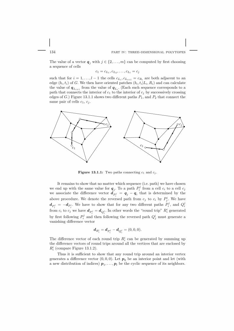
134 part iv: three-dimensional polytopes
The value of a vector qj with j ∈ 2, . . . ,m can be computed by first choosinga sequence of cells
c1 = cL1, cL2
, . . . , cLl= cj
such that for i = 1, . . . , l − 1 the cells cLi , cLi+1= cRi are both adjacent to an
edge (bi, ti) of G. We then have oriented patches (bi, ti|Li, Ri) and can calculatethe value of qLi+1
from the value of qLi. (Each such sequence corresponds to a
path that connects the interior of c1 to the interior of cj by successively crossingedges of G.) Figure 13.1.1 shows two different paths P1, and P2 that connect thesame pair of cells c1, cj .
c1
cj
c1
cj
Figure 13.1.1: Two paths connecting c1 and cj .
It remains to show that no matter which sequence (i.e. path) we have chosenwe end up with the same value for qj . To a path P j
i from a cell ci to a cell cjwe associate the difference vector dP j
i= qj − qi that is determined by the
above procedure. We denote the reversed path from cj to ci by P ij . We have
dP ji
= −dP ij. We have to show that for any two different paths P j
i , and Qji
from ci to cj we have dP ji
= dQji. In other words the “round trip” Ri
i generated
by first following P ji and then following the reversed path Qi
j must generate avanishing difference vector
dRii= dP j
i− dQj
i= (0, 0, 0).
The difference vector of each round trip Rii can be generated by summing up
the difference vectors of round trips around all the vertices that are enclosed byRi
i (compare Figure 13.1.2).
Thus it is sufficient to show that any round trip around an interior vertexgenerates a difference vector (0, 0, 0). Let p0 be an interior point and let (witha new distribution of indices) p1, . . . ,pl be the cyclic sequence of its neighbors.

3-polytopes 135
We get
∑li=1 ω0,i(p0 × pi) =
∑li=1 ω0,i((p0 × pi)− (p0 × p0))
=∑l
i=1 ω0,i(p0 × (pi − p0))
= p0 ×∑l
i=1 ω0,i(pi − p0)
= p0 × (0, 0, 0)
= (0, 0, 0)
The first equation holds since the p0 × p0 is always zero. The second and thirdequation hold by the linearity of the cross product. The fourth equation holdssince around every interior point we had an equilibrium.
Figure 13.1.2: A “round trip” is the sum of small cycles.
The vectors qi are now used to define a lifting function for the vectors qi.We define a piecewise linear function f :G → R from the convex hull of ourdrawing G = conv(pn−k, . . . ,pn) to R. This function f is defined by
f(x) = 〈x, qi〉 if x ∈ ci.
Lemma 13.1.2. The function f is well defined.
Proof. The only fact that we have to show is that for adjacent cells cL and cRthe functions 〈x, qL〉 and 〈x, qR〉 agree along the common edge e. Let (b, t|L,R)be the corresponding oriented patch. A point on the edge e can be written asp = λpb + (1 − λ)pt. Since the scalar product is linear it is sufficient to showthat the two functions agree on pb and pt.

136 part iv: three-dimensional polytopes
〈pb, qL〉 = 〈pb, ωb,t(pb × pt) + qR〉 = ωb,t〈pb, (pb × pt)〉+ 〈pb, qR〉 = 〈pb, qR〉.
A similar relation holds for pt.
The last lemma implies that f defines a unique height for each of the verticesp1, . . . ,pn. The following lemma shows that we have local convexity.
Lemma 13.1.3. For adjacent interior cells cL, and cR let ` be the line thatsupports the edge cL ∩ cR. Every point x that is on the same side of ` as qL
satisfies 〈x, qL〉 > 〈x, qR〉.
Proof. Let (b, t|L,R) be the corresponding oriented patch. We have
〈x, qL〉 − 〈x, qR〉 = 〈x, ωb,t(pb × pt)〉 = ωb,t · det(x,pb,pt) > 0,
by our orientation convention and the fact that the weight ωb,t is positive.
Finally, we prove global convexity by using Tutte’s Theorem.
Lemma 13.1.4. At a point x ∈ int(ci) the value 〈x, qi〉 is greater than allvalues 〈x, qj〉 with i 6= j.
Proof. To compare 〈x, qi〉 with some 〈x, qj〉, with j 6= i take a line ` thatconnects x with an interior point y of cj , such that ` does not path throughany of the points in P . Moving along ` from x to y defines (since by Tutte’sTheorem all cells are convex and decompose G) a sequence of cells
ci = cL1, cL2
, . . . , cLl= cj .
By Lemma 13.1.3 we have
〈x, qi〉 > 〈x, qL1〉 > 〈x, qL2
〉 > . . . > 〈x, qLl〉 = 〈x, qj〉.
This proves the claim.
Lemma 13.1.4 and Lemma 13.1.2 show that the set
X = x ∈ R3 | 〈x, qi〉 ≥ 0 for i = 1, . . . ,m ∩ (x, y, z) ∈ R
3 | (x, y, 1) ∈ G
forms an (unbounded) polyhedral set in the cylinder (x, y, z) ∈ R3 | (x, y, 1) ∈
G. Each of the equations 〈x, qi〉 = 0 supports a facet of X that projects to thecorresponding cell in our representation of G. The vertices of X are of the formp′i = (xi, yi, 〈pi, qj〉) where cj is a cell that contains the point pi = (xi, yi, 1). Itis not true that in general the lifted peripheral points p′n−k, . . . ,p
′n are automat-
ically coplanar. This is only the case if we can chose weights for the peripheraledges such that also the peripheral vertices are in equilibrium. However if the pe-ripheral cell is a triangle then the three lifted points are automatically coplanar.So we obtain immediately:

3-polytopes 137
Corollary 13.1.5. If a graph G is planar, 3-connected and contains a trian-gular cell, then it is the edge graph of a 3-polytope.
Proof. Chose the triangular cell as the peripheral polygon, chose positiveweights for the interior edges, find the equilibrium, and apply our lifting proce-dure. The resulting set X has to be intersected with a closed halfspace boundedby the plane that supports the lifted peripheral triangle in order to obtain thedesired polytope.
The last corollary is already the statement of Steinitz’s Theorem for thespecial case when G contains a triangle. The following considerations show howto proceed if this is not the case.
Lemma 13.1.6. A planar and 3-connected graph G contains either a triangularcell or a vertex of degree 3.
Proof. Let v, c, and e be the numbers of vertices, cells, and edges, respectively.Let αv be the average vertex degree and αc the average number of sides per cell.Since each edge is incident to exactly two vertices, we get αvv = 2e. Since eachedge is adjacent to exactly two cells, we get αcc = 2e. Adding these two equationsand inserting Euler’s formula we get:
αvv + αcc = 4e = 4v + 4c− 8.
This implies that at least one of the numbers αv or αc is less than 4. Since eachvertex degree is at least 3 and each cell has at least 3 sides, there is either atriangle or a vertex of degree 3.
The last lemma allows us to use polarity to prove the general Steinitz’sTheorem. If G is a 3-connected planar graph with cells c0, . . . , cm, then the polargraph G∆ of G is graph G∆ = (0, . . . ,m, E∆). The pair i, j is an edge inE∆ if ci and cj have an edge in common in G. The following lemma summarizesthe main properties of polarity of graphs and polytopes.
Lemma 13.1.7. Let P be a polytope and G be a 3-connected planar graph.
(i) G∆ is a 3-connected planar graph.
(ii) G∆∆ = G.
(iii) If G is the edge graph of P then G∆ is the edge graph of P ∆.
Proof. Proofs of these standard facts may be found in [65].

138 part iv: three-dimensional polytopes
We finally prove Steinitz’s Theorem.
Theorem 13.1.8 (Steinitz’s Theorem). If a graph G is planar and 3-connected, then it is the edge graph of a 3-polytope.
Proof. If G contains a triangular cell, then we are done by Corollary 13.1.5.Otherwise Lemma 13.1.6 implies that G has a vertex v of degree 3. In the polargraph G∆ this vertex corresponds to a triangular cell. Thus we can realize byCorollary 13.1.5 a polytope P ′ with edge graph G∆. Applying a translation, ifnecessary, we may assume that P ′ contains the origin in its interior. The polarP ′∆ has edge graph (G∆)∆ = G.
Example 13.1.9. This example demonstrates the different states of the con-struction for the case of a cube with one truncated vertex. The unique triangularcell is taken as the peripheral polygon. With the labels of Figure 13.1.3 the cellsare:
(2, 7, 9, 10, 5), (3, 5, 10, 8, 5), (4, 6, 8, 9, 7),
(1, 2, 5, 3), (1, 3, 6, 4), (1, 4, 7, 2), (8, 9, 10).
We set p8 = (0, 0), p9 = (1, 0), p10 = (0, 1), and chose the weights of the interioredges to be 1. The positions of the interior edges can then be calculated bysolving the equations M · x = bx and M · y = by. Here x = (x1, . . . , x7)
T andy = (y1, . . . , y7)
T are the x- and y-coordinates of the seven interior points. Thematrix M (the stress matrix) and the vectors bx and by are given by
M =
−3 1 1 1 0 0 01 −3 0 0 1 0 11 0 −3 0 1 1 01 0 0 −3 0 1 10 1 1 0 −3 0 00 0 1 1 0 −3 00 1 0 1 0 0 −3
; bx =
0000001
; bx =
0000100
.
Solving this system of linear equations and embedding the points in thez = 1 plane we get
p1 = ( 13 ,
13 , 1), p2 = ( 3
8 ,38 , 1), p3 = ( 1
4 ,38 , 1), p4 = ( 3
8 ,14 , 1),
p5 = ( 524 ,
712 , 1), p6 = ( 5
24 ,524 , 1), p7 = ( 7
12 ,524 , 1),

3-polytopes 139
=⇒1
2
3 4
5
6
7
8
9
10
c1
c2
c3
c4
c5
c6
1
23
4
5
6 7
8 9
10
Figure 13.1.3: A graph and its stressed embedding.
To calculate the heights of the points in a corresponding lifting we first haveto calculate the vectors q1, . . . , q6 that are associated to the cells. We get
q1 = (0, 0, 0)
q2 = q1 + p10 × p5 = ( 512 ,
524 ,− 5
24 )
q3 = q1 + p7 × p9 = ( 524 ,
512 ,− 5
24 )
q4 = q1 + p5 × p2 = ( 524 ,
16 ,− 9
64 )
q5 = q4 + p3 × p1 = ( 14 ,
14 ,− 35
192 )
q6 = q1 + p2 × p7 = ( 16 ,
524 ,− 9
64 )
It is easy to check that we get the same values independent from the particularsequences that we have chosen to calculate the qi. Now we get the heights byforming scalar products of the qi and the pv . We get
h1 = 〈p1, q4〉 = − 164 , h2 = 〈p2, q1〉 = 0,
h3 = 〈p3, q2〉 = − 5192 , h4 = 〈p4, q3〉 = − 5
192 ,
h5 = 〈p5, q1〉 = 0, h6 = 〈p6, q2〉 = − 564 ,
h7 = 〈p7, q1〉 = 0, h8 = 〈p8, q2〉 = − 524 ,
h9 = 〈p9, q1〉 = 0, h10 = 〈p10, q1〉 = 0.
Again it is easy to test the consistency of all possible ways to calculate the hi.If one prefers positive integers for the heights one can also multiply by a factorof −192 to obtain:
h1 = 3, h2 = 0, h3 = 5, h4 = 5, h5 = 0,
h6 = 15, h7 = 0, h8 = 40, h9 = 0, h10 = 0.

140 part iv: three-dimensional polytopes
13.2 A Quantitative Analysis
This section is devoted to the question of the size f(n) of a minimal grid1, 2, . . . , f(n)3 on which all combinatorial types of 3-polytopes with n verticescan be realized. Following the construction steps from a graph to a concretepolytope leads to an upper bound for this minimal grid size. The bound that weachieve will be singly exponential in n for the case of simplicial polytopes andit will be singly exponential in n2 for the general case. This improves the upperbound of n169n3
that was computed by Onn and Sturmfels [51]. We first calcu-late a bound for the case when the polytope P contains a triangle. For this wefirst compute an upper bound for the grid size that is needed for an equilibriumrepresentation of the edge graph of P .
Lemma 13.2.1. Let G be a planar 3-connected graph. G has at most 2|V | − 4cells. The average degree αv of the vertices of G is less than 6.
Proof. Let v, c, and e be the numbers of vertices, cells, and edges, respectively.Since c as well as αv is increased if we add edges to the graph we may assumethat all cells of G are triangles. Since all cells are triangles and each cell isadjacent to exactly 2 edges we have 2e = 3c. Combining this fact with Euler’sequation (v + c = e + 2) we get c = 2v − 4, which proves the first claim. Sinceeach edge is incident to exactly two vertices we have αv · v = 2e = 3c. Thus wehave αv · v = 6v − 12, and thus αv < 6.
Lemma 13.2.2. Let G be a 3-connected planar graph with a triangular cell c0and n vertices. There is an equilibrium embedding P of G on the integer grid0, 1, 2, . . . , (6.5)n−32.
Proof. Let G be a 3-connected planar graph with n vertices and with a trian-gular cell (n−2, n−1, n). We set k = n−3. We consider the equilibrium embed-ding in which all interior weights have been chosen to be 1. The triangular cellis chosen as peripheral polygon with coordinates pn−2 = (0, 0), pn−1 = (N, 0),pn = (0, N). Where N is a positive integer that will be determined later. Theequilibrium condition for the internal points pv = (xv , yv) is then written as
∑
v,w∈E
xv − xw = 0 and∑
v,w∈E
yv − yw = 0.
In matrix-form this can be written as M · x = bx and M · y = by. Here x =(x1, . . . , xk)T and y = (y1, . . . , yk)T . Let λv be the degree of the vertex v in G.The matrixM has size k×k. The v-th row of the matrixM contains an entry−λv
at position v (on the diagonal) and an entry 1 at positions w whenever v, wis an edge of G. All other entries are zero. The entry (bx)v is N if v, n − 1is an edge of G, and zero otherwise. Similarly, the entry (by)v is N if v, n isan edge of G, and zero otherwise. The matrix M is the stress-matrix of G. The

3-polytopes 141
values for x and y are by Tutte’s Theorem uniquely determined. This resultsin the fact that M has rank k. The value xv can be determined by Cramer’srule as xv = det(Mv)/det(M), where Mv is the obtained from M by replacingthe v-th column by bx. Since bx is N times an integer vector and all matrixentries are integers we get integral values for the xi if we chose N := det(M). Asimilar consideration holds for the values of y. All entries of x and y will thenbe integer numbers in the interval [0, N ], since all interior vertices are in theinterior of the peripheral triangle. Thus we have to find an upper bound for thevalue of det(M). This value can by Hadamard’s theorem be bounded by
det(M) ≤k∏
i=1
√(λ2
i + λi).
The term √(λ2
i + λi) = (λ2i + 12 + . . .+ 12
︸ ︷︷ ︸i times
)12
bounds the euclidean length of the i-th row vector of M from above, since thisvector has one entry −λi on the diagonal and at most λi entries of 1 elsewhere.By observing (λ2
i + λi) < (λi + 12 )2 and applying Lemma 13.2.1 we obtain the
chain of inequalities
det(M) ≤ ∏ki=1
√(λ2
i + λi) ≤∏k
i=1(λi + 12 ) ≤ (αv + 1
2 )k = (6.5)k.
The third inequality holds by the standard relation between the geometric andthe arithmetic mean.
The last lemma shows that we can embed equilibrium representations ingrids whose size is singly exponential in the number of vertices.
Remark 13.2.3. It is not clear at all whether one can find weights such thatonly a polynomial grid size is needed. If this were the case, this would be the keyto a polynomial upper bound for the grid size that is needed for 3-polytopes.
So far we have already determined the maximal size of the x-coordinatesand of the y-coordinates of a realization of the polytope that corresponds to G.We now have to study, how large the z-coordinate can get during our liftingprocess.
Lemma 13.2.4. Let P be a (combinatorial) 3-polytope that has a triangularfacet f0 and n vertices. There is a realization of P with integral vertex coordi-nates of absolute values less than 43n
Proof. Let P be the equilibrium representation from Lemma 13.3.2, of theedge graph of P . We assume that P is embedded in the plane z = 1. The zcoordinate to which a point pv is lifted is calculated by 〈pv , qj〉. Here qj is the

142 part iv: three-dimensional polytopes
vector that is associated to a cell cj that contains pv via Lemma 13.1.1. Thevector qj is calculated as the sum
qj =
l∑
i=1
(pbi× pti
).
Here (bi, ti|Li, Ri) is a sequence of oriented patches with L1 = 1, Rl = j, andRi = Li+1 for i = 1, . . . , l − 1. We need at most 2n − 4 summands since byLemma 13.2.1 the graph G has at most that many cells. Expanding 〈pv, qj〉 weget
〈pv, qj〉 = 〈pv ,l∑
i=1
(pbi× pti
)〉 =l∑
i=1
det(pv ,pbi,pti
).
Each of these determinants is an integer number of size at most ((6.5)n−3)2 (itcorrespond to twice the area of the triangle spanned by pv, pbi
, and pti.) Thus
we obtain〈pv , qj〉 ≤ ((6.5)n−3)2 · (2n− 4) < 43n
This Lemma already establishes the upper bound, if G contains a trianglefor the general case we have to analyze how the process of polarizing influencesthe vertex coordinates.
Lemma 13.2.5. Let P be a (combinatorial) polytope that has a triangular facetf0 and n vertices. There is a realization of P with integral vertex coordinates ofabsolute values less than 43n that contains the origin in its interior.
Proof. The bounding triangle is again realized by the homogenized pointspn−2 = (0, 0, 1), pn−1 = (N, 0, 1), pn = (0, N, 1), such that N is the deter-minant of the stress matrix. We choose the cell c1 as the interior cell adjacent tothe two points pn−1 and pn and apply the lifting construction. The coordinatebound is achieved by the last lemma. We now prove that the polytope that isgenerated contains a grid point in its interior. For this we reconstruct the vectorq0 that describes the lifting function of the exterior triangle c0. Let p1, . . . ,pl
be the interior points that are adjacent to pn, such that p1 is the point that iscontained in c1. The heights of the peripheral vertices are hn−2 = H , hn−1 = 0,hn = 0 with
H = 〈l∑
i=1
(pi×pn),pn−2〉 =
l∑
i=1
det(pi,pn,pn−2) =
l∑
i=1
det
xi 0 0yi N 01 1 1
> N.
The vector q0 such that hi = 〈q0,pi〉 for i = n−2, . . . , n is then uniquely givenby q0 = (−H
N ,−HN , H). The point p1 = (x1, y1, 1) is in c1 and therefor is lifted
to a height 0. Since p1 is interior we have x1 + x2 < N . Since x1 and x2 areintegers we even have N − x1 − x2 ≥ 1. On the other hand

3-polytopes 143
〈q0,p1〉 = −HNx1 −
H
Ny1 +H = H · N − x1 − x2
N≥ H
N≥ 1.
So, the ray that is vertically above (x1, y1, 0) contains a grid point g in P .Applying a translation that moves g to the origin gives the result.
Lemma 13.2.6. Let P be a polytope that has no triangular facet and n vertices.There is a realization of P with positive integral vertex coordinates of values lessthan 218n2
.
Proof. Let G be the edge graph of G and let G∆ be its polar. The graph G∆
contains a triangle. Thus we can apply Lemma 13.2.5 to G∆ and get a realizationP ∆ = (p0, . . . ,pm) of the polar of a realization of P . The hyperplanes thatsupport the faces f1, . . . , fn of this polytope that is generated in Lemma 13.2.5are of the form
Hi :=
(x, y, z) ∈ R3 | aix+ biy + ciz + 1 = 0.
(ai, bi, ci) for i = 1, . . . , n are the vertices of the desired realization P of P . Theycan be calculated by solving the system of equations aixij +biyij +cihij +1 = 0.
Here (xij , yij , hij ) for j = 1, . . . , 3 are the coordinates of points in P ∆ that lieon fi. Solving these equations by Cramer’s rule leads to coefficients ai, bi, andci of the form
det
∗ ∗ ∗∗ ∗ ∗1 1 1
/det
∗ ∗ ∗∗ ∗ ∗∗ ∗ ∗
.
Here ∗ are entries of absolute value less than 43n. The divisor is always identicalfor a fixed index i. The dividend and the divisor are of absolute value less than6 · 433n. Multiplying all points (ai, bi, ci) by the divisors of the remaining points,we can transform the rational coordinates into integral coordinates of absolutevalue less than (6 ·433n)n = (
√6 ·433)n2
< 194752n2
< 218n2
. The last inequalityis rough enough even to allow a translation that makes all coordinate entriespositive.
Summarizing the last two results we get:
Theorem 13.2.7.
• (i) All combinatorial types of 3-polytopes with n vertices can be realized on
an integer grid 0, 1, . . . , 218n2.• (ii) All combinatorial types of simplicial 3-polytopes with n vertices can be
realized on an integer grid 0, 1, . . . , 43n.
Remark 13.2.8. A slightly more careful analysis of the construction provesthat also a bound of 213n2
can be obtained for the coordinate size of general3-polytopes.

144 part iv: three-dimensional polytopes
13.3 The Structure of the Realization Space
In this section we finally prove that the structure of the realization space of a3-polytope is essentially trivial. If a polytope P has e edges the realization spaceR(P ) is an open ball of dimension e− 6. It is a remarkable fact that this resultwas already known to Steinitz (compare [56]). We will prove a slightly strongerresult that this realization space is in addition stably equivalent to 0 (i.e. it isa trivial semialgebraic set). We again restrict ourselves first to the case that P
contains a triangle. The general case is later proved by polarity arguments.
Let P be a 3-polytope with n vertices that contains a triangle p1,p2,p3,and let P be its combinatorial type. Furthermore, let p4 be another point of P
that is joined to p1 by an edge. Then (p1,p2,p3,p4) forms a basis for P . Weset e1 = (0, 0, 0), e2 = (1, 0, 0), e3 = (0, 1, 0), e4 = (0, 0, 1). For an arbitraryrealization P = (p1, . . . ,pn) of P we set pi = (xi, yi, hi). We will refer to theentry hi as the height of pi. We define
Rpos(P ) := P ∈ R3n | P realizes P and p1=e1, p2=e2, p3=e3, h4 > 0
R(P ) := P ∈ Rpos(P ) | p4=e4 Rlift(P ) := P ∈ Rpos(P ) | xi > 0, yi > 0, xi + yi < 0 for i = 4, . . . , n
We clearly have
R(P ) ⊆ R(P )pos and Rlift(P ) ⊆ Rpos(P ).
In all these definitions the points p1, p2, and p3 form a fixed triangle T =(e1, e2, e3) in the plane H = (x, y, h) ∈ R3 | h = 0. By abuse of language weuse the symbol T for both, the convex hull conv(T ) and for the set of its vertices.The space R(P ) is just the usual realization space as defined in Section 2. Herethe point p4 is fixed at the position e4. Rpos(P ) is a superset of R(P ). Thecondition for the position of p4 is relaxed. All points with positive heights areallowed. Hence Rpos(P ) consists of all realizations of P (with the fixed triangle)that lie in the closed halfspace H+ = (x, y, h) ∈ R
3 | h ≥ 0. The spaceRlift(P ) consists of all realizations in Rpos(P ) that project orthogonaly down tothe triangle T . Our first aim is to show that the spaceRlift(P ) corresponds to thespace of all realizations that are obtained by our self-stress/lifting constructions.It will be shown to be rationally equivalent to the space of all possible choicesof weights for the interior edges (with peripheral triangle T ). We assume that Phas e edges and set R
+ = x | x > 0.
Lemma 13.3.1. The space Rlift(P ) is rationally equivalent to (R+)e−3.
Proof. Let G be the edge graph of P . If we fix positive weights and realize Pby our self-stress/lifting construction with peripheral triangle T = (e1, e2, e3)we obtain a realization P that projects orthogonally onto the triangle T . Forgiven weights Ω ∈ (R+)e−3 let
P (Ω) = (p1(Ω), . . . ,pn(Ω)) ∈ R3n

3-polytopes 145
be the realization of P that comes from the self-stress/lifting construction. Weassume that the cell c1 corresponds to the facet that is adjacent to the facet(1, 2, 3) along the edge (1, 2). We furthermore assume that p4 belongs to thefacet c1. We then have p1(Ω) = (0, 0, 0), p2(Ω) = (1, 0, 0), p3 = (0, 1, h3(Ω)),and p3 = (x4(Ω), y4(Ω), 0) for all Ω ∈ (R+)e−3. The invertible rational functionfΩ(xi, yi, hi) := (xi, yi, hi) − (0, 0, yi · h3(Ω)) applied to each point associatesto every realization of the type P (Ω) a realization in Rlift(P ). Actually, fΩ isan affine transformation. We have to prove that g(Ω) = fΩ(P (Ω)) is a rationalequivalence between (R+)e−3 and Rlift(P ).
We first prove that P (Ω) is injective. Let Ω,Ω′ ∈ (R+)e−3 be two assign-ments of weights with P = P (Ω) = P (Ω′) = P ′. Both assignments of weightsgenerate identical equilibrium representations of the graphG. Assume that P hasfacets labeled by 0, . . . ,m with T corresponding to the index 0. Let q1, . . . , qm
be the facet vectors (as used in Section A.3) in the self-stress/lifting constructionfrom Ω and let q′1, . . . , q
′m be the corresponding vectors for Ω′. For any oriented
patch (b, t|L,R) we have
ωb,t(pb × pt) = qL − qR = q′L − q′R = ω′b,t(pb × pt).
This implies Ω = Ω′. If g(Ω) = g(Ω′) we must have in particular P (Ω) = P (Ω′),which proves that G is injective.
We now prove the existence of a rational inverse g−1 of g. We do thisby determining a rational construction that associates to every polytope P ′ inRlift(P ) a choice of positive weights Ω with g(Ω) = P ′. We do this by justreversing our construction (actually this is in principle the construction thatwas already known to Maxwell more than 100 years ago).We first apply an affinetransformation that leaves p′1, and p′2 invariant and moves p′4 = (x4, y4, h4) intothe position (x4, y4, 0). The resulting polytope is called P . The projection ofthe edge skeleton of P to T is a planar representation of G with boundary T .By p∗i we denote the point (xi, yi, 1) (the homogenization of the projection ofpi.) To each facet fi we associate the corresponding cell ci, and determine the(unique) vector qi such that (x, y) 7→ 〈(x, y, 1), qi〉 describes the lifting functionfrom ci to fi in the realization P . We obtain our weights Ω by assigning toeach each oriented patch (b, t|L,R) a weight ωb,t by qL − qR = ωb,t(p
∗b × p∗t ).
This is possible since qL − qR is a scalar multiple of p∗b × p∗t , since the liftingfunctions for fL and fR agree on the points p∗b and p∗t (compare the calculationof Lemma 13.1.1). Reversing the argumentation of Lemma 13.1.2 we see thatwe have equilibrium around every interior vertex. Reversing the argumentationof Lemma 13.1.3 shows that the convexity of P translates to the fact that theweights are positive.
We now compare the spaces Rlift(P ) and R(P ). Let P = (p1, . . . ,pn) ∈R(P ) be a realization of P . For i = 1, . . . , n we set phom
i = (xi, yi, hi, 1) — thehomogenization of pi.
A projective transformation of the points in P may be expressed by mul-tiplying P hom by a non-degenerate 4 × 4 matrix and then dehomogenizing by

146 part iv: three-dimensional polytopes
dividing by the 4-th coordinate. If z 6= 0, we denote this process of dehomog-enization by (x, y, h, z)dehom = (x/z, y/z, h/z). We consider a class of specialprojective transformations
τa,b,c =
1 0 a 00 1 b 00 0 1 00 0 c 1
.
All such transformations τa,b,c leave the plane H = (x, y, 0) ∈ R3 invariant.
The determinant of the transformation matrix is 1, thus the transformationspreserve orientation. We consider the set
R∗(P ) :=(τa,b,c(P
hom))dehom | a, b, c ∈ R; P ∈ R(P ) and
〈τa,b,c(phomi ), (0, 0, 0, 1)〉 > 0, 〈τa,b,c(p
homi ), (1, 0, 0, 0)〉 > 0,
〈τa,b,c(phomi ), (0, 1, 0, 0)〉 > 0, 〈τa,b,c(p
homi ), (−1,−1, 0, 1)〉 > 0;
for i = 4, . . . , n.
The dehomogenization is always possible since the z-coordinate is forced to bepositive by the first inequality. The other three inequalities encode the conditionthat for P ∈ R∗(P ) the points p4, . . . ,pn project orthogonally to T .
Lemma 13.3.2.
(i) R∗(P ) ≈ R(P ),
(ii) dim(R∗(P )) = dim(R(P )) + 3,
(iii) R∗(P ) = Rlift(P ).
Proof. By A(P ) we denote the set of all (a, b, c) that are admissible for thechoice of τa,b,d for given P in the definition of R∗(P ). This set is bounded by4(n−4) linear equations. We have τa,b,d(xi, yi, hi, 1) = (xi +hia, yi +hib, hi, 1+hic). The set A(P ) is never empty, since for sufficiently large λ > 0 the vectorλ(1/3, 1/3, 1) = (a, b, c) satisfies all inequalities (since the hi are all positive).Hence, the set R(P ) is a stable projection of the set
R(P ) := (P , (a, b, c)) | P ∈ R(P ) and (a, b, c) ∈ A(P ).
The dimension ofR(P ) is dim(R(P ))+3. Performing the projective transforma-tion and the dehomogenization is an invertible rational operation. Thus R(P )and R∗(P ) are rationally equivalent. This proves (i) and (ii).
By definition we have R∗(P ) ⊆ Rlift(P ). To see R∗(P ) ⊇ Rlift(P ) We mustfind for every P ∈ Rlift(P ) a P ′ ∈ R(P ) and an admissible (a, b, c) ∈ A(P )such that (τa,b,c(P
hom))dehom = P . For P ∈ Rlift(P ) with p4 = (x4, y4, h4) weset (a, b, c) = (x4/h4, y4/h4, (1/h4 − 1)). We then have

3-polytopes 147
(τa,b,c(ehom4 ))dehom = (τa,b,c(0, 0, 1, 1))dehom
= (x4/h4, y4/h4, 1, 1/h4)dehom
= (x4, y4, h4).
We finally set P ′ = (τa,b,c)−1(P ). The polytope P ′ is the desired element from
R(P ). This proves (iii)
Combining Lemma 13.3.1 and Lemma 13.3.2 we get.
Theorem 13.3.3. For a 3-polytope P with e edges the realization space R(P )is an open ball of dimension e− 6. R(P ) is a trivial semialgebraic set.
Proof. If P contains a triangle we can apply Lemma 13.3.1 and Lemma 13.3.2.The dimension count is dim(R(P )) = dim(Rlift(P )) − 3 = e− 6 Since R(P ) ≈Rlift(P ) ≈ (R+)e−6 ≈ 0 the space R(P ) is trivial.
If P does not contain a triangle then by Lemma 13.1.6 it has a vertex ofdegree 3. Then P∆ contains a triangle. Theorem 2.6.3 states that the realizationspaces of P and P∆ are stably equivalent and have the same dimension.

148 part iv: three-dimensional polytopes
Part V: Alternative Construction Techniques
During the process of “cooking up” the proof of the Universality Theorem manynice constructions were explored that are of interest on their own right. It is thepurpose of this part to sketch the two most beautiful such constructions. Bothlead to weaker results than the Universality Theorem as proved in the main partof this monograph. However in both cases the construction relies on structuralproperties of polytopes that are different from the tools that have been usedthere.
The first construction provides a class of polytopes that prove a Non-SteinitzTheorem in dimension 5. It makes use of Ziegler’s example of a 5-polytope con-taining a hexagon all whose vertices must lie on a conic. Many copies of Ziegler’sexample are glued in a completely symmetric way along a polytope that en-codes an incidence theorem concerning conics. Local perturbations in this classof examples gives the desired class of combinatorial polytopes.
The second construction leads to a Universality Theorem for polytopes indimension six. It establishes a relatively simple and symmetric way to use Mnev’sUniversality Theorem for oriented matroids as a starting point that can be trans-lated into a corresponding theorem for polytopes. This construction makes useof the fact that realizable oriented matroids correspond to zonotopes (a specialclass of polytopes).
14 Generalized Adapter Techniques
Before we go into the details of the “alternative constructions,” we discuss amethod that makes their description a bit easier. When we introduced our Ba-sic Building Block “transmitter for line slopes” in Section 5.7, we were facedwith the problem of gluing polytopes along facets that were not combinatoriallyequivalent. We solved this problem by inserting intermediate polytopes called“adapters” (compare Section 5.5). This method also works in more general set-tings. We will make use of this refined method in the following two sections.
Recall that every face of a combinatorial d-polytope is characterized by itsvertex set. For a k1-face F k1 and a k2-face F k2 of a combinatorial d-polytopewith 0 ≤ k1 < k2 ≤ d we have F k1 ⊂ F k2 if F k1 is a proper face of F k2 . Let P d
and Qd be two (combinatorial) d-polytopes and let F k be a k-face that occurs
in both polytopes P and Q. Our aim is to find a polytope P d∼
#F k Qd that
149

150 part v: alternative construction techniques
contains the polytopes P d and Qd as summands of connected sums, such thatthey are identified along the face F k. Let
F k = F kP ⊂ F k+1
P ⊂ . . . ⊂ F dP = P d
be a maximal chain of faces in P and let
F k = F kQ ⊂ F k+1
Q ⊂ . . . ⊂ F dQ = Qd
be a maximal chain of faces in Q. Furthermore, assume that F d−1P and F d−1
Q
are necessarily flat. By pyri(F ) we denote the i-times iterated pyramid over F(the polytope pyr3(F ) is the pyramid of the pyramid of the pyramid of F ; thepolytope pyr0(F ) is F itself). Consider the combinatorial polytopes
P ij = pyrj(F
iP ) and Qi
j = pyrj(FiQ)
for i = k, . . . , d and j = 0, . . . , d−k. P ij is the j-times iterated pyramid over F i
P .
In particular, P i0 = F i
P and P d0 = P . P i
d−i is a d-polytope. The combinatorial
polytope P id−i contains P i
d−i−1 (for i = d−1, . . . , k) and P i−1d−i (for i = d, . . . , k+1)
as facets. A similar statement holds for the polytopes Qij . We also have P k
d−k−1 =
Qkd−k−1. All these polytopes of the types P i
d−i−1 or Qid−i−1 are necessarily flat
(either they are pyramids or they are F d−1P or F d−1
Q ). We can generate the desired
polytope P d∼
#F k Qd by forming a chain of connected sums as indicated by thefollowing construction diagram. Although the construction depends on the chains
of facets that have been chosen, we use the ambiguous notation P d∼
#F k Qd.
P d0
P d−1
1P d−2
2P k+1
d−k−1
P d−1
0P d−2
1P d−3
2 . . . P k+1
d−k
P kd−k−1
Qd0 Qd−1
1Qd−2
2Qk+1
d−k−1
Qd−1
0Qd−2
1Qd−3
2 . . . Qk+1
d−k
Iterative application of Lemma 3.2.4 shows
Lemma 14.1.1. Let R = P∼
#F Q and let P and Q be realizations of com-binatorial d-polytopes P and Q, respectively. If the face P
∣∣F
is projectively
equivalent to the face Q∣∣F, then there exists a projective transformation τ such
that conv(P ∪ τ(Q)) is a realization of R.

a non-steinitz theorem in dimension five 151
15 A Non-Steinitz Theorem in Dimension Five
The construction presented here provides a proof that there is no local character-ization for boundary complexes of 5-polytopes. (This construction was the originof the further investigations that led to the complete Universality Theorem.)The construction proceeds as follows:
• First we provide a class of incidence theorems of the following form: Letp1, . . . ,pk be a collection of points in R
d. If for a certain collection of 6-tuples the points in each 6-tuple are coplanar and lie on a conic, then an-other 6-tuple of points also lies on a conic. All the points involved lie onthe edge skeleton of an embedded, triangulated, orientable 2-manifold M .Exactly two of the points lie on each edge of M . The 6-tuples of pointsunder consideration are those coming from faces of M .
• We embed a certain class of such manifolds Mn (n = 6, 8, 10 . . .) in 4-polytopes and perform a truncation operation such that the vertices of theincidence theorem become vertices of a polytope P Mn . This polytope P Mn
contains n hexagonal 2-faces H1, . . . ,Hn. All realizations P of P Mn sharethe following property: If the six vertices of each H1, . . . ,Hn−1 lie on aconic then the vertices of Hn lie on a conic as well.
• Finally, we consider the pyramid P ′Mn over P Mn (a 5-dimensional poly-
tope). Along each of the hexagons Hi for i = 1, . . . , n − 1 we glue (usingconnected sums, and generalized adapter techniques) a copy of Ziegler’spolytope P Z (as described in Example 3.4.3), which forces the vertices ofHi to lie on a conic. Along Hn we (combinatorially) glue a copy of a per-turbed version P ′
Z of P Z that forces the vertices of Hn not to lie on aconic.
• The resulting (combinatorial) polytope is not realizable, since on the onehand the vertices ofHn must lie on a conic (as a consequence of the incidencetheorem), and on the other hand they cannot lie on a conic, since theymust satisfy the condition forced by P ′
Z. However, the global constructionis responsible for the non-realizability. If we delete one of the (essential)points then we can complete the remainder of the face lattice to a realizablepolytope. This provides a Non-Steinitz Theorem !
15.1 Conics and Incidence Theorems
We start with some considerations about conics in the plane. Conics are anintrinsically projective concept, therefore it is convenient to study them usinghomogeneous coordinates.
Definition 15.1.1. Let λ1, . . . , λ6 ∈ R be six real numbers at least one ofwhich is non-zero. The set (x, y, z) ∈ C3 | λ1x
2 + λ2y2 + λ3z
2 + λ4yz + λ5xz +λ6xy = 0 is a quadratic cone.

152 part v: alternative construction techniques
In other words, a quadratic cone is an algebraic set that is obtained bysolving a single homogeneous quadratic equation. The set of solutions may haveno non-zero real solutions at all (for instance consider the equation x2+y2+z2 =0). However, we will be interested only in the real part of the solution. If aquadratic equation can be written as the product of two real linear factors, thenthe corresponding quadratic cone degenerates into two linear hyperplanes (whichmay even coincide). If we dehomogenize a real non-degenerate quadratic cone byintersecting with an affine hyperplane H we obtain a planar conic. Dependingon the position of H , we get either an ellipse, a parabola, or a hyperbola.
Lemma 15.1.2. Let (x1, y1, z1), . . . , (x6, y6, z6) ∈ R3 be homogeneous coordi-nates for six planar points. The points lie on a common conic if and only if
C(1, 2, 3, 4, 5, 6) := det
x21 y2
1 z21 y1z1 x1z1 x1y1
x22 y2
2 z22 y2z2 x2z2 x2y2
x23 y2
3 z23 y3z3 x3z3 x3y3
x24 y2
4 z24 y4z4 x4z4 x4y4
x25 y2
5 z25 y5z5 x5z5 x5y5
x26 y2
6 z26 y6z6 x6z6 x6y6
= 0.
Proof. A point with homogeneous coordinates (x, y, z) is on a conic with pa-rameters λ1, . . . , λ6 if (x, y, z) satisfies the corresponding equation from Defini-tion 15.1.1. Thus six points (x1, y1, z1), . . . , (x6, y6, z6) are on a common conicif and only if there are parameters λ1, . . . , λ6 such that all (xi, yi, zi) satisfy thecorresponding quadratic equation. We may write the quadratic equations as thescalar product
〈(λ1, . . . , λ6), (x2i , y
2i , z
2i , yizi, xizi, xiyi)〉 = 0
of the parameters with the quadratic coordinates. Thus there is a set of param-eters as desired if and only if the quadratic coordinates are linearly dependent.This happens if and only if the determinant in the lemma vanishes.
We now switch to the special case, in which the cutting hyperplane ofhomogenization/dehomogenization chosen isH = (x, y, z) ∈ R3 | x+y+z = 1.Furthermore, we assume that the six points x1, . . . ,x6 are chosen on the sides ofthe triangle (e1, e2, e3) = ((1, 0, 0), (0, 1, 0), (0, 0, 1)) – two points on each side.By this (in homogeneous coordinates) each of the points x1, . . . ,x6 has at leastone zero entry. We furthermore assume that no two points coincide. The specialchoice of coordinates is not a serious restriction since any situation can be trans-formed to this special case by a change of coordinate system. The determinantof the last lemma becomes much simpler and factors nicely. For the labeling ofthe coordinates in the following Lemma we refer to Figure 15.1.1.

a non-steinitz theorem in dimension five 153
Lemma 15.1.3. Six mutually distinct points x1, . . . ,x6 ∈ R3 on the edges of a
triangle (e1, e2, e3) — as in Figure 15.1.1 — are on a conic if and only if
a2b2c2d2e2f2 − a1b1c1d1e1f1 = 0.
Proof. With our special choice of coordinates, the condition of Lemma 15.1.2translates to:
C(1, . . . , 6) = det
a21 a2
2 0 0 0 a1a2
b21 b22 0 0 0 b1b20 c21 c22 c1c2 0 00 d2
1 d22 d1d2 0 0
e22 0 e21 0 e1e2 0f22 0 f2
1 0 f1f2 0
= (a1b2−a2b1)(c1d2−c2d1)(e1f2−e2f1)(a2b2c2d2e2f2−a1b1c1d1e1f1).
Since the points x1, . . . ,x6 are all distinct, the first three factors (actually 2× 2determinants that indicate whether the two points on an edge are identical) areall non-zero. Therefore the entire expression is zero if and only if the last factoris zero.
e1 = (1, 0, 0)
e2 = (0, 1, 0) e3 = (0, 0, 1)
x1 = (a1, a2, 0)
x2 = (b1, b2, 0)
x3 = (0, c1, c2) x4 = (0, d1, d2)
x5 = (e2, 0, e1)
x6 = (f2, 0, f1)
Figure 15.1.1: Six points on the edges of triangle that lie on a conic.
We end with another more euclidean characterization for six points on aconic. The characterization follows directly from Lemma 15.1.3. We introducesome notation, which will also be needed later.
Let x and y be the endpoints of an (oriented) line segment s = (x,y) andp be a point on s. We define
rs(p) :=||y,p||||x,p|| ,
where ||a, b|| denotes the oriented euclidean distance between a and b.

154 part v: alternative construction techniques
Lemma 15.1.4. Let (q1, q2, q3) be the vertices of a planar triangle T with twoadditional points ai, bi on each of the sides si = (qi, qi+1), with indices modulo3. Assume that the points are pairwise distinct. The points a1, b1,a2, b2,a3, b3
are on a conic if and only if
rs1(a1) · rs1
(b1) · rs2(a2) · rs2
(b2) · rs3(a3) · rs3
(b3) = 1.
Proof. After a suitable affine transformation, which does not change the valueof the functions r( . . . ), we may assume that T is an equilateral triangle. If weuse the hyperplane H = (x, y, z) | x + y + z = 1 for the homogenization, wemay represent the vertices q1, q2, q3 by unit vectors e1, e2, e3 ∈ R
3, respectively.Homogeneous coordinates for the points ai and bi are then given by
a1
b1
a2
b2
a3
b3
=
rs1(a1) 1 0
rs1(b1) 1 00 rs2
(a2) 10 rs2
(b2) 11 0 rs3
(a3)1 0 rs3
(b3)
.
The condition in Lemma 15.1.3 translates to:
rs1(a1) · rs1
(b1) · rs2(a2) · rs2
(b2) · rs3(a3) · rs3
(b3) = 1
This proves the lemma.
Using this characterization we now prove an incidence theorem concerningconics on 2-manifolds.
Definition 15.1.5. Let M be an oriented simplicial 2-manifold with (triangu-lar) 2-faces f1, . . . , fn, edges e1, . . . , em and vertex set V = (q1, . . . , ql) ∈ R
d·l.Let P := a1, . . . ,am, b1, . . . , bm be distinct additional points such that ai
and bi lie on the edge ei for i = 1, . . . ,m. Such a manifold together with theadditional points ai, bi in the specified order will be called an ab-manifold M .
For each 2-face fi there are exactly six such additional points in P incidentwith fi. They will be called the hexagon of fi.
Theorem 15.1.6. Let M be an ab-manifold and for i = 1, . . . , n let Hi be thehexagon of fi. If for i = 1, . . . , n − 1 the vertices of Hi lie on a conic, then thevertices of Hn lie also on a conic.
Proof. Let M be the ab-manifold equipped with a consistent orientation onthe faces (for each edge the adjacent triangles should induce opposite orien-tations). For a triangle fi we assume that (qi,1, qi,2, qi,3) are its vertices or-dered consistently with the given orientation. We get a set of three oriented

a non-steinitz theorem in dimension five 155
edges Ei := (qi,1, qi,2), (qi,2, qi,3), (qi,3, qi,1) around the face fi. If two 2-faces fi1 and fi2 have two vertices x,y in common and s = (x,y) ∈ Ei1 thens = (y,x) ∈ Ei2 . By as and bs we denote the two points that lie on the edge s.We have
rs(as) = rs(as)−1 and rs(bs) = rs(bs)
−1.
This impliesn∏
i=1
∏
s∈Ei
(rs(as) · rs(bs)) = 1,
since each of the edges is used exactly once in both possible orientations. If fori = 1, . . . , n− 1 the vertices of Hi lie on a conic, then we have
∏
s∈Ei
(rs(as) · rs(bs)) = 1,
for i = 1, . . . , n−1, by Lemma 15.1.4. Combining these equations with the aboveexpression gives ∏
s∈En
(rs(as) · rs(bs)) = 1.
Thus the points of Hn are on a conic, by Lemma 15.1.4.
Figure 15.1.2 (a) shows part of a typical ab-manifold. Figure 15.1.2 (b)shows the same part of the ab-manifold together with some of the conics thatare relevant for Theorem 15.1.6.
(a) (b)
Figure 15.1.2: Part of an ab-manifold, with and without conics.
The smallest case of this theorem, where M is the boundary of a tetrahedron,is illustrated in Figure 15.1.3. If for three facets of the tetrahedron the verticesof the hexagon lie on a conic, then this is also the case for the last facet.

156 part v: alternative construction techniques
Figure 15.1.3: An incidence theorem on the boundary of a tetrahedron.
15.2 An Incidence Theorem for 4-Polytopes
Our last theorem indicates how to encode incidence theorems about conics intothe boundary of a polytope. Unfortunately Theorem 15.1.6 tells us nothing aboutthe shape of specific hexagonal faces of a polytope, since the vertices ai, bi arenot vertices of the underlying manifold. We now provide one special class of4-polytopes (P n)n≥3 that realize incidence theorems on hexagonal 2-faces. Thepolytope P n contains m = 2n hexagonal 2-faces with the property that co-conicality of the vertices of m− 1 hexagons implies co-conicality of the last one.Actually there are many ways of constructing such polytopes. For later use wepick out one special class which satisfies certain additional symmetry properties.
We start by describing these polytopes by explicit (homogeneous) coordi-nates. For n ≥ 3 the polytope P n has 6n+ 2 vertices. To construct P n we startwith the vertices
pn(i) = (1, cos(2iπ
n), sin(
2iπ
n), 0, 0) for i = 1, . . . , n
of a regular convex n-gon (embedded by homogeneous coordinates in R5). Fur-
thermore we need the vertices x′ = (1, 0, 0, 1, 0) and y′ = (1, 0, 0, 0, 1). All thesevertices lie on the linear hyperplane H = x ∈ R5 | x1 = 1. Thus the verticesspan a positive cone. Cutting this cone with the hyperplane H gives us a convexpolytope P n
A. In what follows we will identify the vertices of the polytopes withtheir homogeneous coordinates. The transition from homogeneous coordinatesof a vertex v to the vertex can be always made by cutting the positive span R
+v
with the hyperplane H .

a non-steinitz theorem in dimension five 157
For fixed n the convex hull of the vertices pn(1), . . . ,pn(n),x′,y′ forms apyramid over the pyramid over an n-gon. The 3-faces of P n
A are two pyramidsover an n-gon
(pn(1) . . .pn(n),x′
),
(pn(1) . . .pn(n),y′
)
and a ring of n tetrahedra(pn(i),pn(i+ 1),x′,y′
).
We now take this polytope P nA and “truncate” each single vertex v. We can
do this by replacing the vertex v (of edge-degree k) by k vertices v1, . . . ,vk ona hyperplane such that the new vertices are close to v and lie on the k edgesthat are incident with v. This truncation corresponds to the intersection of thepolytope P n
A with a halfspace that contains all vertices except for v. By trun-cating all vertices we generate a polytope that has two points on each edge ofP n
A. Actually, in our case we can make the “close to” part of this constructionvery rough. For an edge (v1,v2) the point “close to” v1 will be chosen at ho-mogeneous coordinates 2v1 + v2. The resulting polytope P n has the followingvertices:
an(i) = 2pn(i) + pn(i+ 1), bn(i) = pn(i) + 2pn(i+ 1),
cn(i) = 2pn(i) + x′, dn(i) = pn(i) + 2x′,
en(i) = 2pn(i) + y′, fn(i) = pn(i) + 2y′,
for i = 1, . . . , n, and the two vertices
x = 2x′ + y′, y = 2y′ + x′.
The vertices (dn(1) . . .dn(n),x) are those close to our original point x′. They alllie on the hyperplane (x1, . . . , x5) ∈ R
5 | 2x1 = 3x4, and form a facet whichis a pyramid over an n-gon. The vertices (fn(1) . . .fn(n),y) are the verticesclose to our original point y′. The vertices close to the original point pn(i) are(an(i), bn(i − 1), cn(i), en(i)), where indices are taken modulo n. These facetsare tetrahedra.
The remaining facets of P n have the vertex sets:
Xn =(x, cn(1) . . . cn(n),dn(1) . . .dn(n),an(1) . . .an(n), bn(1) . . . bn(n)
),
Yn =(y, en(1) . . .en(n),fn(1) . . .fn(n),an(1) . . .an(n), bn(1) . . . bn(n)
),
Tn(i) =(x,y,an(i), bn(i), cn(i), cn(i+ 1),dn(i),dn(i+ 1),
en(i), en(i+ 1),fn(i),fn(i+ 1)).
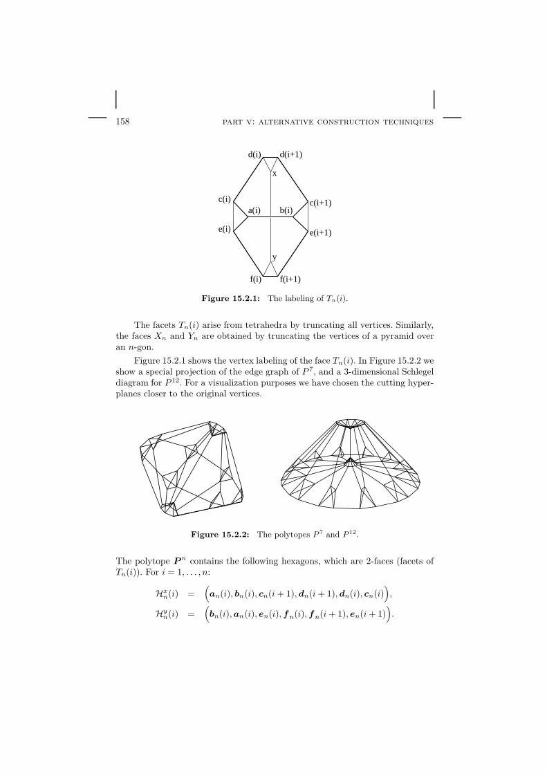
158 part v: alternative construction techniques
f(i) f(i+1)
e(i+1)
c(i+1)
d(i+1)d(i)
x
y
b(i)a(i)c(i)
e(i)
Figure 15.2.1: The labeling of Tn(i).
The facets Tn(i) arise from tetrahedra by truncating all vertices. Similarly,the faces Xn and Yn are obtained by truncating the vertices of a pyramid overan n-gon.
Figure 15.2.1 shows the vertex labeling of the face Tn(i). In Figure 15.2.2 weshow a special projection of the edge graph of P 7, and a 3-dimensional Schlegeldiagram for P 12. For a visualization purposes we have chosen the cutting hyper-planes closer to the original vertices.
Figure 15.2.2: The polytopes P 7 and P 12.
The polytope P n contains the following hexagons, which are 2-faces (facets ofTn(i)). For i = 1, . . . , n:
Hxn(i) =
(an(i), bn(i), cn(i+ 1),dn(i+ 1),dn(i), cn(i)
),
Hyn(i) =
(bn(i),an(i), en(i),fn(i),fn(i+ 1), en(i+ 1)
).

a non-steinitz theorem in dimension five 159
Theorem 15.2.1. For n ≥ 3 let P be a polytope combinatorially equivalentto P n. If the points of the hexagons Hx
n(1), . . . ,Hxn(n),Hy
n(1), . . . ,Hyn(n−1) are
on a conic then the points of Hyn(n) are also on a conic.
Proof. The main idea of the proof is to take a realization P of P n and toreconstruct the original points before the truncation. Then we consider a certainsubstructure of P n
A together with the vertices of P n as an ab-manifold and applyTheorem 15.1.6.
Let P be any realization of P n. During this proof we label the vertices andfaces of P by the letters a(i), b(i), c(i),d(i), e(i),f(i),x,y, T (i), X, Y consistentwith our original labeling of the vertices of P n. The hyperplanes supporting thefaces T (i), T (i+ 1), X, Y of P meet in a common point p(i). In particular, thepoint p(i) lies on the support of the edges
T (i) ∩X ∩ Y = (a(i), b(i)),
T (i+ 1) ∩X ∩ Y = (a(i+ 1), b(i+ 1)),
T (i) ∩ T (i+ 1) ∩X = (c(i),d(i)),
T (i) ∩ T (i+ 1) ∩ Y = (e(i),f(i)).
Furthermore the supports of all 3-faces T (1), . . . , T (n) meet in a line, since these3-faces share the edge (x,y). Hence the supports of the faces T (1), . . . , T (n), Xmeet in one point x′, which lies on all the supports of all edges (c(i),d(i)) fori = 1, . . . , n. Similarly, all faces T (1), . . . , T (n), Y meet in one point y′, whichlies on all the supports of all edges (e(i),f(i)) for i = 1, . . . , n. Now consider theoriented 2-manifold M that is formed by the vertices
p(1), . . . ,p(n),x′,y′
and the (oriented) triangles(p(i),p(i+ 1),x′
)and
(p(i+ 1),p(i),y′
)
for i = 1, . . . , n, indices counted modulo n. Actually, M has the combinatorialtype of a double pyramid over an n-gon. Together with our vertices
a(i), b(i), c(i),d(i), e(i),f(i)
for i = 1, . . . , n, which lie on the edges of M , the manifold M forms an ab-manifold with hexagons Hx(i), and Hy(i), for i = 1, . . . , n. Theorem 15.1.6proves the desired result.
Lemma 15.2.2. The special realization P n realizes the case, in which the ver-tices of each hexagon Hx
n(i) and Hyn(i) lie on a conic.
Proof. The result is clear by the symmetry of the chosen coordinates. We couldalso prove this fact by explicitly using the criterion of Lemma 15.1.5.

160 part v: alternative construction techniques
15.3 The Non-Steinitz Theorem
Combining the polytopes P n with Ziegler’s polytope P Z that forces six pointsto lie on a conic, we are almost done. We recall the properties of the 5-polytopeP Z (compare Example 3.4.3).
• P Z contains a hexagonal 2-face H,
• in every realization of P Z the vertices of H are on a conic,
• every hexagon whose vertices are on a conic can be completed to a realiza-tion of P Z.
Recall that P Z was constructed as a three-fold Lawrence extension over a draw-ing of Pascal’s Theorem (compare Figure 3.4.3). To emphasize the symmetricstructure of P Z we also give here a set of “nice” homogeneous coordinates for arealization and the vertex/facet incidence table.
2 1 0 0 0 01 2 0 0 0 00 2 1 0 0 00 1 2 0 0 01 0 2 0 0 02 0 1 0 0 01 0 0 1 0 00 1 0 0 1 00 0 1 0 0 10 0 1 1 0 01 0 0 0 1 00 1 0 0 0 1
f0 f1 f2 f3 f4 f5 f6 f7 f8 f9
z1 × × × × ×z2 × × × × ×z3 × × × × ×z4 × × × × ×z5 × × × × ×z6 × × × × ×
z7 × × × × × × ×z8 × × × × × × ×z9 × × × × × × ×
z10 × × × × × × ×z11 × × × × × × ×z12 × × × × × × ×
We obtain a perturbed version P ′Z of P Z if we start with a hexagon whose
points do not lie on a conic. The six points of the Lawrence extensions are then nolonger on a single facet. The facet f0 of P Z is then broken into three tetrahedra.This is the only change in the face lattice.
We relabel the hexagons of P n that are involved in our construction by
F1 = Hxn(1), . . . , Fn = Hx
n(n), Fn+1 = Hyn(1), . . . , F2n = Hy
n(n).
Using the generalized adaptor techniques from Section 14 we perform connectedsums that glue to each of the hexagons F1, . . . , F2n−1 a copy of the polytope P Z.Along F2n = Hy
n(n) we glue the perturbed polytope P ′Z. We call the resulting
(combinatorial) polytope P nR . The 2n − 1 copies of P Z are P 1
Z . . .P2n−1Z . The
vertices of each of these copies has to be relabeled properly to fit to the corre-sponding hexagon Fi. Formally we may write
PnR = P n
∼
#F1P 1
Z
∼
#F2. . .
∼
#F2n−1P 2n−1
Z
∼
#F2nP ′
Z.

a non-steinitz theorem in dimension five 161
Theorem 15.3.1.
(i) PnR is not polytopal.
(ii) Every minor of P nR can be completed to a polytopal face lattice.
Proof. For part (i) assume that there is a realization P of P nR . In P all the
hexagons Hxn(1), . . . ,Hx
n(n),Hyn(1), . . . ,Hy
n(n−1) have their vertices on a conic,since they are part of the summands P i
Z. By Theorem 15.2.1 this implies that thevertices of Hy
n(n) are on a conic, since all the hexagons are part of the summandP n. This contradicts the fact that this hexagon is part of the summand P ′
Z,which forces the vertices not to lie on a conic.
Part (ii) of this theorem (the minor minimality) is really technical. We omitit here. In principle it is a consequence of the fact that the non-realizability ofPn
R is forced by the global structure of the face lattice. Each point contributesto the non-realizability. Deleting any point allows us to find a realization of theremaining part of the face lattice that can be completed to a polytope.

162 part v: alternative construction techniques
16 The Universality Theorem in Dimension 6
In the main part of this monograph we proved the Universality Theorem for 4-polytopes “from scratch”. We gave explicit constructions that model multiplica-tion and addition on the level of realizations of polytopes. In contrast to that, fora long time it was believed that the easiest approach to a Universality Theoremfor polytopes in fixed dimension must be based on oriented matroids. As previ-ously mentioned, Mnev proved (already in 1986) the Universality Theorem fororiented matroids [49, 52] (we presented a relatively simple proof of this theorem“en passant” in Section 11.7). Mnev used his Universality Theorem combinedwith Gale Diagram techniques to prove a Universality Theorem for polytopeswithout a fixed bound on the dimension (compare Section 3). To prove sucha theorem for fixed dimension d, all that was missing, one thought, was someconstruction that associates to a given oriented matroidM a d-polytope P (M),for some fixed d, such that the realization spaces of M and P (M) are stablyequivalent. Here we present such a construction. Unfortunately, this does notlead to the Universality Theorem in its strongest form. The technique presentedhere is simple and elegant, but it produces 6-dimensional polytopes rather than4-dimensional polytopes. A similar construction for 4-dimensional polytopes isstill not known. Here is a sketch of the 6-dimensional construction.
• For every real spanning vector configuration V = (v1, . . . ,vn) ∈ (Rd)n
there is an associated zonotope
Z(V ) =
n∑
i=1
[−vi,+vi],
that is the Minkowski sum of the line segments [−vi,+vi]. Z(V ) is a cer-tain d-dimensional polytope. The faces of the zonotope Z(V ) are naturallylabeled by the covectors of V . The amazing connection between orientedmatroids and zonotopes is that for two vector configurations (without par-allel elements or loops) V ,V ′ ∈ (Rd)n the (labeled) zonotopes Z(V ) andZ(V ′) are isomorphic if and only if the oriented matroids MV and MV ′
are the same.
• As a consequence, the realization space of the zonotope Z(V ) in the classof zonotopes is stably equivalent to the realization space of the orientedmatroidMV . From a realization of Z(V ) as a zonotope the configurationV can be reconstructed. However, the realization space of Z(V ) consideredas a polytope is in general not stably equivalent to the realization space ofMV .
• We need a construction that embeds Z(V ) as a face of a polytope P =P (V ), in such a way that in every realization P ′ of P the correspondingface Z ′ is again (nearly) a zonotope from which a realization V ′ ofMV canbe reconstructed. Such a construction can be made by performing Lawrenceextensions on Z(V ) for all non-bases ofMV , and gluing all polytopes thatarise this way along the face Z(V ).

the universality theorem in dimension 6 163
• If we now want to encode a given system of polynomial equations andinequalities S, we start with the oriented matroid M that comes fromMnev’s construction applied to S (or from our construction provided inSection 11.7). If S has no solution at all then we can associate to S anynon-realizable combinatorial polytope. OtherwiseM is realizable by a con-figuration V . By construction, the realization space of the polytope P (V )is stably equivalent to the solution space of S. Since M has rank 3 thezonotope Z(V ) has dimension 3. The Lawrence extension increases the di-mension by 3. Thus P (V ) is a 6-polytope.
16.1 Oriented Matroids
Compared to our approach in Section 11.7 this time we need slightly more ter-minology from oriented matroid theory. Another difference from our approachin Section 11.7 is that we use a linear setting rather than an affine setting, sincethis fits better into the context of zonotopes. The 2-dimensional affine pointconfigurations used there can be transformed into 3-dimensional linear vectorconfigurations by the usual embedding into the x3 = 1 plane. We use “+” and“−” as shorthand for “+1” and “−1”.
To a vector configuration V = (v1, . . . ,vn) ∈ Rd·n with index set X =1, . . . , n and rank d we associate its chirotope:
χV
:Xd → −, 0,+(λ1, . . . , λd) 7→ sign(det(vλ1
, . . . ,vλd)).
The chirotope of V encodes the orientations of triples of vectors in V . The inte-ger d is the rank of the chirotope. As already mentioned, a general chirotope isan alternating sign map χ:Xd → −, 0,+ that satisfies certain axioms, whichmodel the behavior of determinants on a combinatorial level. A vector config-uration V is a realization of χ if χ
V= χ. (For the rank 3 case there is a nice
characterization of general chirotopes in terms of local realizability: an alternat-ing sign map χ:X3 → −, 0,+ is a chirotope if and only if all restrictions tosix elements of X are realizable).
Chirotopes are closely related to oriented matroids. There are many cryp-tomorphic data representations and axiomatizations for oriented matroids. Wehere use the encoding by covectors. Again X = 1, . . . , n. The oriented matroidof a rank d vector configuration V ∈ R
d·n is the pair MV := (X,LV ), suchthat
LV =(sign〈v1,y〉, . . . , sign〈vn,y〉) | y ∈ R
d.
Each single covector is a sign vector that encodes how a linear hyperplane
H(y) := x ∈ Rd | 〈x,y〉 = 0
partitions the vectors in V (with the only exception that H(0, . . . , 0) is the entirespace, and not a hyperplane). The vectors on H(y) are marked “0”, those vectors

164 part v: alternative construction techniques
on the positive side of H(y) are marked “+”, and those vectors on the negativeside of H(y) are marked “−”. The set LV gives the complete collection of allsuch partitions. In general, an oriented matroid is a pair M := (1, . . . , n,L),with L ⊆ −, 0,+X that satisfies a system of axioms. The partial order on Lthat is induced by the order relations “− ≺ 0” and “+ ≺ 0” becomes a lattice(L,≺), if we add an artificial minimal element.
There is a straightforward translation from chirotopes to oriented matroids.For a chirotope χ on n elements, consider the set
C∗χ =(χ(λ, 1), χ(λ, 2), . . . , χ(λ, n)) | λ ∈ Xd−1
.
These sign vectors correspond to the partitions by hyperplanes that are spannedby d − 1 elements (together with the zero vector (0 . . . 0)). To get partitionsfrom general hyperplanes we need the composition operator for two sign vectorsC,D ∈ −, 0,+X:
(C D)i =
Ci if Ci 6= 0Di if Ci = 0
The set of covectors of χ is then defined by
L(χ) =C1 C2 . . . Ck | C1, . . . , Ck ∈ C∗χ
.
It is an easy task to checkL(χ
V) = LV .
The following lemma characterizes the relationship between oriented matroidsand chirotopes.
Lemma 16.1.1. If L is the set of covectors of an oriented matroid, then there isa chirotope χ with L = L(χ). Furthermore, if L(χ) = L(χ′) then either χ = χ′
or χ = −χ′.
An oriented matroid (or equivalently a chirotope) can — in the realizablecase — be considered as the combinatorial type of the corresponding point config-uration (in the same way as a face lattice is the combinatorial type of a polytope).In particular, the oriented matroid MV completely describes which subsets ofV form a linear basis. For a basis b = (b1, . . . , bd) the realization space of Mw.r.t. b is the set
R(M, b) :=V ∈ R
n·d | M =MV and vbi = ei for i = 1, . . . , d.
In Section 11.7 we proved that the realization spaces of oriented matroids areuniversal.

the universality theorem in dimension 6 165
16.2 Zonotopes and Planets
We now associate to a vector configuration V a second object, the zonotopeZ(V ). A zonotope is a special type of polytope. Here are four different (butequivalent) characterizations.
• A zonotope is the Minkowski sum of finitely many line segments.
• A zonotope is a polytope for which all faces are centrally symmetric.
• A zonotope is a polytope for which all 2-faces are centrally symmetric.
• A zonotope is a polytope for which all 2-faces have an even number of edges,with opposite sides parallel and of equal length.
The last characterization shows that for each edge there is a complete “belt”of edges of equal length and direction in the zonotope. They are all translates ofa corresponding generating line segment in the Minkowski sum representation.The zonotope of a vector configuration V ∈ R
d·n indexed by X = 1, . . . , n isdefined by
Z(V ) :=∑
i∈X
[−vi,+vi].
Here [−vi,+vi] is the line segment between −vi and +vi in Rd, and the sum isinterpreted as the Minkowski sum. Equivalently we could write
Z(V ) :=∑
i∈X
λivi | − 1 ≤ λi ≤ +1 for i ∈ X.
To avoid unnecessary technicalities caused by degenerate situations, from nowon we assume that our vector configurations contain no loops (i.e. vectors v =(0, . . . , 0)) and contain no pairs of parallel elements (i.e. vectors vi = λvj withi 6= j). There is a close relationship between the oriented matroidMV and theface lattice of Z(V ). For a sign-vector σ ∈ −, 0,+X we define
Z(V )σ :=∑
σi=+
vi −∑
σi=−
vi +∑
σi=0
[−vi,+vi].
In particular, Z(V )(0,...,0) = Z(V ). The following theorem is the well knownstandard connection between zonotopes and oriented matroids.
Theorem 16.2.1. The faces of Z(V ) are exactly the sets Z(V )σ with σ ∈ LV .
Proof. We show that the covectors in LV are in bijection with the faces ofZ(V ). The sign vector σ ∈ −, 0,+X is a covector of V if and only if there isa y ∈ Rd with σ = (sign〈v1,y〉, . . . , sign〈vn,y〉). Let F (y) be the set consistingof all x ∈ Z(V ) for which 〈x,y〉 is maximal. The faces of Z(V ) are exactly thesets of the form F (y). It remains to prove that that
F (y) = Z(V )σ =∑
σi=+
vi −∑
σi=−
vi +∑
σi=0
[−vi,+vi].

166 part v: alternative construction techniques
For this we are looking for all choices for −1 ≤ λi ≤ +1 that maximize
〈n∑
i∈X
λivi,y〉 =n∑
i∈X
λi〈vi,y〉.
If 〈vi,y〉 is positive we must choose λi = 1. If it is negative we must chooseλi = −1. If 〈vi,y〉 = 0 the value of λi does not influence the scalar product atall, and it may be chosen arbitrarily in [−1,+1]. This proves the claim.
The last theorem shows that it is natural to label the faces of Z(V ) bythe covectors of MV . The face lattice of Z(V ) is therefore isomorphic to thelattice (L,≺). A face Z(V )σ1
is contained in Z(V )σ2if and only if σ1 ≺ σ2.
The vertices of Z(V ) correspond to the sign vectors σ ∈ LV ∩ −,+X (theatoms of (L,≺)). The facets of Z(V ) correspond to the cocircuits in LV (thecoatoms of (L,≺)). Up to translation any zonotope is of the form Z(V ). Thusalso for a general zonotope it is natural to label the faces by the covectors of V .Figure 16.2.1 demonstrates the connection between the vector configuration, itscovectors and the corresponding zonotope. Here the vector configuration consistsof 4 non-parallel vectors in R
2. The corresponding zonotope Z turns out to bean 8-gon. The faces of Z are labeled by the covectors. The entire zonotope getsa label (0000).
−+++
− 0++
−−++
−− 0+
−−−+
−−−0
−−−−0−−−
+−−−
+0−−
++−−
++0−
+++−
+++0
++++0+++
1
23
4
Figure 16.2.1: A vector configuration and its zonotope.
Closely related to zonotopes is the concept of planets. Planets arise fromzonotopes by parallel displacements of the facets. The face lattices of planetsare identical to the face lattices of zonotopes. Planets as well as zonotopes havebelts of parallel edges. However, in comparison to zonotopes, it is not requiredthat the edges in a belt have equal lengths. Formally, we may define planets bya relaxation of our last characterization of zonotopes.
• A planet is a polytope for which all 2-faces have an even number of edges,and opposite sides of a 2-face are parallel.

the universality theorem in dimension 6 167
Figure 16.2.2: The permutahedron and a corresponding planet.
It is not too difficult to prove that for every planet there is a zonotope withidentical face lattice. However, we will omit this here, since all the planets thatare relevant for us by definition come from face lattices of zonotopes Z(V ). Bythe coincidence of the face lattices, we may in a natural way label the facesof a planet by the covectors L = LV . Figure 16.2.2 shows a zonotope (thepermutahedron) and a planet whose face lattice is isomorphic to the face latticeof the permutahedron.
Definition 16.2.2. Let Z be the face lattice of a zonotope and B be a (poly-tope) basis of Z. The planet realization space P(Z,B) ⊆ R(Z,B) is the space ofall planets in R(Z,B).
The following theorem expresses the relation between the planet realizationspace and the realization space of an oriented matroid. Although this theorem istrue in general rank, we state and prove it only for the rank 3 case. The technicaldifficulties in the following proof arise from the very restrictive definition of stableequivalence.
Theorem 16.2.3. Let V ∈ R3n be a vector configuration without loops orparallel elements, and let ZV be the face lattice of Z(V ). Let b be a basis of V
and B be a (polytope) basis of Z. Then
R(MV , b) ≈ P(ZV , B).
Proof. The spaces R(MV , b) and P(ZV , B) do not depend (up to stableequivalence) on the choice of the particular bases. As affine polytope basis ofZV we take a 3-valent vertex p0 of ZV and all its neighbors p1, p2, p3 (sucha vertex does always exist, compare [7]). The planet realization space thenconsists of all planets P with face lattice ZV such that p0 = (0, 0, 0) and

168 part v: alternative construction techniques
p1 = e1, . . . ,pd = e3. Each of the edges (p0,pi) for i = 1, 2, 3 corresponds to anelement (say i) inMV . We set b = (1, 2, 3). The triple b is an oriented matroidbasis ofMV since the vectors p0 − p1, p0 − p2, p0 − p3 linearly span R3.
We now describe a chain of stably equivalent spaces
R(MV , b) = R0 ≈ R1 ≈ R2 ≈ R3 ≈ R4 ≈ R5 ≈ R6 ≈ R7 = P(ZV , B)
Each pair of consecutive spaces in this chain is either related by a stable projec-tion or by a rational equivalence.
We start by describing the space R2 which is a normalization of R0. Thespace R0 is the space of all d × n matrices that form a realization of MV andsatisfy v1 = e1, . . . ,v3 = e3. A particular entry v1,j in this matrix V can bewritten as
vi,j = det(vj , e2, e3).
Similar statements hold for entries v2,j and v3,j . Thus the signs of the entries (inparticular the positions of zeros) are already determined by the bases orientationsofMV . For a vector v = (v1, v2, v3) ∈ R
3 \ 0 let α(v) be the unique coordinateentry which is non-zero and has minimal index. We set v = v/|α(v)|. We define
R2 = (v1, . . . ,vn) | (v1, . . . ,vn) ∈ R0.
We furthermore set R1 = R2 × (R+)n−3. R0 ≈ R1 is a rational equivalence:We can express any element of R0 as (e1, . . . , e3, α4v4, . . . , αnvn) such that(e1, . . . , e3,v4, . . . ,vn) ∈ R2 and α4, . . . , αn ∈ R
+. R1 ≈ R2 is a trivially astable projection.
Assume thatMV has m cocircuits C1, . . . , Cm. They correspond to hyper-planes spanned by elements in V . For each cocircuit C i we choose two distinctelements ai, bi ∈ 1, . . . , n with Ci
ai= Ci
bi= 0. Thus vai and vbi span the corre-
sponding (linear) hyperplane Hi. We define fi(V ) = vai×vbi . The vector fi(V )is a normal vector of Hi. We set f(V ) = (f1(V ), . . . , fn(V )) and R3 = f(R2).R2 ≈ R3 is a rational equivalence, since f is a rational map with a rationalinverse f−1. This inverse can be taking the cross product of two hyperplanesthat meet in a vector vi and normalizing this vector.
The elements in R3 are the normal vectors of the facets of the planetsin P(ZV , B). For a collection of scalars A = (a1, . . . , am) ∈ Rm and an Y =(y1, . . . ,ym) ∈ R3 we set
Z(Y,A) = x ∈ R3 | 〈x,yi〉 ≤ ai for i = 1, . . . ,m, and
R4 = (Y,A) | Y ∈ R3 and Z(Y,A) is a planet in P(ZV , B).
R3 ≈ R4 is a stable projection, since, the set of all (a1, . . . , am) that lead torealizations of ZV for given y1, . . . ,ym is bounded by linear constraints thatpolynomially depend on the yi. (Each such constraint is either of the formsign(det((yi1 , αi1), . . . , (yi4 , ai4)) = σ or of the form 〈yi,pj〉 = ai, such thatpi is a point of the basis and i is a facet that should be incident to it).

the universality theorem in dimension 6 169
The elements ((y1, a1), . . . , (ym, am)) are the homogeneous coordinates offacets of planets in P(ZV , B). By forming suitable exterior products we cancalculate homogeneous coordinates of the corresponding vertices. This processcan be expressed by an invertible map g and we define R5 = g(R4). The inversefunction can be carried out for instance by taking an element from R5, then cal-culating the vectors v1, . . . ,vn at infinity, then normalizing them, then calculatethe corresponding normal vectors y1, . . . ,ym, and finally use them to determinethe αi. Thus R4 ≈ R5 is a rational equivalence.
To get from R5 to R7 = P(ZV , B) we simply have to a do a homogeniza-tion/dehomogenization process. As usual this van be done by first performing arational equivalence R5 ≈ R6 = R7× (R+)k and then a trivial stable projectionR6 ≈ R7.
16.3 The Construction
Having established the last theorem, the construction that transfers universalityresults from oriented matroids to polytopes is not too complicated. The problemis that in general there are realizations of ZV as polytopes that are not planets.This implies that the corresponding spaces R(Z,B) and P(Z,B) are not at allstably equivalent. For instance, an oriented matroid M that comes from ourconstruction in Section 11.7 has rank 3. The corresponding zonotope Z hasdimension 3. Thus the space P(Z,B) may be arbitrary complicated, while thespace R(Z,B) is trivial (as the realization space of a 3-polytope).
We will construct a 6-polytope P (M) that contains Z as 3-face FZ . Thestructure of P (M) will force that in every realization of P (M) the face FZ
is indeed a planet. The construction again goes via Lawrence extensions andconnected sums. We will make use of the following decisive property of theoriented matroids constructed in Section 11.7.
Lemma 16.3.1. Let M = (X,L) be an oriented matroid as constructed inSection 11.7, let NB(M) ⊆ X3 be the set of non-bases of M, and let d > 3.
Every configuration of vectors (vi)i∈X ∈ Rd·|X| that satisfies
dim(vi,vj ,vk) = 2⇐⇒ (i, j, k) ∈ NBhas linear dimension 3.
Proof. Consider the construction (and pictures) of Section 11.7. Let M bean oriented matroid constructed there. The lines ` and `′ have the point ∞ incommon. Hence the subconfiguration that consists only of the points on ` and`′ has linear dimension 3. Every additional point i is contained in a non-basis(i, j, k) that has one point i in `− ∞ and one point k in `′ − ∞. Thus it iscontained in the linear span of the points on ` and `′.
In other words, a configuration that only forces the non-bases ofM to be thedependent sets of size 3 is automatically flat. We now describe the construction

170 part v: alternative construction techniques
of our desired polytope P (M). We may restrict ourselves to the case thatM isrealizable. (In the non-realizable case we may associate toM any non-polytopalcombinatorial 6-polytope). Let V be a realization of M = (X,L) and let Z bethe face lattice of Z(V ). We may represent the vertices of Z(V ) by homogeneouscoordinates pσ = (xσ , yσ, zσ, 1). To each element of X there corresponds a beltof parallel edges in Z(V ). The supporting lines of these edges intersect in a pointat infinity qi := (vi,1, vi,2, vi,3, 0) = (vi, 0). For a non-basis (i, j, k) ∈ NB(M)we consider the Lawrence extension
P (i,j,k) := Λ(Z(V ), qi, qj , qk).The polytope P (i,j,k) has dimension 6 and contains Z as a 3-face. In any realiza-tion of P (i,j,k) the supporting lines of the edges of the belts of i, j and k intersectin three points q′i, q′j , and q′k, respectively. These three points are (projectively)collinear.
Figure 16.3.1: The entire construction applied to the permutahedron.
Let b1, . . . , bk be the set of non-bases of M. We define
P (M) = P b1
∼
#Z P b2
∼
#Z . . .∼
#Z P bk.
Here we use the generalized adapter methods of Section 14. The construc-tion as written down here is a bit ambiguous and may need an explanation.

the universality theorem in dimension 6 171
Each of the polytopes P (i,j,k) contains Z as a 3-face and has three necessarilyflat facets that contain Z (namely Λ(Z(V ), qi, qj), Λ(Z(V ), qi, qk), andΛ(Z(V ), qj , qk)). Along these facets we may perform generalized connectedsums as introduced in Section 14. The way in which this gluing is performedis ambiguous, and it depends on the particular choice of the chain of faces. Wetherefore once and forever fix the (combinatorial) way in which the gluing is per-formed and keep this for the rest of our considerations. The resulting polytopeP (M) has again Z as a 3-face. Moreover all the obstructions of the differentpolytopes P bi are present in P (M). Let B′ be a basis of P (M) that is obtainedby extending the polytope basis B for Z chosen in Lemma 16.2.3. and let b bethe corresponding basis of M.
Figure 16.3.1 shows a projective deformation of the permutahedron, to-gether with the supporting lines of the edges. One can clearly see the sevenpoints at which Lawrence extensions are performed.
Lemma 16.3.2. The polytope P (M) described above has the following prop-erties.
(i) In every realization of P (M) the 3-face Z is projectively equivalent to aplanet.
(ii) Every planet in P(Z,B) can be extended to a realization of P (M).
(iii) R(M, b) ≈ R(P (M), B).
Proof. Let P be a realization of P (M), and let Z be the substructure of P thatcorresponds to the 3-face Z. The points of Z affinely span R
3. The supportinglines of the belts of edges in Z meet in points q1, . . . , qn (as a consequenceof the Lawrence extensions). For each non-basis (i, j, k) the three points qi,qj , qk are (projectively) collinear. By Lemma 16.3.1 all points q1, . . . , qn are(projectively) coplanar. After a projective transformation we may assume thatthe corresponding plane on which these points lie is at infinity. Hence, Z isprojectively equivalent to a planet. This proves (i).
To see (ii), simply observe that every planet in P(Z,B) can be extended to arealization of each of the polytopes P b, with b ∈ NB(M). All these realizationscan be glued to form a realization of P (M).
Let P(Z,B) ⊆ R(Z,B) denote the subset of R(Z,B) that corresponds to
the projective deformations of the planets P(Z,B). We have P(Z,B) ≈ R(Z,B).Part (i) implies that the deletion map that maps R(P (M), B′) to R(Z,B) has
P(Z,B) as image. Part (ii) implies that the map onto P(Z,B) is surjective. Ananalysis similar to the one given in Section 8 shows that indeed the fibers overP(Z,B) behave nicely. We get
R(P (M), B′) ≈ P(Z,B) ≈ R(Z,B) ≈ R(M, b)
The last equivalence holds by Lemma 16.2.3.
As an immediate consequence we obtain:

172 part v: alternative construction techniques
Theorem 16.3.3 (Universality for 6-polytopes). For every basic pri-mary semialgebraic set V over Z there is a 6-polytope whose realization spaceis stably equivalent to V .
Proof. We simply take the corresponding oriented matroid M that is con-structed in Section 11.7 with R(M, b) ≈ V . Applying Lemma 16.3.2 we getR(P (M), B′) ≈ R(M, b) ≈ V .

Part VI: Problems
17 Open Problems on Polytopes and Realization Spaces
17.1 Universality Theorems for Simplicial Polytopes
Our construction of the universality polytopes P (S) in Section 8 generates poly-topes that are of a particularly simple type: the only facets that occur are pyra-mids, prisms and tents (the tetrahedra that occur are special kinds of pyramids).Nonetheless, it is also desirable to obtain a universality theorem for simplicialpolytopes, i.e. polytopes for which all faces are simplices. For this situation wecannot expect a universality theorem that states that we can encode both equa-tions and strict inequalities. For a simplicial polytope P simp one can alwaysdisplace each vertex within an ε-neighborhood of itself and still have the samecombinatorial type of the polytope (in other words the vertices of R(P simp) canalways be chosen to be in general position). Thus the realization space R(P simp)is always an open semialgebraic set, and it is impossible to encode polynomialequations.
However, there is evidence that already in the case of 4-dimensional simpli-cial polytopes there are constructions that provide open variants of the Univer-sality Theorem for realization spaces.
• The 4-polytope P BEK of Bokowski, Ewald and Kleinschmidt [15, 16] thathas disconnected realization space is simplicial. By forming connected sumsof P BEK with copies of itself one can prove that, for every n ∈ N, there isa simplicial 4-polytope P n
BEK with 2n connected components.
• In the case of oriented matroids the original construction of Mnev for theUniversality Theorem for oriented matroids can be perturbed to obtain acorresponding universality theorem for uniform oriented matroids (i.e. allpoints are in general position). For every open semialgebraic set V thereis a uniform oriented matroid whose realization space is stably equivalentto V [48]. This result makes use of a tricky perturbation technique due toSturmfels and White [38], that replaces each point by four new points.
Thus we are lead to
Conjecture 17.1.1. For every open primary semialgebraic set V (defined bystrict inequalities only) there is a simplicial 4-polytope whose realization spaceis stably equivalent to V .
173

174 part vi: problems
However, there seems to be no direct way to perturb the polytopes P (S)and thus prove the above conjecture. The properties of the polytopes P (S) di-rectly rely on affine dependences on the set of vertices. The information framesthat are used to encode the values of the variables are n-gons and thereforehave dependent vertex sets. The projective properties that are used to encodepolynomials into the boundary structure of P (S) have their origin in the de-pendence of points in the 2-faces that are generated by Lawrence extensions. Asuitable perturbation technique must be such that the polytope P (S) can bereconstructed from its perturbed companion.
A similar universality theorem is desirable in the cases of simplicial 3-diagrams and simplicial 4-fans. Is there a construction that provides a univer-sality theorem for these structures? It is not clear at all how a positive answerto the above conjecture could imply an answer to this question. A universal-ity construction for 4-fans would be important in relation to Cairns’ smoothingtheory [21].
17.2 Small Non-Rational 4-Polytopes
Our construction of a non-rational 4-polytope with 33 vertices is in a sense veryartificial. We encode a planar incidence configuration by explicitly expressingeach incidence as the non-prescribability of a 2-face in a polytope, and thencombine all these polytopes via connected sums. By this many dependences ofpoints occur that have their origin in the underlying construction, and not inthe incidence configuration that is encoded. Compared to this, Perles’ originalexample of a non-rational 8-polytope with only 12 vertices [31] essentially onlyuses dependences that are directly related to the underlying incidence config-uration. It is very likely that the knowledge of a non-rational 4-polytope withminimal number of vertices will lead to new geometric insights on how to encodeincidence relations into the boundary structure of a polytope.
Problem 17.2.1. Construct a 4-polytope P with a minimal number of verticessuch that all realizations of P require non-rational vertex coordinates.
17.3 Many Polytopes
Are there asymptotically more non-realizable combinatorial 3-spheres or realiz-able ones?
Let c(d, n) be the number of combinatorial types of (labeled) d-polytopeswith n vertices, and let cs(d, n) be the corresponding number for simplicial poly-topes. Analogously, let s(d, n) be the number of (labeled) combinatorial (d− 1)-spheres with n vertices, and let ss(d, n) be the corresponding number for sim-plicial combinatorial spheres. Much effort has been spent on computing thesenumbers for small values of n and d and on describing their asymptotic behav-ior. The enumerations of c(n, d) for d = 3 and small n already took place inthe nineteenth century. Bruckner [20] determined cs(n, 3) for n ≤ 10 and and

open problems on polytopes and realization spaces 175
Hermes [35] determined c(n, 3) for n ≤ 8. More recently it was proved for the 4-dimensional case that cs(8, 4) = 37 (Grunbaum, Sreedharan [32]), ss(8, 4) = 39(Barnette [9]), ss(9, 4) = 1296 (Altshuler, Steinberg [3]), cs(9, 4) = 1142 (Alt-shuler, Bokowski, Steinberg [5]), and c(8, 4) = 1294, s(8, 4) = 1336 (Altshuler,Steinberg [2, 4]).
These small values do not tell anything about the asymptotic behavior ofthese functions. For the case d = 3, we have c(n, 3) = s(n, 3) and cs(n, 3) =ss(n, 3), since by Steinitz’s Theorem all combinatorial 2-spheres are realizable.By the results of Mani [44] and Kleinschmidt [41], we have similar statementsfor n = d+3. For a long time the best known upper bound for cs(n, d) in general
was ncnd/2
, as a consequence of the upper bound theorem. A breakthrough inthe question of determining the asymptotic behavior of cs(n, d) was achievedby Goodman and Pollack [27, 28], who proved that cs(n, d) ≤ nd(d+1)n; thisconsiderably improved the known upper bounds. A comparable result for c(n, d)
was proved by Alon [1], who asserted that c(n, d) ≤ (n/d)d2(1+o(1)) as n/d→∞.
If one compares the number of combinatorial types of d-polytopes with thenumber of types of combinatorial (d− 1)-spheres, Kalai proved [39] that for thesimplicial case there are asymptotically many more triangulated non-polytopalspheres than polytopes. For d ≥ 5, he proved that limn→∞(cs(n, d)/ss(n, d)) = 0.The case d = 4 and the non-simplicial case is still open.
Problem 17.3.1. Is it true that limn→∞(cs(n, 4)/ss(n, 4)) = 0?
17.4 The Sizes of Polytopes
We have seen that the size of certain classes of 4-polytopes grows doubly ex-ponentially in the number of vertices. Is this still true for simplicial polytopes?This question also seems to depend on perturbation techniques that generatesimplicial polytopes from the polytopes P (S). For the case of oriented matroidsfor which corresponding results were proved by Goodman, Pollack and Sturm-fels [29], the perturbation technique of Sturmfels and White [38] mentioned in17.1.1 is applicable. Using this it is proved that, for the representation of planar,rational and uniform oriented matroids on n-elements, a grid size of at least22c1n
is needed (c1 is a suitable constant). In the uniform case, one can alsoapply a general result of Grigor’ev and Vorobjov on the size of solutions of poly-nomial inequalities [30]. This leads to an upper bound of the same asymptoticsize. Every planar, rational and uniform oriented matroid on n-elements can berepresented in a grid of size 22c2n
(with appropriate constant c2) [29].
Neither a result for the simplicial case nor an upper bound are so far avail-able for 4-polytopes.
Problem 17.4.1. Find an upper bound for the number ν(n, 4), the gridsize such that every rational 4-polytope with n vertices has a realization in1, 2, . . . , ν(n, 4)4.

176 part vi: problems
Problem 17.4.2. Find upper and lower bounds for the νs(n, 4), the gridsize such that every simplicial 4-polytope with n vertices has a realization in1, 2, . . . , νs(n, 4)4.
In the 3-dimensional case it is also not clear what is the actual asymptoticbehavior of ν(n, 3). In Section 13.2 we proved that ν(n, 3) ≤ 218n2
. It is stillopen whether ν(n, 3) grows polynomially or singly exponentially.
Problem 17.4.3. Either construct a class of 3-polytopes P n with ν(P n) >2cn for a suitable constant c, or prove that ν(P ) is bounded from above by apolynomial in the number of vertices of P .
17.5 Rational Realizations of 3-Polytopes
We have seen that, as a consequence of Steinitz’s Theorem, every 3-polytope isrealizable with rational vertex coordinates. However, there are other parametersof 3-polytopes that are interesting to investigate. The dimension of the realiza-tion space of a 3-polytope P is closely related to the number of edges e of P . Wehave dim(R(P )) = e− 6. So it seems reasonable that the realization space canbe parameterized by the lengths of the edges. This is true for the simplicial casebut not in general, as the example of a 3-cube shows (there are many realizationof the cube with all edges having unit length).
Problem 17.5.1. Does every 3-polytopes admit a realization with all edgelengths being rational?
Problem 17.5.2. For fixed P are the realizations of P with rational edgelengths dense in the set of all realizations?
The above considerations about the 3-cube show that these questions areclosely related to questions of rigidity of polytopes. We may also combine ratio-nality for edge lengths and vertex coordinates.
Problem 17.5.3. Does every 3-polytopes admit a realization with all edgelengths and all vertex coordinates being rational?
17.6 The Steinitz Problem for Triangulated Tori
We close our list of open problems with another question in 3-dimensionalspace. Steinitz’s Theorem gives a complete characterization of embeddabilityof 2-dimensional combinatorial spheres. Topologically the next class of objectshaving higher complexity are tori. We may ask whether all polytopal complexestopologically equivalent to tori are embeddable without self-intersections in R
3.In general, this question has to be answered in the negative. The following figure

open problems on polytopes and realization spaces 177
shows a polytopal complex that represents a torus (we have to identify pointslabeled identically and the corresponding edges). This combinatorial complexis not embeddable in 3-space since by a incidence theorem coplanarity of thevertices of the eight flat quadrangles forces coplanarity of the broken quadrangle[18].
@@
@@@
s
s
s
s
s
s
s
s
s
s
s
s
s
s
s
s
1 4 7 1
2 5 8 2
3 6 9 3
1 4 7 1
Figure 17.6.1: A non-embeddable cell decomposition of the torus.
However, so far it is not known whether there exist non-embeddable triangulatedtori.
Problem 17.6.3. Does there exist a triangulation of a torus that has no em-bedding in R
3 with flat triangles and without self-intersections?

178 part vi: problems

Bibliography
[1] N. Alon, The number of polytopes, configurations and real matroids, Mathematika33 (1986), 62–71.
[2] A. Altshuler & L. Steinberg, Enumeration of the quasi-simplicial 3-spheresand 4-polytopes with eight vertices, Pacific J. Math. 113 (1984), 269–288.
[3] A. Altshuler & L. Steinberg, Enumeration of the combinatorial 3-manifoldswith nine vertices, Discrete Math. 16 (1976), 113–137.
[4] A. Altshuler & L. Steinberg, The complete enumeration of the 4-polytopesand 3-spheres with eight vertices, Pacific J. Math. 118 (1985), 1–16.
[5] A. Altshuler, J. Bokowski & L. Steinberg, The classification of simplicial3-spheres with nine vertices into polytopes and non-polytopes, Discrete Math. 31(1980), 115–125.
[6] M. Bayer & B. Sturmfels, Lawrence polytopes, Can. J. Math 42 (1990), 62–79.
[7] A. Bjorner, M. Las Vergnas, B. Sturmfels, N. White & G.M. Ziegler,Oriented Matroids, Encyclopedia of Mathematics, Vol. 46, Cambridge UniversityPress 1993.
[8] D.W. Barnette, Diagrams and Schlegel Diagrams, in: Combinatorial Structuresand Their Applications, Gorden and Breach 1970, 1–4.
[9] D.W. Barnette, The triangulations of the 3-sphere with up to 8 vertices, J. Com-binatorial Theory Ser. A 14 (1973), 37–52.
[10] D.W. Barnette, Preassigning the shape of projections of convex polytopes,J. Combinatorial Theory Ser. A 42 (1986), 293–295.
[11] D.W. Barnette, Two “simple” 3-spheres, Discrete Math. 67 (1987), 97–99.
[12] D.W. Barnette & B. Grunbaum, Preassigning the shape of a face, PacificJ. Math 32 (1970), 299–302.
[13] L.J. Billera & B.S. Munson, Polarity and inner products in oriented matroids,European J. Combinatorics, 5 (1984), 293–308.
[14] A. Bjorner, Topological methods, in: Handbook of Combinatorics (R. Graham,M. Grotschel, L. Lovasz, eds.), North Holland 1994, to appear.
[15] J. Bokowski, G. Ewald & P. Kleinschmidt, On combinatorial and affineautomorphisms of polytopes, Israel J. Math 47 (1984), 123–130.
179

180 bibliography
[16] J. Bokowski & A. Guedes de Oliveira, Simplicial convex 4-polytopes do nothave the isotopy property, Portugaliae Mathematica 47 (1990), 309–318.
[17] J. Bokowski & B. Sturmfels, Polytopal and nonpolytopal spheres - an algo-rithmic approach, Israel J. Math., 57 (1987), 257–271.
[18] J. Bokowski & B. Sturmfels, Computational Synthetic Geometry, LectureNotes in Mathematics, 1355, Springer-Verlag, Berlin Heidelberg 1989.
[19] J.A. Bondy & U.S.R. Murty, Graph Theory with Applications, MacMillan andAmerican Elsevier, New York 1976.
[20] J.M. Bruckner, Vielecke und Vielflache. Ihre Theorie und Geschichte, Leipzig1900.
[21] S.S. Cairns, Homeomorphisms between topological manifolds and analytic mani-folds, Ann. of Math. 41 (1940), 796–808.
[22] R. Conelly, Rigidity and Energy, Invent. Math. 66 (1982), 11–33.
[23] H. Crapo & W. Whitely, Statics of frameworks and motions of panel structures,a projective geometric introduction, Structural Topology 6 (1982), 42–82.
[24] J. Edmonds & A. Mandel, Topology of oriented matroids, Ph.D. Thesis ofA. Mandel, University of Waterloo 1982, 333 pages.
[25] G. Ewald, P. Kleinschmidt, U. Pachner & C. Schulz, Neuere Entwick-lungen in der kombinatorischen Konvexgeometrie, in: Contributions to Geometry(J. Tolke, J. Wills, eds.), Proc. Geometry Symposium Siegen 1978, Birkhauser,Basel (1979), pp. 131–163.
[26] I. Fary, On straight line representations of planar graphs, Acta Sci. Math.(Szeged), 11 (1948), 229–233.
[27] J.E. Goodman & R. Pollack, There are asymptotically far fewer polytopes thanwe thought, Bull. Amer. Math. Soc 14 (1986), 127–129.
[28] J.E. Goodman & R. Pollack, Upper bounds for configurations and polytopes in
Rd, Discrete Comput. Geometry 1 (1986), 219–227.
[29] J.E. Goodman, R. Pollack & B. Sturmfels, The intrinsic spread of a con-
figuration in Rd, Journal Amer. Math. Soc. 3 (1990), 639–651.
[30] D.Yu. Grigor’ev & N.N. Vorobjov, Solving systems of polynomial inequalitiesin subexponential time, J. Symbolic Comput. 5 (1988), 37–64.
[31] B. Grunbaum, Convex Polytopes, Interscience Publ., London 1967; revised edi-tion (V. Klee, P. Kleinschmidt, eds.), Springer-Verlag, in preparation.
[32] B. Grunbaum & V. Sreedharan, An enumeration of simplicial 4-polytopes with8 vertices, J. Combin. Theory 2 (1967), 437–465.
[33] H. Gunzel, R. Hirabayashi & H.Th. Jongen, Multiparametric optimization:On stable singularities occurring in combinatorial partition codes, Control & Cy-bernetics 22 (1994), 153–167

bibliography 181
[34] H. Gunzel, The universal partition theorem for oriented matroids, Preprint TH-Aachen (1994), 29p.; Discrete Comput. Geometry, to appear.
[35] O. Hermes, Die Formen der Vielflache, J. Reine Angew. Math. 120 (1899), 27–59; 122 (1900), 124–154; 123 (1901), 312–342.
[36] J.E. Hopcroft & P.J. Kahn A Paradigm for robust geometric algorithms, Al-gorithmica 7 (1992), 339–380.
[37] J.F.P. Hudson, Piecewise Linear Topology, Benjamin, New York 1969.
[38] B. Jaggi, P. Mani-Levitska, B. Sturmfels & N. White, Constructing uni-form oriented matroids without the isotopy property, Discrete Comput. Geometry4 (1989), 97–100.
[39] G. Kalai, Many triangulated spheres, Discrete Comput. Geometry 3 (1988), 1–14.
[40] P. Kleinschmidt, On facets with non-arbitrary shapes, Pacific J. Math., 65(1976), 511–515.
[41] P. Kleinschmidt, Spharen mit wenigen Ecken, Geometriae Dedicata, 5 (1976),97–101.
[42] P. Kleinschmidt & U. Pachner, Shadow-boundaries and cuts of convex poly-topes, Mathematika, 27 (1980), 58–63.
[43] N. Linial, L. Lovasz & A. Widgerson, Rubber bands, convex embeddings andgraph connectivity, Combinatorica, 8 (1988), 91–102.
[44] P. Mani, Spheres with few vertices, J. Combinatorial Geometry Ser. A, 13 (1972),346–352.
[45] J.C. Maxwell, On reciprocal figures and diagrams of forces, Philos. Mag., 4(1864), 250–261.
[46] J.C. Maxwell, On reciprocal figures, frames and diagrams of forces, Trans. RoyalSoc. Edinburgh, 26 (1869–1971), 1–40.
[47] P. McMullen, Duality, sections and projections of certain euclidean tilings, Ge-ometriae Dedicata, 49 (1994), 183–202.
[48] N.E Mnev, On manifolds of combinatorial types of projective configurations andconvex polyhedra, Soviet Math. Doklady, 32 (1985), 335–337.
[49] N.E Mnev, The universality theorems on the classification problem of configu-ration varieties and convex polytopes varieties, in: Viro, O.Ya. (ed.): Topologyand Geometry — Rohlin Seminar, Lecture Notes in Mathematics 1346, Springer,Heidelberg 1988, 527–544.
[50] N.E Mnev, The universality theorems on the oriented matroid stratification ofthe space of real matrices, in: Applied Geometry and Discrete Mathematics –The Victor Klee Festschrift (P. Gritzmann, B. Sturmfels, eds.), DIMACS Seriesin Discrete Mathematics and Theoretical Computer Science, Amer. Math. Soc.,Providence, RI, 6 (1991), 237–243.
[51] S. Onn & B. Sturmfels, A quantitative Steinitz’ theorem, Beitrage zur Algebraund Geometrie 35 (1994), 125–129.

182 bibliography
[52] J. Richter-Gebert, Mnev’s universality theorem revisited, Proceedings of theSeminaire Lotaringien de Combinatorie 1995, 211–225.
[53] P. Shor, Stretchability of pseudolines is NP–hard, in: Applied Geometry andDiscrete Mathematics – The Victor Klee Festschrift (P. Gritzmann, B. Sturmfels,eds.), DIMACS Series in Discrete Mathematics and Theoretical Computer Science,Amer. Math. Soc., Providence, RI, 4 (1991), 531–554.
[54] O. Schramm, How to cage an egg, Inventiones Math. 107 (1992), 543–560.
[55] E. Steinitz & H. Rademacher, Vorlesungen uber die Theorie der Polyeder,Springer Verlag, Berlin 1934; reprint, Springer Verlag 1976.
[56] E. Steinitz, Polyeder und Raumeinteilungen, in: Encyclopadie der Mathematis-chen Wissenschaften. Band 3 (Geometrie) Teil 3AB12, 1–139, 1922.
[57] B. Sturmfels, Boundary complexes of convex polytopes cannot be characterizedlocally, Bull. London Math. Soc., 35 (1987), 314–326.
[58] B. Sturmfels, Some applications of affine Gale diagrams to polytopes with fewvertices, SIAM J. Discrete Math., 1 (1988), 121–133.
[59] W.T. Tutte, How to draw a graph, Proc. London Math. Soc., 13 (1963), 743–767.
[60] K. Wagner, Bemerkungen zum Vierfarbenproblem, Jahresbericht der DeutschenMathematiker-Vereinigung, 46 (1936), 26–32.
[61] D.B. West, Introduction to Graph Theory, Prentice Hall, Upper Saddle River1996.
[62] W. Whitely, Motions and stresses of projected polyhedra, Structural Topology 7(1982), 13–38.
[63] E.C. Zeemann, Seminar on Combinatorial Topology, mimeographed notes,
Inst. des Hautes Etudes Sci., Paris 1963.
[64] G.M. Ziegler, Three problems about 4-polytopes, in: Polytopes: Abstract, Convexand Computational (T. Bisztriczky, P. McMullen, R. Schneider & A. Weiss, eds.),Kluwer, Dordrecht 1994, 499–502.
[65] G.M. Ziegler, Lectures on Polytopes, Graduate Texts in Mathematics152, Springer-Verlag New York 1995. Corrections, updates, and more,http://www.math.tu-berlin.de/∼ziegler

bibliography

Index
2-sphere, 43-connected, 3, 1173-polytope, 33-polytopes, 1173-sphere, 5, 844-polytope, 6
ab-manifold, 154adapter, 51
generalized, 149addition, 6, 10, 41, 59, 113admissible
basis, 3hyperplane, 15projective transformation, 15, 18,
30affine
basis, 19, 24configuration, 15, 33dimension, 15equivalence, 18functional, 13hull, 14transformation, 13, 18
affinely independent, 2algebra, 1algebraic complexity, 21algebraic geometry, 2algebraic numbers, 5, 6, 78, 95algorithmic complexity, 77, 78algorithmic Steinitz problem, 77alternative construction, 82, 90, 151Altshuler, Amos, 174Andreev, E. M., 3, 117arbitrarily prescribable, 4–6, 38, 39, 50,
95associated cone, 16atomic, 16
Balinski’s Theorem, 117Barnette, David W., 4, 5, 38, 174basic building block, 45basic building blocks, 8basis, 2
admissible, 3
affine, 19, 24of a diagram, 88
Bokowski, Jurgen, 5, 38, 173, 174Bokowski-Ewald-Kleinschmidt
polytope, 5, 38, 173Bruckner, Max, 174building block
basic, 45composed, 45
Cairns’ smoothing theory, 2, 174cell, 120chirotope, 112, 163Circle Packing Theorem, 3, 117cluster, 100, 103coatomic, 16cocircuit, 34, 163
external, 34codimension, 4combinatorial
polytope, 15, 17, 29sphere, 4structure, 16type, 1, 16
combinatorics, 1complexity
algebraic, 21algorithmic, 77, 78
composed building block, 45computation
geometric, 6computation frame, 42
normal, 43standardized, 44
cone, 15associated, 16
configurationaffine, 15, 33linear, 15
conic, 151connected sum, 8, 29connector, 10, 47construction diagram, 45, 58, 61, 63, 66constructions, 7, 28contractible, 4
183

184 index
contraction, 84convex
hull, 1, 14polytope, 15
coordinateshomogeneous, 15
corollaries, 6, 95counterexamples, 4covector, 163Crapo, Henry, 133cross product, 13cross ratio, 43cube, 2, 17, 18, 20, 176cycle, 118
defining equations, 8, 21dehomogenization, 15deletion, 84, 118diagram, 87, 88differential topology, 2dimension, 1, 4
affine, 15linear, 15of a cone, 15of a polytopal complex, 87of a polytope, 15
doubly exponential, 6, 81, 95, 175d-polytope, 1, 16duality, 24
edge graph, 3, 120edge length
rational, 176empty set, 2equations
defining, 21polynomial, 3, 21
equilibrium, 123, 133equivalence
affine, 18homotopy, 3, 5, 6, 23, 95Lawrence, 36linear, 18projective, 18rational, 22, 97stable, 5, 22, 71, 97
euclidean length, 13euclidean scale, 43Eulers’s Theorem, 121Ewald, Gunter, 5, 38, 173Existential Theory of the Reals, 5, 6,
77, 95exponential
doubly, 6, 81, 95, 175singly, 4, 140, 175
external cocircuit, 34extreme points, 2
face, 1, 16face lattice, 1, 16
polar, 25facet, 16fan, 87, 89Fary, Istvan, 119fibration
trivial, 21finite lattice, 2flag transitive, 1flat
necessarily, 8, 31forbidden minors, 6, 84, 95, 151forgetful transmitter, 10, 48, 81frame
computation, 42information, 45
functionalaffine, 13linear, 13
Gunzel, Harald, 2, 97, 101Gale diagram, 5Gale duality, 4, 5generalized adapter, 149geometric computation, 6geometry, 1
algebraic, 2real discrete, 2
gluing, 29Goodman, Jacob E., 81, 175graph, 3, 117, 118
planar, 119stress, 122
Grunbaum, Branko, 4, 13, 174
harmonic polytope, 56harmonic set, 55homogeneous coordinates, 15homogenization, 15homotopy equivalence, 3, 5, 6, 23, 95homotopy type, 21Hopcroft, John E., 133hull
affine, 14convex, 1, 14linear, 14positive, 14
hypercube, 27hyperplane
admissible, 15

index 185
incidence structures, 6inequalities
non-strict, 21polynomial, 3, 21
information frame, 45information line, 113inner cell, 88integral vertex coordinates, 4interior edges, 123interior vertices, 123
Kahn, Peter J., 133k-face, 16Kleinschmidt polytope, 5, 38Kleinschmidt, Peter, 4, 5, 38, 173Koebe, Paul, 3, 117
labelings, 14lattice
finite, 2Lawrence construction, 34Lawrence equivalence, 36Lawrence extension, 7, 32, 33Lawrence polytope, 7, 33Lawrence, Jim, 33length
euclidean, 13lifting, 117, 133linear
configuration, 15dimension, 15equivalence, 18functional, 13hull, 14transformation, 13
linear algebra, 13
Mani, Peter, 4Maxwell, James C., 133McMullen, Peter, 133Menger’s Theorem, 121minors
forbidden, 6, 84, 95, 151Mnev’s, Universality Theorem, 5, 173Mnev, Nicolai E., 5, 97, 173moduli spaces, 2multiplication, 6, 10, 41, 62, 113
necessarily flat, 8, 31net, 92non-polytopal sphere, 5, 84non-prescribable, 5, 6, 38, 39, 50, 95non-rational points, 3non-rational polytope, 5, 6, 78, 95, 174non-Steinitz Theorem, 84, 151
non-strict inequalities, 21nonlinear optimization, 2normal computation frame, 43normal form, 41, 68NP-hard, 5, 6, 77, 95
octagon, 55, 78Onn, Shmuel, 4, 81optimization
nonlinear, 2oriented matroid, 5, 7, 32, 112, 163
partially ordered set, 16Pascal’s Theorem, 39path, 118peripheral edges, 123peripheral vertices, 123Perles, Micha A., 5, 174PL-sphere, 17planar, 3, 117planar graph, 119planet, 165Platonic Solids, 1point configuration, 14, 32points
extreme, 2non-rational, 3rational, 4
polarface lattice, 25polytope, 25
polarity, 24Pollack, Richard, 81, 175polygon, 42polynomial equations, 3, 21polynomial inequalities, 3, 21polytopal, 16polytopal complex, 87polytopal sphere, 4polytopal tools, 7polytope, 1, 15
codimension four, 5combinatorial, 15, 17, 29convex, 15for addition, 59for multiplication, 62four-dimensional, 6harmonic, 56high-dimensional, 4non-rational, 5, 6, 78, 95, 174polar, 25switch, 107three-dimensional, 3, 117
poset, 16positive hull, 14

186 index
prescribable, 4–6, 38, 39, 50, 95primary semialgebraic set, 3, 8, 21, 41prism, 8, 28, 31, 45problems, 173product
cross, 13scalar, 13
projectionstable, 21, 97
projectiveequivalence, 18plane, 6scale, 10, 42, 43, 113space, 93transformation, 31
projective transformationadmissible, 15, 18, 30
pyramid, 8, 28, 31, 45
quadratic cone, 151quadrilateral ratio, 100quadrilateral set, 99, 106
ratiocross, 43quadrilateral, 100
rational edge length, 176rational equivalence, 22, 97rational points, 4real discrete geometry, 2realizability problem
for 3-diagrams, 95for 4-polytopes, 6for codimension 4 polytopes, 5
realization, 19realization space, 1, 3, 20
contractible, 4disconnected, 5, 38, 173non-contractible, 5of a 3-polytope, 4, 144of a 4-polytope, 6of a codimension 4 polytope, 5of a connected sum, 32of a diagram, 88of a fan, 89of a Lawrence extension, 36of a polytope, 3, 20of an oriented matroid, 5, 112
realizations, 2relative interior, 124restriction, 14rotations, 18rubber bands, 122
scalar product, 13
scale, 42, 43, 113Schlegel diagram, 26, 88, 122self-stress, 3, 117semialgebraic family, 97semialgebraic set, 3, 21, 68
basic, 21primary, 3, 8, 21, 41trivial, 23
shapearbitrarily prescribable, 4, 5non-arbitrarily prescribable, 5, 6,
38, 39, 50, 95of a 2-face, 4–6, 39, 50, 95of a 3-face, 5, 38
Shor’s normal form, 9, 41, 68, 99Shor, Peter, 8, 41σ-construction, 5simple, 3, 117simplicial complex, 5, 6, 95singly exponential, 4, 140, 175singularity structure, 21size, 4, 6, 81, 95, 140, 175skeleton, 31, 87sketch of the proof, 8slope, 10sphere
combinatorial, 4non-polytopal, 5, 84polytopal, 4
sporadic examples, 5Sreedharan, V.P., 174stable
equivalence, 5, 22, 71, 97projection, 21, 97
standardized computation frame, 44Staudt constructions, 6, 113Steinberg, Amos, 174Steinitz problem for tori, 176Steinitz’s Theorem, 1, 3, 117, 120, 138Steinitz, Ernst, 3, 117stress, 3, 117stressed graph, 122structure
combinatorial, 16Sturmfels, Bernd, 4, 81, 175switch polytope, 107symmetry group, 1
tent, 8, 28, 31, 45Thurston, William P., 3, 117tori, 176transformation
affine, 13, 18linear, 13projective, 31

index 187
transformation groups, 18translations, 18transmitter, 46
for line slopes, 53forgetful, 48, 81
trivial fibration, 21trivial semialgebraic set, 23Tutte’s Theorem, 122Tutte, William T., 122type
combinatorial, 1, 16homotopy, 21
Universal Partition Theorem, 97for 4-polytopes, 97, 98for oriented matroids, 97, 112
Universality Theorem, 1, 3, 76for 4-polytopes, 3, 6, 76for 6-polytopes, 162for codimension 4 polytopes, 5for diagrams, 87, 88for fans, 87, 89for oriented matroid, 162for oriented matroids, 5, 173for simplicial polytopes, 173
vector, 13vertex coordinates
integral, 4vertices, 2visualization, 26von Staudt constructions, 6, 113
Wagner, Klaus, 119weight, 123Whiteley, Walter, 133Whitney’s Theorem, 121
Y -graph, 118
zero-functional, 16Ziegler, Gunter M., 5, 6, 13, 39, 160zonotope, 165