NORTHWESTERN UNIVERSITY

Realization of Radio-Krypton Dating With an Atom Trap

A DISSERTATION

SUBMITTED TO THE GRADUATE SCHOOL

IN PARTIAL FULFILLMENT OF THE REQUIREMENTS

for the degree

DOCTOR OF PHILOSOPHY

Field of Physics and Astronomy

By

Xu Du

EVANSTON, ILLINOIS

June 2003

ii

© Copyright by Xu Du 2003 All Rights Reserved

iii

ABSTRACT

Realization of Radio-Krypton Dating With an Atom Trap

Xu Du

An atom trap system for practical 81Kr-dating has been developed. Calibration of the

system has been accomplished. With this system, 81Kr-dating of ancient groundwater has

been realized.

81Kr ( 2302/1 =t kyr, isotopic abundance ~ 13105 −× ) is a long-lived cosmogenic

isotope, ideal for dating old groundwater and ice in the range of 50,000 years to a million

years. Due to the extremely low isotopic abundance of 81Kr (~ 1000 81Kr atoms are

contained in 1 liter of modern ice or groundwater), analysis of 81Kr at or below the

atmospheric isotopic abundance has been an experimental challenge.

This work presents the development of the Atom Trap Trace Analysis method for

practical 81Kr-dating. This method is based on laser manipulation of neutral atoms. The

atom trap system is capable of detecting individual 81Kr and 85Kr atoms with an isotopic

abundance as low as 0.1 parts per trillion. With the counting efficiency of 4102 −× and

the required sample size of below 100 µl STP of krypton gas, the system has met the

requirement of implementing 81Kr-dating of ancient groundwater. A demonstration of the

system capability on quantitative measurements has been performed by analyzing the

ratios of 85Kr/81Kr in a group of Kr samples prepared by an Environmental Science group

iv

at the University of Bern. Among these samples derived from young (age less than 70

years) air samples, the 81Kr/Kr ratios are expected to be identical while the 85Kr/Kr ratios

(measured with Low Level Counting at Bern group) are expected to vary. A good

agreement between our results and LLC results has demonstrated the validity of our

method.

The system has been used to date the ancient groundwater of the Nubian Aquifer in

Egypt. Two groundwater samples have been analyzed and their residence times are

596±195 kyr and 474±89 kyr, respectively.

v

ACKNOWLEDGMENTS

This thesis project was performed in Dr. Zheng-Tian Lu's Atom Trap group at Physics

Division, Argonne National Laboratory. In presenting this thesis, I wish to express my

sincere thanks to those who have given me support and encouragement during 4 years of

study and work at Argonne.

First of all, I would like to thank my thesis advisor, Dr. Zheng-Tian Lu, for his

guidance and support throughout my thesis project. His expertise in the field of atomic

physics improved my research skills and strengthened my ability to solve problems.

Meanwhile, his insight, persistence and love of science show me how to become a

successful young scientist.

I thank Professor Hui Cao for being my dissertation committee chair. I thank other

committee members, Professors Ralph Segel and Ron Taam, for their helpful suggestions

on my dissertation.

Special thanks go to Dr. Linda Young at Chemistry Division, Argonne National

Laboratory. Her suggestions and help are invaluable to this project and myself.

I am grateful to Kevin Bailey and Tom O'Connor for their strong technical support.

I enjoy working with Dr. Peter Mueller, Dr. Iain Moore, Dr. Elaine Schulte, and Li-

Bang Wang in Atom Trap group. Discussions among us are always fruitful.

I thank former group members Dr. Yi-Min Li and Dr. Chun-Yen Chen for their

personal and academic help in my first year at Argonne.

vi

I thank Dr. Philippe Collon at Columbia University for providing beautiful diagrams

of AMS. I thank Dr. Brian DeMarco at NIST for useful suggestions on tapered

amplifiers.

Finally, I thank Medium Energy Physics (MEP) group chief Dr. Roy Holt for his

encouragement and other MEP group members for teaching me nuclear physics.

vii

To

my parents

and

Lin Lu

viii

Table of Contents

1 Radiocarbon Dating and Beyond ……………………………………………

1.1 14C-dating …………………………………………………………………..

1.2 Noble Gas Radioisotopes …………………………………………………..

1.2.1 81Kr ………………………………………………………………….

1.2.2 85Kr …………………………………………………………………

1.2.3 39Ar …………………………………………………………………

1

1

11

13

14

15

2 Method for Trace Analysis of Long-lived Noble Gas Radioisotopes ………

2.1 Low Level Counting (LLC) ………………………………………………..

2.2 Accelerator Mass Spectroscopy (AMS) ……………………………………

2.3 Existing Laser-based Methods ……………………………………………..

2.3.1 Resonance Ionization Mass Spectrometry (RIMS) ………………...

2.3.2 Photon Burst Mass Spectrometry (PBMS) …………………………

2.4 Atom Trap Trace Analysis (ATTA) ……………………………………….

17

17

19

22

25

26

28

3 Basic Concepts …………………………………………………………………

3.1 Light Forces on Atoms ……………………………………………………..

3.2 Transverse Cooling …………………………………………………………

3.3 Deceleration of an Atom Beam …………………………………………….

3.4 Magneto-Optical Traps ……………………………………………………..

30

30

34

37

39

ix

4 Laser Cooling and Trapping of Metastable Krypton Atoms ……………….

4.1 Relative Krypton Atomic Transitions ………………………………………

4.2 Laser System for Trapping Krypton Atoms ………………………………..

4.3 Making of Metastable Krypton Atomic Beam …………………………….

4.4 Trapping of Metastable Krypton Atoms …………………………………...

4.4.1 Vacuum System …………………………………………………...

4.4.2 Transverse Cooling ………………………………………………..

4.4.3 Slowing Down the Krypton Atoms with Zeeman Slower ………...

4.4.4 Magneto-Optical Trap (MOT) …………………………………….

4.4.5 Detection of Trapped Atoms ………………………………………

43

43

49

53

55

56

58

59

61

62

5 Single Atom Detection ………………………………………………………...

5.1 Spatial Filter ………………………………………………………………..

5.2 Avalanche Photon Detector (APD) and Electronics ……………………….

5.3 Single Atom Signal …………………………………………………………

66

66

67

69

6 Counting Individual 85Kr and 81Kr Atoms …………………………………..

6.1 Switching Between Capture Mode and Detection Mode ……………………

6.2 81Kr and 85Kr Single Atom Signal …………………………………………..

6.3 Computerized Data Acquisition …………………………………………….

72

72

79

79

7 85Kr and 81Kr Abundance Measurement …………………………………….

7.1 Control Isotope and Ratio Measurements …………………………………..

7.2 Laser Frequency Mapping ………………………………………………….

7.3 Switching Between Different Isotopes ……………………………………..

82

82

83

87

8 An Atom Trap System for Practical 81Kr-dating …………………………...

8.1 Gas Handling System ……………………………………………………….

8.2 Gas Recirculation …………………………………………………………...

88

88

89

x

8.3 Cross-sample Contamination ……………………………………………….

93

9 ATTA vs. LLC -- Double Blind Test …………………………………………

9.1 Procedures ………………………………………………………………….

9.2 Results and Data Analysis …………………………………………………

9.3 81Kr Abundance of Pre-Nuclear Krypton Sample …………………………

97

97

98

102

10 81Kr-dating of the Ancient Groundwater of Nubian Aquifer in Western

Egypt …………………………………………………………………………

10.1 Nubian Aquifer …………………………………………………………

10.2 Groundwater Sampling …………………………………………………

10.3 Krypton Sample Preparation ……………………………………………

10.4 81Kr-dating: Procedures and Results ……………………………………

10.5 Data Analysis ……………………………………………………………

104

104

105

106

108

109

Reference …………………………………………………………………………. 111

xi

List of Figures Figure 1.1 Decay curve of 14C …………………………………………………. 2

Figure 1.2 A radiocarbon calibration example ………………………………… 3

Figure 1.3 Schematic layout of a groundwater system ………………………... 5

Figure 1.4 Drilling ice cores …………………………………………………… 8

Figure 1.5 Ice core storage …………………………………………………….. 9

Figure 1.6 Conceptual illustration of the ocean conveyor belt circulation ……. 11

Figure 1.7 Dating time range of 14C and three long-lived noble gas

radioisotopes ………………………………………………………..

12

Figure 2.1 Low level counting ………………………………………………… 18

Figure 2.2 A schematic layout of an AMS system ……………………………. 21

Figure 2.3 Schematic layout of setup at Michigan State University …………... 22

Figure 2.4 Counting 81Kr atoms with RIMS …………………………………... 25

Figure 2.5 Photon Burst Mass Spectrometry ………………………………….. 27

Figure 3.1 83Kr atomic energy levels ………………………………………….. 33

Figure 3.2 Schematic of transverse cooling …………………………………… 36

Figure 3.3 Schematic of Magneto-Optical Trap (MOT) ………………………. 40

Figure 4.1 Krypton energy level diagrams …………………………………….. 44

Figure 4.2 Hyperfine structures of the odd krypton isotopes ………………….. 46

Figure 4.3 Fluorescence of trapped krypton atoms ……………………………. 47

Figure 4.4 Schematic of laser setup for trapping Kr* atoms …………………... 50

Figure 4.5 Schematic of RF resonator …………………………………………. 55

Figure 4.6 Schematic of krypton atomic beamline …………………………… 56

Figure 4.7 Schematic of Zeeman slower and its magnetic field profile ………. 60

Figure 4.8 MOT filed profile ………………………………………………….. 61

Figure 5.1 Schematic layout of the optical system for single atom detection …. 67

Figure 5.2 Electronics for single atom detection ………………………………. 68

xii

Figure 5.3 83Kr single atom signals ……………………………………………. 70

Figure 6.1 Schematic of trapping light switching ……………………………... 73

Figure 6.2 Schematic of high-current switching ………………………………. 74

Figure 6.3 Schematic of "atomic chopper" …………………………………… 76

Figure 6.4 Timing diagram of BNC input and outputs ………………………... 77

Figure 6.5 85Kr single atom signal ……………………………………………. 78

Figure 6.6 81Kr single atom signal with new schematic of data acquisition …... 80

Figure 7.1 Frequency mapping ………………………………………………… 84

Figure 8.1 Schematic of a gas handling system ……………………………….. 89

Figure 8.2 Schematic of gas recirculation ……………………………………... 90

Figure 8.3 Cross-sample contamination ………………………………………. 93

Figure 8.4 Flushing with the discharge of nitrogen …………………………… 94

Figure 9.1 A comparison between ATTA results and LLC results …………… 100

Figure 9.2 A comparison between ATTA and LLC after cross-sample

contamination correction …………………………………………...

102

Figure 9.3 81Kr/Kr Comparison between ATTA and previous measurements

by LLC and AMS ………………………………………………….

103

Figure 10.1 Location map of Nubian Aquifer …………………………………. 106

Figure 10.2 Water sampling on site ……………………………………………. 107

Figure 10.3 An automatic water degassing system …………………………….. 107

xiii

List of Tables Table 4.1 Krypton isotopic shifts on 32 ]2/5[5]2/3[5 ps → transition ……… 48

Table 4.2 Vacuum system parameters ………………………………………... 57

Table 6.1 The optimal conditions for trap loading and single atom detection .. 72

Table 7.1 Frequency comparison between Cannon's work and this work ……. 86

Table 9.1 Results of test sample measurements ………………………………. 99

Table 10.1 Experimental results of two groundwater samples ………………… 108

Table 10.2 Two water sample age information ………………………………... 110

1

1 Radiocarbon Dating and Beyond

Much can be learned from the analysis of the ubiquitous long-lived radioactive

isotopes. In the late 1940's, W. Libby and coworkers first detected the cosmogenic

isotope 14C ( 32/1 107.5 ×=t yr, isotopic abundance ≈ 12101 −× ) in nature and

demonstrated that such analysis could be used for archaeological dating [1, 2]. Since

then, two well-developed methods, Low-Level Counting (LLC) and Accelerator Mass

Spectrometry (AMS), have been used to analyze 14C and many other radioisotopes and to

extract valuable information encoded in the production, transport, and decay processes of

these isotopes.

By far 14C is one of the most widely used trace isotopes. In section 1.1, taking 14C as

an example of radioisotopes, we introduce the principles of trace analysis and describe

the applications of trace analysis in archeology and environmental research. Though 14C-

dating is very successful, its half-life dictates that the method can only be used in the time

range from a thousand years up to 50,000 years. In section 1.2, we discuss three noble gas

radioisotopes (81Kr, 85Kr and 39Ar), which can be used in many areas beyond the reach of

14C-dating, and significantly expand the applications of trace analysis in earth sciences.

1.1 14C-dating

14C is formed in the upper atmosphere through the cosmic-ray neutron activation of

14N,

2

pCnN +→+ 1414

It takes months for the produced 14C to be oxidized to 214 CO and to enter the

biosphere through the photosynthesis and food chain. Plants and animals that utilize

carbon in the biological food chains take up 14C during their lifetime and the

concentration of 14C within them is identical to that in the atmosphere. As soon as a plant

or animal dies, the process of carbon uptake stops and no more 14C atoms can enter them

(the inner rings of a tree stop taking 14C before the tree dies). Therefore, concentration of

14C starts decreasing due to 14C radioactive decay ( eeNC ν−

− ++→1414 ). By measuring

the concentration of 14C in a sample of a dead plant or animal and comparing it with that

in the modern atmosphere, one can determine the sample age by

( )

=tA

Att 02/1 ln

2ln (1.1)

0 10000 20000 30000 40000 500000.0

0.2

0.4

0.6

0.8

1.0

14C

Con

cent

ratio

n

Age (year)

t1/2= 5700 yr

At 50,000 yr, 14C concentration

drops to 2.2X10-3.

Figure 1.1 Decay curve of 14C. At 50,000 year, 14C concentration drops to 2.2×10-15, and14C-dating ceases to be effective.

3

where t is the sample age; t1/2 is the half-lifetime of 14C (=5700 yr); A0 is the isotopic

abundance of 14C in the atmosphere; A(t) is the isotopic abundance of 14C in the sample.

Figure 1.1 shows the decay curve of 14C.

Here one assumes that the atmospheric 14C concentration in the past has been the same

as the present. Unfortunately, this assumption is not true. By measuring the 14C

concentration of known-age tree rings, people found that the age directly derived from

14C concentration measurement could vary from the real age of the tree rings up to a

maximum of %10± . The results suggested that atmospheric concentration of 14C was not

constant during the past several thousand years and that age calibration is needed in order

Figure 1.2 A

concentration expre

(derived from the tr

on the tree rings (pl

the radiocarbon con

sample (the higher t

calibration are ofte

originates between 1

radiocarbon calibration example. The vertical axis shows radiocarbon

ssed in years "before present" and the horizontal axis shows calendar years

ee ring data). The pair of blue curves shows the radiocarbon measurements

us and minus one standard deviation) and the red curve on the left indicates

centration in the sample. The black histogram shows possible ages for the

he histogram the more likely the more likely that age is). The results of this

n given as an age range. In this case, with 95% confidential, the sample

390 BC and 1130 BC. (Courtesy of http://www.c14dating.com/)

4

to acquire a reliable age information of the sample. Figure 1.2 shows a radiocarbon

calibration example.

14C can be used to date a sample in the range from a few hundred years to 50,000

years. This dating range is limited by the half-life of 14C. At around 50,000 years, or 9

half-lives of 14C, the isotopic abundance of 14C in the sample drops to ~10-15, or below

0.2% of that in modern atmosphere (shown in Figure 1.1). Two reasons make 14C-dating

at the level of 10-15 nearly impossible: one is that 14C is difficult to detect at this

extremely low abundance level; the other is that small contamination of 14C from modern

atmosphere can introduce a large systematic error in the age determination.

Since the half-life of 14C is comparable to the history of human civilization, 14C-dating

has been a very successful age-determination method in archeology. With the technique

of Accelerator Mass Spectrometry (AMS), 14C-dating of milligram samples can reach a

precision of 1%. One famous example is 14C-dating of the Shroud of Turin [3, 4]. The

Shroud was believed by many to be the burial cloth of Christ. Three AMS laboratories

carried out independent 14C-dating measurement on a small piece of linen from the

Shroud, with a total weight of about 50 mg. Their results were in excellent agreement and

showed that the age of the Shroud was medieval with an age of 1260-1390 AD (>95%

confidence) rather than originating from the time of Christ.

14C-dating, along with the trace analysis of many other radioisotopes, also has a wide

range of applications in earth sciences [5, 6, 7, 8].

(1) Dating groundwater. Groundwater is an increasingly important water source in arid

and semi-arid regions [6]. In the United States, groundwater is used for drinking by more

5

than 50% of the population, including almost everyone who lives in rural areas.

Therefore it is important and necessary for people to quantitatively understand the

subsurface water reservoirs, including their sizes and flow characteristics. This can be

addressed by dating groundwaters. Age of groundwater is defined as the period since the

water w

schemati

Figur

under

called

and r

aquife

Groun

e 1.3 Schematic layout of a groundwater system. Groundwater is water that is stored

ground in cracks and spaces in soil, sand and rocks. The area where groundwater is found is

the saturation zone. The top of this zone is called the water table. The layers of soil, sand

ocks, among which the groundwater is stored and moves, are called aquifers. Water in

rs can come to the surface naturally through a spring or be extracted through a well.

dwater is recharged by rain and melting snow.

ent subsurface and was isolated from the atmosphere. Figure 1.3 shows the

c layout of a groundwater system.

6

The other application of dating old groundwater is to help characterize the sites of

nuclear waste disposal [9]. The safety of the permanent radioactive waste burial sites has

been attracting public interests and concerns. For example, during the past 50 years, the

US has accumulated 5.5 million cubic meters of nuclear waste. All of the storage

arrangements of those wastes are temporary (20 to 50 years). Although Congress has

recently [10] approved that most nuclear wastes should be deposited in Yucca Mountain

in Nevada, what may happen ten thousand–or even a million–years in the future is still a

serious concern because the natural process will eventually redistribute the waste

materials and possibly spread the nuclear contamination to the local neighborhood.

Dating groundwater can help generate models of the groundwater flow system near the

site, which are necessary to assess long-term environmental impact.

14C-dating is by now the most widely used method [7, 8] to date the groundwater in

the range from a few hundred years up to 50,000 years. 2CO in the atmosphere can

dissolve into the water in the form of −3HCO . Once the water goes underneath and is

isolated from the atmosphere, 14C concentration starts decreasing due to the 14C decay,

similar to the case of living plants or animals. Ideally, by measuring the concentration of

14C in the water and using equation (1.1), one can determine the age of the groundwater.

However, due to the complex geochemistry processes of carbon in the groundwater

system, there may be many other sinks and sources of carbon, which could have 14C

contribution to the groundwater at the various concentration levels. For instance,

Carbonate minerals with a much lower 14C concentration level can dissolve into the

7

groundwater and as a consequence will give an older age of the groundwater. Therefore,

geochemical models are necessary to interpret 14C-dating results. But even with

modelling, the complicated and difficult analysis of the data of 14C-dating could lead to

errors in the age determination of the groundwater.

(2) Dating ancient ice. Ancient-ice cores have provided unique information about the

history of the earth's climate [11] and have helped to develop climate models to predict

the future weather. One such example is the Antarctica ice core. In 1998, the Russian-

French-American ice-coring team at the Vostok station in eastern Antarctica reached a

depth of 3623 m in the ice. The achievement provides a continuous ice core record

spanning an estimated 420,000 years [12, 13]. Figure 1.4 shows the pictures of drilling

ice cores on site. Figure 1.5 shows the pictures of ice core storage at National Ice Core

Laboratory at Boulder, Colorado. A typical ice core is approximately 12 cm in diameter

and weighs a few kilograms. The trapped air bubbles and dusts supply the important

clues to the ancient climate. Scientists determined the composition (such as greenhouse

gases 2CO , 4CH ) of the ancient atmospheres through direct analysis of trapped air

bubbles in ice. They analyzed the isotopic composition ( OO 1618 / ratio and ratio of

deuterium to hydrogen) of the ice to study the temperature changes in the past.

The pattern of climate change recorded in the ice core supports the orbital theory of ice

ages [14], in which the timing of glaciation cycles (~20,000 years in a cycle) is attributed

to the periodicity of changes in the shape of the Earth's orbit (eccentricity), the tilt of the

Earth's axis (obliquity) and the timing of its closest approach to the Sun (precession). The

ice core data on greenhouse gases led scientists to conclude that these gases play a

8

signifi

(21,00

270-28

warmi

approx

moder

Some

warmi

climat

Fi

pr

fo

(a)

(b)

(c)

gure 1.4 Drilling the ice core. (a) Drill dome at the GISP2 (Greenland Ice Sheet

oject Two) site in central Greenland; (b) setting up the drill; (c) Laying out core containers

r packing (Courtesy of http://nicl.usgs.gov)

cant role in the glacial-interglacial climate changes. At the last glacial maximum

0 years before present), 2CO is estimated to be 190-200 ppm, compared with the

0 ppm preindustrial average for the Holocene period (last 10,000 years). The

ng that occurred between the glaciation and the Holocene period was

imately 10 degrees over Antarctica or 4-5 degrees averaged globally. 2CO in the

n atmosphere is about 360 ppm, most of the increase happened in the past 50 years.

scientists believe that the increase in greenhouse gases is the cause of globe

ng. More data on the ice core will help generate more realistic models of the

e.

9

The crucial prerequisite in the study of ice cores is the accurate age determination of

the samples [14]. Without these data, scientists could not build an overall chronology in

which to place their measurements. Ice layers can be analyzed in much the same way that

yearly growth rings can be used to determine the age of a tree. For the ice core of

younger than 11,500 years, layer counting is correct to within 1%. The ice layers up to

(a)

(b) (c) Figure 1.5 Ice core storage. (a) U.S. National Ice Core Laboratory currently houses over

14,000 meters of ice cores from 34 drill sites in Greenland, Antarctica, and high mountain

glaciers in the Western United States; (b) Spot checking the condition of a newly-arrived core;

(c) A typical ice core is about 12 cm in diameter. (Courtesy of http://nicl.usgs.gov)

10

50,000 years still appear to be good enough to count, although the accuracy is poorer in

the ice from colder times. It is becoming difficult to tell the layers of the deep ice cores

with over 100,000 years because the ice layers start to spread and become thin due to

compression. Consequently, thinning and diffusion make it impossible to count the layers

beyond 100,000 years. Currently, the age of older-ice cores is estimated based on ice

flow modeling using electrical conductivity measurements, ice accumulation changes,

and correlation with other paleoclimatic records.

14C-dating can be used to determine the age of the ice in the range of a few hundred

years to 50,000 years [15]. The principle is to measure the concentration of 14C in the

trapped 2CO in the ice core. Note that the dating range of 14C-dating is comparable to

that of layer counting. It is more desirable to find a new method which can date the ice

beyond 100,000 years.

(3) Dating of "Great Conveyor Belt". "Great Conveyor Belt" [16] illustrates the global

ocean circulation as shown in Figure 1.6. The conveyor belt is a giant loop that spans

most of the world's oceans - cold water moves from north to south along the Atlantic sea

floor, while warm water travels the opposite way near the surface. A complete cycle takes

about 1,000 years as determined by 14C-dating. The water in the conveyor belt carries a

great amount of heat, making it crucial to the global climate system. Melting ice after the

most recent Ice Age is thought to have halted the conveyor, causing sudden and massive

shifts in climate. Some scientists worry that melting of icebergs as a result of global

warming could lead to the same effect.

11

The oceans store much more 2CO than the atmosphere. Approximately 93% of 14C on

Earth is stored in the oceans [17]. The ocean surface water has the same ratio of 14C to

carbon as

decay. By

water, i.e.

age differ

pattern of

1.2 Nob

Figure

1,000-

and sin

layer

http://w

1.6 Conceptual illustration of the ocean conveyor belt circulation illustrates the

year long cycle. Warm, shallow water is chilled in the far North Atlantic, grows saltier

ks. The cold, salty current flows south near the bottom, creating a northward surface

flow of the warm, less salty water. (Courtesy of

ww.anl.gov/OPA/whatsnew/oceancurrents.htm)

in the atmosphere, while the deeper water has a reduced ratio due to the 14C

measuring the ratio of 14C to carbon, one can determine the age of the ocean

how long the water has been isolated from the atmosphere. A detailed study of

ences between surface and deep water around the world helps understand the

the global circulation.

le Gas Radioisotopes

12

Since noble gases are chemically inert, dating of their radioisotopes is immune to the

chemical interactions which can alter the isotopic abundance in the transport processes

[18]. Therefore noble gas radioisotope tracers have advantages over the reactive element

tracers (such as 14C) that, the interpretation of their abundance data is much simpler and

consequently would lead to more accurate age information of the sample.

The time range of 14C-dating is from a few hundred years to 50,000 years. In order to

cover the dating range from the present to a few million years, more radioisotope tracers

are needed. There are three long-lived noble gas radioisotopes which are believed to be

the ideal tracers to fill the gaps; 85Kr ( 76.102/1 =t yr) is used as tracer in the time range

from the present to 50 years, 39Ar ( 2682/1 =t yr) is used between 40 years to 1,000 years,

100 101 102 103 104 105 106

81Kr

14C

39Ar

dating range (yr)

85Kr

Figure 1.7 Dating time range of 14C and three long-lived noble-gas radioisotopes(81Kr, 85Kr, 39Ar).

13

81Kr ( 2302/1 =t kyr) can be used in the range from 50,000 years to a million years. A

dating time range diagram for 14C and the three long-lived radioisotopes are shown in

Figure 1.7.

1.2.1 81Kr

81Kr ( 52/1 103.2 ×=t yr, isotopic abundance = 13106 −× ) is mainly produced in the

upper atmosphere by cosmic-ray induced spallation and neutron activation of stable

krypton isotopes [18]. As a noble gas, 81Kr is well mixed in the atmosphere and forms a

homogeneous atmospheric isotopic abundance. In addition, due to the long half-life,

short-term fluctuations in cosmic-ray flux and the production of 81Kr, are smoothed out

over time. Human activities in nuclear fission have a negligible effect on the abundance

of 81Kr, largely because the stable 81Br shields 81Kr from β-decay feeding through more

neutron-rich mass-81 fission products. These unique characteristics, along with the

chemical inertness of krypton, make 81Kr an ideal tracer to be used in the range of 50,000

years to a million years [6, 8].

For the time scale of 104 - 106 years, so far geologists have usually used the other

radioisotope 36Cl ( 52/1 1001.3 ×=t yr, isotopic abundance = 13107 −× ), but the complex

subsurface 36Cl production makes the data analysis very difficult and inaccurate. Unlike

36Cl, the anthropogenic and subsurface production of 81Kr is negligible compared with

the atmospheric concentration of 81Kr which is expected to be constant.

14

81Kr can be used to date ancient ice [11]. As we discussed above, beyond the range of

50,000 years, layer counting is not possible and ice flow modeling has been applied to

estimate the age of the ice core. But for most cases, many input parameters of the model,

such as electrical conductivity measurements and ice accumulation changes, are not well

known. As a consequence, the estimated ages are controversial. 81Kr-dating promises to

offer a new reliable tool to determine the age of the old-ice core. Currently, the oldest-ice

core extracted from Antarctica is estimated to be roughly 420,000 years old, which is

within 81Kr-dating range.

1.2.2 85Kr

85Kr ( 76.102/1 =t yr, isotopic abundance = 11102 −× ) is a product of nuclear fission

processes [18, 19]. 235U (or 239Pu) nucleus splits into less massive nuclei (including 85Kr)

and a few neutrons. The production probability of 85Kr per fission is about 0.3%. Sources

of 85Kr include nuclear-bomb testing, nuclear reactors, and the release of 85Kr during the

reprocessing of fuel rods from nuclear reactors. Since 1950's, 85Kr abundance has steadily

increased by six orders of amplitude. The radioactivity of 85Kr in air over the Northern

Hemisphere in 1990 was approximately 50 dpm/cc (decays per minute per cubic

centimeter krypton) at STP (Standard Temperature and Pressure).

85Kr can be used to date young groundwater [8]. Similar to 81Kr, 85Kr is not subject to

the chemical interactions that can change its concentration in the subsurface water.

Moreover, people have kept a thorough record of 85Kr concentration in the atmosphere

since 1950's. Therefore, 85Kr holds a considerable promise as a tracer for dating the

15

young groundwater (less than 50 years). 85Kr can also be used to indicate the mixing of

old groundwater and young groundwater. Since the concentration of 85Kr in the

groundwater before 1950's is six orders of magnitude lower than that of the modern

groundwater, any measurable concentration of 85Kr in the old groundwater will show the

contamination of the groundwater sample from the modern atmosphere, or the diffusion

of the young groundwater into the old groundwater.

The other interest of 85Kr is to be used as a tracer to monitor the nuclear-fuel

reprocessing activities, which separate 239Pu from spent nuclear fuel [19]. Since nuclear-

fuel reprocessing contributes most of the 85Kr in the atmosphere, the atmospheric

concentration of 85Kr can be a reliable indicator of global plutonium stockpiles, and

therefore monitoring 85Kr can help verify compliance to the nuclear Non-Proliferation

Treaty. In addition, 85Kr can serve as a leak sensor to check the seals of nuclear fuel cells

and nuclear waste containers since it, as a noble gas, can diffuse through tiny cracks in

the walls.

1.2.3 39Ar

39Ar ( 2682/1 =t yr, isotopic abundance = 16108 −× ) is produced in the upper

atmosphere by comic-ray induced neutron activation of 40Ar [18]. Similar to 81Kr, the

major reservoir for 39Ar is the atmosphere and the contributions from human activities

with nuclear fission is negligible. The most interest in 39Ar is to use it as a sensitive tracer

for studying ocean circulation and mixing because the 268-year half-life of 39Ar fits well

into the timescale of the global and regional ocean currents.

16

14C-dating has been the main method used to trace the ocean currents [17]. But since

the half-life of 14C is much longer than the typical timescale of ocean current, the

difference in the concentration of 14C between modern ocean water and 100 year old is

only about 2%, which limits the accuracy of age determination [20, 21]. While 39Ar has

an almost perfect half-life to match the time scale of the ocean currents, a large difference

in concentration of 39Ar between the ocean water of different ages makes the more

accurate age-determination measurement feasible. Moreover, the chemical inertness

simplifies the data analysis of 39Ar [20].

17

2 Methods for Trace Analysis of Long-lived Noble Gas Radioisotopes

The applications discussed in Chapter 1 are both important and attractive, but the task

of analyzing 81Kr (t1/2 = 230 kyr, 13106.. −×=AI ), 85Kr (t1/2 = 10.76 yr, 11102.. −×=AI )

or 39Ar (t1/2 = 268 yr, 16108.. −×=AI ) at or below the atmospheric level has been a

challenge to experimental analysts [22]. For example, due to the extremely low isotopic

abundance of 81Kr, only roughly 1000 81Kr atoms are contained in one liter of modern

water or ice, therefore a very high overall efficiency is needed to analyze 81Kr at the ppt

level (parts per trillion). In the following two sections, we will review the previously

existing analytical methods.

2.1 Low Level Counting (LLC) [23]

Radioisotopes decay in various ways including α-decay, β-decay, or electron-capture

( γν ++→+ −eBreKr 8181 ; eeRbKr ν++→ −8585 ; eeKAr ν++→ −3939 ). A single

decay event releases energy in the range of 104 - 107 eV, and can be readily detected with

a scintillation counter or a proportional counter with high efficiency (>50%). The overall

counting efficiency is usually determined by the fraction of the decayed atoms in the

sample during the detection period tD. The shorter the half-life t1/2, the higher the

counting efficiency η. In principle, the counting efficiency can approach unity if the

counting period is several times longer than the half-life of the radioisotope. However, in

18

reality this is impractical for counting the decay of long-lived isotopes. The counting

efficiency can be calculated by 2/1

2lnttD≈η when 2/1ttD << . For example, in one week

of counting, approximately 10-3 of 85Kr, 10-7 of 81Kr or 10-5 of 39Ar in a sample decays.

LLC is often performed in a specially designed underground laboratory [24], as shown

in Figure 2.1, in order to avoid the radioactive background due to cosmic-rays and the

radioactivity present in the common construction materials. Environmental samples

Figure 2.1 Low level counting. In the LLC technique, various efforts have beenundertaken in order to reduce the radioactive background. (1) operating underground laboratory;(2) use of low-level radioactive construction material for detector and shield; (3) application ofefficient anticoincidence detection system

19

usually contain other radioactive isotopes, whose concentrations can be reduced either by

chemical purification, or in the case of short-lived impurities, by waiting.

Thus far, only LLC has been used to analyze 85Kr in groundwater samples and 39Ar in

ocean and groundwater samples [23, 24]. For 85Kr-dating, LLC requires 300 liters of

water sample, which yields about 0.02 cm3 STP of krypton and a counting rate of 1400

counts/day (with a detector counting efficiency of 70%). The standard counting time for

85Kr-dating is about one week. For 39Ar-dating, LLC measurement needs 2000 liters of

water sample, which yields about 0.7 liter STP of argon and a counting rate of 70

counts/day (with a detector counting efficiency of 70%). The standard counting time for

39Ar-dating is about 6 weeks. Currently LLC is the dominant method for trace analysis of

85Kr and 39Ar.

LLC was used to analyze 81Kr for the first time [25] at the University of Bern,

Switzerland. Two liters of pre-bomb krypton was used and more than 1,300 counts of

81Kr were accumulated over 100 hours. But this is no longer possible due to the

overwhelming background from decay of 85Kr, which cannot be separated chemically

from 81Kr.

2.2 Accelerator Mass Spectrometry [26]

When analyzing long-lived isotopes, atom counting has a number of advantages over

decay counting. The efficiency and speed of atom counting is not fundamentally limited

20

by the long lifetime of the isotope, nor is it affected by radioactive background in the

environment or in the sample.

The widely used atom-counting method is mass spectrometry, which separates and

detects individual ions of a chosen charge-to-mass ratio. This method is successful in

routine trace analysis, but it is in general not suitable for analysis of radioactive isotopes

whose isotopic abundances are less than 10-9. This is primarily due to the contamination

from the neighboring isotopes or isobars, which have close charge-to-mass ratio. For

example, if (14C)+6 is used in mass spectrometry, there will be unavoidably much more

abundant (14N)+6 in the beam to flood out the signal of (14C)+6.

It was realized in the late 1970's that the isobaric contamination problem can be solved

in some cases by performing mass spectrometry with a high energy (~MeV) beam from

an accelerator [27, 28], as shown in Figure 2.2. First, molecular isobars can be eliminated

by passing the accelerated beam through a thin foil where the molecules disintegrate.

Second, some atomic isobars can be eliminated by exploiting the stability property of the

negative ions that are used in the first acceleration stage of a tandem accelerator. For

example, 14N-, the only abundant isobar of 14C-, is not stable and, as a consequence, is not

produced or accelerated. Third, with high-energy ions, more discriminatory ion detection

techniques such as energy-loss measurement can be applied to help identify the ions of

the certain isotopes and therefore further reduce the effect of isobaric contamination.

As a result of these advantages, AMS has replaced LLC as the standard method of 14C-

dating [29]. However, since krypton and argon atoms do not form negative ions, their

21

long-lived radioisotopes cannot be analyzed at the standard AMS facilities that employ

tandem accelerators. Recent works [30, 31, 32] have shown that, by using an Electron

Cyclotron Resonance (ECR) ion source to produce positive ions and by using a higher

energy (~4 GeV) accelerator to separate isobars, these noble gas isotopes can be analyzed

with AMS. The development of AMS analysis of 81Kr culminated in the first

demonstration of 81Kr-dating of old groundwater. Using the MSU Superconducting

Cyclotron, as shown in Figure 2.3, Collon et al. realized 81Kr-dating and determined the

ages of groundwater, in the range between 200 kyr and 400 kyr, at several sites in the

area of the Great Artesian Basin in Australia. In their experiment, the overall system

efficiency was 5101 −× . A measurement with a relative precision of 15% required a

Figure 2.2 A schematic layout of an AMS system (Vienna Environmental ResearchAccelerator (VERA)). A typical setup for 14C measurement is shown in this figure. (Courtesy of Philippe Collon)

22

sample of 0.5 ml STP krypton gas extracted from 16 tons of groundwater. In a related

development [33], Collon et al. have detected 39Ar at the isotopic abundance level of

16108 −× with an efficiency of 3101 −× using ATLAS linear accelerator at Argonne

National Laboratory. This method was used to date Atlantic Ocean water samples taken

near the South American coast. This collaboration also proposes to analyze 85Kr with the

same method [34].

2.3 Existing Laser-based Methods

Figure 2.3 Schematic layout of setup at Michigan State University. The superconductingECR source coupled to the K1200 cyclotron and the A1200 mass spectrometer is used to separatethe 81Kr from 81Br by fully stripping at high energy (~4 GeV). After a Be stripper foil, 81Kr36+ is separated from 81Br35+. (Courtesy of Philippe Collon)

23

During the past three decades a number of methods based on laser spectroscopic

techniques were proposed and developed. The selectivity achieved by these methods is a

result of resonant laser-atom interaction. Atoms of different elements have different

resonance frequencies due to their different atomic structures. Atoms of different isotopes

of the same element have different isotopic shift due to their variation in nuclear mass,

volume, and moments. By tuning the laser frequency to the resonance of a certain

isotope, one can selectively excite, ionize, or manipulate the atoms of that isotope while

having a much smaller effect on the other isotopes or elements.

The selectivity of an optical excitation is defined as the ratio of the probability of

exciting the selected isotope to the probability of exciting the other isotopes or elements.

For an atom in the laser beam whose frequency is tuned near the atomic transition, the

excitation probability is

22

4

1Γ+

∝δ

P (2.1)

where 0ωωδ −= L is the laser frequency detuning with ωL being the laser frequency

and ω0 being the atomic resonance frequency; Γ is the interaction linewidth. When the

laser frequency is tuned to the atomic resonance of the selected isotope but away from

that of other isotopes or elements, the selectivity can be estimated by

2

24~

Γ∆×s when Γ>>∆ (2.2)

24

where ∆ is the atomic resonance difference between the isotope of interest and the

other isotopes or elements.

Take krypton as example, in the case of transition [ ] [ ] 32 2/552/35 ps → , ∆ is

approximately 100 MHz for different isotopes, and Γ is about 6 MHz. The maximum

isotopic selectivity for a single excitation is about 1000, which is not sufficient for

ultrasensitive trace detection (below 10-9). On the other hand, if we compare krypton with

its neighboring element bromine, their atomic resonance differs by 15101~ ×∆ Hz,

which yields an extremely high selectivity of 17101× . In reality, due to the line

broadening and non-resonant excitation effects, the actual selectivity is less.

Ultrasensitive trace analysis requires the selectivity of above 109 or even higher, which

cannot be achieved by only one optical excitation. But consider that an overall selectivity

S is the product of the selectivity si of each step when multi-step selection processes are

applied.

nsssS ...21 ⋅⋅= (2.3)

Based on this principle, the isotopic selectivity can be improved with the following

approaches:

(1) laser-based method (with high elemental selectivity) is combined with the

mass spectrometry method (with high isotopic selectivity);

(2) multi-step processes of laser excitation can be applied either by cycling in

a closed two-level system or successively climbing the steps of multi-step excitation

ladder into the continuum.

25

2.3.1 Resonance Ionization Mass Spectrometry (RIMS)

RIMS combines the sequential optical excitations and mass spectrometry [35]. Single

or multi-step resonance excitation and ionization are achieved by irradiation with laser

beams, whose frequencies are tuned precisely to the individual atomic transitions of the

selected isotope. In most cases, the excitation starts with the ground level, steps up into

the intermediate bound states, and ends at ionization potentials. The resulting ions then

pass through a mass filter and are detected by an ion detector such as a channeltron. The

combination of isobar selection by resonance ionization and isotope selection by mass

spectrometry would, in principle, enable RIMS to reach a selectivity well beyond the

116 nm

558 nm

1064 nm

4p6

4p55s

4p56p

Kr

(a)

(b)

116 nm

558 nm

1064 nm

4p6

4p55s

4p56p

Kr

116 nm

558 nm

1064 nm

4p6

4p55s

4p56p

Kr

(a)

(b) Figure 2.4 Counting 81Kr atoms with RIMS. (a) Atomic energy levels for exciting andionizing the krypton atoms; (b) A schematic of RIS-TOF system.

26

level of 1012. But, in practice, complications such as thermal or collisional ionization

limit selectivity.

RIMS was used to count 81Kr atoms in atmospheric and groundwater samples [36, 37,

38]. In the experiment, RIMS has a RIS-TOF (resonance ionization spectrometry - time

of flight) system, which had a high element selectivity but a poor isotope selectivity, as

shown in Figure 2.4. The krypton sample could only be introduced to RIMS system after

it goes through three steps of isotope enrichment in order to increase the initial ratio of

81Kr/Kr from the level of ~10-11 up to ~10-3. After the enrichment, the krypton samples

were analyzed and 81Kr atoms were detected with the overall system efficiency of ~50%.

A typical 81Kr measurement with RIMS needs ~50 liters of groundwater, which is a quite

reasonable size of water samples. However, the complicated pre-enrichment work has so

far prevented any quantitative measurements.

2.3.2 Photon Burst Mass Spectrometry (PBMS)

Photon-burst method realizes the multi-step optical excitation by exploiting the

cycling transition in a two-level system [39]. With a closed two energy levels, a single

atom can absorb and emit many photons in a short burst. A fraction of the photons can be

detected in coincidence in a short time window and serve as an unambiguous single atom

signal. The number of detected photons also represents the number of optical excitations.

Therefore the overall selectivity is enhanced exponentially with the number of detected

27

photons in a single burst. As in the case of RIMS, the selectivity can be further improved

by adding the stage of mass spectrometry to form PBMS, as shown in Figure 2.5.

W. Fairbank Jr. and his coworkers used PBMS method to detect 85Kr atoms at the

abundance level of 10-9 [40]. In their work, metastable krypton atoms in a fast beam,

produced by neutralizing a mass-selected ion beam, are counted when passing through a

photon-burst detection region that consists of ten avalanche-photodiode detectors. So far,

Electron Multiplier Detector

Photon Burst Detectors

Charge Exchange Cell

Mass Spectrometer

Laser

Ion Source

Figure 2.5 Photon Burst Mass Spectrometry. Photon burst is detected when the atom pass

through the photon detector region. The photon detector is placed between the magnetic sector and

the electron multiplier and would not disturb the normal operation of the machine.

28

the selectivity of this method is still limited by the small number of photons, that can be

detected in the interaction time (~µs) as the atoms pass through the laser beam.

2.4 Atom Trap Trace Analysis (ATTA)

ATTA is a relatively new atom-counting method first demonstrated in 1999 [41, 42],

and was used to count individual 81Kr and 85Kr atoms at natural isotopic abundance. This

method is based on the techniques of laser cooling and trapping developed over the last

two decades. In ATTA, an atom of a particular isotope is selectively captured by a

magneto-optical trap (MOT) and then detected by observing its fluorescence when it is in

the trap. When the laser frequency is tuned to within one or two linewidths on the low-

frequency side of the resonance of the isotope of the interest, only the atoms of that

selected isotope will be trapped. Atoms of other isotopes are either deflected before

reaching the trap or are allowed to pass through the trap quickly without being captured.

A krypton atom can be trapped and observed for 100 ms or longer, during which 106

photons are induced from the trapped atom. With the detection efficiency of 3102 −× ,

2000 fluorescence photons can be detected in this time period. Remember that each

photon is produced in an optical excitation with the selectivity of 103, 2000 times of

optical excitations therefore yield an impressively high theoretical overall selectivity of

106000! Furthermore, the viewing region where the atom is trapped and from which the

fluorescence is collected is small (sub-millimeter in diameter) so that a spatial filter can

be applied to reduce the scattering light from the vacuum chamber walls and the

29

windows. These advantages provide ATTA with a superb isotopic selectivity as well as a

single-atom-level sensitivity. In practice, the selectivity of ATTA is only statistically

limited by the atomic beam flux, or, more specifically, by the number of atoms that can

be sent through the trap in a reasonable time.

30

3 Basic Concepts

In this chapter I will review some basic concepts of laser cooling and trapping [43, 44,

45, 46] that are essential for the experiment. Readers who are familiar with this part

should skip to the next chapter.

3.1 Light Forces on Atoms

When an atom is irradiated by a laser beam whose frequency is tuned close to a

transition frequency of the atom, the atom can absorb a photon and jump from its ground

state to an excited state. The atom may return to the ground state by two processes:

stimulated emission or spontaneous emission. If the emission is stimulated by the same

laser beam, the emitted photon is in the same direction of the absorbed photon and the

atom momentum does not change after the absorption-emission cycle. On the other hand,

if the emission is spontaneous, photons are emitted in random, symmetrically distributed

directions. Repeated absorption followed by spontaneous emissions result in a net

momentum change of the atom in the direction of the laser beam.

On average for each cycle of absorption and spontaneous emission, the atom

momentum change is

photonphotonatom kPPv

hrr

==∆ (3.1)

31

where photonkr

is the photon wave vector. For example, a krypton atom can get a

velocity change of 6 mm/s due to a single photon kick when the laser frequency is tuned

to the [ ] [ ] 32 2/552/35 ps → transition of the krypton atom at 811 nm.

The average force on the atom is given by the average atom momentum change in

each cycle divided by the period of an absorption and spontaneous emission cycle, cycleτ ,

Γ∆++= 2

20

0 4112II

cycle ττ (3.2)

Γ∆++

=∆

=

2

200 411

ˆ

21

II

khPF

cycle

atom

τλτ

rr

(3.3)

where 0τ is the natural mean lifetime of the excited state; 03

0 3/ τλπhcI ≡ is the

saturation intensity, which reflects the transition strength; λ is the wavelength of the

laser; I is the laser intensity; ∆ is the laser frequency detuning, 0ωω −=∆ L , with ωL as

the laser frequency and ω0 as the resonance frequency of the transition; and Γ is the

linewidth of the excited state, 0

1τ

=Γ .

Since the force is only due to the process involving spontaneous emissions, it is often

called the spontaneous force. Sometimes it is also referred to as the radiation force or

32

scattering force. At high laser intensity I, the force saturates to 02

1τλ

h , which is limited

by how rapidly the spontaneous emission can occur. The resulting acceleration of the

atom is significant. For krypton atoms with λ=811nm, the maximum acceleration is

5101× m/s2, which is 104 times larger than the acceleration of gravity on the surface of

the earth. This enormous acceleration can stop a krypton atom with an initial speed of

300 m/s in 3 ms over 50 cm.

Approximately 4105× cycles of absorption-spontaneous emission processes are

needed to bring a krypton atom to rest. However, in reality, two phenomena can interrupt

this scattering process. One is optical pumping, the other is changing Doppler shift [45,

46].

In a transition of multilevel atoms, the ground level is usually not a single state, but

multiple states split due to hyperfine interaction. The split in transition frequency can be

as much as hundreds times the natural linewidth of the excited states. An atom excited by

the laser beam from one of the hyperfine ground states to an excited state may decay by

spontaneous emission to another hyperfine ground state. This process is called ``Optical

pumping''. The optical pumping problem can be understood by referring to Figure 3.1,

which shows the atomic energy level relevant to trapping 83Kr. Consider a laser that is

tuned to be resonant with the 2/152/13 ' =→= FF transition, it is also possible to

excite the atom to the neighboring 2/13' =F or 2/11' =F level, from which the atom

can decay to 2/11=F or 2/9=F level. Since the transition from these "wrong" levels

33

is out of the resonance with the laser, no further absorption will occur and the scattering

process stops. One solution to the problem of optical pumping is to add an additional

laser, tuned to the resonance between the "wrong" hyperfine ground state and the excited

state ( 2/132/11 ' =→= FF and 2/112/9 ' =→= FF ). This second laser frequency

is called "sideband" or "repumping" frequency. The repumper laser can keep the atoms

out of the ``wrong'' ground state.

5s[3/2]2

5p[5/2]3

13/2

9/2

5/2

F=15/2

11/2

7/2

3/2

7/2

F=13/2

11/2

9/2

5/2

1844 MHz

1351 MHz

967 MHz

728 MHz

Figure 3.1 83Kr atomic energy level (relevant to trapping and no scale).

34

When the Doppler effect is considered, ∆ in Eq. (1.1) has to be changed to ∆-kυ.

When the velocity of the atom is in the opposite direction of the laser beam, υk− is

positive; when in the same direction, υk− is negative. When the laser intensity I is not

much larger than saturation intensity I0, the spontaneous force can be large only if

Γ−∆ ~)( υk , which can be realized by tuning the laser frequency to meet the

requirement with atoms of a particular velocity. But as the atom is slowed down, it will

go out of the resonance due to the changing Doppler effect. For krypton atoms, 700

cycles of absorption-emission process will change the velocity by 4.2 m/s, which

corresponds to a Doppler shift of 52 ×π MHz, comparable to the natural linewidth of the

excited state ( 3.52 ×π MHz). If we assume the laser intensity I is equal to saturation

intensity I0, the acceleration will be reduced by a factor of 3 after 700 cycles, or about

one percent of the scattering processes required to bring the atom to rest. The solutions to

solve the problem of "changing Doppler shift" will be discussed in the following

sections.

3.2 Transverse Cooling

Consider the case of the atoms interacting with two opposing laser beams. In the

experiment, this method is used to "transversely cool" the atomic beam in order to reduce

the divergence of the beam and to increase the beam flux in the forward direction. Based

on a simple model of optical molasses, one can derive the Doppler-cooling limit, which is

35

the theoretical limit

cooling.

When the intensi

total force on the ato

Figure 3.2 (a)

the optical damping

force from each bea

Γ−=∆ .

Atomic Beam

Optical Molasses

(a)

-4 -2 0 2 4-0.8-0.7-0.6-0.5-0.4-0.3-0.2-0.10.00.10.20.30.40.50.60.7

Forc

e

velocity

(b) Schematic of one-dimensional optical molasses; (b) Velocity dependence of

forces for one-dimensional optical molasses. The two dotted traces show the

m, and the solid curve is their sum. These are calculated for 2/ 0 =II and

on the lowest temperature of the atomic ensemble with this type of

ty of each laser beam is small, i.e. 10

<<II , one can assume that the

m is the sum of the radiation pressure from each of them,

36

( ) ( ) 2

0

02

0

0

21221

2

Γ+∆++

Γ−

Γ−∆++

Γ=υυ k

II

II

kk

II

II

kF hh (3.4)

In the approximation that ∆<<υk , we have

αυυ −=

Γ∆+

Γ∆= 2

2

20 41

24 kIIkF h (3.5)

For 0<∆ , this force is a friction force, linear in and opposing υ. Figure 3.2(a) shows

the schematic of one-dimensional optical molasses; Figure 3.2(b) shows velocity

dependence of the optical damping forces for one-dimensional optical molasses. When

the velocity is small ( k/Γ< ), the force is proportional to the velocity ( αυ− ), shown as

the straight dashed line in the figure.

The damping force cools the atoms at the rate of 2αυ−=

cooldtdE . While the

radiation pressure that produces the damping force results from discrete transfers of

momentum when atoms absorb or spontaneously emit photons, this discreteness will lead

to the random diffusion force which can heat the atoms. Each absorption process induces

a random walk with a momentum step size kh , with equal possibility of being positive or

negative. In the same way, each spontaneous emission represents a random-walk step of

kh . After a given number N of steps, the mean square momentum of the atom will be

222 kNh . Given the photon scattering rate R, we can get the heating rate of the atom,

37

RMk

dtdP

MdtdE

heat

222

21 h==

(3.6)

where

2

2

0

0

41

2

2Γ∆++

Γ=

II

II

R is the sum of photon scattering rate from each of the two

beams.

At equilibrium, heatcool dt

dEdtdE

=

, we obtain

Γ∆

+∆ΓΓ=

224

2

Mhυ . Taking the

thermal energy to be 2

21

21 υMTkB = , we have

Γ∆

+∆ΓΓ=

224

hTkB (3.7)

When Γ−=∆21 , the temperature has a minimum value, Γ= h

21

minTkB . This is so

called "Doppler Limit". For krypton, with 3.52 ×=Γ π MHz, the Doppler Limit is 130

µK, corresponding to the speed of 0.2 m/s.

3.3 Deceleration of an Atomic Beam

Slowing down an atomic beam can be achieved by directing a laser beam opposite to

the atomic beam. As discussed earlier, when the atoms slow down, changing Doppler

shift moves them out of resonance with the interacting laser beam, thereby limiting the

38

cooling to a few linewidths. In order to accomplish deceleration which can change the

atomic velocity by 102 m/s, it is necessary to maintain Γ−∆ ~υk , where aL ωω −=∆

throughout the deceleration process. This can be done by changing ωL or ωa to

compensate for the changing Doppler shift. The two well-developed methods are the

"chirping" method and the "Zeeman slowing" method.

In the chirping method [47], the laser frequency is swept upward to compensate the

decreasing Doppler shift as the atoms slow down. There is an upper limit on the laser

frequency sweeping rate, which is determined by the maximum acceleration,

maxkakadt

d L ≤=ω (3.8)

where a is deceleration and Mka Γ= h

21

max .

The chirping method produces pulses of slow atomic beam. Atoms with various initial

longitudinal velocities are slowed down to the same final velocity at the same time but at

different locations along the atomic beam.

In the Zeeman-slowing method [48], a spatially varying magnetic field is applied to

tune the atomic energy level to compensate for the changing Doppler shift,

( ) ( )zkzB υµ h=' (3.9)

where ( ) Bggee mgmg µµ −≡' , subscript g and e refer to ground and excited states,

gg, e is the Lande g-factor, µB is the Bohr magneton, and mg, e is the magnetic quantum

39

number. For uniform deceleration maxaa η≡ from initial velocity υ0, the magnetic field

spatial profile is

002

0'0 11)(

zzBz

Mkk

zB −=Γ−=υ

ηµυ hh

(3.10)

where '0

0 µυk

Bh

≡ , Γ

≡k

Mzhηυ 2

00 . Similar to the chirping method, there is a maximum

magnetic field gradient determined by the maximum deceleration,

( ) ( )max

max

2'a

dzzdBzB

k=

h

µ (3.11)

Compared with the chirping method, Zeeman-slowing method can generate a

continuous slow atomic beam. Atoms with different initial velocities are slowed down to

the same velocity at the same place.

3.4 Magneto-Optical Traps

The basic principle of Magneto-Optical Trap (MOT) [49] can be explained by

considering a simple atom with two levels, a 0=gJ ground level and a 1=eJ excited

state, shown in Figure 3.3. In a weak inhomogeneous magnetic field ( ) bzzB = , the

excited state is split into three energy levels, due to Zeeman effect. The magnetic field is

gnerated by a pair of anti-Helmholtz coils. Two counterpropagating laser beams of

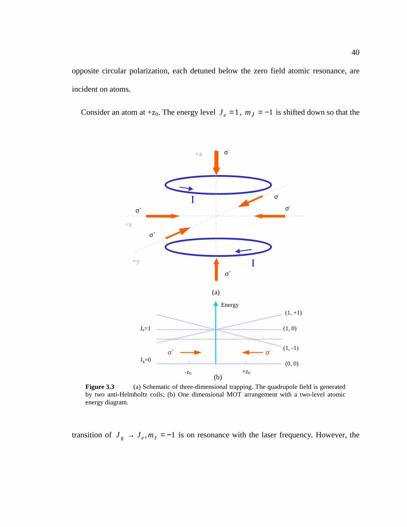
40

opposite circular polarization, each detuned below the zero field atomic resonance, are

incident on atoms.

Consider an atom at +z0. The energy level 1=eJ , 1−=Jm is shifted down so that the

transition of 1, −=→ Jeg mJJ is on resonance with the laser frequency. However, the

σ+

(a)

σ-

σ-

σ-

σ+

σ+

I

I

+x

+y

+z

(b)

(1, +1)

(1, 0)

(1, -1)

(0, 0)

Je=1

Jg=0 σ-σ+

Energy

-z0 +z0

Figure 3.3 (a) Schematic of three-dimensional trapping. The quadrupole field is generatedby two anti-Helmholtz coils; (b) One dimensional MOT arrangement with a two-level atomicenergy diagram.

41

transition of 1, +=→ Jeg mJJ is out of resonance with the laser frequency. As a result,

the atom will absorb more σ- photons than σ+ photons, and the atom is pushed toward the

origin. For an atom at -z0, the Zeeman shift is reversed, and the atom will again be pushed

toward to the origin.

Tuning the laser frequency below the atomic resonance also provides damping, as

discussed in "Optical Molasses". Therefore, confining and cooling of the atoms are

accomplished simultaneously in a MOT.

When we consider a scattering force in a MOT, the term )( υk−∆ needs to be

replaced by )('

zGkh

µυ −−∆ , where 0ωω −=∆ L , ω0 is the atomic transition without

external magnetic field and G is the magnetic field gradient. In the approximation of low

laser intensity, the total force is again given by the sum of the two radiation pressure from

each of the two beams and can be expressed as

zF καυ −−= (3.12)

where α is the same as in "optical molasses"; αµ

κk

G

h

'

= .

The size of the atomic cloud can be derived from the temperature of the MOT,

Tkz B21

21 2 =κ (3.13)

42

For a temperature of the Doppler Limit, the size of the MOT is in sub-millimeter

range.

43

4 Laser Cooling and Trapping of Metastable Krypton Atoms

4.1 Relative Krypton Atomic Transitions

Krypton gas constitutes 1 ppm (parts per million) of the earth's atmosphere in

fractional volume. It has six stable isotopes, 78Kr (isotopic abundance = 0.35%), 80Kr

(2.25%), 82Kr (11.6%), 83Kr (11.5%), 84Kr (57%), 86Kr (17.3%), and two long-lived

radioactive isotopes, 85Kr (isotopic abundance is 11102 −× ) and 81Kr (isotopic abundance

is 13105 −× ). The even isotopes have no nuclear spin. Among the odd isotopes, 83Kr and

85Kr have nuclear spin 2/9=I , 81Kr has nuclear spin 2/7=I .

A neutral krypton atom has 36 electrons. In the ground state, all shells are closed

( 610262622 43433221 pdspspss ) and the configuration is 4p6(1S0). Excited states are

formed by excitation of a valance electron from the outmost shell, which will not be

closed and therefore possesses both orbital angular momentum ( Lr

) and spin angular

momentum ( Sr

). Together with the orbital angular momentum ( lr

) and spin angular

momentum ( sr ) of the outer electron, these are coupled to form a total angular

momentum of the atom,

sKJ

ljK

SLj

rrr

rrr

rrr

+=

+=

+=

,

,

(4.1)

44

and the notation of the metastable level of the atom is [ ] JjS KnlL12 + , where n is the

outer electron's principal quantum number.

Figure 4.1 shows the atomic level diagrams of krypton. The excitation of the first

allowed transition from the ground-level 4p6(1S0) to an intermediate level 5s[3/2]1,

requires VUV photons at wavelength of 124nm. A MOT based on this transition is

impossible with present laser technology as CW lasers of this wavelength are far from

having sufficient power needed for trapping. On the other hand, Kr atoms can be excited

4p55s[3/2]2

4p55p[5/2]3

4p6

811nm

Electron Impact

4p55s[3/2]2

4p55p[5/2]2

4p6

216.7nm

216.7nm

4p55s[3/2]2

4p55p[3/2]1

4p6

4p55s[3/2]1

123.6nm

830.0nm

(a) (b)

(c)

Figure 4.1 Krypton energy level diagrams. (a) Excitation scheme used in the lasertrapping of Kr* atoms; (b) Populating the metastable level via a non-resonant UV+UVexcitation; (c) Populating the metastable level via a resonant VUV+IR excitation.

45

from the ground-level to the metastable level 5s[3/2]2 (lifetime ~ 40 s) via electron-

impact or photon excitations, and laser trapping and cooling of Kr* (metastable Kr)

atoms based on the transition 32 5p[3/2]5s[3/2] → have been realized with the laser with

wavelength of 811nm. Note that the selection rules that slow down the decay of

metastable Kr atoms break down easily upon collisions of the metastable Kr atoms with

Kr atoms (in the ground-level and in excited states), other atoms, molecules, or surface.

This characteristic makes Kr* atoms fragile and difficult to produce. On the other hand,

lack of a background of Kr* vapor makes the individual trapped atoms easier to detect.

For even isotopes, the transition 32 5p[3/2]5s[3/2] → is "closed", i.e. the excited

atoms will decay back to the lower states from where it will be re-excited by the laser

light. For odd isotopes (83Kr, 85Kr and 81Kr), metastable level 5s[3/2]2 and upper level

5p[5/2]3 split to numerous energy levels due to hyperfine interaction. The hyperfine

structure of the odd isotopes is shown in Figure 4.2. For 83Kr and 85Kr, we use the

transition 15/2F 13/2F ' =→= to cool and trap the atoms (for 81Kr,

13/2F 11/2F ' =→= ). In practice, those transitions are not perfectly "closed". It is

possible that, for 83Kr and 85Kr, the atoms will be excited to the neighboring upper states

F' =13/2 or F'=11/2 (for 81Kr, F'=11/2 or F'=9/2) and then decay back to F=11/2 or F=9/2

(for 81Kr, F=9/2 or F=7/2) so that the atoms will no longer interact with the laser light

tuned to the resonance of 15/2F 13/2F ' =→= (for 81Kr, 13/2F 11/2F ' =→= ). Those

atoms will become "dark" to the laser light.

The transition rate R can be calculated by

46

1

2

20

0411

21/1

−

Γ∆++==

II

Rτ

τ (4.2)

where the definitions of τ0, I0, I, ∆, Γ are the same as in Chapter 3 (see equation 3.3).

Using this equation, we can calculate the trapping transition rate and the optical pumping

Figure 4.2 Hyperfine s

relevant to trapping are drawn

Kr-8313/211/2

9/2

15/213/211/2

Kr-8113/29/27/2

13/211/29/2

Trapping1st2nd

Kr-8513/211/2

9/2

15/213/211/2

1st2nd

Trapping

Trapping 1st 2nd

tructures of the odd krypton isotopes. Note that only the levels

.

47

transition rates, therefore derive the leak rate (i.e. how fast the atom will leak to the dark

state). Ta

is 6 MH

103.1 7×

/11' =F

approxim

every 10

Figur

isotop

positi

-200 0 200 400 600 800 1000

1

2

3

8581

83

84

8682

80

Kryp

ton

Trap

Flu

o. (a

rb. u

nit)

Frequency Offset (MHz)

78

e 4.3 Fluorescence of trapped krypton atoms. Dark bands are the signals of stable

es measured with a low gain pin photo-diode detector. Line markers mark the frequency

ons of the two rare isotopes.

ke 83Kr as example, when the interacting laser beam intensity is 10 mW/cm2 and

z red-detuned to the trapping transition frequency, the trapping transition rate is

s/ , the transition rate to 2/13' =F is s/106.3 3× , and the transition rate to

2 is s/102.1 3× . Therefore, the atom will be pumped to 2/11=F

ately every 10-4 seconds; the atom will be pumped to 2/9=F approximately

-3 seconds.

48

To pump the atoms out of those "dark" lower states, a laser light with "sideband"

frequencies (for 83Kr and 85Kr, 13/2F 11/2F ' =→= and 11/2F 9/2F ' =→= ; for 81Kr,

11/2F 9/2F ' =→= and 9/2F 7/2F ' =→= ) is needed. The sideband is essential to trap

the odd isotopes of krypton at a high loading rate and to increase the lifetime of atoms in

the trap. Take 83Kr as an example, we applied 2% of the total laser power to the first

sideband and 0.5% of the laser power to the second sideband to reduce the time that the

atom spends in the dark states to shorter than 1 µs.

Atoms of different isotopes have different isotopic shifts due to their variations in the

Table 4.1 Krypton Isotopic shifts on 32 ]2/5[5]2/3[5 ps → transition (for odd isotopes, only transitions relative to trapping are listed)

Isotope Hyperfine Trapping/sidebands Calculation Measurement

81 2/92/7 → 2nd sideband -800 -795.9

83 2/112/9 → 2nd sideband -706 -711.8

85 2/112/9 → 2nd sideband -688 -687.2

81 2/112/9 → 1st sideband -309 -308.5

78 -217

80 -138

83 2/132/11 → 1st sideband -87 -88.9

85 2/132/11 → 1st sideband -77 -76.4

82 -64

84 0

86 66

81 2/132/11 → trapping 656 651.8

83 2/152/13 → trapping 783 786.9

85 2/152/13 → trapping 870 868.7

49

nuclear mass, volume and moments. When the laser frequency is tuned to the resonance

of the isotope of interest, only atoms of that particular isotope are trapped. Figure 4.3

shows the fluorescence signals of trapped Kr* atoms when the laser frequency is scanned

through the resonance of different krypton isotopes. The frequency positions of rare

isotopes are also marked in the figure. For both stable and radioactive krypton isotopes,

the isotopic shifts of 32 ]2/5[5]2/3[5 ps → have been calculated [50]. For rare krypton

isotopes (85Kr and 81Kr), the isotopic shifts of 32 ]2/5[5]2/3[5 ps → have been measured

[51]. For 85Kr measurement, a high-activity gas was separated from nuclear fission

products; for 81Kr measurement, a sample of 81Kr was produced in a reactor by neutron

activation on enriched 80Kr. The previous results on the isotopic shifts are listed in Table

4.1.

4.2 Laser System for Trapping Krypton Atoms

The all-diode-laser system is shown in Figure 4.4. The system supplies laser beams for

transverse cooling, slowing, and trapping of metastable krypton atoms.

In the system, there are three diode lasers and one tapered amplifier. The three diode

lasers are one SDL-5401 (serves as Master Laser) and two SDL 5422 (serve as Slave

Lasers). The tapered amplifier (TA) is Toptica TA-0810. For each of the lasers or the

tapered amplifier, its wavelength and mode are monitored by a wavemeter (Buleigh WA

20) and a spectrum analyzer (1.5 GHz free spectral range).

50

The Master Laser (SDL-5401) is an extended-cavity diode laser (ECDL) [52]

Slave Laser 2

Slave Laser 3

AOM2

EOM

Master Laser

FP

Ref. AOM1A

B

D

C Slowing light Light

Trapping Light

Transverse Cooling

Slave Laser 1

Slave Laser 2

Slave Laser 3

AOM2

EOM

Master Laser

FP

Ref. AOM1A

B

D

C Slowing light Light

Trapping Light

Transverse Cooling

Slave Laser 2

Slave Laser 3

AOM2

EOM

Master Laser

FP

Ref. AOM1A

B

D

CSlave Laser 2

Slave Laser 3

AOM2

EOM

Master Laser

FP

Ref. AOM1A

B

D

CSlave Laser 2

Slave Laser 3

AOM2

EOM

Master Laser

FP

Ref. AOM1A

B

D

CSlave Laser 2

Slave Laser 3

AOM2

EOM

Master Laser

FP

Ref. AOM1A

B

D

CSlave Laser 2

Slave Laser 3

AOM2

EOM

Slave Laser 2

Slave Laser 3

AOM2

EOM

Master Laser

FP

Ref. AOM1A

Master Laser

FP

Ref. AOM1A

B

D

C Slowing light Light

Trapping Light

Transverse Cooling

Slave Laser 1 Slave Laser 1 Slave Laser 1

Figure 4.4 Schematic of laser setup for trapping Kr* atoms.

51

employing a diffraction grating. Its output is 12 mW. The laser frequency is

electronically locked [53] onto a Fabry-Perot interferometer through current feedback

loop and piezoelectric transducer (PZT) feedback loop. The short-term linewidth is about

1 MHz.

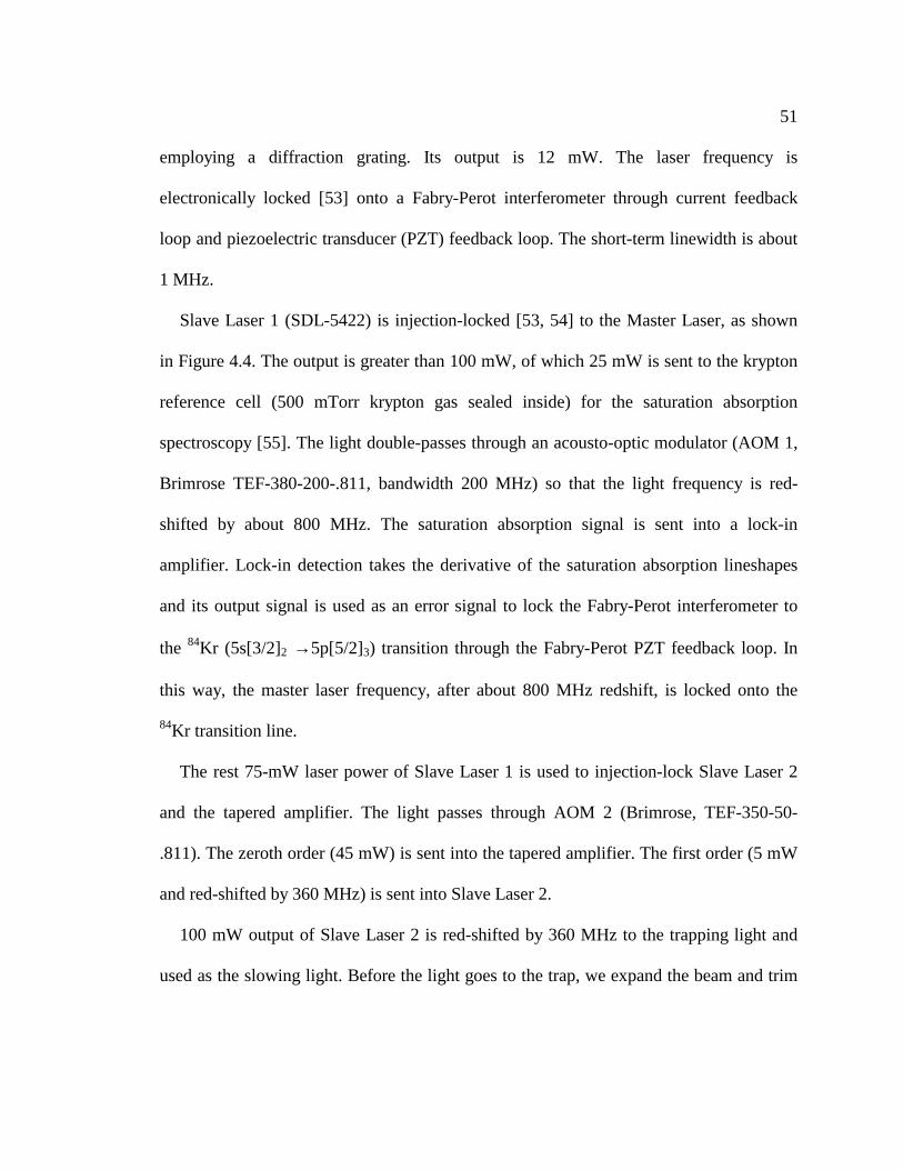
Slave Laser 1 (SDL-5422) is injection-locked [53, 54] to the Master Laser, as shown

in Figure 4.4. The output is greater than 100 mW, of which 25 mW is sent to the krypton

reference cell (500 mTorr krypton gas sealed inside) for the saturation absorption

spectroscopy [55]. The light double-passes through an acousto-optic modulator (AOM 1,

Brimrose TEF-380-200-.811, bandwidth 200 MHz) so that the light frequency is red-

shifted by about 800 MHz. The saturation absorption signal is sent into a lock-in

amplifier. Lock-in detection takes the derivative of the saturation absorption lineshapes

and its output signal is used as an error signal to lock the Fabry-Perot interferometer to

the 84Kr (5s[3/2]2 →5p[5/2]3) transition through the Fabry-Perot PZT feedback loop. In

this way, the master laser frequency, after about 800 MHz redshift, is locked onto the

84Kr transition line.

The rest 75-mW laser power of Slave Laser 1 is used to injection-lock Slave Laser 2

and the tapered amplifier. The light passes through AOM 2 (Brimrose, TEF-350-50-

.811). The zeroth order (45 mW) is sent into the tapered amplifier. The first order (5 mW

and red-shifted by 360 MHz) is sent into Slave Laser 2.

100 mW output of Slave Laser 2 is red-shifted by 360 MHz to the trapping light and

used as the slowing light. Before the light goes to the trap, we expand the beam and trim

52

the edge of the beam in order to obtain a uniform beam spatial profile. The intensity of

the slowing light is 5 mW/cm2.

The tapered amplifier has an output of 500 mW with the injection laser power of 40

mW. The fluctuation in its output is less than one percent. Long-term (10-hour) decrease

in the laser power is less than 5%. The output of the tapered amplifier is the source of

trapping light and transverse cooling light.

The two sidebands needed for repumping transitions are generated by sending the

output of the tapered amplifier through a tunable traveling-wave electro-optic modulator

(EOM, Quantum Technology, TWAP-11, up to 1.6 GHz) [56]. The modulation frequency

for 1st sideband and 2nd sideband are about 900 MHz and 1.5 GHz, respectively.

The 900-MHz frequency is generated by a voltage controlled oscillator (VCO,

MiniCircuits, ZOS-1025, up to 1 GHz). The 1.5-GHz frequency is generated by another

VCO (MiniCircuits, ZOS-1025) along with a frequency doubler (MiniCircuits, ZFL-

2500, up to 2.5 GHz) and an amplifier (MiniCircuits, ZFL-2500, up to 2.5 GHz). The two

RF signals are combined by a power combiner (MiniCircuits, ZESC-2-11, frequency

range between 10 MHz and 2000 MHz) and sent into an RF amplifier (Amplifier

Research, 5S1G4). For the frequency of 900 MHz, the input is about -2 dBm and the

output is about 34 dBm; for 1.5 GHz, the input is -5 dBm and the output is about 28

dBm.

53

The output of the amplifier is sent into the EOM, which then generates the 900-MHz

sideband with 2 percent of the total laser power and the 1.5-GHz sideband with 0.3

percent of the total laser power.

After laser beam passes through the EOM, the total laser power is 400 mW, 40 percent

of which is used for transverse cooling, the remaining 60 percent is used for trapping.

Note that the sidebands are not added to the slowing light in order to avoid the possibility

of exciting any unintended transitions inside the Zeeman slower, where the hyperfine

structure is further complicated due to Zeeman shifts.

4.3 Making of Metastable Krypton Atomic Beam

The metastable krypton atomic beam is produced by a rf-driven discharge (Figure

4.5). The discharge is driven by a rf resonator which consists of a copper coil enclosed in

a brass shield. From the upstream chamber (source chamber) to the downstream chamber

(transverse cooling chamber), krypton gas flows through a glass tube, in which a plasma

is produced by rf power coupled in from the surrounding coil. In this discharge region,

the atoms are excited from the ground state to the metastable level 5s[3/2]2 via collisions

with energetic electrons and ions.

In order to run the discharge in a good condition, several parameters have to be well

chosen. First, rf frequency is very critical for operating the discharge. Different rf

resonator may have different rf resonance frequency due to variations in coil geometry.

The resonance frequency needs to be carefully searched through the range from a few

54

tens of MHz up to a few hundred MHz. Several resonance frequencies may exist for one

resonator and line-width for each resonance frequency is approximately 10 MHz. For

instance, in our experimental setup, we can drive the discharge at 70 MHz and 230 MHz.

We found that the metastable beam flux at 230 MHz was two times that at 70 MHz when

other conditions are the same. Second, it is usually true that more rf power produces

higher metastable beam flux. But we found that higher metastable beam flux did not

always lead to higher trap loading rate. This may be due to the collisions between the

trapped atoms with more energetic ions or atoms in the trap chamber. It is also possible

that the intense discharge produces higher-temperature metastable krypton atoms, which

are difficult to be slowed down and captured. Thirdly, pressures both in upstream

chamber and downstream chamber need to be optimized. Note that a high pressure (>10

mTorr in the upstream chamber or > 4101 −× Torr in the downstream chamber) will

dramatically quench the metastable atoms. Finally, when a glass tube of the discharge is

put into the vacuum for the first time, turning on the discharge will produce a significant

amount of hydrogen and water. Flushing the glass tube with the discharge on for a certain

time period (~10 hours) before operation is necessary. How long to flush largely depends

on the humidity of location where the glass tube is stored. Usually long-time storage in a

humid environment will need extended flushing until the pressures of water and hydrogen

drop well below the operation pressure of krypton.

5

Laser spectroscopy techniques are used to measure the beam flux and the veloci

distribution (shown in Figure 4.5 (b)) [57]. The optimum metastable krypton beam flux

achieved when the pressure is about 4 mTorr in the source chamber (shown in Figure 4.6

and 5102 −× Torr in the transverse cooling chamber (shown in Figure 4.6). Under thes

conditions, we can produce a beam of metastable krypton atoms with an angular flu

density of 14104× s-1sr-1, with Kr*/Kr ratio of 10-3 and the most probable velocity of 30

m/s.

4.4 Trapping of Metastable Krypton Atoms

The krypton gas sample is injected into the vacuum system from a reservoir. In th

discharge region, a fraction of krypton atoms (about 10-3) are excited into the metastab

level. After exiting the discharge region, those atoms remain in the metastable level un

Schematic of the resonator(1) copper wire, 11 runs;(2) brass shield;(3) quartz-glass tube;(4) ceramic spacer.

Figure 4.5 (a) Schematic of RF resonator. Note that the ceramic spacer is used to isolate that end of coil from the shield. (b) Kr* beam Fluorescence vs. laser isotopes.

(a) (b)

Schematic of the resonator(1) copper wire, 11 runs;(2) brass shield;(3) quartz-glass tube;(4) ceramic spacer.

Figure 4.5 (a) Schematic of RF resonator. Note that the ceramic spacer is used to isolate that end of coil from the shield. (b) Kr* beam Fluorescence vs. laser isotopes.

Schematic of the resonator(1) copper wire, 11 runs;(2) brass shield;(3) quartz-glass tube;(4) ceramic spacer.

Schematic of the resonator(1) copper wire, 11 runs;(2) brass shield;(3) quartz-glass tube;(4) ceramic spacer.

Figure 4.5 (a) Schematic of RF resonator. Note that the ceramic spacer is used to isolate that end of coil from the shield. (b) Kr* beam Fluorescence vs. laser isotopes.

(a) (b)

5

ty

is

)

e

x

0

e

le

til

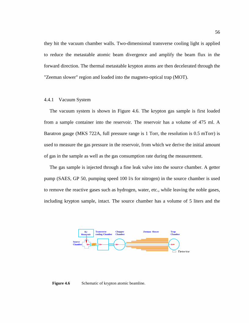
56

they hit the vacuum chamber walls. Two-dimensional transverse cooling light is applied

to reduce the metastable atomic beam divergence and amplify the beam flux in the

forward direction. The thermal metastable krypton atoms are then decelerated through the

"Zeeman slower" region and loaded into the magneto-optical trap (MOT).

4.4.1 Vacuum System

The vacuum system is shown in Figure 4.6. The krypton gas sample is first loaded

from a sample container into the reservoir. The reservoir has a volume of 475 ml. A

Baratron gauge (MKS 722A, full pressure range is 1 Torr, the resolution is 0.5 mTorr) is

used to measure the gas pressure in the reservoir, from which we derive the initial amount

of gas in the sample as well as the gas consumption rate during the measurement.

The gas sample is injected through a fine leak valve into the source chamber. A getter

pump (SAES, GP 50, pumping speed 100 l/s for nitrogen) in the source chamber is used

to remove the reactive gases such as hydrogen, water, etc., while leaving the noble gases,

including krypton sample, intact. The source chamber has a volume of 5 liters and the

Transverse cooling Chamber

Chopper Chamber

Source Chamber

Trap Chamber

Zeeman SlowerKr Reservoir

Detector

Figure 4.6 Schematic of krypton atomic beamline.

57

pressure is maintained at 4 mTorr throughout the experiment. Pressure in the source

chamber is monitored using a convectron gauge.

The source chamber and the transverse cooling chamber are connected with the glass

tube (18 cm long, 1 cm in diameter) of the rf-discharge source.

In the transverse cooling chamber, the pressure is 5102 −× Torr in the experiment.

This chamber is pumped by an oil-free, magnetically coupled turbo pump (LEYBOLD,

TurboVac 340M, pumping speed 270 l/s for nitrogen).

Between the transverse cooling chamber and the chopper chamber is a collimator (12.5

cm long, 1.6 cm in diameter) which is used to reduce the conductance between the

chambers.

Another turbo pump (LEYBOLD, TurboVac 151, pumping speed 150 l/s for nitrogen)

is used to pump the chopper chamber, which has a vacuum of 7104 −× Torr in the

Table 4.2 Vacuum system parameters.

Pressure (Torr) Pump

Source chamber 3104 −× Getter Pump

(SAES, GP 50) Transverse Cooling

Chamber

5102 −× Turbo Pump

(LEYBOLD, TurboVac)

Chopper chamber 7104 −× Turbo Pump

(LEYBOLD, TurboVac)

Trap chamber 8106 −× Turbo Pump

(Varian, V250)

58

experiment. The turbo pump is backed up by an oil-free mechanical pump (Varian,

TriScroll Dual Stage Dry Pump).

Between the chopper chamber and trap chamber is a 127-cm-long, 3.56-cm-diameter

vacuum tube. Pressure in the trap chamber is 8106 −× Torr in the experiment. The trap

chamber is pumped by a turbo pump (Varian, V-250, pump speed 200 l/s for nitrogen).

Pressures in chopper chamber and trap chamber are monitored by two ionization gauges,

respectively. The Chopper chamber also houses a residual gas analyzer for monitoring

the partial pressures of different gases in the vacuum system. The pressures and pumps in

four vacuum chambers are listed in Table 4.2.

A novel feature of the vacuum system is that it can be switched into a mode, which

repeatedly recirculates the krypton atoms through the vacuum system. This can be done

with the turbo pump in the downstream chamber pumping the krypton gas back into the

upstream chamber instead of the atmosphere, as shown in Figure 4.6. As a consequence,

this recirculation mode can dramatically increase the system efficiency for trapping and

counting the atoms.

4.4.2 Transverse Cooling

We use "two-dimensional transverse cooling" technique [58] to collimate the

metastable krypton beam. In the transverse cooling chamber, the metastable krypton

beam is cooled in both transverse directions by two sets of laser beams, each of which

has a beam size of 1 cm × 2 cm and an intensity of 40 mW/cm2. The laser beam is

59

multiply reflected between two flat mirrors (each size is 10 cm ×2 cm) and interacts with

the metastable krypton atoms over 10 cm along the atomic beam flux once the atoms exit

the discharge region. For each dimension, one of the two mirrors is mounted outside the

chamber and is adjustable, the other is fixed inside the chamber.

With one-dimensional transverse cooling, we can enhance the trap loading rate by

factor of 8. With two-dimensional transverse cooling, an enhancement factor of 20 to 25

can be achieved. Note that this process is isotopically selective; it only enhance the

forward atomic beam flux and therefore the trap loading rate of the selected isotope. Also

note that, when the laser frequency is tuned to the transition of odd isotopes of krypton,

the sidebands in the transverse cooling light can optical pump the atoms in the states of

2/11=F and 2/9=F into 2/13=F state for 83Kr and 85Kr (optical pump the atoms in

the states of 2/9=F and 2/7=F into 2/11=F state for 81Kr).

4.4.3 Slowing Down the Atoms with Zeeman Slower

We use the "Zeeman Slowing" technique to longitudinally slow down the atomic

beam. The required slowing magnetic field (see Equation 3.5) is produced by a tapered

solenoid, which is wound with wires in many layers of different lengths (shown in Figure

4.7). Each layer is a uniform solenoid, which produces a magnetic field B_solenoid along

the axis of the solenoid

−+

−−

−+

−=

22

22

21

210

)()(2)(_

zZr

zZ

zZr

zZnIzsolenoidB

µ (4.3)

60

where n is "turns per cm"; I is current; Z1 is the position of one end of the solenoid; Z2 is

the position of the other end of the solenoid. The magnetic field produced by the tapered

solenoid is the sum of the magnetic fields produced by each layer uniform solenoid. The

parameters of the tapered solenoid, such as lengths of the layers and the current, need to

be well designed in order to produce a smoothly varying magnetic field that can meet the

requirement of slowing down the atoms.

Downstream from the chopper chamber, the metastable krypton atoms enter 50-inch-

long Zeeman slower, where they are decelerated by a circular-polarized laser beam from

a velocity of approximately 300 m/s near the source to 20 m/s as they enter the trap

chamber. The laser beam (with a frequency of 360 MHz red-detuned to that of the

trapping light) has an intensity of 5 mW/cm2 in the trap chamber and is gently focused

(a)

B-fie

ld

Z (a lo n g th e a to m ic b e a m lin e )

(b)

(a)

B-fie

ld

Z (a lo n g th e a to m ic b e a m lin e )

(b) Figure 4.7 (a) Schematic of a Zeeman slower; (b) Slowing magnetic field profile.

61

from the trap chamber up to the discharge region. This schematic is applied to reduce the

atomic beam divergence when the atoms are slowed down in the Zeeman slower.

4.4.4 Magneto-Optical Trap (MOT)

On the trap chamber, a pair of anti-Helmholtz coils (MOT coils) are wound to provide

the quadrupole field required by the MOT, which has a field gradient of about 3

Gauss/cm along the horizontal axis (Figure 3.3). The equations on the magnetic field

produced by the pair of coils are as follows. Along the z-axis (Figure 3.3), the magnetic

field Bz(z) is

-20 -10 0 10 20

-20

-15

-10

-5

0

5

10

15

20

B-fie

ld (G

auss

)

distance from the central point (cm) along Z-axis (blue); along horizontal axis (red)

Figure 4.8 MOT field profile along the horizontal axis and vertical axis. In thiscalculation, coil radius 35.6=r cm; distance between the two coils 985.6=d cm;current 450×=I Amp.

62

])2

([])2

()[2(4

)( 5.1225.12220 −− −−+−−+= zbrzbrIrzBz ππ

µ (4.4)

where 1.040 ×= πµ ; r is radius of the coils; I is the current flowing through the coils; b

is the distance between the two coils. Along the horizontal axis of MOT, the magnetic

field Bx(x) is

θθ

θπ

µ π dxrdxr

rdxBx ∫−++

= 20

5.12

22

0

)]sin(24

[

)sin(4

)( (4.5)

Near the central point of the MOT, the gradient of magnetic field along the z-axis is

about two times the gradient of magnetic field along the horizontal axis. A MOT

magnetic field profile is shown in Figure 4.8.

The "End" coil, wound at the end of the atomic beamline, is used to compensate the

residue magnetic field of the slowing solenoid at the center of the chamber. By tuning the

current of the End coil, we can fine-tune position of the trap in the direction along the

atomic beam. The "Horizontal-Trim" coils and "Vertical-Trim" coils are installed to fine-

tune the position of the trap in the horizontal direction and in the vertical direction,

perpendicular to the atomic beam.

Each of three pairs of trapping laser beams has an intensity of 10 mW/cm2 and a beam

size of 3 cm in diameter. The frequency of trapping light is 6 MHz red-detuned to the

atomic transition.

4.4.5 Detection of Trapped Atoms

63

Since the trapping light is infrared, the trap can not bee seen by naked eyes. We use

the Charged Coupled Device (CCD) camera to detect the fluorescence of the trapped

atoms and the fluorescence image can be monitored on a monitor. With the CCD camera,

we can qualitatively study the shape and the brightness of the trap.

To measure the number of the trapped atoms, we use a PIN Photo-diode (detection

area is 20.4 mm2, quantum efficiency is approximately 0.8 at 811nm) with a gain of 108

Ω. The detector is put in front of one viewport of the trap chamber and is 13 cm away

from the trap. The geometric photon-collection efficiency is about 10-4, i.e. every 1 out

10,000 photons emitted from the trapped atoms is collected by the PIN detector.

The number of trapped atoms reaches a maximum when the loading rate of atoms is

equal to the loss rate of the atoms in the trap. Equation (4.2) describes the evolution of

the number of trapped atoms during the loading period,

2NNLdtdN β

τ−−= (4.6)

where L is loading rate; the first loss term τ/N is due to the collisions between the

trapped atoms and the thermal background atoms, τ is about 0.5 seconds when the

pressure in the trap chamber is maintained at 8106 −× Torr; the second loss term 2Nβ is

due to the collisions between pairs of trapped atoms. Generally speaking, when the

loading rate is high ( 810≥ atoms/second), loss is dominated by the second loss term and

the loading time (defined as the time taken to load 63% (1-1/e) of atoms under

equilibrium into the trap) is short (~20 ms); when the loading rate is low, especially in the

64

condition of single atom detection (discussed in Chapter 5), the first loss term dominates

and the lifetime of the single atom in the trap is about 0.5 seconds.

Therefore when we calculate a high trap loading rate using (4.2), we can drop the first

loss term and only keep the second loss term. The solution is

1

1)(2

2

+

−=tL

tL

e

eLtNβ

β

β (4.7)

The trap loading rate can be derived as follows. When the trap reaches the equilibrium,

βLtN =∞→ )( (4.8)

This number of trapped atoms can be measured with the PIN detector. Then we measure

the time difference ∆t between when the trap reach 10% of the equilibrium trapped atom

number and when the trap reach 50% of the equilibrium trapped atom number. Using

(4.3), it is easy to get

tL

∆= 11

27ln2 β (4.9)

Combining (4.4) and (4.5), we have

ttNL∆

∞→= )(9.0 (4.10)

Under the optimum condition, a 83Kr trap loading rate of 9103× atoms per second can

be achieved with a trap loading time of 20 ms.

65

In the condition of single atom detection, the second loss term can be neglected in the

calculation. Solving the equation (4.2), we have

)1()( /0

τteNtN −−= (4.11)

where τLN =0 . The loading time is equal to τ.

66

5 Single Atom Detection

The isotopic abundances (I.A.) of 85Kr and 81Kr are approximately 11102 −× and

13106 −× [4, 9, 59], respectively. With the loading rate of 83Kr (I.A.=11.5%) at 9103×

atoms/s, we expect the loading rate for 85Kr and 81Kr to be between 10-3/s and 10-1/s.

Since the lifetime of the trapped atoms is 0.5 seconds at a pressure of 8106 −× Torr in the

trap chamber, the rare krypton atoms do not accumulate in the trap; instead they are

usually captured one at a time. Therefore, the system must be able to detect a single atom

in the trap.

In single atom detection, the main technical challenge is to reduce the background

photons scattered off walls, windows, and even the optics outside the vacuum chamber. It

takes at least 10 mW of light to maintain the trap, while only 2 pW of light is emitted by

a trapped krypton atom.

5.1 Spatial Filter

The schematic of the optical system for single atom detection is shown in Figure 5.1.

Each of the four identical lenses has a diameter of 25 mm and a focal length of 50 mm.

The lens closest to the trap is located inside the trap chamber and is 50 mm away from

the trap. The other three lenses are installed along a tube. The single atom emits

approximately 107 photons per second, of which one percent are collected and imaged by

one pair of the lenses, through an aperture (diameter is tunable, minimum is 0.6 mm)

67

which spatially filters out most of the diffuse background light, and re-imaged by another

pair of lenses onto the detector. An electronic shutter (Melles Griot, 04 IES 211) is

installed in front

In order to re

trap chamber is

Technology, ML

Torr). In order t

of the nearby

deliberately mis

5.2 Avalanch

Figure 5.1

the viewport o

box.

Aperture Shutter

Trap Detector

Schematic layout of the optical system for single atom detection. Dashed line is

f the trap chamber; dotted line is the tube; dashed and dotted line is the electronics

of the detector and used to prevent the detector from over-exposure.

duce the scattering light from the chamber walls, the inner surface of the

coated with a vacuum-compatible black paint. The paint material (AZ

S-85SB) is specially designed for high vacuum systems (down to 10-11

o reduce the scattering light from the optics outside the trap chamber, all

mirrors and quarter-waveplates are carefully aligned, and sometimes

-aligned.

e Photon Detector (APD) and Electronics

68

We use an APD (EG\&G SPCM-AQ-21) as the single atom detector. The APD has a

dark count of 860 counts/s and a pulse_width of 30 ns. The quantum efficiency at 811nm

is 25% and the detection active area is 0.5 mm in diameter. The APD has a gating

function: when the voltage in the gate input is TTL-high (5 V), the detector is enabled;

when the voltage is TTL-low, the detector is disabled. Based on this function, a

protection circuit is used to prevent the APD from damage due to over-exposure. The

maximum count rate of the APD is 13 MHz.

The APD is housed in an electronic box, whose inner walls are also covered with the

black paint to reduce the scattering background. Inside the box, the APD is installed on a

three-axis translation stage (Newport, 423 series) which can be used to fine-adjust the

position of the APD. The resolution of the translation stage in each axis is 1 µm.

R1

R2

CAPD BNC

TTL:30 ns, 5 volt TTL:1 us, 5 volt

To PC

VPulse Train Pulse Train

R1

R2

CAPD BNCR1

R2

C

R1

R2

CAPD BNC

TTL:30 ns, 5 volt TTL:1 us, 5 volt

To PC

VPulse Train Pulse Train

Figure 5.2 Electronics for single atom detection.

69

Figure 5.2 shows the electronics for single atom detection, which can convert photon

count rate into a voltage output. The APD detects a train of photons and converts it into a

train of electronic TTL pulses (30 ns, 5 Volt). A pulse generator (Berkeley Nucleon

Corporation, Model 8010) expands the TTL pulses from 30 ns to 1 µs (pulse_width is

adjustable). An integrator circuit then integrates the train of the pulses in time and

converts the pulse signals into a voltage signal V at its output,

( ) ( )VoltPsV RR 51

12 ⋅⋅⋅−= µ (5.1)

where R1 and R2 are the input and feedback resistors in the integral circuit; 1 µs and 5

Volt are the pulse_width and the amplitude of the TTL signal at the input of the integral

circuit; and P is the photon counting rate. In our integrator circuit, R1=15 kΩ, R2=33 kΩ,

the capacitor C=0.33 µF; the integration time is 10 ms. For a 20 kHz photon counting

rate, the voltage signal is about 200 mV.

5.3 Single Atom Signal

Before we could count individual 85Kr and 81Kr atoms, we optimize the conditions of

single atom detection by obtaining clear 83Kr single atom signals.

The optimal conditions for single atom detection are quite different from the optimal

trap loading conditions. To achieve a high loading rate, we use large (3 cm in diameter)

and strong (10 mW/cm2) trapping laser beams and a moderate magnetic field gradient of

the MOT (8 Gauss/cm). However, when detecting, in order to reduce the scattering light,

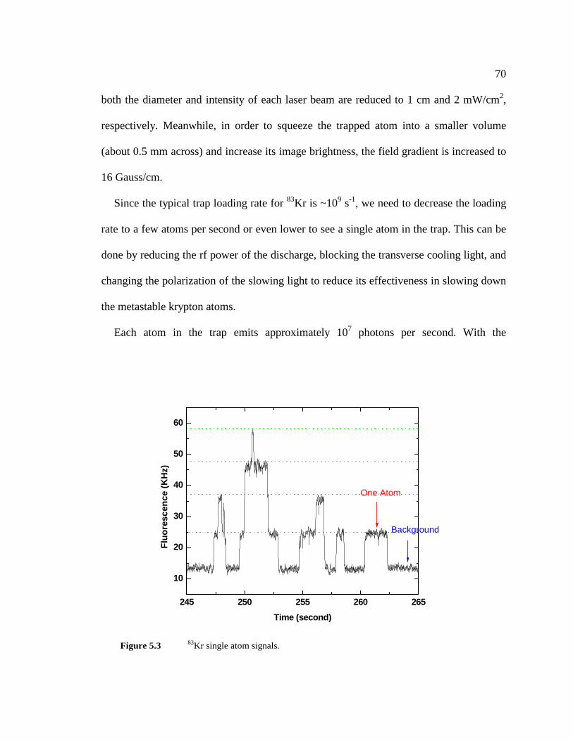
70

both the diameter and intensity of each laser beam are reduced to 1 cm and 2 mW/cm2,

respectively. Meanwhile, in order to squeeze the trapped atom into a smaller volume

(about 0.5 mm across) and increase its image brightness, the field gradient is increased to

16 Gauss/cm.

Since the typical trap loading rate for 83Kr is ~109 s-1, we need to decrease the loading

rate to a few atoms per second or even lower to see a single atom in the trap. This can be

done by reducing the rf power of the discharge, blocking the transverse cooling light, and

changing the polarization of the slowing light to reduce its effectiveness in slowing down

the metastable krypton atoms.

Each atom in the trap emits approximately 107 photons per second. With the

245 250 255 260 265

10

20

30

40

50

60

One Atom

Background

Fluo

resc

ence

(KH

z)

Time (second)

Figure 5.3 83Kr single atom signals.

71

combination of geometric efficiency (1%) and the quantum efficiency of the APD (25%),

the ideal single atom signal is about 25 kHz. Figure 5.3 shows the 83Kr single atom

signals we recorded. The single atom signal is 13 kHz and the background is 13 kHz. The

signal to noise ratio of 15 with 10 ms integration time is achieved. In the figure, one, two,

three, and four atoms in the trap can be clearly identified.

72

6 Counting Individual 85Kr and 81Kr Atoms

Since the isotopic abundance of rare krypton atoms is very low, we need to run the

system at the maximum trap loading rate. Meanwhile, we also need to detect single atoms

in the trap. However, as we discussed in the last chapter, the trap loading conditions are

significantly different from the single atom detection conditions. In order to meet these

two sets of requirements, switching between "capture mode" (trap loading) and "detection

mode" (single atom detection) is needed when we detect 85Kr and 81Kr in the trap.

6.1 Switching Between Capture Mode and Detection Mode

The optimal conditions for trap loading and single atom detection are listed in Table

6.1,

Table 6.1 The optimal conditions for trap loading and single atom detection.

Capture Mode Detection Mode

Diameter of trapping

beams 3 cm 1 cm

Intensity of trapping

beams 10 mW/cm2 2 mW/cm2

MOT field gradient 8 Gauss/cm 16 Gauss/cm

Atomic beam On Off

APD detector Off On

73

A schematic diagram of trapping light switching is shown in Figure 6.1. The switching

Large

Small

(1) (2)

Large and strong

Small and weak beam

Shutter 1

Shutter 2

Vertical trapping beam

Horizontal trapping beam 1

Horizontal trapping beam 2

Large and strong Beam

Small and weak beam

Shutter

Shutter 2

Vertical trapping beam

Horizontal trapping beam 1

Horizontal trapping beam 2

(1) Large beam is ON; small beam is OFF

(2) Large beam is OFF; small beam is ON

Figure 6.1 Schematic of trapping light switching.

74

is accomplished with two electronic shutters (Vincent Associates, LS3T2), each of which

has a rise time of less than 1 ms and is controlled by a Uniblitz 212 shutter controller.

The controller is triggered by an external TTL input, which determines the shutter

exposure and closure time. In the figure, Beamsplitter 1 distributes 40% of the large beam

into the vertical trapping light, the other 60% goes to the horizontal trapping light.

Beamsplitter 2 is 50/50. In the capture mode, the large beam (vertical - 16 mW/ cm2, each

horizontal - 12 mW/ cm2) is on while the small beam is off; in the detection mode, the

small beam (vertical - 6 mW/ cm2, each horizontal - 2 mW/ cm2) is on while the large

beam is off.

Switching of magnetic field gradients is accomplished with a high-current switching

V+

+-

+-

+12 V

Power

10 KΩΩΩΩ10 KΩΩΩΩ

10 KΩΩΩΩ10 KΩΩΩΩ

220 PF

0.1 ΩΩΩΩ

MOT coil

MOSFEET

V-

Figure 6.2 Schematic of high-current switching system. 1.01−=

VI , +− = VV .

75

system. The schematic is shown in Figure 6.2. The MOT coil current I is controlled by an

external TTL input with a MOSFET (BUK 453-60A).

When the input is TTL-high (5 Volt), V- is high and as a result the current is large (13

A in the experiment); when the input is TTL-low (zero), V- is low and the current is small

(5 A in the experiment). In this system, a diode is used to relieve the current when

switching is from large current to small current. Since the large current runs through the

MOSFET and 0.1 Ω resistor, the electronics board becomes hot in a long run and

therefore a heat sink or a fan is needed. The 0.1 Ω resistor (OHMITE 850-RE75G series)

has a high stability (±90 ppm/degree), which is important in order to keep the two current

conditions highly stable. In our one-day experimental run, the large current and small

current are both stable within 0.005 Ampere. The response time of the current switching

is 4 ms.

An electronic shutter is installed in front of the APD detector to protect the detector

from overexposure. In the capture mode, the shutter is closed; in the detection mode, the

shutter is open.

When switching from capture mode to detection mode, the atomic beam is turned off

in order to eliminate the scattering light off the atomic beam in the trap chamber. This is

realized with an "Atomic Chopper", whose schematic is shown in Figure 6.3. This

mechanical chopper consists of an in-vacuum stepper motor (MDC, SM23-HV, vacuum

range 8105 −× Torr) and a U-shape blade symmetrically mounted on the top of the

stepper motor axis. When the stepper motor is in operation, the blade will be rotating

76

along the axis. The atomic chopper is installed inside the chopper chamber and can

periodically block the metastable krypton beam, essentially turning on and off the beam

going into the trap chamber.

Figure 6.3 also shows that the slowing light will be chopped while the atomic beam is

being chopped. A photodetector is installed in front of the viewport on the source

chamber to receive the chopped slowing light signal, which is then shaped into a TTL

signal. The TTL signal, as a trigger input, is sent to a pulse generator (BNC, Model

500A), which has four output channels to control switching of the laser beams, MOT coil

current switching, and switching (on and off) of electronic shutter in front of the APD.

With this schematic, all the switching is synchronized to the position of the atomic

chopper.

Atomic Chopper

Slowing Light Atomic Beam

Stepper

Detector

U-Blade rotating

Figure 6.3 Schematic of "atomic chopper", which is a mechanic chopper consisting of astepper motor and a U-shape blade mounted on the tip of the stepper motor.

77

The timing diagram of TTL signal at the input and the four synchronized outputs is

shown in Figure 6.4. The rotating period of atomic chopper is determined by the stepper

motor speed, which is adjustable. In our experiment, the period is 385 ms. The duty cycle

of the trigger input is determined by the shape of the U-shape blade. In the experiment,

the atomic beam ``ON'' time is 285 ms, "OFF" time is 100 ms.

For each channel output of BNC, the pulse_width and delay to the trigger input can be

285 ms

100 ms

270 ms

105 ms

265 ms

115 ms

270 ms

105 ms

290 ms

60 ms

Atomic Beam

Large Laser Beam

Small Laser Beam

MOT Coil Current

APD detector

ON

OFF

ON

OFF

ON

OFF

Large

Small

ON

OFF

(1) (2)

(1) (2)

(1) (2)

(1) (2)

Figure 6.4 Timing diagram of BNC input and outputs. The "useful" period is (1)+(2).

78

set independently. Note that the "useful" period (from the rising edge of the trigger input

to the time when the channel output is back to its initial state) of each channel is set to be

a few milliseconds shorter than the period of the trigger input. If the "useful" period is

longer than the trigger period, the channel will not be triggered by the rising or falling

edge of the next TTL pulse until it finishes its current period, which will result in the

channel idling for the next period.

Another note is that the large trapping laser beam and small trapping laser beam

cannot be off at the same time during switching, or the trapped atoms will escape due to

the interruption of trapping laser beams. In order to avoid that, we set up 5 ms

overlapping time between large beam and small beam.

Moreover, in order to keep the strong scattering background due to the large laser

40 41 42 43 440

5

10

15

20

25

30

35

One Atom

Background

Phot

on C

ount

ing

Rat

e (K

Hz)

Time (second)

Figure 6.5 85Kr single atom signal. Time constant of the circuit is about 10 ms and thesignal to noise ratio is 15 within 10-ms integration time.

79

beams or the atomic beam fluorescence from falling into the detector exposure time

period, 60 ms "ON" time for APD is set much shorter than any other detection time

parameters.

6.2 85Kr and 81Kr Single Atom Signal

85Kr single atom signals are shown in Figure 6.5. The signals are the output of the

integral circuit (in Chapter 5) and the time constant of the circuit is about 10 ms. The

single atom signal is about 13 KHz and the background is 15 KHz. In the loading period,

the APD detector is blocked and about 2 KHz background is mainly due to the dark

current.

6.3 Computerized Data Acquisition

Single atom signals at the output of integral circuit can be monitored and recorded by

both oscilloscope and computer. But since signals at the output of the integral circuit are

analog, the size of data acquired and recorded by computer is very large and therefore

requires a significant fraction of CPU time to process and a large amount of memory to

store.

80

To solve the pro

Figure 6.6

a 30-minute tim

Signal to noise

790 795 8000

200

400

600

800

1000

1200

1400

1600

1800

2000

2200

2400

Phot

on C

ount

ing

(in 6

0 m

s)

Time (second)

0 200 400 600 800 1000 1200 1400 1600 18000

200

400

600

800

1000

1200

1400

1600

1800

2000

2200

2400

Phot

on C

ount

s (in

60

ms)

Time (second)

(a)

(b) 81Kr single atom signal with new schematic of data acquisition. Upper graph is

e train of atom counting of 81Kr; lower graph is a zoom-in picture in 10 seconds.

ratio is greater than 45.

blem, a new schematic of data acquisition was implemented including

81

a PC and National Instruments' LabView instrumentation. A LabView interface board is

configured to read two digital inputs. One input (Gate) is gate signal that is the same as

the signal sent to the electronic shutter in front of APD (details in chapter 5). The other

input (Atom Count) is the TTL signal directly from the output of the pulse generator

(Chapter 5). For each period of atom counting, the PC counts the number of TTL pulses

when "Gate" is TTL-high; it stops counting when "Gate" is TTL-low. Single atom

counting of 81Kr is shown in Figure 6.6. The signal is the TTL pulse number (also the

photon number) counted by PC in 60 ms. The upper graph is 30-minute time train of

atom counting of 81Kr. The lower graph is a Zoom-in picture in 10 seconds. With this

schematic, the signal to noise in integration time of 60 ms is greater than 45.

82

7 85Kr and 81Kr Abundance Measurement

In 81Kr-dating, age is defined as the time since water or ice sample was near the

surface and had contact with the atmosphere. Once the water went underground and ice

froze, they were separated from the atmosphere, and the 81Kr abundance started to

decrease according to

τ/0)( teNtN −= (7.1)

where τ is the lifetime of 81Kr, N0 is the atmospheric isotopic abundance of 81Kr, N(t)

is the isotopic abundance of 81Kr in the sample, and t is the age of the sample.

7.1 Control Isotope and Ratio Measurements

The isotopic abundance of 81Kr can be determined by the ratio of the trap loading rates

of 81Kr and a control isotope with known isotopic abundance. The trap loading rate of an

individual isotope depends on the isotopic abundance and many parameters of the

apparatus including the discharge intensity, gas flow rate, various vacuum pressures,

partial pressure of krypton, laser beam intensity, laser frequencies, laser beam alignment,

etc. Our system is stable after about half an hour of warm-up. The loading rate for 83Kr

typically drifts less than 15% in a 10-hour run. By frequently switching the system

between counting 81Kr and counting the control isotope, much of the common mode

noise due to the variation of all the parameters is cancelled out in the ratio. Furthermore,

the age is determined by the ratio of the isotopic abundance of 81Kr in the sample and in

83

the atmosphere; in fact it is a measurement of a ratio of ratios, which further reduces the

systematic effects.

In principle, the stable 83Kr can be used as the control isotope. But in practice, its trap

loading rate ~109 atoms/s is so much higher than that of 81Kr that, instead of single atom

detection, it requires a different detector system such as a low gain pin photo-diode

detector to measure the fluorescence of the trapped 83Kr atoms. Meanwhile, due to the

collisions between pairs of trapped atoms, the trap lifetime of 83Kr (20 ms) is much

shorter than that of a single trapped 81Kr atom (~0.5 second). These differences make

83Kr a less reliable control isotope. On the other hand, 85Kr with the isotopic abundance

of ~10-11, can be introduced into the sample and calibrated accurately with the LLC

method. The "spiked" 85Kr can then be counted at the single atom level and serve as a

reliable control isotope. The age of the sample can be calculated as

( )( )

=

sss

aaaNNNN

t858581

858581////

lnρρτ (7.2)

where N81s and N81a are counting rates of 81Kr atoms from the sample and from air,

respectively; N85s and N85a are counting rates of 85Kr atoms from the sample and air,

respectively; ρ85s and ρ85a are LLC calibration of 85Kr isotopic abundance from the

sample and air, respectively. The spike and LLC of 85Kr involve mature technologies that

are practiced on a routine basis in a few selected labs around the world.

7.2 Laser Frequency Mapping

84

Laser frequency setting affects the trap loading rates; it affects the abundance

768 770 772 774 776 778 780 782 784 7860

20

40

60

80

100

120

140 Trap Freq. - 777 MHzTrans. Freq. - 783 MHz

Kr83

Loa

ding

Rat

e (a

rbi.

units

)

Frequency (MHz)

854 856 858 860 862 864 866 868 870 8720

10

20

30

40

50

60 Trap Freq. - 864 MHzTrans. Freq. - 870 MHz

Kr8

5 C

ount

s (e

ach

poin

t in

10 m

in.)

Frequency (MHz)

638 640 642 644 646 648 650 652 654 6560

5

10

15

20

25

30

35Trap Freq. - 647 MhzTrans. Freq. - 653 MHz

Kr8

1 Co

unts

(eac

h po

int i

n 2

hour

s)

Frequency (MHz)

Figure 7.1 Frequency Mapping. (a) 83Kr loading rate vs. trapping frequency; (b) 85Kr

loading rate vs. trapping frequency, a 10-minute measurement is taken for each data point; (c)81Kr loading rate vs. trapping frequency, a 2-hour measurement is taken for each data point.

85

measurement, which is done by measuring ratio of trap loading rates of two different

isotopes; but it should not affect the age, which is derived from the isotopic abundances

of two samples ideally analyzed under identical laser frequency settings. Therefore, the

repeatability of laser frequency setting from one run to another is crucial to age

determination. A drift in laser frequencies can lead to a systematic error in age. The

significance of this effect can be studied by mapping out the laser frequency dependence

of trap loading rate of 83Kr, 85Kr and 81Kr. Furthermore, in order to count the atoms at the

maximum trap loading rate, we need to find out the optimum laser frequency settings.

From Figure 7.1(a), we conclude that the optimum trapping frequency for 83Kr is 6

MHz red-shifted from its transition frequency. For 85Kr (Figure 7.1(b)), the maximum

loading rate is about 45 atoms in 10 minutes. The optimum trapping frequency is about

864 MHz blue-shifted to the 84Kr transition [ ] [ ] 32 2/552/35 ps → . If we assume that the

optimum trapping frequency for 85Kr is also 6 MHz red-tuned to its transition, we can

derive that its transition frequency is 870 MHz blue-shifted to the 84Kr transition. For

81Kr (Figure 7.1(c)), the maximum loading rate is about 14 atoms in an hour. The

optimum trapping frequency is 647 MHz blue-shifted to the 84Kr transition. Its transition

frequency is 653 MHz blue-shifted to the 84Kr transition if we use the same assumption

as for 85Kr. Our transition frequency results are in good agreement with that measured by

Cannon [51]. The laser frequency, locked to the [ ] [ ] 32 2/552/35 ps → transition of 84Kr

in the vapor cell, has a repeatability of better than 0.5 MHz, which should cause the trap

loading rate to shift by less than 4%.

86

We have also mapped out loading rate vs. 1st sideband and loading rate vs. 2nd

sideband for both 83Kr and 85Kr. The results (listed in Table 7.1) are also in good

agreement with Cannon's work. For either isotope, the loading rate drops by factor of 2

when either 1st sideband frequency is tuned 20 MHz away from its optimum frequency

or the 2nd sideband is 40 MHz away from the optimum frequency. This broad frequency

dependence is due to power broadening; the rates of repumping transition provided by the

laser intensity of the sidebands far exceed the needed repumping transition rates. We

Table 7.1 Frequency Comparison between Cannon's work and this work.

Cannon's work This work

83Kr - transition 786.9 MHz 783 MHz

83Kr - 1st sideband -88.9 MHz -87 MHz

83Kr - 2nd sideband -711.8 MHz -707 MHz

85Kr - transition 868.7 MHz 870 MHz

85Kr - 1st sideband -76.4 MHz -78 MHz

85Kr - 2nd sideband -687.2 MHz -676 MHz

81Kr - transition 651.8 MHz 653 MHz

81Kr - 1st sideband -308.5 MHz

81Kr - 2nd sideband -795.9 MHz

87

conclude that the effect on trap loading rates due to any changes of sidebands is

negligible.

7.3 Switching Between Different Isotopes

From measuring one isotope to the other, there are only three parameters to switch:

isotope shift which is controlled by the AOM frequency and the two sideband frequencies

which are controlled by the EOM frequencies. These switches are performed either

manually or automatically with computer control.

88

8 An Atom Trap System For Practical 81Kr-dating

As we discussed in chapter 2, due to its extremely low isotopic abundance, there are

only roughly 1,000 81Kr atoms in one liter of groundwater. Moreover, due to the low

concentration of krypton in the atmosphere, only approximately 60 µl STP of krypton can

be extracted from 1,000 liters of groundwater. For practical 81Kr-dating of groundwater,

20,000 liters of groundwater may be the upper limit for practical Earth Sciences studies.

That amount of groundwater provides approximately 400 µl STP of krypton gas sample,

in which there are only 7102× 81Kr atoms. A 10% measurement of that krypton gas

sample requires the analysis system to achieve system efficiency larger than 5101 −× .

Meanwhile, the system also needs to operate with krypton samples as small as a few

hundred µl STP.

8.1 Gas Handling System

Figure 8.1 shows the schematic of gas handling system, which is designed to operate

with small gas samples (~100 µl STP).

The sample is contained in a metal cell with a NuPro valve, which can be attached to

one end of the reservoir, as shown in Figure 8.1. The reservoir has a volume of 475 ml

and when 100 µl STP of krypton gas sample is released into the reservoir, the pressure in

the reservoir rises to about 150 mTorr. The maximum amount of sample gas that can be

measured with the Baratron gauge in the reservoir is approximately 500 µl STP. The gas

89

sample is injected from the reservoir into the source chamber through a fine leak valve

(Granville-Phillips, 216 Servo Driven Valve Assembly), which is operated by a flow

controller (Granville-Phillips, Model 216). A fill of 30 µl STP of krypton gas into the

vacuum syst

for rf discha

The reser

routinely us

connected to

be pumped

vacuum syst

8.2 Gas R

Figure 8.

samples (

from Kr bottle

to system

Reservoir

Sample Cell

to roughing pump

from Ar(or N2) bottle

Needle Valve

1 Schematic of a gas handling system developed to handle small krypton gas

~100 µl STP).

em will increase the source chamber pressure to 4 mTorr, which is optimal

rge operation.

voir is also connected to a bottle of commercial krypton gas, which is

ed to check and to optimize the system. The argon (or nitrogen) gas bottle

the reservoir is used to flush the system (discussed later). The reservoir can

by a roughing pump through a long pipe or by a turbo pump through the

em.

ecirculation

90

When the vacuum system is operated in recirculation mode, the krypton gas sample is

repeatedly recirculated through the vacuum system and therefore the system counting

efficiency can be dramatically improved. A schematic of gas recirculation is shown in

Figure 8.2.

In each stage of gas recirculation, a turbo pump pumps the krypton gas through a

vacuum tube from the downstream chamber back to the upstream chamber (stage 1: from

transverse cooling chamber to source chamber; stage 2: from chopper chamber to

transverse cooling chamber; stage 3: from trap chamber to transverse cooling chamber).

Stage #1: source chamber - 4 mTorr; transverse cooling chamber - 2 × 10-5 Torr; Turbo pump - 270 l/s; tube conductance 12 l/s. recirculation tube - 12 inch long, 3/2 inch in diameter. Stage #2: chopper chamber - 4 × 10-7 Torr; Turbo Pump - 150 l/s; tube conductance 0.9 l/s. recirculation tube - 24 inch long, 3/4 inch in diameter. Stage #3: trap chamber - 6 × 10-8 Torr; Turbo Pump - 200 l/s; tube conductance 0.3 l/s. recirculation tube - 84 inch long, 3/4 inch in diameter.

Stage #1

Stage #2

1 2 3 4

Stage #3

From Reservoir

Figure 8.2 Schematic of gas recirculation.

91

The vacuum tubes need to be properly chosen in order to minimize the amount of

krypton gas stored in the recirculation loops. There are two factors to be considered: one

is the volume of the recirculation loop, the other is the pressure in the loop. On one hand,

using thin tubes will reduce the volume of the loop, thereby decrease the amount of

krypton gas accumulated in the loop. But on the other hand, thin tubes have small

conductance, which will make a large amount of gas accumulate in the back of turbo

pump, where the pressure is much higher than the chambers. The conductance of the

vacuum tube should be compatible with the pumping speed of the turbo pump and can be

calculated by

RL

AC

831

41

+=

υ (8.1)

where C is conductance; υ is velocity of the thermal atoms (300 m/s for krypton atoms

at room temperature); A is the cross sectional area of the tube; L is length of the tube; R

is radius of the tube.

In our system, the tube conductance C1 in the first stage is about 12 l/s; in the second

stage, C2 is about 0.9 l/s; in the third stage, C3 is 0.3 l/s. To operate the whole vacuum

system with the optimal pressures, we need to fill 30 µl STP of krypton gas into the

system. And we estimate that there is approximately 10% of krypton gas in the

recirculation loops.

92

Without the gas recirculation, the total counting efficiency is about 7101 −× . With the

first stage of recirculation, the system efficiency is increased to about 6108 −× ; with the

first two stages of recirculation, the efficiency is about 5104 −× ; and with all three stages

of recirculation, we achieve an system efficiency of 4102 −× in 7 hours for 30 µl STP of

krypton sample.

Ideally the krypton sample can be recirculated indefinitely in the system, however the

run time is limited for two reasons: cross-sample contamination (discussed later) and

argon outgassing.

When the system is in recirculation mode, the getter pump is the only pump for the

system. As we discussed in chapter 4, it can pump nitrogen at the speed of 100 l/s. It can

also efficiently remove other reactive gases, such as water and CO2, while leaving the

noble gases including krypton intact. Argon is an abundant noble gas and will accumulate

due to outgassing in the vacuum system. We use a RGA (Residual Gas Analyzer) to

monitor the pressures of different gases in the vacuum system. Over 10 hours, the partial

pressure of argon in the chopper chamber can increase from below 910− Torr up to

7101 −× Torr, or 50% of the krypton pressure. As a result, the krypton metastable beam

flux is reduced and so is the trap loading rate. This effect requires the system to be

pumped out after 10 hours of recirculation. The loss of krypton sample during the

pumping-out limits the average times of recirculation to ~3000, and the counting

efficiency of the system to 4103 −× .

93

8.3 Cross-sample Contamination

When the rf-discharge is on, a small fraction of krypton atoms are ionized, accelerated

by the rf field, and imbedded into the surface of the glass tube. Meanwhile, the previously

embedded krypton atoms are released into the vacuum by the discharge. We observe an

initial reduction of 3 µl STP of krypton, or 10% of the sample in one fill, within the first

two hours after the discharge is turned on, and a total reduction of 6 µl STP, or 20% of

one fill, in 8 hours. The loss rate gradually decreases to zero as the krypton atoms in the

vacuum reach equilibrium with the embedded krypton atoms. We maintain a constant

krypton pressure by refilling a few percent of krypton gas periodically throughout the

experiment.

Obviously the embedded krypton atoms would be a serious source of cross-

0 500 1000 1500 2000 25001E-9

1E-8

1E-7

1E-6

Flushing with Argon RF-Discharge

Argon

Krypton

Pres

sure

(Tor

r)

Time (second)

Figure 8.3 Cross-sample contamination

94

contamination. This is confirmed in the following test. After one measurement, the

system is pumped out and filled with argon. The krypton pressure dramatically increases

when the argon discharge is turned on, as shown in Figure 8.3. The amount of krypton

released is measured to be 3 µl STP in half an hour.

We solve the contamination problem by flushing the glass tube with the discharge of

Figure 8.4 F

flushing, the krypto

0 10000 20000 30000 40000 50000

1E-9

1E-8

1E-7

1E-6

1E-5

1E-4

Pres

sure

(Tor

r)

Time (second)

Nitrogen

Krypton

@ Nitrogen discharge on

0 5000 10000 15000 20000 25000 30000

1E-9

1E-8

1E-7

1E-6

Pres

sure

(Tor

r)

Time (second)

Krypton

Argon

@ Argon discharge is on after 13 hour flushing with N2 discharge

(a)

(b) lushing with the discharge of nitrogen. (a) flushing for 13 hours; (b) after

n pressure increase up to 8103.1 −× Torr, which is about 7% contamination.

95

nitrogen or argon. We use nitrogen as the "cleaner" because nitrogen can be removed by

the getter pump. The result is shown in Figure 8.4. We first flush the glass tube with

nitrogen discharge for more than 13 hours. Then we turn on the argon discharge to see

the krypton contamination after the flushing. In eight hours, the krypton pressure

increases up to 8103.1 −× Torr, which is about 7% contamination. Note that the average

contamination in a run is 50% of the final contamination level.

The effect of contamination on the 81Kr/85Kr ratio measurement can be expressed as

follows,

ε)( 0'' rrrr −+= (8.2)

where r is the actual ratio of the krypton sample; r' is the measured ratio of the krypton

sample; r0 is ratio of the krypton contaminant (depending on the history of

measurements); ε is the contamination level. Furthermore the ratio of modern krypton

81Kr/85Kr ratio to sample 81Kr/85Kr ratio can be derived as

εε )1(1

1)(

'

0'

0

0''

00

−−=

−+=

rrr

rrrr

rr

r (8.3)

The effect of contamination on age determination can then be expressed as follows,

−−=

ετ

)1(11ln '

'

RRt (8.4)

96

where t is the age of the sample; τ is the lifetime of 81Kr; '

0'

rrR = ; ε is the contamination

percentage.

97

9 ATTA vs. LLC -- Double-Blind Test

Our system has achieved a system efficiency of 4102 −× and is capable of operating

with the krypton gas sample as small as 30 µl STP. In order to demonstrate the capability

of our system on quantitative measurements, we measured the 85Kr/81Kr ratios of a group

of krypton gas samples prepared by Purschert et al. at the University of Bern,

Switzerland. All of these samples are derived from young air samples (less than 80 years

old) and therefore the isotopic abundances of 81Kr are expected to be identical. On the

other hand, the abundances of 85Kr were prepared to be different and were measured with

LLC at University of Bern. Note that, for each sample, we did not know the 85Kr

abundance measured with LLC until we finished our ratio measurement and sent our

result to Bern for comparison. Therefore, the test is indeed "double-blinded".

9.1 Procedures

Each time before we start to analyze a new sample, we flush the system with nitrogen

discharge for at least 10 hours in order to reduce the cross contamination below

approximately 3%.

In an analysis, the system is filled with approximately 30 µl STP of krypton sample

and run for typically 6 hours. An analysis run consists of many (averagely 8) cycles, with

each cycle taking 40 minutes: 30 minutes for counting 81Kr followed by 10 minutes for

counting 85Kr.

98

After 6 hours, argon will accumulate due to its outgasssing so that the partial pressure

in the chopper chamber increases up to approximately 8106 −× , or 30% of the krypton

pressure. We then pump out and refill the system for another analysis run.

For each sample, we perform several analysis runs that mainly depend on the sample

size and precision requirement.

9.2 Results and Data Analysis

We measured the first three test samples (O1, O2, O3) from 09/28/02 - 10/02/02. We

analyzed one sample (ANL) from a bottle of commercial krypton gas and four more test

samples (F1, F2, F3, F4) in February 2003. We analyzed the last test sample (M1) from

University of Bern in March 2003. The results are shown in Table 9.1.

Column 2 lists the sample size of each krypton gas sample. Column 3 lists the sample

volume we actually used. Generally speaking, 100 µl STP of krypton gas is a favorable

size for our system, but we can also operate with as small as 30 µl STP of krypton

sample. Column 4 lists the total number of analysis cycles for each sample. Column 5 is

the number of 81Kr atoms being counted for each sample. Column 6 is the number of 85Kr

atoms being counted for each sample. Column 7 is the 85Kr/81Kr ratio of each sample.

The error is determined using the formula

2

81

812

85

852

+

=

CC

CC

RR δδδ (9.1)

99

where R is the 85Kr/81Kr ratio and 8185 /3 CCR = , δR is the error of the ratio; C85 is the

Table 9.1 Rusults of test sample measurements.

Sample Volume (µl STP)

Used

Volume(µl STP)

# of

runs

# of 81Kr

# of 85Kr

Ratio of 85Kr/81Kr

LLC (dpm)

O1 167 113 28 166 231 4.17±0.42 14.4±1.6

O2 63(1) 40 16 94 525 16.8±1.9 85±5

O3 122 65 26 165 213 3.87±0.40 14.4±1.6

ANL (2) (3) 24 121 659 16.3±1.6 59±3.2

F1 86 75 15 61 405 19.9±2.7 64.9±5

F3 198 56 22 113 255 6.77±0.77 27.7±1.1

F2

(PreBomb)(4) >600 (5) 17 79 17 0.65±0.17 (6)

F4 118 71 30 127 802 18.9±1.8 74.2±4

M1 442 61 20 84 365 13.0±1.6 45±3

M2 (spiked

PreBomb)(7) 296 171 48 158 1254 23.8±2.0 81.2±5

This sample is not pure krypton gas, but a mixture of 40 µl STP of krypton and 23 µl STP of air.

(1) Sample "ANL" is from a bottle of commercial krypton gas.

(2) We did not measure the sample volume we consumed.

(3) The PreBomb sample was extracted from the the atmosphere by a German company before

1945 (between 1933 and 1940).

(4) Since the sample size is larger than 500 µl STP, the Baratron gauge cannot read the pressure in

the reservoir and therefore we could not measure the sample volume we consumed.

(5) LLC of this sample shows the decay rate of 85Kr is less than 0.8 dpm. (6) This sample is also made from the same reservoir as "F2"..

100

number of 85Kr counts, δC85 is the statistical error of C85 ( 8585 CC =δ ); C81 is the

number of 85Kr counts, δC81 is the statistical error of C81 ( 8181 CC =δ ). Column 8 is the

results of 85Kr abundance measured with LLC at University of Bern.

85Kr/81Kr ratios measured with ATTA vs. 85Kr/Kr ratios measured with LLC is plotted

out in Figure 9.1. A fitting line is also shown in the figure.

There are a few things to be mentioned. First, Sample "O1" and "O3" are from the

same krypton reservoir and the ratio measurements by ATTA are indeed consistent with

each other. Therefore we can combine those two measurements to produce a more precise

result 29.002.4 ± . Secondly, Sample "O2" is not a pure krypton gas, but a mixture of

krypton gas and air due to a vacuum leak in the sample preparation system, which is both

0 20 40 60 80 100

0

5

10

15

20

25

ATTA

(Kr8

5/Kr

81)

LLC (dpm)

Y=a*X+ba=0.238+-0.012b=0.643+-0.163Reduced chi-squared 1.32

Figure 9.1 A comparison between ATTA and LLC. In ATTA, the 85Kr/81Kr ratios are measured. In LLC, the decay of 85Kr are counted, and the unit is dpm/cc (decay per minute percc STP of krypton).

101

measured by RGA in our vacuum system and confirmed by Bern group. Moreover, "O2"

is not from the same krypton sample as the one measured by LLC, although the two

krypton samples were collected by the Bern group on the same day. Therefore it is

possible that the two samples had different 85Kr abundances. We remove this point in the

following data analysis. Thirdly, Sample "F2" is from a krypton reservoir that was

collected by a German company between 1933 and 1940, therefore it is a pre-nuclear

sample. The importance of this sample is that not only it serves as one data point in the

test, but also it indicates the level of cross-contamination by measuring the ratio of

85Kr/81Kr since no 85Kr is expected to be detectable in the pre-nuclear krypton gas. We

did count 85Kr atoms in this sample at the 85Kr/81Kr ratio level of 17.065.0 ± , or the level

of 4% cross-contamination if we assume the contaminant is modern krypton. Our former

cross-contamination measurement using RGA is approximately 2~3%. Therefore we

assigned the cross-contamination level to be %2%4 ± . The calibration of cross-

contamination is expressed as follows (see also chapter 8),

ε)( 0'' rrrr −+= (9.2)

where r is actual 85Kr/81Kr ratio of the sample; r' is measured 85Kr/81Kr ratio of the

sample; r0 is the modern krypton 85Kr/81Kr ratio; ε is the cross-contamination level (here

again we assume the contaminant is modern krypton).

After (1) combining "O1" and "O3"; (2) excluding "O2"; (3) correcting the

systematical error due to the cross-contamination for each data point, the data points and

the fitting curve are plotted out in Figure 9.2. Several conclusions can be drawn from the

102

figure. First, the linear correlation between 85Kr/81Kr ratios measured by ATTA and 85Kr

abundance measured by LLC demonstrated the validity of ATTA analysis. Secondly, the

81Kr abundance can be derived from the slope of linear correlation if we assume that the

system efficiencies for 85Kr and 81Kr are identical. The value is 1310)8.06.12( −×± ,

which disagrees with the previous measurements (with LLC or AMS) by at least 5

standard deviations, as shown in Figure 9.3.

9.3 81Kr Abundance of Pre-Nuclear Krypton Sample

81Kr abundances in the pre-nuclear krypton and post-nuclear krypton were expected to

be identical, which were predicted by a detailed analysis of possible sources (see chapter

1) and confirmed by measurements with AMS. After we finished our double-blind test

with LLC, we also did the measurement to compare the 81Kr abundance of pre-nuclear

0 10 20 30 40 50 60 70 80 90 100

0

5

10

15

20

25

ATTA

(Kr8

5/Kr

81)

LLC (dpm)

Y=a*X+ba=0.265+-0.017b=-0.100+-0.324reduced Chi-squared 0.53

Figure 9.2 A comparison between ATTA and LLC after calibration of the cross-contamination effect (see the context).

103

krypton gas and of post-nuclear krypton gas. A ~300 µl STP of pre-nuclear krypton

sample was supplied by the Bern group. The sample was made from the same krypton

reservoir as Sample "F2" and spiked with 85Kr. Like the double blind test, the Bern group

did LLC m

(results are

85Kr/81Kr r

consistent

shown in F

Figure

perform

0

2

4

6

8

10

12

14

Kr-

81/K

r (X

10-1

3 ) LLC1969

LLC1983

AMS1997

ATTA1999

ATTA 2003 -- (12.6+-0.8)X10-13

Prebomb - (11.3+-1.2)X10-13

ATTA2003

Prebomb

9.3 Comparison between ATTA result of 81Kr/Kr and other measurements

ed by LLC and AMS.

easurement of 85Kr/Kr ratio and we did ATTA measurement of 85Kr/81Kr ratio

listed in Table 1). The LLC result is 52.81 ± dpm/cc. ATTA result of

atio is 0.28.23 ± . The derived 81Kr abundance is 1310)2.13.11( −×± , which is

with 81Kr abundance of modern krypton within one standard deviations (as

igure 9.3).

104

10 ATTA 81Kr-dating of the Ancient Groundwater of Nubian Aquifer in Western Egypt

With the success of double-blind test with LLC, we are in the position to apply our

method on the real-world problems. The first application is to date the groundwater

samples of Nubian Aquifer in Western Egypt. As we discussed in the previous chapters,

81Kr-dating of these ancient groundwater samples will determine the residence time of the

Nubian Aquifer, which could address a number of problems relating to the origin and

history of the Nubian Aquifer. On the technical side, this work will further demonstrate

the capability of our method in practical 81Kr-dating and lead to other applications in

environmental research.

10.1 Nubian Aquifer

Nubian Aquifer, one of the world's largest groundwater reservoirs, lies beneath the

surface of the hyperarid Western Desert of Egypt, adjacent portions of eastern Libya,

northeastern Chad and northwestern Sudan (shown in Figure 10.1). The area of the

aquifer is approximately 6102× km2 and the volume of the aquifer is approximately

4105× km3, which is equivalent to 500 years of Nile River discharge.

The Nubian aquifer has two major basins: the Kufra Basin of Libya, northeastern

Chad, and northwestern Sudan and the Dakhla Basin of Egypt. The aquifer reaches a

depth of 3,000 m in the center of the Dakhla Basin. Groundwater of the Dakhla Basin

area flows from southwest to northeast and discharge naturally at oases. The recharge of

105

the aquifer is minor compared with the discharge. Two models were proposed to explain

the origin of the groundwaters: (1) large-scale flow from mountainous recharge areas in

the southwest [60]; (2) recharge during previous more humid climatic conditions that

prevailed throughout the present desert area [61].

On the basis of the existing 14C data and 36Cl data, it is believed that a significant

fraction of the groundwater in the Nubian Aquifer may have a residence time longer than

400,000 years. The 36Cl data cannot supply reliable age information mainly due to the

uncertainties of 36Cl/Cl data caused by the subsurface production of 36Cl. The 81Kr/Kr

data, however, have the potential to resolve these fundamental issues and help understand

the history of the aquifer.

10.2 Groundwater Sampling

The Nubian Aquifer groundwater sampling trip led by Neil Sturchio, a geologist at the

University of Illinois at Chicago, was carried out in May, 2002.

Six groundwater samples for trace analysis of 81Kr were collected at six wells in the

Western Desert of Egypt, respectively (Figure 10.2). The sampling sites are: Kharga,

Baris, El Zayat, Dakhla, Farafra and Bahariya (shown in Figure 10.1). Gases were

extracted from 5 - 10 tons of water samples on site by spraying the water into the

evacuated chamber and compressing the gas into gas cylinders (shown in Figure 10.3).

The gas samples (each has a volume of approximately 300 liters STP) were shipped to

the University of Bern for krypton separation and purification.

106

To complement the 81Kr analyses and place them in a broader geochemical and

isotopic context, a set of other chemical and isotopic analyses of the water samples has

been and is being performed. Temperature and pH values of the water were recorded at

each sampling site. The interpretation of all these data is out of the scope of this thesis

and will be covered in a later publication.

10.3

Figu

The

re 10.1 Location map showing the Nubian Aquifer. 5 oases are indicated in the map.

El Zayat oasis (not shown in the figure) locates between Dakhla and Kharga, near Dakhla.

Krypton Sample Preparation

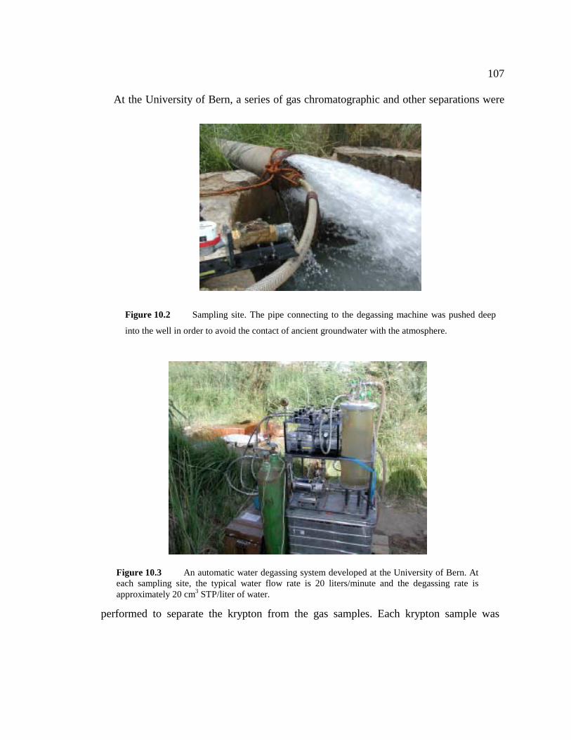
107

At the University of Bern, a series of gas chromatographic and other separations were

performed to separate the krypton from the gas samples. Each krypton sample was

Figure 10.2 Sampling site. The pipe connecting to the degassing machine was pushed deep

into the well in order to avoid the contact of ancient groundwater with the atmosphere.

Figure 10.3 An automatic water degassing system developed at the University of Bern. Ateach sampling site, the typical water flow rate is 20 liters/minute and the degassing rate isapproximately 20 cm3 STP/liter of water.

108

spiked with 85Kr that serves as control isotope. For each sample, 85Kr isotopic abundance

was measured by LLC measurement. The spiked krypton samples (each has a volume of

~100 µl STP) were sealed in a steel container with a NuPro valve and sent to Argonne

National Laboratory for 81Kr analysis.

10.4 81Kr-dating: Procedures and Results

The procedures are the same as in the double-blind test (see Chapter 9).

So far, we have analyzed two of seven samples. The results are shown in Table 10.1.

We were informed by the group at University of Bern that the krypton sample were

mixed with less than 10% of methane (CH4). We did find that amount of methane, which

had a negligible effect on the experiment. Meanwhile, we found a significant amount of

helium in the sample (He/Kr ratio ~ 1:1). High helium pressure quenched the metastable

krypton atoms and reduced the trap loading rate of krypton atoms. Now this problem has

been solved by pumping the helium out of the sample container through the reservoir and

Table 10.1 Experimental results of two water samples.

Sample Volume (µl STP)

Used

Volume (µl STP)

# of

runs

# of 81Kr

# of 85Kr

Ratio of 85Kr/81Kr

LLC (dpm)

Farafra 82 40 15 5 181 109±49 80.5±8.1

Baris 500 120 34 29 773 80±15 80.5±8.1

109

the vacuum system while keeping the krypton in the sample container with liquid

nitrogen cooling. This can be realized because the boiling point of krypton (120 0K) is

higher than nitrogen (77 0K) while helium (4.55 0K) is lower.

The Farafra sample size is 82 µl STP (including helium). We actually used

approximately 40 µl STP of krypton. The sample was measured in 15 cycles. 5 counts of

81Kr and 181 counts of 85Kr were accumulated. Ratio of 85Kr/81Kr is 109±49.

For Baris sample, we used approximately 120 µl STP of krypton. In three

experimental runs (34 cycles), 29 counts of 81Kr and 773 counts of 85Kr are accumulated.

The ratio of 85Kr/81Kr is 80±15.

10.5 Data Aanlysis

Using Equation (8.4), we can derive the age information from the ratio of 81Kr/85Kr

ratio (or 81Kr isotopic abundance) in modern krypton to 81Kr/85Kr ratio (or 81Kr isotopic

abundance) in the water samples.

81Kr isotopic abundance in modern krypton is 1310)8.06.12( −×± (see Chapter 9).

81Kr isotopic abundance in water sample is derived from our measurement of 81Kr/85Kr

ratio and LLC measurement of spiked 85Kr isotopic abundance in the samples.

Cross-sample contamination level is 4% ± 2% (see Chapter 9).

The age information of the two samples is listed in Table 10.2.

110

The results of the first two water samples setup a new milestone for ATTA - Radio-

Krypton dating of ancient groundwater for the first time.

A comparison with 36Cl data as well as sample measurements is necessary. It is

beyond the scope of this thesis to give a hydrological interpretation of the results.

However the preliminary 81Kr result showed that the Baris sample is surprisingly old.

With the success of the first 81Kr-dating of the ancient groundwater, we are very

confident that more measurements of these two samples and other water samples will

supply reliable age information on the groundwater in the Nubian Aquifer.

Table 10.2 Two water sample age information.

Water Sample 81Kr isotopic abundance

(10-13) Age (kyr)

Farafra 2.48±1.15 596±195

Baris 3.37±0.72 474±89

111

Reference

1. J. Arnold and W. Libby. Age determination by radiocarbon content: checks with

samples of known age. Science 110, 678 (1949).

2. W. Libby. Radiocarbon dating. Nobel Lecture, December 12, 1960.

3. W. Kutschera. Accelerator mass spectrometry: a versatile tool for research. Nucl.

Instr. Meth. B 50, 252 (1990).

4. P. Damon et al. Radiocarbon dating of the Shroud of Turin. Nature 337, 611

(1989).

5. Isotopes of noble gases as tracers in environmental studies. (Vienna, Austria,

1989)

6. Edited by P. Cook and A. Herczeg. Environmental tracers in subsurface

hydrology. (2000)

7. Edited by L. Currie. Nuclear and chemical dating techniques. (1982)

8. Edited by W. Alley. Regional ground-water quality. (1993)

9. J. Ahearne. Radioactive waste: the size of the problem. Physics Today Vol. 50,

No. 6, 24 (1997); K. Crowley. Nuclear waste disposal: the technical challenges. Physics

Today Vol. 50, No. 6, 32 (1997).

10. M. Apted et al. Yucca mountain: Should we delay?. Science 296, 2333 (2002).

11. H. Oeschger. Accelerator mass spectrometry and ice core research. Nucl. Instr.

Meth. B 29, 196 (1987).

112

12. J. Petit et al. Climate and atmospheric history of the past 420,000 years from the

Vostok ice core, Antarctica. Nature 399, 429 (1999).

13. D. Schoen. Learning from polar ice core research. Environmental Science and

Technology Vol. 33, Issue 7, 160A (1999).

14. R. Alley and M. Bender. Greenland ice cores: frozen in time. Sci. Am. 266, 80

(February, 1998).

15. A. Wilson and D. Donahue. AMS carbon-14 dating of ice: progress an future

prospects. Nucl. Instr. Meth. B 52, 473 (1990).

16. W. Broecher. Chaotic climate. Sci. Am. 263, 62 (November, 1995).

17. W. Kutschera. Accelerator mass Spectrometry: analyzing our world atom by

atom. AIP conference 495, 407 (1999).

18. W. Kutschera et al. Long-lived noble gas radionuclides. Nucl. Instr. Meth. B 92,

241 (1994).

19. F. Hippel, D. Albright and B. Levi. Stopping the production of fissile material for

weapons. Sci. Am. 253, 40 (1985).

20. H. Loosli. A dating method with 39Ar. Earth Planet. Sci. Lett. 63, 51 (1983).

21. W. Broecker and T. Peng. Comparison of 39Ar and 14C ages for waters in the deep

ocean. Nucl. Instr. Meth. B 172, 473 (2000).

22. B. Lehmann. Counting radioactive noble gas atoms: lasers, accelerators or decay

counters? Resonance Ionization Spectroscopy 2000, edited by J. Parks and J. Young

(AIP, New York, 2001).

113

23. Edited by A. Jull et al. Methods of low-level counting and spectrometry. (IAEA,

Vienna, 1981).

24. H. Loosli et al. Ten years low-level counting in the underground laboratory in

Bern, Switzerland. Nucl. Instr. Meth. B 17, 402 (1986).

25. H. Loosli and H. Oeschger. 37Ar and 81Kr in the atmosphere. Earth Planet. Sci.

Lett. 7, 67 (1969).

26. Proceedings of the 8th International Conference on Accelerator Mass

Spectrometry. Nucl. Instr. Meth. B 172 (2001).

27. R. Muller. Radioisotope dating with a cyclotron. Science 196, 489 (1977).

28. D. Elmore and F. Phillips. Accelerator mass spectrometry for measurement of

long-lived radioisotopes. Science 236, 543 (1987).

29. W. Kutschera. Accelerator mass spectrometry: a versatile tool for research. Nucl.

Instr. Meth. B 50, 252 (1990).

30. P. Collon et al. Measurement of 81Kr in the atmosphere. Nucl. Instr. Meth. B 123,

122 (1997).

31. P. Collon et al. 81Kr in the Great Artsian Basin, Australia: a new method for

dating very old groundwater. Earth Planet. Sci. Lett. 182, 103 (2000).

32. P. Collon. A new method to detect cosmogenic 81Kr. Ph.D. Thesis (University of

Vienna, Austria 1999).

114

33. I. Ahmad et al. Ultra-high-sensitivity measurements and investigation of

fundamental interactions. Physics Division Annual Report 2001, Argonne National

Laboratory.

34. Private Communication with P. Collon.

35. G. Hurst et al. Method for counting noble gas atoms with isotopic selectivity.

Rep. Prog. Phys. 48, 1333 (1985).

36. B. Lehmann et al. An isotope separator for small noble gas samples. Nucl. Instr.

Meth. B 28, 571 (1987).

37. N. Thonnard and R. Willis, M. Wright and W. Davis. Resonance Ionization

Spectroscopy and the detection of 81Kr. Nucl. Instr. Meth. B 29, 398 (1987).

38. B. Lehmann, H. Loosli, D. Rauber, N. Thonnard and R. Willis. 81Kr and 85Kr in

groundwater, Milk River aquifer, Alberta, Canada. Appl. Geochem. 6, 419 (1991).

39. W. Fairbank Jr. Photon burst mass spectrometry. Nucl. Instr. Meth. B 29, 407

(1987).

40. W. Fairbank Jr. Photon burst mass spectrometry for the measurement of 85Kr at

ambient levels. SPIE 3270, 174 (1998).

41. C.-Y. Chen, Y. Li, K. Bailey, T. O'Connor, L. Young and Z.-T. Zheng.

Ultrasensitive isotope trace analysis with a magneto-optical trap. Science 286, 1139

(1999).

115

42. Z.-T. Lu, K. Bailey, C.-Y. Chen, X. Du, Y. Li, T. O'Connor and L. Young. Atom

trap trace analysis. Atomic Physics 17, edited by E. Arimondo, P. Denatale, and M.

Inguscio (AIP 2001).

43. H. Metcalf and P. Straten. Laser cooling and trapping. (1999).

44. Edited by S. Chu and C. Wieman. Laser cooling and trapping of atoms. J. Opt.

Soc. Am. B Vol. 6, No. 11 (1989).

45. W. Phillips. Laser cooling and trapping of neutral atoms. In Laser Manipulation

of Atoms and Ions, edited by E. Arimondo, W. Philipps, and F. Strumia, Proceedings of

the International School of Physics "Enrico Fermi".

46. W. Phillips, J. Prodan and H. Metcalf. Laser cooling and electromagnetic trapping

of neutral atoms. J. Opt. Soc. Am. B Vol. 2, 1751 (1985).

47. W. Ertmer, R. Blatt, J. Hall and M. Zhu. Laser manipulation of atomic beam

velocities: demonstration of stopped atoms and velocity reversal. Phys. Rev. Lett. 54, 996

(1985).

48. W. Phillips and H. Metcalf. Laser deceleration of an atomic beam. Phys. Rev.

Lett. 48, 596 (1982)

49. E. Raab, M. Prentiss, A. Cable, S. Chu and D. Pritchard. Trapping of neutral

sodium atoms with radiation pressure. Phys. Rev. Lett. 59, 2631 (1987).

50. A. I. Ludin and B. E. Lehmann. High-resolution diode-laser spectroscopy on a

fast beam of metastable atoms for detecting very rare krypton isotopes. Appl. Phys. B 61,

461 (1995).

116

51. B. D. Cannon. Hyperfine spectra of the radioactive isotopes 81Kr and 85Kr. Phys.

Rev. A 47, 1148 (1993)

52. A. S. Arnold, J. S. Wilson and M. G. Boshier. A simple extended-cavity diode

laser. Rev. Sci. Instr. 69, 1236 (1998).

53. C. E. Wieman and L. Hollberg. Using diode lasers for atomic physics. Rev. Sci.

Instr. 62, 1 (1991)

54. H. R. Telle. Injection locking of a 1.3 µm laser diode to an LiNdP4O12 laser yields

narrow linewidth emission. Electron. Lett. 22, 150 (1986)

55. A. Corney. Atomic and Laser Spectroscopy (1977)

56. J. F. Kelly and A. Gallagher. Efficient electro-optic modulator for optical

pumping of Na beams. Rev. Sci. Instr. 58, 563 (1987)

57. C.-Y. Chen et al. Beam of metastable krypton atoms extracted from a rf-driven

discharge. Rev. Sci. Instr. 72, 271 (2001)

58. W. Rooijakkers, W. Hogervorst and W. Vassen. An intense collimated beam of

metastable helium atoms by two-dimensional laser cooling. Opt. Commun. 123, 321

(1996)

59. V. V. Kuzminov and A. A. Pomanski. Radiocarbon 22, 311 (1980)

60. J. Ball. Geographical Journal 70, 21 (1927)

61. U. Thorweihe. Hydrogeologie des Dakhla Berkens (Agypten). Berliner Geowiss.

Abh. A38, 1 (1982)