Realization of preconditioned Lanczos and conjugate gradientalgorithms on optical linear algebra processors

Anjan Ghosh

Lanczos and conjugate gradient algorithms are important in computational linear algebra. In this paper, aparallel pipelined realization of these algorithms on a ring of optical linear algebra processors is described.The flow of data is designed to minimize the idle times of the optical multiprocessor and the redundancy ofcomputations. The effects of optical round-off errors on the solutions obtained by the optical Lanczos andconjugate gradient algorithms are analyzed, and it is shown that optical preconditioning can improve theaccuracy of these algorithms substantially. Algorithms for optical preconditioning and results of numericalexperiments on solving linear systems of equations arising from partial differential equations are discussed.Since the Lanczos algorithm is used mostly with sparse matrices, a folded storage scheme to represent sparsematrices on spatial light modulators is also described.

I. Introduction

Hybrid optoelectronic processors capable of ma-nipulating matrices and vectors are known as opticallinear algebra processors (OLAPs). Parallel imple-mentations of several algorithms of computational lin-ear algebra (such as, Gaussian elimination, QR decom-position, Richardson and Jacobi iterations) on OLAPshave been described in the last few years.1

In this paper, we describe a parallel pipelined real-ization of the preconditioned conjugate gradient (CG)and Lanczos algorithms2 on a ring of OLAPs. For thesolution of a linear system of equations, the CG algo-rithm is just a special case of the iterative Lanczosalgorithm. The reasons for considering a parallel opti-cal realization of these algorithms are given below:

(1) The CG is a popular algorithm in computationallinear algebra and is used extensively in the solution oflarge systems of linear algebraic equations arising inthe numerical solutions of partial differential equa-tions.2

(2) Being a nonlinear second-order algorithm, theCG and Lanczos algorithms converge to the globalsolution faster than most of the linear first-order itera-tive algorithms do.

The author is with University of Iowa, Department of Electrical &Computer Engineering, Iowa City, Iowa 52242.

Received 15 December 1987.0003-6935/88/153142-07$02.00/0.© 1988 Optical Society of America.

(3) The CG algorithm has uses in spectral estima-tion3 and may be helpful in adaptive signal processing;the Lanczos algorithm can be used for computing QRor singular value decompositions, 2 most essential inparallel signal processing.

(4) If preconditioning operation is performed,Lanczos and CG algorithms become robust and canwithstand high values of round-off errors, especiallythose in the analog OLAPs.4

Thus an optoelectronic implementation of Lanczosand CG algorithms helps in efficiently solving a widevariety of engineering problems ranging from finite-element-based structural analysis to signal processing.The robustness of these algorithms makes them suit-able for analog OLAPs; we can properly utilize the highparallelism and fast throughput rates5 in spite of thenoise and errors present in these processors.

Optoelectronic implementations of the standard CGalgorithm have been considered previously in Refs. 6-8, but the most important issue of the numerical accu-racy of an optical realization is analyzed for the firsttime in this paper. We have observed that the spatialerrors and detector noise in the OLAPs reduce theaccuracy of the final solution and decrease the rate ofconvergence of the standard CG algorithm significant-ly. Thus for optical implementation of the CG algo-rithm one must introduce the preconditioning and usethe more general and powerful Lanczos algorithm. Aparallel systolic implementation of the Lanczos algo-rithm on OLAPs is proposed and analyzed in thispaper, we believe for the first time.

These algorithms have an intricate structure. Ineach iteration several matrix-vector and vector-vectorinner products are necessary along with many scalar-

3142 APPLIED OPTICS / Vol. 27, No. 15 / 1 August 1988

vector operations. We execute the time-consumingoperations of vector multiplications in parallel to ob-tain the maximum throughput. The flow of data fromone processor to another and the feedback of databetween iterations are the most important factors de-termining the speed and efficiency of a ring of proces-sors. We design the data flow to minimize idle times ofthe processors and the redundancy of computations.

Usually, the operations of matrix preconditioningare embedded in the CG iterations as an inner loop.2

We find that such an inner loop increases idle time.Therefore, we perform matrix preconditioning as aseparate operation in which the matrix data are pro-cessed first and then passed onto the main ring ofOLAPs executing the CG and Lanczos iterations.9 Wedevised a simple but OLAP-realizable algorithm formatrix preconditioning. An optical preprocessor withthis preconditioning algorithm can be efficiently cou-pled to the main OLAP to improve the accuracy of theoverall computation. We conducted several numeri-cal experiments to quantize the effects of optical errorson the convergence and accuracy of the multiprocessorrealizing the preconditioned Lanczos algorithm.

The CG algorithm is often used with large sparsematrices, and for an optoelectronic realization of thisalgorithm to be viable, optical handling and storage ofsparse matrices should be considered. Thus in thispaper we describe a folded storage scheme to representsparse matrices on spatial light modulators.

In Sec. II we describe the Lanczos and conjugategradient algorithms. A pipelined realization of theLanczos algorithm on a ring of OLAPs is described inSec. III. A parallel algorithm for matrix precondition-'ing and its optical realization are discussed in Sec. IV.The results of numerical experiments carried out toquantize the effects of optical errors are described inSec. V. In Sec. VI we discuss the important issue ofsparse matrix processing on optical processors. InSec. VII we offer our conclusions.

II. Lanczos and Conjugate Gradient Algorithms

Lanczos algorithm is a versatile algorithm used inevaluating eigenvalues and eigenvectors and solvingleast-squares problems. It can be used for iterativelysolving a system of linear algebraic equations

Ax = b, (1)

where A is an (N X N) coefficient matrix, b is a knownN vector, and x is the unknown N vector. The CGalgorithm is a special case of the iterative Lanczosalgorithm.

The Lanczos algorithm can be stated in manyways.2"10 A form suitable for parallel realization on thevector processors runs as follows:Step (1) Define vectors x_1 = r 1 = R-1 = 0.Step (2) Select the initial choice x0 = 0. Let P1 = 1.

Calculate r = Ro = b - Axo = b.Step (3) For n = 0,1,2,. . ., calculate the scalars.

=n+= 1 - Pn+l (2a)an+1 =yn+lPn+l, (2b)

(2c)

(2d)

Rnxn]JRnsArnl

[ aCnRnlrn-11

Then update the new estimate

Xn+ = an+lrn + Pn+lXn + Iln+1Xn-1,

and two auxiliary vectors

rn+ = -an+i(Arn) + Pn+lrn + Ifn+lrn-1,

Rn+ = -an+1(ATRn) + Pn+lRn + I#n+1Rn- 1-

(3)

(4a)

(4b)

Step (4) If the inner product of the residuals In =Irn,Rnl < e, a suitable accuracy measure,

then stop, else continue step (3).The auxiliary vector rn represents the residual errorafter the nth iteration, namely,

rn = b - Axn. (5)

Instead of calculating the residual from the above for-mula, we find that it is easier to update the residual asshown in Eq. (4a). The sets r, r, r2, ... and R0, R1,R2, . . .are biorthogonal in the sense that for i X j wehave ri,Rj} = 0.10

The Lanczos iterates xn+1 converge to the solution xof Eq. (1) if the matrix A is positive definite, that is, themoduli of all the eigenvalues of A are positive. If thematrix A is symmetric and positive definite, it is easyto show that for all n the two auxiliary vectors definedin Eqs. (4a) and (4b) are identical, that is, rn = Rn-Steps (1) through (4) then describe the CG algorithm(see Appendix). The CG algorithm does not convergeunless the matrix A is both symmetric and positivedefinite. Thus the Lanczos algorithm is more generalthan the conjugate gradient process with a less strin-gent convergence requirement (symmetry is not neces-sary). In an optical implementation, because of ran-dom spatial errors it is hard to keep the optically storedmatrix A perfectly symmetric, and we have observedthat the optical CG implementation converges slowerthan the Lanczos. Thus for optical processors weprefer the Lanczos algorithm even though it requiresan extra matrix-vector multiplication ATRn.

Ill. OLAP Realization of the Lanczos Algorithm

From Eqs. (2)-(4) it is clear that we have to performthe following arithmetic operations during each itera-tion of the Lanczos algorithm: (1) two matrix-vectormultiplications; (2) two vector inner products; (3) ninescalar-vector multiplications; (4) six vector additionsor subtractions; (5) four scalar divisions; (6) one scalarmultiplication; and (7) two scalar subtractions.

The most complex operations among the seven setsare the matrix-vector multiplications, Arn and ATRn.We should perform both of these matrix-vector multi-plications simultaneously on 2-D parallel optical mul-tipliers to obtain a speed up of 2N2. We note that thematrix data, A and AT, do not change over the entiresolution process, and, therefore, any static spatial lightmodulator is most suitable for the storage of these two

1 August 1988 / Vol. 27, No. 15 / APPLIED OPTICS 3143

matrices. Since AT is the matrix A rotated physicallyby 90°, it is even possible to store only the matrix A on afixed mask and use wavelength multiplexing to calcu-late the products Arn and ATRn simultaneously inparallel.1" A standard optical matrix-vector multipli-er is shown in Fig. 1. The matrix A or AT is stored inthe optical mask, and each data vector rn or Rn is fed tothe laser diodes (LDs) or the point modulators of thefront end shown in Fig. 1. The light leaving each pointmodulator is mapped by lenses or optical fiber bundlesto illuminate uniformly the corresponding horizontalrow of the mask. The light leaving each vertical col-umn of the mask is focused onto a photodiode in thearray at the back plane.11 Thus the products Arn andATRn are calculated in parallel in ltc, where t is thetime interval of one clock cycle.

The vector inner products and the scalar vectorproducts should also be performed on parallel opticalstructures in parallel for speed.1 5 Calculations of in-ner products with time varying data vectors requireO(Ntc) because we should allow the setting up of one ofthe data vectors in a spatial light modulator. Acous-tooptic cells with moderate time-bandwidth productsappear to be most suitable for the inner product calcu-lations. The inner products I, = {R,,,r,,} and R,,,Ar,,1can be carried out simultaneously using a single acous-tooptic time integrating correlator architecture.1 Af-ter the cell is filled with the N vector, Rn in Ntc time, rnis fed to the front end of the point modulator array, andthe inner product In is formed. Then in the next stepArn is fed to the point modulators keeping in mind thatthe vector data have moved one AO pixel in one t.Some scalar computations and the data setup for thescalar-vector multiplications can also be done whilethe inner products are being evaluated.

We note that the nine scalar-vector multiplicationsand the six vector additions shown in Eqs. (3) and (4)can be represented more compactly as a product of a(3N X 3) matrix with a 3-vector as shown below:

xEl r, Xn Xn-1 an+1

rn+1 -Arn rn rn-1 Pn+1 (6)

_Rn+l: -ATRn Rn Rn-1- _fn+1_

This matrix-vector multiplication can be performedeasily if a fast 2-D spatial light modulator is available.A nine-channel acoustooptic cell is suitable for carry-ing out the block matrix-vector multiplication shownin Eq. (6). With the vector data stored in the spatiallight modulator during the inner product computationand proper mapping optics, all the scalar-vector multi-plications and the vector additions shown in Eq. (6)require a time of 1t. All the scalar operations areperformed most efficiently on parallel electronic cir-cuits included in the electronic part of the OLAP.

A schematic diagram of a pipelined data-flow imple-mentation of the Lanczos algorithm on a ring of paral-lel processors is shown in Fig. 2. For simplicity, wehave retained two blocks for the two inner productsand combined all the scalar-vector operations in aspecial block matrix unit as mentioned in Eq. (6). InFig. 2, we indicate that the data on past iterates and

MASKG

OPTICALM-VMULTIPLIER

DATA OUT

Fig. 1. OLAP for matrix-vector and matrix-matrix multiplica-tions.

_- vector data path

_* scalar data path

M fixed mask optical matrix-vector multiplier

m real-time inner product processor

M array of optical scalar-vector multipliersand adders

Fig. 2. Vector and scalar data flow in a pipelined implementation ofthe Lanczos algorithm on a ring of optoelectronic processors.

residuals, x,,, x,,- r rn- 1 Rn, Rn- 1, rn- 1 ,Rn- 1}, andan, are fed from the global memory in the beginning ofeach iteration. We find that the feedback of theseeight sets of data creates a smooth flow of informationwith no timing conflict. For n = 0, we simply initializethe process with data xo = x 1 = 0,r- 1 = R1 = ,ro =Ro = b, and a = (bTb)/(bTAb) from the main memory.The updated data on new iterates and residuals, xn+1,xn, rn+1, rn, Rn+l, Rn, rnRn), and an+1, flow back to theglobal memory after each iteration cycle. They are fedback in the next clock cycle. The matrix-vector prod-ucts are evaluated in ltc, the inner products in(N + 1)tc. The big nine-channel spatial light modula-tor is set up during the inner product calculation.After the inner products are known, the scalar compu-tations require a few (6) clock cycles, and then all thescalar-vector products are evaluated in 1tc. Thus oneiteration of the Lanczos algorithm can be performed inO(Ntc) time on a ring of OLAPs as shown in Fig. 2. Asimilar OLAP for the CG algorithm is described in Ref.

3144 APPLIED OPTICS / Vol. 27, No. 15 / 1 August 1988

6. The data pipelining for the optical CG is almostidentical to that for the Lanczos, and thus the opticalCG would also require O(Ntc) clock cycles for oneiteration.IV. Matrix Preconditioning

The convergence of the Lanczos and CG algorithm isgeometric and the rate of convergence R = -log(K)where the factor [ C(A) - 12

K __ .(7)

[ C(A) + 1i

The parameter C(A) = I IAl A-11 I is defined as thecondition number of matrix A (Ref. 2) (lI I1 I denotes anorm). Thus the smaller the condition number, thefaster is the convergence and the better is the accuracy.These improvements are further analyzed and quanti-fied with the results of numerical experiments in Sec.V. Hence a preprocessing technique known as precon-ditioning is applied to the matrix data to reduce thecondition number C(A).

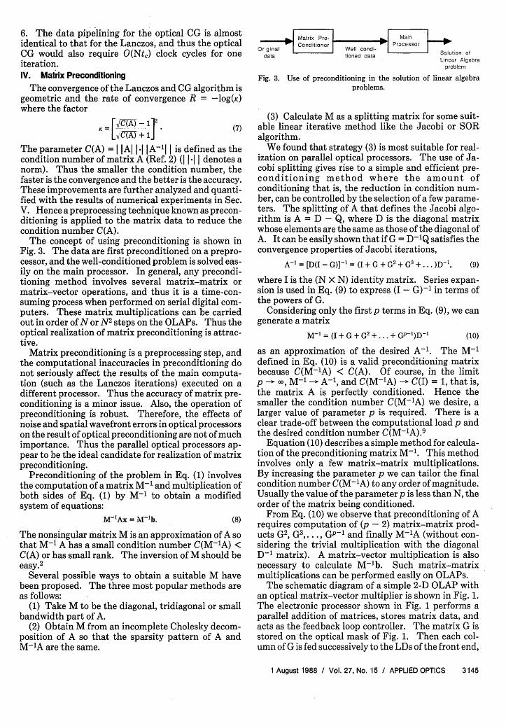
The concept of using preconditioning is shown inFig. 3. The data are first preconditioned on a prepro-cessor, and the well-conditioned problem is solved eas-ily on the main processor. In general, any precondi-tioning method involves several matrix-matrix ormatrix-vector operations, and thus it is a time-con-suming process when performed on serial digital com-puters. These matrix multiplications can be carriedout in order of N or N2 steps on the OLAPs. Thus theoptical realization of matrix preconditioning is attrac-tive.

Matrix preconditioning is a preprocessing step, andthe computational inaccuracies in preconditioning donot seriously affect the results of the main computa-tion (such as the Lanczos iterations) executed on adifferent processor. Thus the accuracy of matrix pre-conditioning is a minor issue. Also, the operation ofpreconditioning is robust. Therefore, the effects ofnoise and spatial wavefront errors in optical processorson the result of optical preconditioning are not of muchimportance. Thus the parallel optical processors ap-pear to be the ideal candidate for realization of matrixpreconditioning.

Preconditioning of the problem in Eq. (1) involvesthe computation of a matrix M-1 and multiplication ofboth sides of Eq. (1) by M-1 to obtain a modifiedsystem of equations:

M-1Ax = M-lb. (8)

The nonsingular matrix M is an approximation of A sothat M-i A has a small condition number C(M-1A) <C(A) or has small rank. The inversion of M should beeasy.2

Several possible ways to obtain a suitable M havebeen proposed. The three most popular methods areas follows:

(1) Take M to be the diagonal, tridiagonal or smallbandwidth part of A.

(2) Obtain M from an incomplete Cholesky decom-position of A so that the sparsity pattern of A andM-1A are the same.

* Matrix Pre- ._ Main_Orgnl Conditioner Welcni Processor 1Original Well cond-Sltino

data tioned data Solution ofLinear Algebra

problem

Fig. 3. Use of preconditioning in the solution of linear algebraproblems.

(3) Calculate M as a splitting matrix for some suit-able linear iterative method like the Jacobi or SORalgorithm.

We found that strategy (3) is most suitable for real-ization on parallel optical processors. The use of Ja-cobi splitting gives rise to a simple and efficient pre-conditioning method where the amount ofconditioning that is, the reduction in condition num-ber, can be controlled by the selection of a few parame-ters. The splitting of A that defines the Jacobi algo-rithm is A = D - Q, where D is the diagonal matrixwhose elements are the same as those of the diagonal ofA. It can be easily shown that if G = D-1 Q satisfies theconvergence properties of Jacobi iterations,

A- = [D(I - G)]V' = (I + G + G + G3 +. . . )D-1 , (9)

where I is the (N X N) identity matrix. Series expan-sion is used in Eq. (9) to express (I - G)-1 in terms ofthe powers of G.

Considering only the first p terms in Eq. (9), we cangenerate a matrix

M- = (I + G + G +. + GP-')D-1 (10)

as an approximation of the desired A-1. The M-1defined in Eq. (10) is a valid preconditioning matrixbecause C(M- 1 A) < C(A). Of course, in the limitp - a, M-1 - A-1 , and C(M-1A) - C(I) = 1, that is,the matrix A is perfectly conditioned. Hence thesmaller the condition number C(M-1A) we desire, alarger value of parameter p is required. There is aclear trade-off between the computational load p andthe desired condition number C(M-1A).9

Equation (10) describes a simple method for calcula-tion of the preconditioning matrix M-1. This methodinvolves only a few matrix-matrix multiplications.By increasing the parameter p we can tailor the finalcondition number C(M-1A) to any order of magnitude.Usually the value of the parameter p is less than N, theorder of the matrix being conditioned.

From Eq. (10) we observe that preconditioning of Arequires computation of (p - 2) matrix-matrix prod-ucts G , G GP-1 and finally M- 1 A (without con-sidering the trivial multiplication with the diagonalD- 1 matrix). A matrix-vector multiplication is alsonecessary to calculate M-1b. Such matrix-matrixmultiplications can be performed easily on OLAPs.

The schematic diagram of a simple 2-D OLAP withan optical matrix-vector multiplier is shown in Fig. 1.The electronic processor shown in Fig. 1 performs aparallel addition of matrices, stores matrix data, andacts as the feedback loop controller. The matrix G isstored on the optical mask of Fig. 1. Then each col-umn of G is fed successively to the LDs of the front end,

1 August 1988 / Vol. 27, No. 15 / APPLIED OPTICS 3145

and the columns of the product G2 would appear suc-cessively on the detector array. Hence the opticalcalculation of the N columns of G2 requires O(N) clockcycles. The columns of G2 are again fed back in paral-lel to the LDs to perform the computation of G3. After(p - 2) sets of such pipelined optical matrix-matrixmultiplications, we obtain the terms, G2, G3 . . ., GP-1in O(pN - 2N) steps.9

When the desired number of the powers of G hasbeen calculated we form the matrix M-1 in the elec-tronic postprocessor in parallel according to Eq. (10).The optical computations of M-1A and M-1 b requireO(N) steps. The whole preconditioning operationthus takes O[(p - 1)N + 1] steps. We notice that onserial digital computers, calculation of all these ma-trix-matrix multiplications require O[(p - )N3]steps.

V. Results of Numerical Experiments

In the numerical experiments carried out, we mod-eled the spatial wavefront errors as random perturba-tions to all matrix and vector data stored on spatiallight modulators during the Lanczos iterations, (forexample, the matrices A and AT on fixed masks). Wesimulated the behavior of the detector noise as time-varying random perturbations to all matrix and vectorproducts computed optically using detector arrays (forexample, the product Ar,). Each sample of the spatialerrors and the detector noise was assumed to be a zero-mean Gaussian random number uncorrelated with oneanother.4 9 We studied the effects of different levels(rms values) of these perturbations on the accuracyand the rate of convergence of the Lanczos iterationsperformed on the ring of OLAPs as shown in Fig. 2.We also studied the improvements in accuracy of thefinal solution with higher levels of polynomial precon-ditioning described in Eq. (10).

A tridiagonal matrix of order (20 X 20) arising fromthe finite difference aproximation to a simple Poissonequation was used for our numerical experiments.The condition number of the matrix A was moderatelylarge C(A) = 958. The matrix was symmetric andpositive definite, and so it satisfied the conditions forthe convergence of both Lanczos and CG algorithms.Also, it was strictly diagonally dominant, and thus wecould use the Jacobi method for preconditioning.

At first, the experiment was conducted with no opti-cal errors to simulate the performance of an ideal opti-cal linear algebra processor. However, the round-offerrors of the digital computer (10-9) limited the accu-racy of iterate x21 to about four places of decimal.Then we studied the effects of a realistic amount ofoptical errors and noises (rms values 10-5) on theperformance of the Lanczos iterations. We noticedthat these optical errors reduced the accuracy of theLanczos iterate x21 to one significant digit only. Whenthe matrix data are preconditioned to a value C(M-1A)= 50 following the strategy in Sec. IV, the Lanczossolution after only ten iterations x, was found to beaccurate to five significant digits. These results aredepicted in Fig. 4. The big improvement in the itera-

0 .1500

-0 .979

-2 .103

-3 .239

-4 .369

-5 .4991.000 5.000 9.000 13.00 17.00 21.00

ITERATION NUMHER ->

Fig. 4. Convergence of the Lanczos algorithm realized on optoelec-tronic processors.

,- UITHOUT PRECONOITIOlIItlG, ITH OPTICRL ERRORS

-2 .993 -

- .333

-5.999 _

ITH PRECONDITIOlING, UITH OPTICRL ERRORS

- .9 -7.99 -6 .99 -5 .99 -4.99LOG (STRNDARD DEVIRTIO) ->

Fig. 5. Improvement in the accuracy of the iterative solution withpreconditioning.

tive solution with preconditioning is shown more clear-ly in Fig. 5 where the inaccuracy in x21 is plotted vs thelevel of errors and noise in the optical processor.

To understand the convergence of the iterations onOLAPs we assume that the rms value of the inaccuracyin the iterate x,, has an upper bound o-, that is,

II Xn-x 1 I S 'r,

where x4 is the accurate value that would be obtainedduring the (n - 1)th iteration if there were no opticalround-off error. Clearly ar is a function of the rmsvalues of spatial errors and detector noise and thematrix data so that t7 increases with an increase in the

3146 APPLIED OPTICS / Vol. 27, No. 15 / 1 August 1988

-. WITHOUT PRECONDITIOllIlIG, UITH OPTICAL ERRORS

WITHOUT PRECONDITIONING, ITHOUT OPTICAL ERRORS

l U - - WITH PRECONDITIONING, UITH OPTICAL ERRORS*_ ~ ~ ~ ------- __- - - _____- --

l

{ l l l

;

rms values. From Ref. 2 we know that for the Lanczosand CG iterations, the distance of the nth iterate fromthe exact solution x of Eq. (1) is given by

I Xn - X I <' K X - |,

where K is defined in Eq. (7) in terms of the conditionnumber C(A). Since we select the initial value x0 = 0,the upper bound in the right-hand side of the aboveequation = K IxI .

Using the last two equations and a result in Ref. 12we have shown that the computational error in theLanczos solution xn on the OLAPs satisfies the follow-ing inequality:

I Xn- XI I< + K X| I

= a[ C(A) + 12 F C (A) |+ r - _ I lixil4xC(A L IC(A) + 1 1-1

(11)

Because of the inequalities of matrix norms, the upperbound to the computational error described in Eq. (11)is conservative. However, it provides an estimate ofhow the hardware and the data affect the iterations.In Eq. (11) we observe that the errors in the iterativesolution have two components. One part is indepen-dent of n and thus represents the noise floor, the inac-curacy that is determined by the hardware errors a andthe condition number C(A). The other part decreaseswith the number of iteration n because K < 1. Figure 4clearly brings out the existence of these two compo-nents of inaccuracy and shows that both componentsare strong functions of the condition number of thematrix. Therefore, the inaccuracies in xn decrease asthe condition number and optical errors are decreased.The only way of reducing the condition number is themethod of preconditioning we discussed. The opticalerrors can only be reduced through careful design andselection of better components.

Thus we notice that preconditioned Lanczos algo-rithm works reasonably well on a ring of analog anddigital OLAPs.

VI. Technique for Manipulation of Large SparseMatrices on 2-D Spatial Light Modulators

The practical optical linear algebra processorsshould be capable of providing a static or dynamicstorage of large sparse matrices and of multiplyingsuch matrices with other matrices. In this section, anew technique for storing large banded or block-diago-nal matrices on 2-D spatial light modulators excludingmost of the insignificant zeros and the optical parallelmultiplications of these matrices by vectors are de-scribed. Special attention is paid to the use of theavailable magnetooptic or liquid crystal spatial lightmodulators.

The essence of this technique is the storage of thenonzero diagonals of the sparse matrix as the horizon-tal rows of a 2-D spatial light modulator as shown inFig. 6. We require only an (M X N) spatial lightmodulator to store a sparse matrix of dimension(N X N) with a total of M significant diagonals (M << N).The technique of optically multiplying this stored ma-

Fig. 6. Scheme for

LED array

0 a12 aa ; 23

a22

a2 ~a 2-D SLM

El F- / Detector array

storage and vector multiplication of a tridia-gonal sparse matrix.

- ~ ~~~~ a7 a,

12 23 34

a a22 a33

a21 a32

trix ith n (N 1) eos als aeitdi i.6

a65 ~~54 43

a6e a55 ah

7 ae a45

a aa a. a

a 76 a8 a9

Fig. 7. Folded storage of a tridiagonal (9 X 9) matrix on a (9 X 5)spatial light modulator array.

trix with an (N X 1) vector is also depicted in Fig. 6.Each element of the vector is represented by the inten-sity of a point modulator whose light uniformly illumi-nates one column of our (M X N) storage. The lightleaving the spatial light modulator is mapped by askewed array of optical fiber'bundles onto the N ele-ments of a photodetector array. Thus, in this tech-nique, the effective angle between the point modulatorand detector arrays depends on the bandwidth M. Inthe standard 2-D optical matrix-vector multiplicationschemes, the point modulator and detector arrays arekept at right angles.

Since the dimension N is large, the diagonals can befolded to fit all the data in a 2-D spatial light modulatorin which the number of available columns is <N. Thefolded storage of a tridiagonal (9 X 9) matrix on a(9 X 5) array with two extra columns (necessary forfolding) on two sides is shown in Fig. 7. Similarly, itcan be shown that a pentadiagonal (350 X 350) sparsematrix with each element represented by an eight-bitbinary number can be fitted easily on an (128 X 128)Sight-Mod magnetooptic spatial light modulator arraymade by Semetex Corp.

With appropriate mappings, this technique can beapplied to the dynamic storage of matrices in multi-channel acoustooptic cells. Useful guidelines on par-titioning a large sparse matrix for optical processing

1 August 1988 / Vol. 27, No. 15 / APPLIED OPTICS 3147

also evolve from this technique. We notice that ourfolded storage scheme increases the complexity of op-tical mapping; the speed of executing a matrix multi-plication is not degraded.

VII. Epilogue

In this paper, we have described a new scheme for apipelined realization of the Lanczos and the CG algo-rithms on a ring of parallel OLAPs. We have dis-cussed the design of an optical preconditioning prepro-cessor that can help the execution of the iterativealgorithms on the main ring. We have described howthese algorithms would behave on such a ring ofOLAPs. A design of such an involved optical multi-processor is in progress in our laboratory to verify theobservations and conjectures presented in this paper.

The scheme of realization of the Lanczos and CGalgorithms presented can be easily adopted for parallelsystolic and wavefront processors. Only we have tochange the way the matrix-vector and vector-vectormultiplications are executed. The data flow and in-terconnection of the processors should be the same asthat shown in Fig. 2.

We are grateful to P. Paparao for his help with thenumerical experiments. Many discussions with P.Banerjee of Syracuse University are acknowledged.Part of this research is supported by NSF grant EET-8707863.

Appendix: Conjugate Gradient Algorithm

The conjugate gradient algorithm can be stated inmany ways.2 10 A form suitable for parallel realizationon vector processors runs as follows:Step (1) Define vectors x_1 = r 1 = 0.Step (2) Select the initial choice x0 = 0. Let P1 = 1.

Calculate r = b - Axo = b.Step (3) For n = 0,1,2,. . ., calculate the scalars.

n= 1 - Pn+l,

=n+1 =yn+lPn+l,

frnAr.1

=1 1 - Yn+ i rn ]-1anl cnrn-Parn-i}Then update the new estimate Xn+ = an+lrn + Pn+lXn+ fn+lxn-, and the residual vector rn+l = -an+l(Arn)+ Pn+lrn + 1n+irn-1-Step (4) If the norm of the residuals trn,rn} < E stop,

else continue step (3).

References1. D. Casasent, "Acoustooptic Linear Algebra Processors: Archi-

tectures, Algorithms, and Applications," Proc. IEEE 72, 831(1984).

2. G. Golub and C. VanLoan, Matrix Computations (Johns Hop-kins U. P., Baltimore, 1983).

3. H. Chen, T. Sarkar, S. Dianat, and J. Brule, "Adaptive SpectralEstimation by the Conjugate Gradient Method," IEEE Trans.Acoust. Speech Signal Process. ASSP-34, 272 (1986).

4. D. Casasent and A. Ghosh, "Optical Linear Algebra Processors:Noise and Error-Source Modeling," Opt. Lett. 10, 252 (1985).

5. D. Psaltis and R. Athale, "High Accuracy Computations withLinear Analog Optical Systems: A Critical Study," Appl. Opt.25, 3071 (1986).

6. A. Ghosh, "Realization of Conjugate Gradient Algorithms onOptical Linear Algebra Processors," Appl. Opt. 26, 611 (1987).

7. S. Welstead, "Analog Algorithms for Optical Signal Processing,"in Proceedings, Twentieth Asilomar Conference on Signals,Systems and Computers (IEEE Computer Society Press, 1987),pp. 536-540.

8. A. McAulay, "Conjugate Gradients on Optical Crossbar Inter-connected Multiprocessor," J. Parallel Distributed Process. toappear (1988).

9. A. Ghosh and P. Paparao, "Matrix Preconditioning: A RobustOperation for Optical Linear Algebra Processors," Appl. Opt.26,2734 (1987); "Performance Analysis of Matrix Precondition-ing Algorithms on Parallel Optical Processors," J. Opt. Soc. Am.A 5, 39 (1988).

10. L. Hageman and D. Young, Applied Iterative Methods (Aca-demic, New York, 1981).

11. D. Psaltis, D. Casasent, and M. Carlotto, "Iterative Color-Multi-plexed Electrooptical Processor," Opt. Lett. 4, 348 (1979).

12. E. Filippovich, "The Effect of Rounding Errors in IterationalProcesses," Zh. Vychisl. Mat. Mat. Fiz. 25, 973 (1985).

F. T. Stone, AT&T Bell Laboratories-Allentown, photographed byW. J. Tomlinson, Bellcore-Red Bank, at the Conference on OpticalFiber Communications, New Orleans, January 1988.

3148 APPLIED OPTICS / Vol. 27, No. 15 / 1 August 1988