LUND UNIVERSITY

PO Box 117221 00 Lund+46 46-222 00 00

Realistic tissue dosimetry models using Monte Carlo simulations. Applications forradionuclide therapies

Larsson, Erik

2011

Link to publication

Citation for published version (APA):Larsson, E. (2011). Realistic tissue dosimetry models using Monte Carlo simulations. Applications forradionuclide therapies. Department of Medical Radiation Physics, Clinical Sciences, Lund, Lund University.

General rightsUnless other specific re-use rights are stated the following general rights apply:Copyright and moral rights for the publications made accessible in the public portal are retained by the authorsand/or other copyright owners and it is a condition of accessing publications that users recognise and abide by thelegal requirements associated with these rights. • Users may download and print one copy of any publication from the public portal for the purpose of private studyor research. • You may not further distribute the material or use it for any profit-making activity or commercial gain • You may freely distribute the URL identifying the publication in the public portal

Read more about Creative commons licenses: https://creativecommons.org/licenses/Take down policyIf you believe that this document breaches copyright please contact us providing details, and we will removeaccess to the work immediately and investigate your claim.

Realistic tissue dosimetry models using Monte Carlo simulations

Applications for radionuclide therapies

Erik Larsson

Department of Medical Radiation Physics Clinical Sciences, Lund

Lund University, Sweden

ii

Copyright © Erik Larsson 2011 Department of Medical Radiation Physics Clinical Sciences, Lund Lund University SE-221 85 Lund Sweden ISBN 978-91-7473-193-4 Printed in Sweden by Media-Tryck, Lund University, Lund 2011

iii

"Simulation is better than reality" Richard W. Hamming

iv

v

ABSTRACT

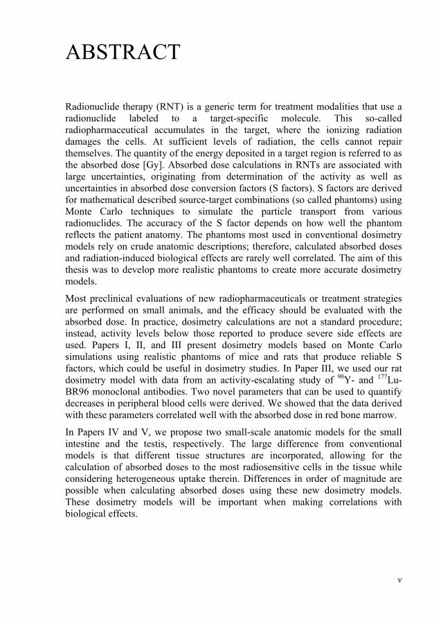
Radionuclide therapy (RNT) is a generic term for treatment modalities that use a radionuclide labeled to a target-specific molecule. This so-called radiopharmaceutical accumulates in the target, where the ionizing radiation damages the cells. At sufficient levels of radiation, the cells cannot repair themselves. The quantity of the energy deposited in a target region is referred to as the absorbed dose [Gy]. Absorbed dose calculations in RNTs are associated with large uncertainties, originating from determination of the activity as well as uncertainties in absorbed dose conversion factors (S factors). S factors are derived for mathematical described source-target combinations (so called phantoms) using Monte Carlo techniques to simulate the particle transport from various radionuclides. The accuracy of the S factor depends on how well the phantom reflects the patient anatomy. The phantoms most used in conventional dosimetry models rely on crude anatomic descriptions; therefore, calculated absorbed doses and radiation-induced biological effects are rarely well correlated. The aim of this thesis was to develop more realistic phantoms to create more accurate dosimetry models.

Most preclinical evaluations of new radiopharmaceuticals or treatment strategies are performed on small animals, and the efficacy should be evaluated with the absorbed dose. In practice, dosimetry calculations are not a standard procedure; instead, activity levels below those reported to produce severe side effects are used. Papers I, II, and III present dosimetry models based on Monte Carlo simulations using realistic phantoms of mice and rats that produce reliable S factors, which could be useful in dosimetry studies. In Paper III, we used our rat dosimetry model with data from an activity-escalating study of 90Y- and 177Lu-BR96 monoclonal antibodies. Two novel parameters that can be used to quantify decreases in peripheral blood cells were derived. We showed that the data derived with these parameters correlated well with the absorbed dose in red bone marrow.

In Papers IV and V, we propose two small-scale anatomic models for the small intestine and the testis, respectively. The large difference from conventional models is that different tissue structures are incorporated, allowing for the calculation of absorbed doses to the most radiosensitive cells in the tissue while considering heterogeneous uptake therein. Differences in order of magnitude are possible when calculating absorbed doses using these new dosimetry models. These dosimetry models will be important when making correlations with biological effects.

vi

Summary in Swedish

Vid radionuklidterapi används ett radioaktivt läkemedel för behandling av vissa sjukdomar, bl.a. struma och vissa tumörsjukdomar. En radionuklidmärkt målspecifik molekyl administreras till patienten och läkemedlet transporteras via blodomloppet till det sjuka området där molekylens egenskaper gör att läkemedlet ansamlas. Den joniserande strålningen som sänds ut från läkemedlet ger upphov till skador på DNA i cellkärnan. Desto fler skador som inträffar på DNA, desto mindre är chansen att cellen ska kunna reparera skadorna vilket slutligen leder till att cellen slutar fungera eller till och med dör. Måttet som används för att bestämma den deponerade strålningsenergin per massenhet är absorberad dos [Gy]. Att beräkna den absorberade dosen är viktigt för att kunna undvika allvarliga bieffekter av strålningen och därmed kunna optimera behandlingseffekten. Före en ny behandling eller behandlingsstrategi testas på människor utförs ofta studier på råttor och möss. Utvärderingen av behandlingseffekt bör då korreleras mot absorberad dos.

Ett led att beräkna absorberad dos ligger i att bestämma var den emitterade energin deponeras. Denna transport av partiklarna kan inte beräknas analytiskt, så istället simuleras transporten av partiklarna i ett datorprogram enligt den så kallade Monte Carlo metoden. För att kunna simulera partiklarnas transport krävs en matematisk modell som beskriver anatomin. De konventionella dosimetrimodellerna använder sig av en väldigt förenklad representation av organen och dess inbördes läge, vilket i slutändan innebär stora osäkerheter i absorberad dos. Detta resulterar i svaga samband mellan beräknad absorberad dos och en studerad biologisk effekt. Målet med denna avhandling har varit att använda sig av realistiska beskrivningar av anatomin för att utveckla nya noggrannare dosimetrimodeller.

I de tre första arbetena presenteras dosimetrimodeller som bygger på anatomiskt realistiska matematiska modeller av mus och råtta, vilka kan användas vid dosimetristudier. I arbete III beräknas den absorberade dosen till benmärg hos råtta vid en radionuklidterapi med antikroppar och korreleras med observerad nedgång i cirkulerande blodceller. Två nya metoder att kvantifiera denna biologiska effekt presenteras och visar sig ge en starkare korrelation än tidigare metoder.

I de två sista arbetena presenteras två dosimetrimodeller, en för testikel och en för tunntarmens vägg. De konventionella metoderna ger en medelabsorberad dos till hela vävnaden, meden dessa nya modeller tar hänsyn till vävnadens cellstruktur och var de mest strålkänsliga cellerna finns. Detta innebär även att man kan ta hänsyn till hur aktiviteten fördelar sig i organet. Beroende på vilken dosimetrimodell som används, så blir det ofta stora skillnader i beräknad absorberad dos. Med dessa nya modeller får vi en noggrannare bestämning av absorberad dos för de strålkänsliga cellerna och hoppas därmed finna starkare samband med biologiska respons.

vii

List of Publications

This thesis consists of the following publications, which are referred to with Roman numerals I-V.

I. Erik Larsson, Sven-Erik Strand, Michael Ljungberg, Bo-Anders Jönsson. Mouse S-factors based on Monte Carlo simulations in the anatomical realistic Moby phantom for internal dosimetry. Cancer Biotherapy and Radiopharmaceuticals. 2007;22(3):438-442.

II. Erik Larsson, Michael Ljungberg, Sven-Erik Strand, Bo-Anders Jönsson. Monte Carlo calculations of absorbed doses in tumours using a modified MOBY mouse phantom for pre-clinical dosimetry studies. Acta Oncologica. 2011;50(6):973-980.

III. Erik Larsson, Michael Ljungberg, Linda Mårtensson, Rune Nilsson, Jan Tennvall, Sven-Erik Strand, Bo-Anders Jönsson. Use of Monte Carlo simulations with a realistic rat phantom for examining the correlation between hematopoietic system response and red marrow absorbed dose in Brown Norway rats undergoing radionuclide therapy with 177Lu- and 90Y-BR96 mAbs. Submitted to Medical Physics.

IV. Erik Larsson, Bo-Anders Jönsson, Lena Jönsson, Michael Ljungberg, Sven-Erik Strand. Dosimetry calculations on a tissue level by using the MCNP4c2 Monte Carlo code. Cancer Biotherapy and Radiopharmaceuticals. 2005;20(1):85-91.

V. Erik Larsson, Suaad A. Meerkhan, Sven-Erik Strand, Bo-Anders Jönsson. Small-scale anatomic model for testicular radiation dosimetry for radionuclides localized in the human testes. Journal of Nuclear Medicine. In press January 2012.

Reprinting of the papers was kindly permitted by Mary Ann Liebert, Inc., publishers (I and IV), Informa Healthcare (II), and the Society of Nuclear Medicine (V).

viii

Abbreviations

3D Three-dimensional 4D Four-dimensional AF Absorbed fraction ARG Autoradiography BED Biological effective dose BM Bone marrow BN Brown Norway (rat strain) CT Computed tomography DSB Double-strand break HCT Hematocrit ICRP International Commission on Radiological Protection ITS Integrated TIGER Series LET Linear energy transfer mAb Monoclonal antibody MC Monte Carlo MCNP Monte Carlo N-Particles MCNPX Monte Carlo N-Particles eXtended µCT Micro computed tomography µPET Micro positron emission tomography MRI Magnetic resonance imaging µSPECT Micro single photon emission computed tomography NM Nuclear medicine NURBS Non-uniform rational B-spline pdf Probability density function PET Positron emission tomography PM Polygonal mesh RBC Red blood cells RIT Radioimmunotherapy RM Red marrow RMBLR Red marrow-to-blood ratio RNT Radionuclide therapy SI Small intestine SPECT Single-photon emission computed tomography WBC White blood cells

ix

Table of Contents

1. Introduction 1

1.1 Radionuclide therapy 1

1.2 Dosimetry in nuclear medicine 2

1.3 Correlations between dosimetry and biological effect 3

1.4 Aims of the work presented in this thesis 5

2. Internal dosimetry 7

2.1 MIRD-formalism 7

2.2 Small-scale dosimetry 10

2.3 Microdosimetry 12

2.4 Bone marrow dosimetry 12

2.4.1 Blood method 13

2.4.2 Red marrow dosimetry models 14

3. Radiobiology 16

3.1 Bone Marrow 16

3.2 Small Intestines 18

3.3 Testis 19

4. Radionuclides 21

5. Imaging 24

5.1 Small-animal systems 24

5.2 Autoradiography 26

6. Phantoms 28

6.1 Human whole-body phantoms 28

x

6.2 Small-animal phantoms 32

6.3 Small-scale tissue dosimetry models 34

6.3.1 Small intestine 34

6.3.2 Testis 35

7. The Monte Carlo method 37

7.1 Introduction 37

7.2 Photon transport 38

7.3 Electron transport 39

7.4 Variance reduction 40

7.5 General Monte Carlo codes 41

7.6 The MCNP5/MCNPX code package 42

7.6.1 Photons 43

7.6.2 Electrons 43

7.6.3 Tallies 46

7.6.4 Use of MCNP in this thesis 46

8. Summary of Papers 48

9. Conclusion 53

10. Future/Vision 54

Acknowledgements 56

References 57

1

1. Introduction

Nuclear medicine (NM) is a generic term for diagnostics or therapies involving pure radionuclides or tracer amounts of specific molecules labeled with radionuclides—so-called radiopharmaceuticals. In contrast to imaging techniques such as conventional X-ray, CT, ultrasound, or MRI, in which images usually reflect anatomy, the parameters studied in NM are purely physiological and depend on the chemical and biological properties of the radiopharmaceutical used. One of the most commonly performed imaging techniques in NM is myocardial SPECT for the diagnosis of ischemia or infarct within the heart muscle. A radiopharmaceutical is injected intravenously, and the uptake in the myocardium is reflected in the regional blood flow. The emitted photons are detected using a scintillation camera that creates an image of the radionuclide distribution. From measurements taken in multiple views by rotating the scintillation camera, tomographic images can be reconstructed. A two-part study can be performed in which a patient’s heart is examined at rest and then under stress from either exercise or the administration of a drug, e.g., adenosine. Regional areas that show decreased uptake in the stress images correspond to ischemia, whereas a decrease that shows in both the rest and the stress images is likely an infarct. Another common NM study involves bone scintigraphy, in which images show bone metabolism (i.e., bone metastasis or bone fractures). 18F-FDG (flurodeoxyglucose) is a glucose analog that has a large uptake in brain, heart, and, most important, many cancers. The interest in PET examinations with 18F-FDG for tumor detection and staging and other PET radiopharmaceuticals has increased the number of available PET systems.

1.1 Radionuclide therapy

Radionuclide therapy (RNT) is a treatment modality that involves radionuclides in ion form or attached to a targeting molecule. The first compound used for this type of therapy was 32P-phosphate, which has been used for more than 70 years. About 30% of the 32P-phosphate accumulates permanently in mineral bone, where radiation delivers a significant absorbed dose to the red marrow (RM). Initially, 32P-phosphate was used as a treatment for leukemia but has for the last 30 years been an established treatment of polycythemia vera (a rare blood disease characterized by an elevation in red blood cells [RBCs]) and essential

2

thrombocythemia (increased levels of platelets). The aim of this treatment is to suppress rather than eradicate hyperproliferative cell lines (1).

The majority of the approximately 2800 RNTs administered in Sweden in 2009 were treatments for hyperthyroidism with 131I-NaI. Hyperthyroidism is an illness in which the thyroid overproduces the hormones T3 (triiodothyronine) and/or T4 (thyroxine), which regulate metabolism and the function of several other systems in the organ. Iodine is naturally involved in the synthesis of T3 and T4. The same radiopharmaceutical is also often used for the treatment of thyroid cancer because the malignant cells inherit the ability to absorb iodine. Other clinically used RNTs are 89SrCl, 223RaCl, and 153Sm-EDTMP (ethylene diamine tetramethylene phosphonate), which are used mainly for palliative treatments of bone metastasis.

Several monoclonal antibodies (mAbs) are available for radioimmunotherapy (RIT). These antibodies are large proteins that have binding sites with an affinity for a specific antigen that is expressed on the cell surface—a tumor cell, for example. At present, 2 commercially approved RIT agents are available: 90Y-ibritumomab tiuxetan (Zevalin®; Biogen-Idec Pharmaceuticals, San Diego, CA; approved by the U.S. Food and Drug Administration in 2002) and 131I-tositumomab (BEXXAR®, GlaxoSmithKline, Philadelphia, PA; approved in 2003). These mAbs are usually used as treatment of non-Hodgkin’s B-cell lymphoma. Because they are CD20 positive—an antigen usually expressed in both malignant and in different phases of maturation in natural B-cells but not B-cell progenitors and early pro B-cells—the radiation is accumulated in the lymphoma and circulating malignant cells, which can then be replaced by new, healthy B-cells produced by the progenitors (2).

An RNT treating modality that has received increased attention is peptide receptor radionuclide therapy (PRRT). The most used radiopharmaceuticals in this group have been [90Y-DOTA0, Tyr3]-octreotide (DOTATOC) (3, 4) and [177Lu-DOTA0-Tyr3]-octeotate (5, 6). These are somatostatin analogues, peptide hormones that regulate the endocrine system. The number of somatostatin receptors is overexpressed on many neuroendocrine tumors, allowing a high tumor-to-normal activity ratio and the opportunity to deliver high absorbed doses to the tumors.

1.2 Dosimetry in nuclear medicine

The time-activity kinetic behavior of a radiopharmaceutical in the organs of interest must be determined to calculate the absorbed dose in NM, and from this information, a dosimetry method that models the physical properties of the emitted radiation must be used. As the next chapters describe, this task may be rather complicated. Dosimetry studies are not performed regularly for clinically approved radiopharmaceuticals for diagnostic imaging; however, before radiopharmaceuticals are clinically approved, dosimetry investigations must be

3

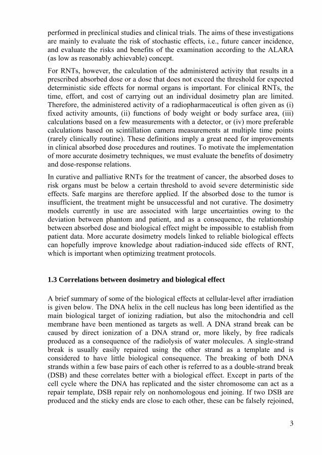
performed in preclinical studies and clinical trials. The aims of these investigations are mainly to evaluate the risk of stochastic effects, i.e., future cancer incidence, and evaluate the risks and benefits of the examination according to the ALARA (as low as reasonably achievable) concept.

For RNTs, however, the calculation of the administered activity that results in a prescribed absorbed dose or a dose that does not exceed the threshold for expected deterministic side effects for normal organs is important. For clinical RNTs, the time, effort, and cost of carrying out an individual dosimetry plan are limited. Therefore, the administered activity of a radiopharmaceutical is often given as (i) fixed activity amounts, (ii) functions of body weight or body surface area, (iii) calculations based on a few measurements with a detector, or (iv) more preferable calculations based on scintillation camera measurements at multiple time points (rarely clinically routine). These definitions imply a great need for improvements in clinical absorbed dose procedures and routines. To motivate the implementation of more accurate dosimetry techniques, we must evaluate the benefits of dosimetry and dose-response relations.

In curative and palliative RNTs for the treatment of cancer, the absorbed doses to risk organs must be below a certain threshold to avoid severe deterministic side effects. Safe margins are therefore applied. If the absorbed dose to the tumor is insufficient, the treatment might be unsuccessful and not curative. The dosimetry models currently in use are associated with large uncertainties owing to the deviation between phantom and patient, and as a consequence, the relationship between absorbed dose and biological effect might be impossible to establish from patient data. More accurate dosimetry models linked to reliable biological effects can hopefully improve knowledge about radiation-induced side effects of RNT, which is important when optimizing treatment protocols.

1.3 Correlations between dosimetry and biological effect

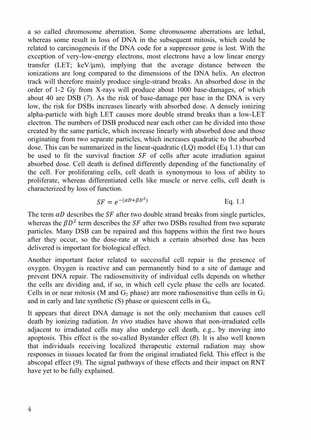
A brief summary of some of the biological effects at cellular-level after irradiation is given below. The DNA helix in the cell nucleus has long been identified as the main biological target of ionizing radiation, but also the mitochondria and cell membrane have been mentioned as targets as well. A DNA strand break can be caused by direct ionization of a DNA strand or, more likely, by free radicals produced as a consequence of the radiolysis of water molecules. A single-strand break is usually easily repaired using the other strand as a template and is considered to have little biological consequence. The breaking of both DNA strands within a few base pairs of each other is referred to as a double-strand break (DSB) and these correlates better with a biological effect. Except in parts of the cell cycle where the DNA has replicated and the sister chromosome can act as a repair template, DSB repair rely on nonhomologous end joining. If two DSB are produced and the sticky ends are close to each other, these can be falsely rejoined,

4

a so called chromosome aberration. Some chromosome aberrations are lethal, whereas some result in loss of DNA in the subsequent mitosis, which could be related to carcinogenesis if the DNA code for a suppressor gene is lost. With the exception of very-low-energy electrons, most electrons have a low linear energy transfer (LET; keV/μm), implying that the average distance between the ionizations are long compared to the dimensions of the DNA helix. An electron track will therefore mainly produce single-strand breaks. An absorbed dose in the order of 1-2 Gy from X-rays will produce about 1000 base-damages, of which about 40 are DSB (7). As the risk of base-damage per base in the DNA is very low, the risk for DSBs increases linearly with absorbed dose. A densely ionizing alpha-particle with high LET causes more double strand breaks than a low-LET electron. The numbers of DSB produced near each other can be divided into those created by the same particle, which increase linearly with absorbed dose and those originating from two separate particles, which increases quadratic to the absorbed dose. This can be summarized in the linear-quadratic (LQ) model (Eq 1.1) that can be used to fit the survival fraction of cells after acute irradiation against absorbed dose. Cell death is defined differently depending of the functionality of the cell. For proliferating cells, cell death is synonymous to loss of ability to proliferate, whereas differentiated cells like muscle or nerve cells, cell death is characterized by loss of function. = ( ) Eq. 1.1

The term describes the after two double strand breaks from single particles, whereas the term describes the after two DSBs resulted from two separate particles. Many DSB can be repaired and this happens within the first two hours after they occur, so the dose-rate at which a certain absorbed dose has been delivered is important for biological effect.

Another important factor related to successful cell repair is the presence of oxygen. Oxygen is reactive and can permanently bind to a site of damage and prevent DNA repair. The radiosensitivity of individual cells depends on whether the cells are dividing and, if so, in which cell cycle phase the cells are located. Cells in or near mitosis (M and G2 phase) are more radiosensitive than cells in G1 and in early and late synthetic (S) phase or quiescent cells in G0.

It appears that direct DNA damage is not the only mechanism that causes cell death by ionizing radiation. In vivo studies have shown that non-irradiated cells adjacent to irradiated cells may also undergo cell death, e.g., by moving into apoptosis. This effect is the so-called Bystander effect (8). It is also well known that individuals receiving localized therapeutic external radiation may show responses in tissues located far from the original irradiated field. This effect is the abscopal effect (9). The signal pathways of these effects and their impact on RNT have yet to be fully explained.

5

In this thesis we investigate 3 highly radiosensitive tissues: the red bone marrow (Paper III), small intestine (Paper IV), and testis (Paper V). A common feature is that these tissues include rapidly dividing stem cells and are therefore considered highly radiosensitive. The radiobiology for these tissues is explained in more detail in Chapter 3.

1.4 Aims of the work presented in this thesis Our focus has been the development of more realistic dosimetry models. In the commonly used dosimetry models for humans, the dimensions of the organs are so large that electrons can be considered locally absorbed. In the work presented herein, we use small-scale models of small animals like mice and rats or small-scale anatomic dosimetry models of tissues with differentiated cell architecture. A common thread within these models is the importance of having realistic geometric descriptions of the anatomy so that the electron transport and interaction sites can be simulated with high accuracy.

Paper I: This paper describes the development of a dosimetry model based on a realistic anatomic representation of a mouse (from the MOBY software). A program that allowed the Monte Carlo (MC) code MCNPX to use voxel-based information was developed for the purpose of deriving S factors for the mouse. These results were compared to those obtained from an EGS4-based MC code. The S factors were also compared to data published for other dosimetry models.

Paper II: This paper is a continuation of the work described in Paper I. Subcutaneous tumor models were developed to investigate the dependence of the absorbed dose to the tumor and other organs on the tumor size and location and parameters related to the kinetics of the radiopharmaceutical. An improved version of the MOBY software was used that allowed for separation of bone marrow (BM) regions. The study included 3 mouse sizes and tumors of varying size in 4 locations.

Paper III: In this work we used the ROBY software to develop a dosimetry model for a rat in a manner similar to that described in Paper II. The aim was to use published rat kinetic data of 111In-BR96-mAbs (10) together with an activity-escalating study of 90Y- and 177Lu-BR96-mAbs (11) in rats to calculate the absorbed doses. Decreases in white blood cells (WBCs), platelets, and body weight were evaluated using various parameters for quantification. Two of these parameters were the drop—the decrease from the start value at nadir normalized to the start value—and the recovery time. We also defined 2 additional parameters that describe the area loss in a time-blood cell count curve compared to untreated animals or a baseline value.

6

Paper IV: The aim of this study was to develop an MCNP4c2 code for the small-scale anatomic intestinal dosimetry model previously described by Jönsson et al. (12) and to improve that model. The absorbed dose to the radiosensitive crypt cells was calculated instead of an average absorbed dose to the whole intestinal wall.

Paper V: There has been a lack of detailed dosimetry models of the testicles on a cellular level. The aim of this work was to develop such a small-scale dosimetry model with which to calculate S factors for several source-target configurations within testicular tissue, therefore allowing for an accurate calculation of the absorbed dose to the highly radiosensitive spermatogonia.

7

2. Internal dosimetry

2.1 MIRD-formalism

The absorbed dose is defined as the mean energy imparted ̅ to matter of mass and is expressed with the unit Gy [J/kg] (13).

= ̅ Eq. 2.1

In dosimetry for diagnostic and therapeutic NM, it is the mean absorbed dose to any tissue that constitutes the basis for the general MIRD (medical internal radiation dose) formalism (14, 15), now described as the following:

( ← , ) = ( , ) · ( ← , ) Eq. 2.2

Equation 2.2 explains that the mean absorbed dose rate at time to the target region from source region is the product of the time-dependent activity in the source region ( , ) and a dose conversion factor (S factor) specific for any type of radiation, energy, and source-target combination. The source activity is supposed to be homogenously distributed in the source region, and the atomic composition and mass density of the mediums are supposed to be distributed homogenously in the source and target regions.

To calculate the absorbed dose, the sum from all contributing source regions and integration over the time interval 0, ] is calculated. The total absorbed dose to the target can then be expressed as follows:

( , ) = ( , ) = ( , ) · ( ← , ) Eq. 2.3

Equations 2.2 and 2.3 show the time-dependent MIRD formalism. In some situations, the S factor cannot be treated as a constant value—such as the absorbed dose to tumors (16), in which the mass can decrease or increase during the time the absorbed dose is delivered. The S factors used in this thesis were considered constant during the integration time. Equation 2.3 can then be simplified to the following:

8

( , ) = ( , ) · ( ← ) =

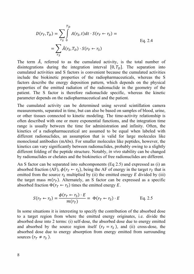
= ( , ) · ( ← ) Eq. 2.4

The term , referred to as the cumulated activity, is the total number of disintegrations during the integration interval 0, ]. The separation into cumulated activities and S factors is convenient because the cumulated activities include the biokinetic properties of the radiopharmaceuticals, whereas the S factors describe the energy deposition pattern, which depends on the physical properties of the emitted radiation of the radionuclide in the geometry of the patient. The S factor is therefore radionuclide specific, whereas the kinetic parameter depends on the radiopharmaceutical and the patient. The cumulated activity can be determined using several scintillation camera measurements, separated in time, but can also be based on samples of blood, urine, or other tissues connected to kinetic modeling. The time-activity relationship is often described with one or more exponential functions, and the integration time range is usually between the time for administration and infinity. Often, the kinetics of a radiopharmaceutical are assumed to be equal when labeled with different radionuclides, an assumption that is valid for large molecules like monoclonal antibodies (mAbs). For smaller molecules like peptides, however, the kinetics can vary significantly between radionuclides, probably owing to a slightly different folding of the peptide structure. Notably, in vivo stability can be changed by radionuclides or chelates and the biokinetics of free radionuclides are different.

An S factor can be separated into subcomponents (Eq 2.5) and expressed as (i) an absorbed fraction (AF), ( ← ), being the AF of energy in the target that is emitted from the source multiplied by (ii) the emitted energy divided by (iii) the target mass ( ). Alternately, an S factor can be expressed as a specific absorbed fraction Φ( ← ) times the emitted energy .

( ← ) = ( ← ) ·( ) = Φ( ← ) ·

Eq. 2.5

In some situations it is interesting to specify the contribution of the absorbed dose to a target region from where the emitted energy originates, i.e. divide the absorbed dose into 2 terms: (i) self-dose, the absorbed dose due to energy emitted and absorbed by the source region itself ( = ), and (ii) cross-dose, the absorbed dose due to energy absorption from energy emitted from surrounding sources ( ≠ ).

9

To calculate an S factor, the absorbed energy in the target region must be determined. This can be determined by a convolution procedure using precalculated dose point kernels (17). This method is fast and, in many cases, sufficiently accurate. More complex non-homogeneous geometries of different atomic compositions and densities require a full Monte Carlo simulation to obtain accurate results. In such cases, a large number of decays must be simulated. The entire energy spectra of all emitted particles and yields must be included, and the energy deposition in the target regions must be scored. The accuracy of the simulated S factors can be well within a few percentages for certain geometric representations of the anatomy (phantoms). How well a phantom matches the anatomy of a patient determines the accuracy of the S factor for that patient.

When calculating the absorbed dose to a patient based on a distribution from clinical SPECT images, it is questionable whether a full simulation of the electrons must be considered. The electron ranges are often small compared to the SPECT voxels, so much time is spend on simulating a particle within the source voxel. The SPECT image is also affected by the spatial resolution (on the order of 10-15 mm full width at half maximum) of the SPECT system, which blurs the image of the activity distribution. This blurring is larger than the electron range for all radionuclides used in RNT, which implies that a SPECT image may very well show the absorbed energy distribution with sufficient accuracy (18). Because photons have long mean-free path lengths, however, they must be considered explicitly and could be important for some radionuclides, such as radionuclides used for imaging or 131I, which is widely used in RNT. When working with small-scale models or high-resolution imaging systems, electron transport must be modeled.

The MIRD formalism is often criticized as being valid only for average organ absorbed doses, but this criticism is not entirely justified. This criticism is based on the less than realistic stylized MIRD phantoms for organ doses and their corresponding tabulated S values. The MIRD formalism is, however, valid for arbitrary source and target regions, and thus is not limited to average organ absorbed doses but can also be used on a voxel-to-voxel level or on a small-scale level, as in Papers IV and V. The MIRD formalism is valid until the source and target volumes are so small that the statistical fluctuation of the decays and the energy deposition increase, requiring a microdosimetric approach.

When calculating an average organ absorbed dose in humans, charged particles are often considered to be locally absorbed owing to their short ranges. This assumption leads to simpler and faster simulations and allows the scaling of the electron and photon parts of the S value for self-dose with a more accurate organ mass (19, 20), as shown in equations 2.6 and 2.7.

= · Eq. 2.6

10

= · / Eq. 2.7

In Paper IV, we develop a small-scale dosimetry model for the small intestine (SI). Conventional ICRP (21) and MIRD (14) models of the intestines considered the wall as the risk organ and only the intestinal contents as the source of radiation. The contribution of the absorbed dose to the wall from photons was approximated by the average absorbed dose of both contents and wall. The absorbed dose from charged particles was approximated by the “one-half assumption,” in which the specific absorbed fraction Φ from non-penetrating radiation is given by

Φ(r ← r ) = 12 · ·

Eq. 2.8

where is the mass of the intestinal contents, and the factor represents the penetration of the radiation to the radiosensitive cells in the wall and is considered to be 1 for electrons and 0.01 for α-particles (21).

Since the publication of Paper IV, ICRP has revised their dosimetry model for the human alimentary tract (22). Their SI-models are derived for different age-categories, and are based on a 120-280 cm long cylinder with an age-dependant inner diameter of 1-2 cm that represents the SI contents. The absorbed dose is calculated to a sensitive layer in the SI wall, i.e. the stem cells in the crypt, located 130-150µm from the surface of the cylinder. The source can be in either the SI contents, then ignoring the presence of villi, or in the villi, and then modeled as a layer reaching from the cylinder inward to the contents, having a thickness of 400 µm for ages below 10 years, otherwise 500 µm. The layer of mucus and the cross-dose from surrounding loops modeled in Paper IV were not considered.

2.2 Small-scale dosimetry

The concept of small-scale dosimetry is imprecisely defined, but it refers to dosimetry models that have source and target regions with dimensions that cannot be regarded as large compared to the length of electrons—that is, the AFs cannot be assumed to be 1 (Figure 2.1) (23, 24). Therefore, the transport of the charged particles must be incorporated. The shape of the phantoms in these simulations must be realistic because the self-dose can no longer be scaled by the mass and because the electron cross-dose from adjacent sources must be calculated. If the distance between a source and a target region changes by a fraction of the particle range, the cross-dose could be significant in one case but negligible in another. For photons, a small extra distance often means just slightly less probability owing to

11

the lower solid angle and increased attenuation. These constraints suggest that small-scale dosimetry models must be carefully examined with respect to dimensions.

Figure 2.1. Self-absorbed fractions from subcutaneous tumors of varying sizes as a function of electron energy (Paper II).

Examples of small scale-dosimetry models include small-animal models for preclinical RNT (Papers I-III), BM dosimetry models, and the concept: small-scale anatomic dosimetry models (12, 25) and Papers IV and V. The latter examples refer to organ models, in which the architecture of differentiated tissue structures are modeled and can be used to calculate absorbed doses to the regions that contain radiosensitive cells while considering any heterogeneous activity distributions in the tissue.

Another field of small-scale dosimetry is the development of cellular S values (26) in which AFs are calculated to both the cell nucleus and the whole cell from the source regions: whole cell, cell surface, cytoplasm, and cell nucleus. To receive relatively high absorbed doses from low-LET radiation requires a large number of decays and a sufficient number of trajectories through the cell nucleus so that the stochastic uncertainties in the calculated mean absorbed dose will be small (26). However, only a few trajectories from α-particles through a cell nucleus can cause irreparable damage, so the stochastic uncertainties of the absorbed dose are large and whether the mean absorbed dose can be correlated with biological effect is questionable.

0

0.1

0.2

0.3

0.4

0.5

0.6

0.7

0.8

0.9

1

0 200 400 600 800 1000 1200 1400 1600 1800 2000

Abso

rbed

frac

tion

Electron energy (keV)

Absorbed fraction tumour 2 ← tumour 2513 mg295 mg147 mg59.6 mg16.9 mg7.06 mg1.88 mg0.172 mg0.016 mg

12

2.3 Microdosimetry

When calculating absorbed doses to very small volumes of individual cells or cell organelles, such as for in vitro experiments, the random behavior of the decay and the radiation transport with related energy depositions result in a large uncertainty in the absorbed dose. Thus, a lower physical (geometrical) limit occurs under which the use of the absorbed dose concept may be inappropriate. Instead, the term specific energy , is more useful (13) and can be used for any number of events. This term can be regarded as the stochastic analogue of the absorbed dose and is defined as the imparted energy per unit mass .

= Eq. 2.9

Repeated measurements then provide a probability distribution of with a mean value ̅, which should converge toward the absorbed dose (Eq 2.1). The advantage of microdosimetry is that the probability distribution of correlates better than the mean absorbed dose with observed biological effect.

2.4 Bone marrow dosimetry

The red marrow (RM) is often regarded as a main organ at-risk and thus dose limiting in RNT (27). Therefore, it constitutes an important tissue in absorbed dose calculations, albeit not a trivial task. The RM is distributed inside about 206 of the human bones (28), for example: ribs, skull, sacrum, skull, spine, and the distal and frontal ends of the long bones (femur, humerus). The dimensions inside the cortical (compact) bones are small compared to the spatial resolution of a scintillation camera, so quantifications based on SPECT imaging require appropriate corrections. Furthermore, the RM is not homogeneously distributed within the cavities of cortical bone but within the spongiosa (named for its spongy consistency), consisting of a thin trabecular bone structure within which the RM is located. The trabeculae have a mean path length (for a 44-year-old) of ~250 µm (parietal bone, 500 µm) in a mesh, creating BM cavities with mean path lengths of about 900-1700 µm (parietal bone, 400 µm) (29). Trabecular anisotropy is also greater for some skeletal sites than others. The outer cell layer of these bones (10-50 µm), the endosteal surface, consists of proliferating cells, and is therefore also a risk target for ionizing radiation, especially for bone-surface-seeking radiopharmaceuticals. The complex microstructures of both the RM and the

13

surrounding bones complicate the task of calculating the AFs of the energy emitted from a radionuclide.

The AFs differ depending on whether the uptake of the radiopharmaceutical is in the bone, the bone surfaces, or the RM. To make the dosimetry even more complex, RM is converted into yellow marrow (adipose) with increasing age such that the cavities are filled with both yellow marrow (inactive) and RM (active). The red marrow-to-total marrow ratio is often referred to as the cellularity. Nominal values of cellularity for the femoral head and neck are 100% for newborns and 25% for adults (30, 31). A decrease in cellularity lowers the AF to the RM.

2.4.1 Blood method

To calculate the absorbed dose in the RM, the cumulated activity in the RM must be determined. The general blood method is often used (27, 32, 33). This method is based on the assumption that the activity in the RM is proportional to that in the blood, meaning that the red marrow to blood ratio (RMBLR) is constant and consistent over time. Therefore, the activity concentration in the RM ( )] can then be estimated based on the activity concentration in blood samples ( )] (Eq 2.10), and the cumulated activity concentration can be determined from several blood samples over time. ( )] = · ( )] Eq. 2.10

The RMBLR value depends on the radiopharmaceutical. For RIT with mAbs in which the activity distributed in the plasma is assumed to be in equilibrium with that in the extracellular tissue, Sgouros (32) proposed a value of 0.36. If the hematocrit (HCT) is measured, the RMBLR can be calculated as the red marrow to extracellular fluid fraction (RMECFF) divided by the plasma ratio (1-HCT; Eq 2.11). A value of RMECFF of 0.19, which was derived from a study using rabbits (34) and considered relevant to humans, is normally used for large molecules such as intact antibodies.

( )] = 1 − · ( )] = 0.191 − · ( )] Eq. 2.11

For smaller molecules such as peptides or 131I-NaI, which probably distribute in a volume larger than that of the mAbs, the RMBLR value has been estimated to be close to 1 (35, 36).

In Paper III, we derived RMBLRs from data of dissected Brown Norway (BN) rats administered 111In-BR96-mAbs. Although the statistical accuracy may be questioned with just 3 animals used per time point, the RMBLR appears to

14

increase with time (Figure 2.2), which has been observed elsewhere (37). Using a fixed RMBLR value for the activity quantification can lead to under- or overestimation of the absorbed dose to the RM.

Figure 2.2. Red marrow-to-blood ratio (RMBLR) increases with time for 111In-BR96-mAbs in Brown Norway rats (Paper III).

2.4.2 Red marrow dosimetry models

Spiers and colleagues (29, 38-43) pioneered BM dosimetry in Leeds during the 1970s. They developed a spinning radial bone-scanning microscope that could outline trabecular bone structures in thin samples. Thus, the chord length distributions of marrow compartments and trabecular bone were derived. Electron stopping-power ratios between bone and BM and a continuous slowing down approximation approach were used to calculate AFs in BM from activity in either BM or trabecular bone. In these early works, no consideration was made for cellularity, i.e. energy lost in the adipose. The data from the Leeds group was later adopted in MIRD pamphlet 11 (19) and ICRP 30 (21). Eckerman et al. used the data from the Leeds group and performed Monte Carlo calculations that were later included in the MIRDOSE software (44). A consideration of marrow cellularity using a fixed value of 60% (45) was incorporated into the OLINDA/EXM software (46). So far no correspondence to the macro-structure of the bone has been taken and all data have been based on the chord length measurement of a 44 year old.

0.00

0.10

0.20

0.30

0.40

0.50

0 20 40 60 80 100

Red

mar

row

to b

lood

ratio

(RM

BLR)

Time post-injection (h)

15

Bolch and colleagues from the University of Florida have been working intensively the last decade to develop new reference materials and skeletal dosimetry models. Nuclear magnetic resonance and µCT images of harvested spongiosa samples have been combined with conventional CT images outlining the cortical bone structures at several different skeletal sites. These combinations have led the development of MC simulations of the particles in the microstructure of the spongiosa while tracking the particles within the cortical bone, a method dubbed paired image radiation transport (PIRT) (47, 48). Bolch et al. (49-51) also derived AFs as a function of marrow cellularity and investigated methods to determine cellularity.

16

3. Radiobiology

In the introduction, the molecular-level biological effects of exposure to ionizing radiation are discussed. In this section, the radiobiology of 3 radiosensitive tissues—red marrow (RM), small intestine (SI), and testes—is described. Biological effects are usually classified into 2 categories: acute (deterministic) and late-term (stochastic). Acute effects arise from non-repairable DNA damage that leads to cell death or loss off cell viability. Late effects are mainly related to incorrect repairs that can lead to mutations and related cancerogenesis or heritable effects.

3.1 Bone Marrow

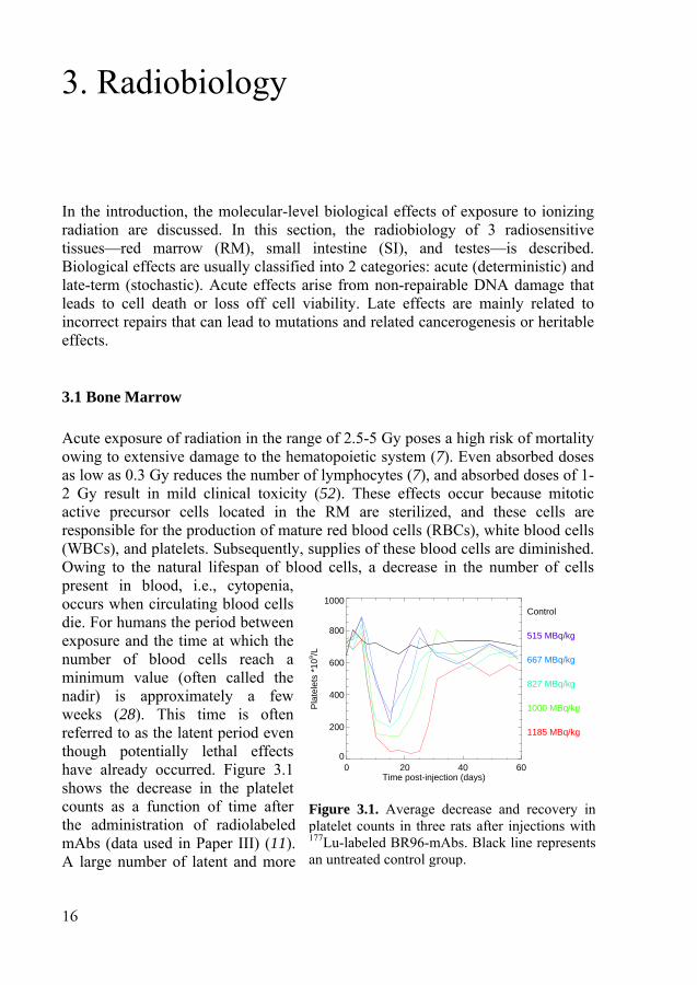
Acute exposure of radiation in the range of 2.5-5 Gy poses a high risk of mortality owing to extensive damage to the hematopoietic system (7). Even absorbed doses as low as 0.3 Gy reduces the number of lymphocytes (7), and absorbed doses of 1-2 Gy result in mild clinical toxicity (52). These effects occur because mitotic active precursor cells located in the RM are sterilized, and these cells are responsible for the production of mature red blood cells (RBCs), white blood cells (WBCs), and platelets. Subsequently, supplies of these blood cells are diminished. Owing to the natural lifespan of blood cells, a decrease in the number of cells present in blood, i.e., cytopenia, occurs when circulating blood cells die. For humans the period between exposure and the time at which the number of blood cells reach a minimum value (often called the nadir) is approximately a few weeks (28). This time is often referred to as the latent period even though potentially lethal effects have already occurred. Figure 3.1 shows the decrease in the platelet counts as a function of time after the administration of radiolabeled mAbs (data used in Paper III) (11). A large number of latent and more

Figure 3.1. Average decrease and recovery inplatelet counts in three rats after injections with177Lu-labeled BR96-mAbs. Black line representsan untreated control group.

0 20 40 60Time post-injection (days)

0

200

400

600

800

1000

Pla

tele

ts *

109 /L

Control

515 MBq/kg

667 MBq/kg

827 MBq/kg

1000 MBq/kg

1185 MBq/kg

17

radioresistant hematopoietic stem cells are in a quiescent phase, G0, and can be activated when needed, so blood cell count may recover after appropriate medical treatment. The 50% lethal doses for acute exposure for various mammals are given in Table 3.1.

The hazardous acute effect of radiation to WBCs is usually granulocyte depression, which can, owing to the suppressed immune system, lead to infection and fever. Individuals who receive these high absorbed doses can therefore be treated with prophylactic antibiotics. Effects from RBC depression (anemia) do not usually occur, mainly owing to the long circulation time (months) of RBCs. Platelet depression can lead to impairment of immune mechanisms and hemorrhage (possible anemia).

Table 3.1. Fifty percent lethal doses (LD50) for various species. (7)

Species Average body

weight [kg] LD50 total-body irradiation

[Gy] Mouse 0.025 7 Rat 0.2 6.75 Rhesus Monkey 2.8 5.25 Dog 12 3.7 Human 70 4

Aside from the dangers from the acute effects, a risk of stochastic effects also occurs after exposure to radiation. Stochastic effects in the BM include an increased risk of leukemia. The latent time between exposure and malignancy is short for leukemia, reaching a maximum after about 5-7 years (7). Conversely, solid tumors often show a latent period of 10-60 years. The risk of developing leukemia has been reported to be linear-quadratic up to 3 Gy (53), with estimated risks of 0.3–0.5% Sv-1 at 0.1 Sv, and 0.6–1.0% Sv-1 at 1 Sv (54).

18

3.2 Small Intestines

Most digestion and related absorption of water and nutrients occurs in the small intestine (SI). Anatomically, the mucous membrane forms cylinder shaped folds, called villi (Figure 3.2). The villi are lined with epithelial cells with protrusions called micro-villi. This shape provides a large surface area of intestinal wall, which maximizes absorption. Owing to the environment in the SI, the cells at the top of the villi are continuously sloughed off at a slow rate and replaced by new cells that originate from mitosis at the base of the villi—the so-called crypt cells. These cells move toward the tip of the villi, where they are eventually lost into the intestinal contents.

An acute total body irradiation of more than 10 Gy leads to the gastrointestinal syndrome within several days (7) and leads to death in most mammals. No essential effect occurs in the differentiated cells on the villi at these absorbed doses, but the crypt cells are undifferentiated stem cells that are radiosensitive (55) and, therefore, sterilized. If the epithelial cells on the villi are not replaced, the tips of the villi continue to slough away, and the villi begin to shrink. Eventually, the inner surface lining is completely denuded of villi. Rodents reach this condition between 3 and 4 days after exposure, and monkeys (and presumably humans) in 5-10 days. Therefore, access to a small-scale dosimetry models that accurately calculate the absorbed dose to the crypt cells is important to be able to predict severe side-effects (Paper IV).

Stochastic effects induced in the SI after radiation exposure are unverified, perhaps because the studies carried out have been based on low-LET radiation at high absorbed doses, which might have resulted in cell sterilization (54).

Figure 3.2. Schematic cross-section of the small intestinal wall (redrawn from Jönsson et al. (12)).

Crypt

MucosaVilli

Serosa

Submucosa

Mucus

Muscularis

Contents Ø 25 mm

19

3.3 Testis

The testis is one of the most radiosensitive organs. Testicular exposure to externally uniform irradiation at sufficiently high absorbed doses leads to deterministic damage that is well understood (56). The threshold for absorbed doses that result in temporary sterility is as low as 0.15 Gy when received in a single high-dose-rate exposure, whereas permanent sterility requires an absorbed dose of 3.5-6.0 Gy. The annual dose rates causing temporary and permanent sterility from highly fractionated or protracted exposure over a period of several years have been specified by the ICRP to be 0.4 Gy y-1 and 2.0 Gy y-1, respectively (57).

The testis is composed of long cylindrical seminiferous tubules that produce spermatozoa through the process spermatogenesis. Another feature of the testis of minor importance in radiobiology is the release of testosterone.

The basement membrane, or lamina propriai, of the seminiferous tubules is made up of 5–7 cellular layers separated by laminae of extracellular connective tissue components. Each tubule is lined with a seminiferous epithelium composed of columnar supporting cells called Sertoli cells and the germ cells of the spermatogenic lineage. Figure 3.3 illustrates the anatomy of the testis used in Paper V. The architectural arrangement of the seminiferous epithelium starts from the basement membrane with the highly radiosensitive germ cells, spermatogonia. These germ cells undergo mitosis and form either type AS spermatogonia stem cells or type AP spermatogonia progenitor cells, the latter dividing several times to form type B spermatogonia. On the inner side of these cells lie the primary spermatocytes, which arise from type B spermatogonia through mitotic cell division. Each primary spermatocyte then produces 2 secondary spermatocytes (pre-spermatids) through maturation division. These cells divide quickly to become haploid spermatids, differentiating into mature sperm cells that are released into the lumen of the tubule. The spermatozoa secreted by the seminiferous tubules are collected in the rete testis and delivered to the excurrent ductal system of the epididymis (58). The transit time from mitosis in spermatogonia to spermatozoa in humans is 74 days.

The radiobiological response of testicular cells undergoing spermatogenesis to ionizing radiation has been well established in the mouse and rat (59-61) and is considered relevant to humans (62). Spermatogonia in the early stage of differentiation are much more sensitive to radiation than cells in the later stages of maturation, i.e., primary and secondary spermatocytes, spermatids, and spermatozoa (63, 64).

20

Figure 3.3. Principal alignment of cells in the seminiferous tubules, in which cell division starts in the spermatogonia and gradually develops toward the lumen to become spermatozoa (adapted from Paper V).

A correlation between occupational ionizing radiation exposure and the development of testicular cancer has not been verified (53). Risks from internal emitters still need to be assessed, as the few studies reported a somewhat increased testicular cancer risk (65). Epidemiologic studies have not provided a clear evidence of excess heritable effects to coming generations owing to mutations in spermatozoa (66).

2. Lamina propria (8 µm)

3. Spermatogonia (9-12 µm)

4. Primary spermatocytes (16-18 µm)

7. Secondary spermatocytes (7-8 µm)

8. Mature spermatids (5 µm)

8 µm

10 µm

15 µm

15 µm

10 µm 1. Interstitial tissue

7.5 µm

7.5 µm

5 µm

9. Lumen30-60 µm

Source/target

6. Secondary spermatocytes (7-8 µm)

5. Primary spermatocytes (16-18 µm)

21

4. Radionuclides

Various radionuclides have been evaluated in the works presented in this thesis (Table 4.1). Some are mainly used for imaging (18F, 67Ga, 99Tcm, and 111In), whereas 90Y, 131I, 177LU and 211At are important for RNT. The visualization of the radial energy distribution from point sources of the different radionuclides are shown in Figure 4.1.

The physical properties (decay data) of the radionuclides used were obtained from the Radiation Decay 3 software (Charles Hacker, Griffith University, Gold Cost, Australia). This program uses radionuclide data compiled by the Radiation Shielding Information Center at Oak Ridge National Laboratories, TN, USA. The data for the energy spectrum of the β-particles were taken from the RADAR website (67).

Radionuclides suitable for RNT must conform to 3 criteria:

1. The half-life must be suitable for the biodistribution of the radiopharmaceutical. A large molecule, like a mAb, displays a slow uptake rate in tumors and normal organs. An optimum physical half-life is on the order of days, whereas radionuclides with shorter half-lives can be used for smaller molecules with faster biokinetics.

2. The energy of the emitted particles should primarily be absorbed within the target tissue to minimize unwanted absorbed doses to healthy organs with related adverse effects. The radionuclide should emit particles with a suitable range for the sizes of the tumors. For radiopharmaceuticals internalized in a cell nucleus, particles with very low kinetic energy can have a large biological effect. The absorbed dose to other cells from these particles is very small, however, implying that if some tumor cells lack uptake, the treatment may be unsuccessful. For long-range β-emitters, the cross-doses to surrounding cells can be significant, which may lead to cell death in cells without activity uptake.

3. If the radionuclide is used in a non-ionic form, its chemical properties should allow for chemical labeling techniques. Halogens and metals are two groups of radionuclides frequently used in RNT. The halogens are connected to the tracer with a carbon bond, whereas metals are labeled with a chelate between the tracer and the radionuclide.

22

Table 4.1. Predominant emissions of radionuclides studied in this thesis. Data from Radiation Shielding Information Center at Oak Ridge National Laboratories, TN, USA. 211At decays with a 58% probability to the short-lived 211Po.

Nuclide Half-life Decay type (average energy, yield) 18F 1.83 h e+ (250 keV, 96.7%) 67Ga 3.26 d e– (0.99 keV, 165%), e– (81-93 keV, 31.4%),

γ (8.6-9.6 keV, 55.4%), γ (91.2-93.3 keV, 38.6%), γ (184 keV, 19.7%), γ (300 keV, 16.0%)

90Y 2.67 d β– (935 keV, 100%) 99Tcm 6.02 h e– (1.6-2.2 keV, 109%), e– (119-122 keV, 9.4%),

γ (18.2-20.2 keV, 7.33%), γ (141 keV, 89.1%) 111In 2.83 d e– (2.7 keV, 100%), e– (145 keV, 8.4%), e– (218 keV, 5.0%),

γ (22-26 keV, 82.8%), γ (171 keV, 90%), γ (245 keV, 94%) 124I 4.18 d β+ (686 keV, 11%), β+ (974 keV, 12%),

γ (27-31 keV, 58%), γ (603 keV, 59%), γ (1691 keV, 10.1%) 125I 60.14 d e– (3.2 keV, 156.1%), e– (22.7-35.3 keV, 35.2%),

γ (27-35 keV, 144.3%), 131I 8.04 d β– (96.6 keV, 7.4%), β− (192 keV, 89.3%), γ (364 keV, 81%)

177Lu 6.61 d β– (47.3 keV, 12.3%), β− (111 keV, 9%), β– (149 keV, 78.7%), γ (113 keV, 6.4%), γ (208 keV, 11.0%)

211At 7.21 h α (5.87 MeV, 41.7%), γ (76-90 keV, 43.5%) 211Po 0.52 s α (7.45 MeV, 98.9%)

23

Figure 4.1. Radial distribution of the energy imparted from a point source in water. The y-axis was optimized for the visualization of the majority of the spectrum. Very low-energy-electrons (<10 keV) add to the deposited energy close to the source, and the maximal value of the deposited energy per bin is displayed numerically in each figure. To evaluate the absorbed dose profile, the energy distribution is divided by the mass (proportional to the square of the distance). For 211At, the 211Po daughter nuclide was included owing to the short half-life of 0.52 seconds.

0.00 0.02 0.04 0.06 0.08 0.10Distance (mm)

0

2

4

6

8

10M

eV/c

m

125IMax 43.2 MeV/cm

0.00 0.02 0.04 0.06 0.08 0.10Distance (mm)

0

500

1000

1500

2000

MeV

/cm

211AtMax 1600 MeV/cm

0.00 0.05 0.10 0.15 0.20Distance (mm)

0

1

2

3

4

5

MeV

/cm

67GaMax 10.5 MeV/cm

0.0 0.1 0.2 0.3 0.4 0.5Distance (mm)

0.0

0.2

0.4

0.6

0.8

1.0

1.2

MeV

/cm

99Tcm

Max 4.91 MeV/cm

0.0 0.2 0.4 0.6 0.8 1.0Distance (mm)

0.0

0.2

0.4

0.6

0.8

1.0

1.2

MeV

/cm

111InMax 9.71 MeV/cm

0 1 2 3Distance (mm)

0

2

4

6

8

MeV

/cm

177LuMax 7.54 MeV/cm

0 1 2 3Distance (mm)

0

1

2

3

4

5

6

MeV

/cm

131IMax 5.22 MeV/cm

0 1 2 3Distance (mm)

0

1

2

3

4

MeV

/cm

18FMax 6.09 MeV/cm

0 2 4 6 8 10Distance (mm)

0.0

0.2

0.4

0.6

MeV

/cm

124IMax 5.93 MeV/cm

0 2 4 6 8 10 12Distance (mm)

0.0

0.5

1.0

1.5

2.0

2.5

MeV

/cm

90YMax 2.16 MeV/cm

24

5. Imaging

Imaging with scintillation cameras, SPECT, or PET is the most common procedure for diagnostic examinations in NM. Imaging is also important for RNT to determine whether the uptake is sufficient to proceed with therapy or to evaluate the effect of a treatment. Quantitative imaging is important for accurate determination of the activity as a function of time for dosimetry calculations. Therefore, applying appropriate correction methods for scatter and attenuation are also important. A standard Anger scintillation camera produces planar images. A common procedure for quantifying activity is to measure a set of anterior-posterior images from which to derive a geometrical-mean image. The attenuation compensation at a point is then based only on patient thickness. A scintillation camera can also be used to acquire images in different projections around the patient. These projections can be used in a reconstruction algorithm to obtain a set of transversal two-dimensional images that form a 3D volume. For small objects, the partial volume effect owing to the limited spatial resolution of the system is a problem that must be considered.

The spatial resolutions of clinical SPECT and PET systems are in the order of 10-15 mm and 5-7 mm, respectively. These orders are, however, too large to quantify the activity concentration in the source regions for the dosimetry models developed in this thesis. Therefore, NM preclinical imaging systems that have considerably better spatial resolution, yet are quantitative, must be considered.

5.1 Small-animal systems

A research field that has grown quickly is the development and evaluation of dedicated small-animal imaging systems. Currently µSPECT systems can have a spatial resolution less than 0.4 mm, µPET systems just above 1 mm spatial resolution (at central field of view), and small-animal µCT about 40 µm. µCT systems dedicated for small samples can have even better resolutions. Also available are µMRI systems with high magnetic field strengths. Systems often are of a combined type, e.g., µSPECT/µCT and µPET/CT.

These new systems can provide valuable information in many research areas, not to mention in the design and evaluation of new pharmaceuticals (68). For RNT and dosimetry, the images from these systems can be used to follow and quantify time-activity distribution during treatment in an individual animal. This feature is

25

enormously beneficial because it reduces the number of animals needed in a study as well as the fluctuations of individual activity uptake. The anatomical information can also be used in dosimetry models, either by adapting the surfaces of a hybrid phantom after the actual anatomy or by using the anatomical information directly in an MC code for the simulation of particle transport.

Some issues occur with these systems that cannot be ignored. Because the voxel sizes are so small compared to those in clinical systems, the noise related to low count rate is much higher, which suggests that a high level of administered activity is required or a longer acquisition time must be used. Increasing the activity seems like a straightforward approach, but it is important to still work with tracer levels of the pharmaceutical to avoid toxicity and/or affected kinetics. The volume that can be injected could also be a limiting factor. With PET, the number of random coincidences increases as a function of the square of the count rate. Because keeping rodents in a fixed position is difficult, the animals need to be anesthetized or restrained in a narrow tube. Certain anesthetizing agents are known to affect the normal kinetics of a tracer (69), whereas keeping the animal restrained causes enormous stress. Modern µSPECT systems are usually equipped with multiple pinhole collimators that produce images with exceptionally high spatial resolution. Because the sensitivity of these collimators is not independent of source location, however, compensation for attenuation is more complicated. Images obtained using µPET have a slightly larger spatial resolution owing to in-flight annihilation, detector design, and the fact that annihilation photons are not created at the decay location. The effect of photon attenuation is lower owing to the 511-keV photon energy, however, and easier to correct for. Outside the central field-of-view, the

depth of interaction in the crystals gives rise to a parallax error that increases the spatial resolution. The absorbed dose from µCT is far from lethal but is reportedly high enough to cause biological effects that can interfere with a dose/response

Figure 5.1. µSPECT (Bioscan NanoSPECT/CT) of a healthy mouse injected intravenouslywith 99Tcm-labeled HER2 (human epidermal growth factor receptor 2) -specific affibody,with activities mainly in the kidneys and bladder. Courtesy of Jonas Ahlstedt, Departmentof Medical Radiation Physics, Lund University.

26

study. In an MC study of a typical µCT screening examination with a reconstruction voxel size of 200 µm (70), the average whole-body dose varied from 80 mGy (at 80 kVp) to 160 mGy (at 50 kVp). In a kinetic study of 5 time points, each with a µCT at 50 kVp, the whole-body absorbed dose is 800 mGy.

5.2 Autoradiography

For tissues in which the activity distribution is often considerably heterogeneous, and needs to be investigated in more detail, we are limited to ex vivo techniques. One technique is autoradiography (ARG), in which thin sections of the tissue are placed in close contact with a detector.

Figure 5.2. Film autoradiography of a 60-µm-thick whole-body section of a rat 5 days post-injection with 111In-oxine. The image shows a heterogeneous uptake with activity in for instance liver, bone marrow, intestinal wall, and testes. Courtesy of Bo-Anders Jönsson, Department of Medical Radiation Physics, Lund University.

Classically, the most used technique is film ARG, which can be applied at a macroscopic level, i.e., whole-body ARG of the biodistribution in sections from animals (Figure 5.2), light microscopic ARG of small tissue sections or even

sinlocmodevtheaboimathetheem

OnARphofilmthedigBioOslsid6.3isospeima

FigcurimadisthistDepRad

ngle calizonocvelope sizove age.

e filme nu

mulsi

n theRG hosphm, he scrgital omelo).

ded s3 × tope

ectraage

gure rativeage tributologpartmdiatio

celation

chromped

ze ofall t The

m—umbon,

e mahas ihor shave reens

recdicaEmi

silico2.6 e ima or is sh

5.3.e acof t

utiongicalmenton P

lls, ns mati“im

f thethe ee im

—or iner oand

acroin mstoraa di

s mucordal Ceittedon-scm2

maginsuf

how

. (Letivitythe s

n in tl sects of

Physi

and(71

ic somage

e silemis

magen theof gdev

oscopmost age igitaultiping. ented parstrip 2. Thng cafficie

wn in

eft) Ty ofsamethe pctionf Oncics, L

d e). Tolid

es” hlver ssions aree cagrain

velop

pic casescre

al reple t

Thr is rticldete

he san bently

n Fig

Tumf 177Le secperipn wicoloLund

electThes

d or have

gran che no

ase ons—ping

levees reeens adouime

he dthe es (tectosystebe acy di

gure

mor sLu-Bction

pheryith ngy, L

d Un

tron se liqu

e a hains haracot dirof lig

—depg equ

el, ieplathat

ut ws. A

digitaBiotypi

or wiem hchieviffer5.3.

sectioBR96n (By of no aLundivers

mtechuid

high and

cterirectlght mpenduipm

.e., ced t, w

with bAnoth

al Amolcallyith ahas ved ent .

on st6 mo

Biomthe

appard Unsity.

icrohniqfilmintr

d theistic ly qumicrd onment

resowhohile betther sARGlex 7y β±

a 50-spatusinhalf

taineonoc

molextumrent niver

oscopques m emrinsice thiand

uantroscon exand

olutiole-bexp

er lisolu

G sy700 ±) are-µmtial,

ng raf-liv

ed wclonax 70

mor aacti

rsity,

pic are

mulsc spicknd tistitatiopicxposd tec

ion bodyposeinearutionystemReae reg

m intr tem

adionves (

with hal an0 Im

and tivity, and

ARe bsion patianess sue ive, c ARsure hniq

abovy AR

ed inrity

n form aal-Tigisterinsi

mpornucl(72).

hemntibomagethe ny uptd An

RG based

witl resof tsamhow

RG atim

que,

ve aRG. n a mand

r quaavailime eredic reral, lides. An

matoxody. er). Nnew takenders

visud oth asolutthe

mple weveand me,

amo

apprMo

mannd offeantitlableDig

d usinesoluand

s witn ex

xylin (RigNotetumo. Cos Örb

ualizon a radtionfilmthic

er, beelecthe

ong

roximost mner

fer thtative at

gital ng autiond eneth ei

xamp

andght)e theor mourtebom

zatiothe dioa

n tham emckneecau

ctronch

othe

matemodesimihe cave At theIma

a 300n anergyitherple

d eosDig

e hemass esy

m, De

on irr

activat is mulsess tuse tn miharacer in

ely 5ern lilar apab

ARG e Luager 0-µm

nd a y resr difof a

sin, 7gital eteroat thof S

epart

of radiave slimiion.

that the bicroscterinflue

50 μlaboto thbilityis t

und (Bio

m-thfieldsolutfferina sin

7 daauto

ogenehe bSophtmen

subationampited Thdegr

blackscopstic ence

μm—oratohat uy ofto us

Unomohick d of tionng engle

ays aoradeous

bottomhie Ent of

bcelln ople. only

hus, radeknes

pic Aof

es.

—digoriesusedf reuse diniverolex dou

f view. M

emis-iso

after diogra

actm ofEriksf Med

27

lularof a

They byit is

e thess ofARG

the

gitals used forusingirectrsityAS,

uble-w of

Multi-ssiontope

sub-aphytivityf thessondical

7

r a e y s e f

G e

l e r g t y , -f -n e

-y y e , l

28

6

In(hmpacanemth

6.

Inphas

Inchmwelus(7Puphpapha 10inOarwhuththw

8

6.

n inthuma

mathearticalculeede

mediuhe m

.1 H

nternhants sph

n theharac

mathewith llipsosed p73, 7ublichantarallhantrang

0, annto tLIN

rguawere

umahe lahe st

well

Ph

ternaan, nematcle tlatioed inum o

most c

Huma

nal dtomshere

e 19cteriematsimoidsphan

74). catiotomslel wtomsge ond 1the

NDAably

maan poate etrengdefi

ha

al ranewticaltranson ofn all or a com

an w

doses uses an

960sistictical

mple s, plntomTheon 2s beworks (21of sim15 yeMIR

A/EXdo n

ainlyopuleffecgths fined

ant

adiowborn

lly dsporf abspartone

mmon

who

e caled to

nd el

s thecs) l exp

shalanesm wa org23: cam

k res1). LmilaearsRDO

XM not v

y delatiocts oof b

d. T

tom

onucn, mdescrrt ansorbticlee-dimn rep

le-b

lculao calipso

e firwe

presapess, anas de

gan sRef

me knsulteLaterar phs, anOSE(46)visu

eveloon toof iobein

The

m

clidemous

ribednd sbed de tranmenpres

body

ationlculoids

rst aere sion sund tevelshapferennow

ed inr, Crhant

nd ad 3.1). T

uallyopedo be oniz

ng sipha

ms

doe, rad. Tscordosenspo

nsionsenta

y ph

ns wate a

s to d

anthrde

ns ofch tori. lopepes ance

wn an theristytomsdult,1 soThesey repd to

usezing implantom

simeat, et

Thesere ene disort snal ration

anto

wereabsoderiv

ropoevelof theas cOf

d byand m

Mas the ICy ans for, whoftwae so

prese rep

ed inrad

le, flms

etry,tc.) e phnergtribuimurepren is a

oms

e perorbeve an

omoropede orgcomthe

y Snmasan (

he MRP d Ecr thehich are o-caent tpresn risiatiolexibare

, a in w

hantogy dution

ulatioesena 3D

rformd donaly

rphicd. gans

mbinase, t

nydeses w(75)

MIRDPubckere agewer(44

alled the hent k es

on. Tble,

als

phanwhichoms depon. Tons. ntatioD ph

medoses ytica

c phThe

s by ationthe r anwere). ED phblicarmanes ore la) an

styhuman

stimThe ando w

ntomh orcan

ositioThus,

Thion (

hanto

d as wer

al ex

hantey exp

ns omos

nd Fie ba

Eventhant

ationn (76of neater nd iylize

man aave

ationpha

d mawide

m isrgann be on f, a reis repchor

om r

earlre ba

xpres

tomsrel

pressof cst coisher

ased tualltomsn 30 6) dewboincoits sed panatoeragens rantoathemly u

s a n size

usedfromeprepresrd-brefle

ly aasedssion

s (hulied sing cylinommr in on Ily, s (19seri

develorn, orposuccephanomye ofrelateoms matiused

repres, sd in

m eaesentsentabasedectin

s thd on ns o

umao

themndermonl

196ICRthes9). Aies olope1, 5

rateesso

ntomy, buf thed thav

icallyd fo

resenshapan M

ach tatioationd tra

ng th

he 19sim

f AF

an on m s, ly 69 RP se A of ed 5, d

or ms ut he o

ve y

or

FfNpNpcld

ntatipes, aMC par

on ofn canansphe an

940smple Fs.

FigufromN-paplotteNatiophancolorlight-dark-

ion and cod

rticlef then be

port)natom

s, wgeo

re m thearticler ofonal

ntomr rep-grey-grey

of aloca

de toe foe geoe an , bumy.

whenomet

6.1.e Moef the

(7presy ly sof

an oation sim

or fuomeinfin

ut in

n thetries

A onte

geOakLabo

76). ents lungft tiss

objecns ar

mulaturtheetry nitivNM

e firs suc

vi Caome

k Ridorato

Blabon

, asue.

ct re te er is

ve M,

st ch

ew arlo etry dge ory ack ne, and

29

dosimetry calculations in RNT, where a more patient-specific geometrical representation is desired.

As computers have increased in speed and memory, the interest in using the voxel information obtained from CT images to represent the geometry has also increased. Modern hybrid SPECT/CT systems allow the use of CT images of a patient as a computer phantom and the SPECT images as the source of activity. This application is, however, not as a straightforward as it sounds. CT image values are measured in units of Hounsfield that can be converted into an electron density (77) for various tissues (lung, soft tissue, bone). The large effort required is the segmentation of each organ for each of the slices that, if made manually, is extraordinarily time-consuming. A properly segmented phantom, however, represents the geometry of the patient. The downside of this voxel-based phantom is that it is mostly inflexible. The representation is valid only for the patient for which it was developed and only at the time when the CT was performed. If the aim is to derive dosimetry on a voxel level, then the images in a time series must be registered to one another so that they contain information from the same anatomic location in the same voxel location for all images. An interesting feature of working with voxel-based phantoms instead of mathematical phantoms is the difference in the surface area of the organs. For example, the surface of a circle with a diameter represented by voxels has an area equal to (as a cube), “independent” of the voxel resolution. This relationship may be an important consideration when working with low-energy electrons emitted near surfaces because of a partial volume effect (78, 79), or when simulating a flux over a surface.

One of the first available voxel-based phantoms was the Zubal phantom (80). Another voxel phantom is the ADELAIDE Teenage Female Voxel Computational Phantom (81). The GSF voxel phantom family (82) contains of 12 phantoms derived from CT or MRI images. One of these phantoms was obtained from postmortem images of 8-week-old child and another from images of a 7-year-old child with leukemia. The other phantoms represent adults of both genders of various sizes, and the phantom “Katja” represents a pregnant woman in the 24th week. The MAX06 and FAX06 (83) are voxel phantoms based on CT images, anatomical handbooks, and the Atlas of the Visual Human Male (84). These phantoms have been prepared for skeletal dosimetry by segmenting the cortical bone, spongiosa, and yellow marrow. They have also been coupled with µCT images of trabecular bone for MC simulations for RM dosimetry (85). New reference phantoms based on the voxel phantoms “Laura” and “Golem” of the GSF-family adjusted to the reference values in ICRP Publication 89 (86) were described in ICRP Publication 110 (87).

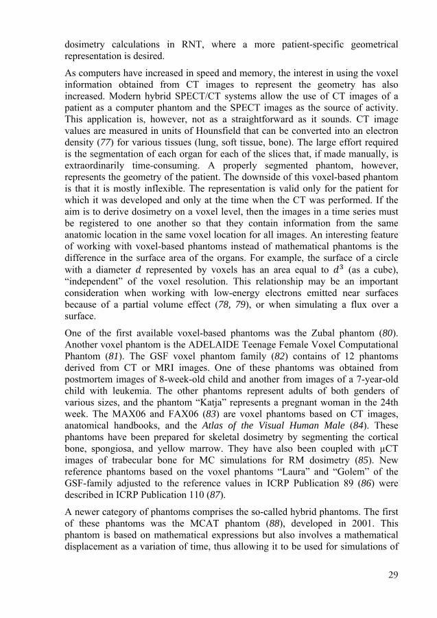
A newer category of phantoms comprises the so-called hybrid phantoms. The first of these phantoms was the MCAT phantom (88), developed in 2001. This phantom is based on mathematical expressions but also involves a mathematical displacement as a variation of time, thus allowing it to be used for simulations of

30

respiratory and heart movements. A commonly used hybrid phantom is the human 4D NCAT developed by Segars et al. (89). Instead of being described by ordinary surfaces, the underlying organ shapes consist of non-uniform rational B-spline (NURBS), a surface type widely used in computer graphics that is based on control points. The phantom is actually software that produces images with characteristics that can be controlled with an input file. The software generates 2 sets of 3D images, one representing the activity per voxel (as specified in the input file), and the other representing the average attenuation within each voxel (depending on the energy specified). The software also contains data that allow for the simulation of physiological movements, such as respiration and cardiac motion, and can thus generate several sets of 3D images as function of time. By translating the control points connected to the NURBS surfaces, the shape and sizes of organs can be modified to match an individual patient or generate a patient population. The 3D images can also be generated at any spatial resolution without introducing errors that otherwise might result from linear interpolation. The adaption of the NURBS was made on 1 specific region at a time using the commercially available software RHINOCEROS® (www.rhino3d.com). Later, Segars et al. developed the mouse and rat whole-body phantoms MOBY (90) and ROBY (91), which have been used extensively in this thesis, and the extended human XCAT phantom (92) (Figure 6.2). To date, no general MC code can handle NURBS surfaces, so for the purpose of particle simulation the phantom has to be voxelized.

Another phantom software based on NURBS is the 4D VIP-Man (93), focused primarily on an accurate segmenting of the RM. The mucosa in the stomach and the upper and lower large intestine is also modeled using thin layers of 0.33 mm and 0.67 mm, respectively.

Researchers at the University of Florida have developed a series of pediatric and adult phantoms (94, 95) based on the NURBS technique. A group at Vanderbilt University is developing its own adult and pediatric NURBS-based phantom series that will be available in the next version of the OLINDA/EXM computer code (96).

A group at Rensselaer Polytechnic Institute (RPI) reported some disadvantages when representing very small objects as NURBS surfaces (97). For the representation of a thin object, such as the trachea, they proposed the use of a polygonal mesh (PM). They constructed the RPI-P3, RPI-P6, and RPI-P9 phantoms of a woman 3, 6, and 9 months pregnant. The more complex surfaces were modeled with PM and the more uniform with NURBS. Their next phantoms, RPI-AM and RPI-FM (98), which represent an adult male and female, were based entirely on PM. In the transport of radiation, the phantoms were still voxelized. Other PM phantoms are the FASH and MASH phantoms (99, 100), which have been developed from the FAX06 and MAX06 phantoms.

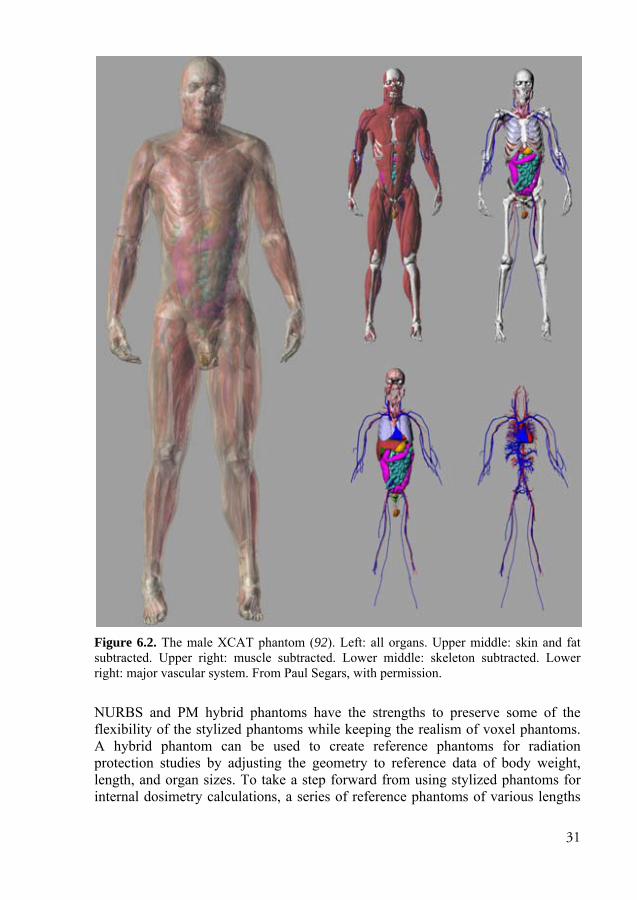
31

Figure 6.2. The male XCAT phantom (92). Left: all organs. Upper middle: skin and fat subtracted. Upper right: muscle subtracted. Lower middle: skeleton subtracted. Lower right: major vascular system. From Paul Segars, with permission.

NURBS and PM hybrid phantoms have the strengths to preserve some of the flexibility of the stylized phantoms while keeping the realism of voxel phantoms. A hybrid phantom can be used to create reference phantoms for radiation protection studies by adjusting the geometry to reference data of body weight, length, and organ sizes. To take a step forward from using stylized phantoms for internal dosimetry calculations, a series of reference phantoms of various lengths

32

and body weights can be derived to calculate S factors. The S factors assigned to patients can then be chosen by selecting the phantom that most closely matches their height and weight. Another step would be to adjust this phantom for body contour; however, the S factors would then have to be simulated using an MC code. For patient-specific dosimetry, the segmentation of the organs is still required to obtain the correct inner anatomy.

Kim et al. (101) have presented a polygon-surface reference Korean male phantom that was directly implemented in the GEANT4 MC code without being voxelized. The simulation times were reported to be 70-150 times slower for photons than for the corresponding voxel phantom, but this increase in CPU time may be acceptable for applications in which accuracy is needed, such as for very thin objects in which voxelization creates a rough structure or 4D dosimetry (movements). The group is now developing methods to improve the simulation time and have to date done so by more than 30 times the reported simulation times.

6.2 Small-animal phantoms

Small-animal dosimetry is essential for evaluating the efficacy of preclinical RNT. Small-scale animal phantoms for mouse and rat were used in Papers I-III. As mentioned in Chapter 2, a phantom representing the proper anatomy is vital for achieving high accuracy in absorbed dose calculations. In small animals like mice and rats, the ranges of emitted electrons and β-particles are often long and therefore, disregarding electron transport to other tissues (cross-dose) is unjustified. Cross-doses from photons are, however, mostly be negligible for photons with energies higher than 40 keV.

Several mathematical phantom models for mouse dosimetry have been presented in the literature. In 1994, Hui et al. (102) presented a geometrical mouse model based mainly on ellipsoids developed from 10 athymic mice weighing approximately 25 g. Muthuswamy et al. (103) extended this model by including BM compartments. Yoriyaz et al. (104) described a geometrical model for a 30-g mouse in 1997. The model presented in 2001 by Flynn et al. (105) was based on ellipsoids and cylinders but included a more realistic model of the kidneys separated into the cortex and medulla, and a spherical tumor separated into a vascular rim and a necrotic core. Hindorf et al. (106) have also developed a voxel-based mouse phantom (24 g) based on combinations of cylinders and ellipsoids, used to investigate the influence of organ anatomy and location on the calculation of the absorbed dose. Kolbert et al. (107) have developed a more anatomically realistic voxel-based model derived from MRI in which the left and right kidneys, liver, and spleen were segmented. In 2006, Stabin et al. (108) developed a realistic voxel-based model of a 27-g mouse in which 10 organs were segmented from µCT images.

33

In many preclinical RNT studies, tumors are inoculated subcutaneously. Bitar et al. (109, 110) have presented a detailed voxel-based model based on a female athymic nude mouse weighing approximately 30 g in which a 100-mg tumor was induced on the right flank. When the tumor contains a significant amount of a radiopharmaceutical, the energy emitted from the tumor can add to the absorbed dose in adjacent organs owing to their proximity.

Several of the mouse models described above were developed from CT or MRI studies of animals, and the geometry is represented by voxels in 3D. Often, each voxel value is coded to represent a particular organ or structure. Although these models can be quite accurate, they still represent an individual specimen, and the possibility of modifying the internal structures in terms of organ size and location is limited. The MOBY phantom, developed by Segars et al. (90), is a hybrid phantom similar to the NCAT/XCAT phantoms. The MOBY phantom was originally developed for the evaluation and optimization of small-animal imaging but was shown to be useful for preclinical dosimetry studies as well (Paper I). This realistic phantom is based on NURBS, and the geometry was developed from a segmented C57BL/6 mouse weighing 33 g. The surfaces allow for flexibility in the shapes of the organs, allowing heart and respiratory motions to be modeled. Thirty-six regions (including 8 heart, 7 brain, and 3 skeletal regions) are segmented. The phantom is software controlled by a user-modified parameter file and generates 2 sets of 3D voxel-based images with the specified matrix size of the activity and the attenuation in the mouse, which then serves as input for MC dosimetry calculations. This phantom was used in Paper I to calculate S factors using the MC code MCNPX. In Paper II, the same phantom was used to investigate the absorbed dose to and from subcutaneous tumors. Keenan et al. (91) have also determined S factors based on the MOBY phantom for mice weighing 25 g, 30 g, and 35 g.

Published dosimetry models for rats are rare, and only a few appear in the literature. Hindorf et al. (111) developed a mathematical model consisting of a combination of ellipsoids and cylinders with volumes based on the average organ masses of 10 Brown Norway rats. Konijnenberg et al. (112) have developed a similar stylized model that represents Wistar rats. Stabin et al. (108) have presented a voxel-based phantom of a 248-g Sprague-Dawley rat that was derived

Figure 6.3. The MOBYphantom. Printed withpermission from PaulSegars.

34

through segmentation of multiple µCT images. Keenan et al. (91) presented the ROBY phantom, developed from a 330-g Wistar rat. Keenan et al. have also calculated S factors for several nuclides and body weights. In Paper III, the ROBY phantom was adapted to the geometry of a BN rat based on average organ weights. This modification was voxelized and served as input for MC simulation of S factors for dosimetry calculations.

Figure 6.4. The voxelized Brown Norwegian version of the ROBY phantom was used in Paper III. The red voxels correspond to red bone marrow compartments, and the blue voxels match a subcutaneous tumor on the flank.

6.3 Small-scale tissue dosimetry models

6.3.1 Small intestine

The radiosensitive crypt cells in the SI wall are important targets for absorbed dose calculations. In Paper IV, a model of the intestinal mucosa based on the work of Jönsson et al. (12) was presented.

The radiosensitive crypt cells are located at the bottom of the villi. Instead of calculating the absorbed dose to the entire SI wall, the absorbed doses are calculated to the crypt cells.

SI content was modeled as a cylinder with a diameter of 25 mm, and the SI wall was modeled as a cylindrical shell of 3 and 6 mm surrounding the contents (Figure 6.5). The orientations of the SI loops are almost randomly distributed within a body. This complex geometry was approximated by modeling the SI in a hexagonal, close-pack geometry.

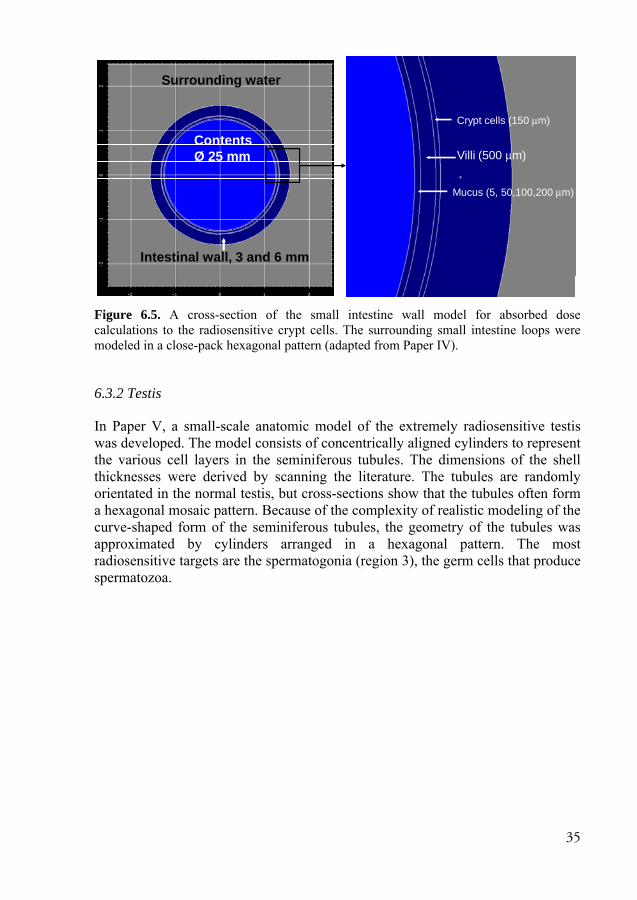
35

Figure 6.5. A cross-section of the small intestine wall model for absorbed dose calculations to the radiosensitive crypt cells. The surrounding small intestine loops were modeled in a close-pack hexagonal pattern (adapted from Paper IV).

6.3.2 Testis

In Paper V, a small-scale anatomic model of the extremely radiosensitive testis was developed. The model consists of concentrically aligned cylinders to represent the various cell layers in the seminiferous tubules. The dimensions of the shell thicknesses were derived by scanning the literature. The tubules are randomly orientated in the normal testis, but cross-sections show that the tubules often form a hexagonal mosaic pattern. Because of the complexity of realistic modeling of the curve-shaped form of the seminiferous tubules, the geometry of the tubules was approximated by cylinders arranged in a hexagonal pattern. The most radiosensitive targets are the spermatogonia (region 3), the germ cells that produce spermatozoa.

Crypt cells (150 μm)

Villi (500 μm)

Mucus (5, 50,100,200 μm)

ContentsØ 25 mm

Surrounding water

Intestinal wall, 3 and 6 mm

36

Figure 6.6. Cross-section of the testis dosimetry model. The seminiferous tubule is modeled as concentric cylinders (regions 2-8), in which the most radiosensitive cells are the spermatogonia in region 3. Between the seminiferous tubules is the interstitial tissue (region 1).

A B

61 23 4 5 78 9

37

7. The Monte Carlo method

7.1 Introduction

Computerized MC techniques first developed when scientists at the Los Alamos Laboratory in New Mexico (USA) were actively pursuing the potential use of computers for multiple statistical calculations of neutron interactions to develop the atomic bomb during World War II. The initial formulation of the MC technique was already being performed in the late 1940s, but the technique evolved along with improvements in computers and programming languages.

The MC technique is useful for solving physical processes in which analytical approaches are not applicable. In short, the MC method applies the theory that physical processes can be described by probability density functions (pdfs) that, if modeled accurately, can be used with pseudo random numbers to sample physical processes directly from the pdf. A large number of histories must be simulated to achieve an estimate of the desired parameter that converges toward an accurate solution. The accuracy of the estimate depends directly on the accuracy of the pdfs, the performance of the actual modeling of the problem, and the quality of the random number sequence and its uniformity.

In NM, MC methods have mainly been used to study the transport of emitted ionizing radiation, either to evaluate imaging techniques or for dosimetry purposes. In addition to simulating ionizing radiation, the propagation of scintillation light in a detector could also be modeled. The pdfs used to model and select possible physical processes are based on cross-section data. Random numbers are also used to sample the location, energy, and emission direction of the particles.

An important and useful feature of MC simulations is the possibly of studying parameters that cannot be measured experimentally. For example, to study imaging quality for quantification purposes, the separation of events coming from photons scattered in the phantom and those that escape from the phantom without scattering is useful to optimize compensation methods. Another example is the study of the effects of photons that penetrate septa walls in the collimator. In the work described in this thesis, the MC method was used for dosimetry calculations in which the energy depositions caused by interacting photons and charged particles emitted from a radioactive source were calculated and tallied (scored) in various target regions.

38

7.2 Photon transport

Photons interact in 4 main ways with related cross-sections: photoelectric effect ( ), coherent scattering ( ), incoherent (Compton) scattering ( ) , and pair production ( ). The total linear attenuation coefficient is given by the following: = + + + Eq. 7.1

These cross-sections depend on the composition of the material and the photon energy. The probability of a photon interacting in a homogeneous medium is given as follows: ( ) = · Eq. 7.2

The probability ( ) that a photon will interact within the distance is given by the following:

( ) = ( ) = 1 − Eq. 7.3

By substituting ( ) with a uniform random number between 0,1], the path length of the photon can be sampled. A random number is as equally randomly distributed as (1 − ), so the path length can be sampled according to equation 7.4. = −1 (1 − ) = −1 ( ) Eq. 7.4

To determine which of the 4 interaction types should be sampled, a new random number is generated. If is in the range 0, / ] , the process is a photoelectric effect. If is in the range ] / , ( + )/ ] , it is a coherent scattering, and so on according to equation 7.5.

=0, ⇒ Photoelectric effect, + ⇒ Coherentscattering+ , + + ⇒ Comptonscattering+ + , 1 ⇒ Pair production

Eq. 7.5

39

If the MC code handles coupled photon-electron transport, any produced electron or positron is stored in memory for later transport. In the case of photoelectric effect, in which the photon is absorbed by the nucleus, the emission of X-rays or Auger electrons may occur, which can be simulated considering florescence yield and atomic relaxation. For coherent scattering, which scatters the photon without losing any energy, the scattering angle is sampled using Thomson cross-sections. In the case of a Compton scattered photon, which scatters the photon with an orbital electron, the energy of the scattered photon is sampled based on the differential Klein-Nishina formula (113), often using Kahn’s method (114). The new direction of the scattered photon can be calculated from the polar angle directly obtained from the energy of the scattered photon and the azimuthal angle, which is sampled isotropically between 0 and 2π.

The Klein-Nishina cross-section is derived from the assumption of a free electron at rest. In reality, electrons are bound to the nucleus to various degrees. Corrections to the Klein-Nishina cross-section to account for the effect of binding can be made using so-called form factors. Atomic electrons also have momentum that can increase or decrease the energy of a scattered photon. This effect is called Doppler energy broadening, which can be modeled using Hartree-Fock Compton profiles (115). For energies above 1022 keV, pair production is possible, where the photon can interact with the nucleus and create an electron-positron pair emitted with a total kinetic energy of hν - 1022 keV shared between the 2 particles. A fundamental difference exists in how a photon MC program and a coupled photon-electron MC code handle the annihilation process. In the photon code, it is uncommon to sample the positron range to the point of annihilation where two 511-keV photons are emitted in opposite directions. Another feature that is usually approximated in a photon code is the treatment of bremsstrahlung photons, which can be produced during electron interactions along the electron path. In the photon code, the bremsstrahlung production is either completely omitted or a thick target approximation is used, where bremsstrahlung is produced at the point where the electron trajectory would have started—i.e., the point of decay or a photon interaction point at which a secondary electron is produced.

7.3 Electron transport

The simulation of electrons is fundamentally different from uncharged particles such as neutrons and photons that undergo few interactions with a relatively long mean-free path length compared to electrons that are affected by Coulomb forces that result in many interactions with matter. The vast majority of electron interactions are so-called inelastic scattering with atomic electrons, resulting in low energy loss and small angular deflection per interaction. Other more rare interactions (catastrophic events) include elastic scattering with the atomic nuclei,

40

the production of secondary knock-on electrons, bremsstrahlung production and, if possible, nuclear interactions. To simulate a single 0.5-MeV electron in aluminum would roughly mean 105 interactions with small-angle scattering. To reduce the calculation time to practical levels, many MC codes have adopted methods that replace many electron interactions with larger steps—a method proposed by Berger in 1963 called multiple scattering or condensed histories (116). Berger proposed 2 simulation strategies, class I and class II electron transport, in his 1963 work:

Class I (complete grouping). This simpler strategy of the 2 classes relies on sets of predetermined path lengths (or predetermined energy losses). Class I includes the effects of both elastic and inelastic interactions along a path length and is described using approximate multiple-scattering theories.

Class II (mixed schemes). Inelastic interactions are simulated individually from the associated differential cross-sections, and elastic interactions are described collectively using fairly accurate multiple-scattering approaches.

The energy loss and angular deflection of electrons during each of the steps can be sampled from probability distributions based on the appropriate multiple-scattering theory. Nearly all current MC codes that adapt multiple-scattering methods for electrons are based on the Goudsmit-Saunderson theory (117) for the sampling of angular deflection. The solution of this theory is an exact expression of the angular distribution after n interactions. This theory does not include the energy loss, however. The sampling of energy loss (or step length) can be performed by the continuous slowing down approximation, but a more accurate theory that considers the statistical fluctuation of energy loss was described by Landau (118). This theory excludes the spatial deflection resulting from the multiple scattering of an electron, which is included in the Lewis theory (119).

Some MC codes work in detailed mode (i.e., simulating each interaction in an explicit mode). The Penelope MC program has a class II electron transport and the ability to switch to a detailed simulation when the scattering angle is large, i.e., a catastrophic event has occurred.

7.4 Variance reduction

Variance reduction is a generic term for methods that improve the statistics of the simulation for a fixed computing time. One of the simpler variance reduction methods is the use of an energy cut-off. If the energy of a particle is lower than a predefined value, it is regarded as unimportant and the history is terminated. The use of a cut-off is not a classical variance reduction technique in the sense that the simulated particles add more information, but because the histories terminate earlier, more histories can be run in the same amount of time. Several variance

41

reduction techniques can be used in an MC code, 2 of which are described as examples below.

One widely used variance reduction technique is particle splitting in combination with “Russian roulette.” In geometric regions of more importance, or if some trajectories are more favorable, particles can be split into multiple daughter particles each assigned a weight = / . Each particle is tracked separately and the scored result in the tally (detector) is finally multiplied by the particle weight. When exiting such a region, Russian roulette is played. A random number R is compared to the difference in importances between the regions and determines whether the particles is terminated or continues with a new weight. This variance reduction thus increases the simulation time per history but if used properly, decreases the variance of the estimate.

Forced detection is a useful variance reduction technique for particles that transverse through a tally region with a low probability of interaction. The particles can then be forced to interact within the tally, and the tally results are multiplied with an appropriate weight.

7.5 General Monte Carlo codes

In addition to the MCNP codes that have been used in this work and are described in detail in the next section, several other general MC codes are useful for dosimetry calculations: The EGSnrc (120) (electron gamma shower) is a coupled electron-photon code with an electron transport based on the Goudsmit-Saunderson theory. It includes the sophisticated PRESTA II algorithm that switches from multiple scattering to single scattering when electrons are close to boundaries (beneath a “skin-depth”), thereby eliminating step-size artifacts due to boundary crossings. The MC code Penelope (121, 122) is an electron-photon code with a class II electron algorithm that uses multiple scattering if the scattering angle is less than a specified value. Otherwise, it switches to single scattering, i.e., for catastrophic events. By setting the value of the angle to zero, the code thereby actually simulates the electrons in a single scattering way. The GEANT4 (123, 124) is a toolkit for photon-electron transport and a wide range of other charged particles. The GATE open source interface (125), built around the GEANT4 physics engine, has been developed with focus on the simulation of PET, SPECT, and CT systems and radiotherapy experiments.

The MCNP codes (126, 127) used in this thesis were chosen because they could be used for simulations of electrons, photons, and alpha particles without major programming requirements. The electron transport calculations in the MCNP codes do not include the state-of-art methods, but by knowing the limitations and how to set up the parameters related to the simulation of the interactions, we believe that the absence of these methods was not a limiting factor for our research

42

objectives. The difference between the new electron sampling implemented in the later versions of the MCNP5 code and the sampling in the others is small in terms of accuracy for our applications.

7.6 The MCNP5/MCNPX code package

The MCNP code has a history that reaches back to the 1960s when the first version of the code was written in FORTRAN at Los Alamos Laboratory. At that point the code was used mainly for 3D simulations of neutron transport. Gamma transport was added during the 1970s, at which point the code was called MCNG (Monte Carlo Neutron Gamma). This addition was followed shortly thereafter by a generalization to perform photon transport calculations as well as criticality calculations. The code was renamed to “MCNP” (Monte Carlo Neutron Photon. During the 1980s the MCNP code was updated with tally plotting and generalization of source specification. In the 1990s, the MCNP4 (now Monte Carlo N-Particle) code was released, and this version increased the flexibility and use of the code through the implementation of the Integrated TIGER Series (ITS) (128) Monte Carlo system for electron transport calculations. MCNP5, launched in 2002, includes small enhancements, e.g., new cross-sections for photons, improved functionality of the geometry specification, and a visual editor.

A parallel development on the MCNPX code package was initiated in the mid-1990s. This code was built on MCNP4B, with its neutron-photon-electron transport capabilities, and the Los Alamos High-Energy Transport code built for high-energy particle transport calculations. The MCNPX code now includes the standard geometry and physics modules—albeit not always the latest versions—with an extended use allowing for transport calculations for α-particles, muons, ~2200 light, and heavy ions, among others.

The MCNP code is controlled with input files that contain blocks. The first block consists of lines, or cards (originating from the time when punch cards were used) that describe the surfaces used to build the geometry. This block is followed by a block of lines that defines different segments of the geometry, called cells. Each cell is linked to a material number, a density, and a structure, which state which surfaces and their related combinations that define the region. Furthermore, material cards specify the atomic compositions and which cross-section tables to use. Also included are physics cards that control the physics, and source cards to specify the source geometry, particle type, energy, direction, and other characteristics. The tally cards are like detectors that are placed at points of interest to score the data to be calculated.

43

7.6.1 Photons

The MCNP contains an option that selects either photon transport only with electron transport turned off (Mode P) or a mode with coupled photon/electron transport (Mode PE). The photon physics models in these 2 modes are similar, the only difference being in the generation of bremsstrahlung and annihilation photons created from secondary electrons and positrons. Two options are available for Mode P. The default option includes a thick-target bremsstrahlung model, in which electrons and positrons are produced but immediately slowed to rest so that bremsstrahlung and annihilation photons are generated directly at the interaction point of the photon. The second option omits bremsstrahlung photons completely but includes the annihilation photons. In Mode PE, secondary electrons and positrons are stored for later transport and can then produce bremsstrahlung photons along their trajectories and annihilation photons at the end of the positron track. The advantage in running Mode P is that time-consuming electron transport is avoided and thereby the simulation time (or variance) is greatly reduced.

The most recent photon cross-section data are processed from the ENDF/B-VI.8 library and include incoherent, coherent, photoelectric effect, and pair production cross-sections for energies from 1 keV to 100 GeV and for atomic numbers Z between 1 and 100. In the case of a photoelectric effect, data of photo-atomic and atomic relaxation are extracted from the EPDL97 library (129). Also included are coherent form factors, incoherent scattering functions, fluorescence data (130), and the bound electron momentum (115). These bonded electrons can add or subtract energy to an incoherent scattered photon resulting in Doppler energy broadening of the scattered photon. The differential Klein-Nishina cross-sections are sampled using Kahn’s method (114) below 1.5 MeV and Koblinger’s method (131) above 1.5 MeV.

7.6.2 Electrons To allow for realistic long simulation times, MCNP uses a multiple-scattering method (116) for electrons, as described previous, in which many small electron interactions are condensed into larger steps. MCNP is built around the ITS 3.0 code (132), which in turn is based on the ETRAN code (128). It is defined as a class I electron transport code and has until recently only used pre-calculated energy steps (new option described below). Alternative energy loss straggling methods can be selected.

MCNP uses a class I algorithm for collisional energy loss and a class II algorithm for radiative losses. The Goudsmit-Saunderson (117) theory is used to calculate angular deflections and the energy loss fluctuations (step length) are calculated using the Landau theory (118) with Blunck and Leisegang (133) enhancements for the binding effects of the atomic electrons. These models require that the energy

44

loss is small compared to the electron energy. Therefore major steps with predetermined step lengths are chosen so that the average energy loss is 8.3%. = 2 / ≈ 91.7% Eq. 7.6

The Landau-Blunk-Leisegang theory for energy loss is applied once per major step. The Goudsmit-Saunderson theory is valid for arbitrary angular deflections, but the electron trajectory is more accurately represented if the major energy steps are divided into a number of substeps , all with the step length / . For geometries that are large compared to , the default value of m probably requires no tempering. For smaller geometries, however, the number of substeps could influence the accuracy of the electron trajectory. It is recommended that an electron undergo at least 10 substeps in a cell before leaving. Raising the number of substeps, of course, also increases the simulation time.

During MCNP initialization, step lengths and parameters for energy loss are pre-calculated in discrete energies on an energy grid , , … , , , . A low value of corresponds to a higher energy, and is equal to the maximum energy specified in the input file. Owing to the fluctuation of the energy loss after a completed major step or in the case of bremsstrahlung production, a rather subtle logic (called the energy indexing algorithm) has been developed to determine which cross-section data to assign to the next major step (Eq 7.7).

MCNP style: > ≥

ITS style: ( + )/2 > ≥ ( + )/2 Eq. 7.7

The default algorithm is the MCNP style, also called bin centered. An electron with energy > > is said to be in group n, and this algorithm assigns the transport parameters calculated for the upper boundary ( ) of the group throughout the whole energy step. Another option is the so-called ITS-style indexing algorithm. This method assigns the transport parameters from the group with the upper boundary closest to the electron energy (nearest boundary). The difference between the 2 logics causes the MCNP-style energy indexing algorithm to assign electron cross-section data, which are, on average, half a group higher than those in the ITS-style algorithm, introducing a systematic error in the MCNP logic. The ITS logic is the most accurate of the 2 logics (134), but for historical reasons, the MCNP logic remains the default. The systematic error can be seen for the large shell size in Figure 7.1, in which the electron range is longer for the MCNP logic than for the ITS logic owing to the assignment of transport parameters at higher energies.

The ITS method has some limitations regarding the accuracy. When an electron crosses a surface, the energy step is interrupted and the particle will not lose the sampled energy loss and then relies on a linear interpolation of a nonlinear theory.

45

If there are many surfaces for the electron to cross, the energy loss can be affected and, in turn, the angular deflection and range.

Introduced in MCNP 5 1.40 is a new logic for electron transport that does not rely on a pre-calculated energy grid but instead calculates transport parameters at every substep. This method is much more robust and allows for a more precise simulation in small cells, as exemplified in Figure 7.1. For 2-MeV mono-energetic electrons, essentially the maximum energy in RNT, the old methods diverges at shell thicknesses of about 250 µm, whereas the new logic works at thicknesses as small as 5 µm. The drawback is that this new algorithm is much more time consuming than the previous 2 algorithms.

Figure 7.1. Energy deposition from a 2-MeV point source in water to varying spherical layers from 1-µm thickness to 1-mm thickness. The upper row shows the Monte Carlo N-Particle (MCNP) energy indexing logic for 3, 10, and 100 substeps. The middle row shows the same data, but for the Integrated TIGER Series logic. The lower row shows the improved logic introduced in MCNP5 1.4.

0 2 4 6 8 10 12Distance (mm)

0

1

2

3

4

MeV

/cm

1

MCNP logicSubsteps = 3

5

MCNP logicSubsteps = 3

10

MCNP logicSubsteps = 3

100

MCNP logicSubsteps = 3

250

MCNP logicSubsteps = 3

1000

MCNP logicSubsteps = 3

0 2 4 6 8 10 12Distance (mm)

0

1

2

3

4M

eV/c

m

1

MCNP logicSubsteps = 10

5

MCNP logicSubsteps = 10

10

MCNP logicSubsteps = 10

100

MCNP logicSubsteps = 10

250

MCNP logicSubsteps = 10

1000

MCNP logicSubsteps = 10

0 2 4 6 8 10 12Distance (mm)

0

1

2

3

4

MeV

/cm

1

MCNP logicSubsteps = 100

5

MCNP logicSubsteps = 100

10

MCNP logicSubsteps = 100

100

MCNP logicSubsteps = 100

250

MCNP logicSubsteps = 100

1000

MCNP logicSubsteps = 100

0 2 4 6 8 10 12Distance (mm)

0

1

2

3

4

MeV

/cm

1

ITS logicSubsteps = 3

5

ITS logicSubsteps = 3

10

ITS logicSubsteps = 3

100

ITS logicSubsteps = 3

250

ITS logicSubsteps = 3

1000

ITS logicSubsteps = 3

0 2 4 6 8 10 12Distance (mm)

0

1

2

3

4

MeV

/cm

1

ITS logicSubsteps = 10

5

ITS logicSubsteps = 10

10

ITS logicSubsteps = 10

100

ITS logicSubsteps = 10

250

ITS logicSubsteps = 10

1000

ITS logicSubsteps = 10

0 2 4 6 8 10 12Distance (mm)

0

1

2

3

4

MeV

/cm

1

ITS logicSubsteps = 100

5

ITS logicSubsteps = 100

10

ITS logicSubsteps = 100

100

ITS logicSubsteps = 100

250

ITS logicSubsteps = 100

1000

ITS logicSubsteps = 100

0 2 4 6 8 10 12Distance (mm)

0

1

2

3

4

MeV

/cm

1

New logicSubsteps = 3

5

New logicSubsteps = 3

10

New logicSubsteps = 3

100

New logicSubsteps = 3

250

New logicSubsteps = 3

1000

New logicSubsteps = 3

0 2 4 6 8 10 12Distance (mm)

0

1

2

3

4

MeV

/cm

1

New logicSubsteps = 10

5

New logicSubsteps = 10

10

New logicSubsteps = 10

100

New logicSubsteps = 10

250

New logicSubsteps = 10

1000

New logicSubsteps = 10

0 2 4 6 8 10 12Distance (mm)

0

1

2

3

4

MeV

/cm

1

New logicSubsteps = 100

5

New logicSubsteps = 100

10

New logicSubsteps = 100

100

New logicSubsteps = 100

250

New logicSubsteps = 100

1000

New logicSubsteps = 100

46

7.6.3 Tallies

Tallies are used to gather the information to be extracted from the simulation. The 7 standard tallies, denoted F1-F8, are described in Table 7.1. By using an asterisk in front of the tally card, the units are multiplied with the energy. Mesh-tallies can also be applied independently of the geometry.

Table 7.1. Summary of the standard tallies available in MCNP5/MCNPX.

Mnemonic Tally description Fn units *Fn units

F1:<p> Current integrated over a surface particles MeV MeV

F2:<p> Flux averaged over a surface Particles/cm2 MeV/cm2 F4:<p> Flux averaged over a cell Particles/cm2 MeV/cm2 F5a:N F5a:P Flux at a point or ring detector Particles/cm2 MeV/cm2

F6:<p> Energy deposition averaged over a cell MeV/g Jerks/g +F6 Collision heating MeV/g N/A

F7:N Fission energy deposition averaged over a cell MeV/g Jerks/g

F8:<p> Energy distribution of pulses created in a detector Pulses MeV

+F8:<p> Deposition charge N/A N/A

7.6.4 Use of MCNP in this thesis

In all but Paper IV, the repeated structure feature in MCNP was used. There are 2 options: a hexahedra lattice or a hexagonal prism lattice. Each lattice element can be filled with a so-called universe, i.e., a structure we wanted to repeat. For Papers I-III, a hexahedra lattice with a universe containing a homogeneous cube, representing a voxel in an image, was used with an atomic composition and density corresponding to a specific organ. For Paper V, one universe defining the structure of the seminiferous tubule of the testis was used. This structure was then repeated inside the testes within the hexagonal lattice filling.

47

In Papers I-III, the source in voxel phantoms could be sampled in several ways. The simplest way was to sample a start position and check whether that position was within the source organ. For a small organ, the sampling range cannot be the entire phantom because of the low probability, which increases the simulation time. One solution is to delimit the sample range to the minimum and maximum value of x, y, and z of the organ. For the skeleton and BM distributed throughout the body, however, this method will still result in a poor sampling efficiency (~10-3) with a significant increase in simulation time. The method used in Papers I-III was instead to sample from a list containing the lattice elements in the organ and then sample a position within that voxel.

In Paper IV the previous version MCNP4c2 code was used. Since the completion of that study, improvements have been made in the electron physics (as described above) as well as the photon physics in MCNP5—essentially the Doppler energy broadening and new cross-section tables. The impact these changes have on the values presented in Paper IV were evaluated with MCNP5 and found to be within a percent. The α-particle transport was simulated with MCNPX 2.3.0, in which the physics remains the same as that in the latest version of MCNPX.

The simulations in Papers I-III were performed using MCNPX 2.6. This version (compared to MCNPX 2.5) requires less allocation of memory than that of previous codes, allowing for larger voxel phantoms to be simulated. Unfortunately, MCNP5 still lacks the capability to run voxel-based phantoms of large matrix sizes.

In Paper V, we used the new electron transport logic in MCNP5 1.51 for accurate modeling of the electron transport in the small dimensions that constitute the testis model.

In all papers, the energy deposition tally, *f8:p,e, has been used, with the exception of the +f6-tally in MCNPX 2.3.0. These tallies score the deposited energy (in MeV) within a cell (or a cell within a universe) per simulated particle. This energy must then be converted to absorbed energy per decay in Joules and divided by the mass in kilograms to derive the absorbed dose.

48

8. Summary of Papers

Paper I: This paper outlines the development of a mouse dosimetry model using the MOBY software, which generates a realistic mouse geometry based on NURBS descriptions of different organs. The output was a 3D voxel representation in which each voxel value represents a unique region. An IDL-program (ITT Visual Information Solutions, Boulder, Colorado, USA) was written to generate an input file for the voxel geometry to be used by the MCNP code for particle transport. MCNPX 2.6c was used to simulate energy distributions, from which S factors for the mouse were derived. S factors were also derived from EGS4 simulations, and the differences in the results of the 2 codes were addressed. Our S factors were compared to published dosimetry models of the mouse.

Figure 8.1. Absorbed fractions from 1-MeV electrons in the lung using the MOBY phantom as a dosimetry model, compared to the mathematical phantom by Hindorf et al. (106), and a voxel-based phantom from Stabin et al. (108). Note the large difference in absorbed fractions to the skeleton and the heart between the mathematical phantoms and the voxel phantoms, which arises owing to the increased distance between the source and the target.

0

0.1

0.2

0.3

0.4

0.5

0.6

0.7

Abs

orbe

d fr

actio

n

Target organ

Stabin et al

MOBY

Hindorf et al

49

This paper also provides examples of the benefits of the accuracy of this dosimetry model and shows that the MOBY software is useful in dosimetry calculations, as exemplified in Figure 8.1. The MOBY software also allows the modification of organ sizes. This option is useful when tuning the anatomy to an individual mouse or creating a population of mouse geometries.

Paper II: This paper presents a refined mouse dosimetry model as a companion to that in Paper I. Efforts were made to model subcutaneous tumors to investigate how the absorbed dose to and from tumors depends on where the tumor is placed and different kinetic behavior. The MOBY phantom was used, and improvements from Paper I include 3 mouse sizes and the segmentation of different BM regions.

Figure 8.2. Ratios of tumor self-dose to tumor total dose with the radionuclides studied for subcutaneous tumors on the abdomen (red) and flank (blue) for a cumulated activity concentration ratio in tumor:liver:kidney:remainder of 10:10:10:1 in a 34-g mouse phantom.

It was shown that tumor size is the most important factor to consider, and that cross-doses to the tumor from surrounding tissues are important for small tumors and radionuclides with high β-energies and those that are essential gamma emitters. The location of the tumor can also affect the dosimetry, as shown by the red and blue curves in Figure 8.2.

0.7

0.75

0.8

0.85

0.9

0.95

1

0 0.1 0.2 0.3 0.4 0.5 0.6

Tum

or s

elf-d

ose

to tu

mor

tota

l do

se ra

tio

Tumour weight (g)

Lu-177I-131Y-90I-125In-111Lu-177I-131Y-90I-125In-111

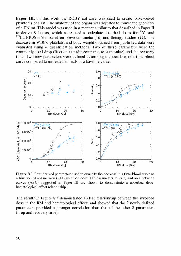
50

Paper III: In this work the ROBY software was used to create voxel-based phantoms of a rat. The anatomy of the organs was adjusted to mimic the geometry of a BN rat. This model was used in a manner similar to that described in Paper II to derive S factors, which were used to calculate absorbed doses for 90Y- and 177Lu-BR96-mAbs based on previous kinetic (10) and therapy studies (11). The decrease in WBCs, platelets, and body weight obtained from published data were evaluated using 4 quantification methods. Two of these parameters were the commonly used drop (fraction at nadir compared to start value) and the recovery time. Two new parameters were defined describing the area loss in a time-blood curve compared to untreated animals or a baseline value.

Figure 8.3. Four derived parameters used to quantify the decrease in a time-blood curve as a function of red marrow (RM) absorbed dose. The parameters severity and area between curves (ABC) suggested in Paper III are shown to demonstrate a absorbed dose-hematological effect relationship.

The results in Figure 8.3 demonstrated a clear relationship between the absorbed dose in the RM and hematological effects and showed that the 2 newly defined parameters provided a stronger correlation than that of the other 2 parameters (drop and recovery time).

0 10 20 30BM dose [Gy]

0

20

40

60

Day

s to

rec

over

y

177Lu

90Y

0 10 20 30BM dose [Gy]

0.0

0.2

0.4

0.6

0.8

1.0

Sev

erity

177Lu (r=0.90)

90Y (r=0.94)

0 10 20 30BM dose [Gy]

0

5.0•103

1.0•104

1.5•104

2.0•104

AB

C [p

late

lets

loss

*109 /L

*day

s]

177Lu (r=0.97)

90Y (r=0.92)

0 10 20 30BM dose [Gy]

0.0

0.2

0.4

0.6

0.8

1.0

Dro

p

177Lu (r=0.77)

90Y (r=0.95)

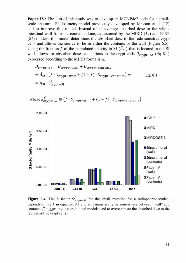
51

Paper IV: The aim of this study was to develop an MCNP4c2 code for a small-scale anatomic SI dosimetry model previously developed by Jönsson et al. (12) and to improve this model. Instead of an average absorbed dose to the whole intestinal wall from the contents alone, as assumed by the MIRD (14) and ICRP (21) models, this model determines the absorbed dose to the radiosensitive crypt cells and allows the source to be in either the contents or the wall (Figure 6.5). Using the fraction of the cumulated activity in SI ( ) that is located in the SI wall allows for absorbed dose calculations to the crypt cells ← (Eq 8.1) expressed according to the MIRD formalism. ← = ← + ← = = · · ← + (1 − ) · ← = = A · S ←

Eq. 8.1

, where ← ≡ · ← + (1 − ) · ←

Figure 8.4. The S factor ← for the small intestine for a radiopharmaceutical depends on the in equation 8.1 and will numerically be somewhere between “wall” and “contents,” suggesting that traditional models tend to overestimate the absorbed dose to the radiosensitive crypt cells.

0.0E+00

5.0E-05

1.0E-04

1.5E-04

2.0E-04

99m-Tc 111-In 131-I 67-Ga 90-Y

S fa

ctor

(mG

y M

Bq-

1 s-1

)

ICRP

MIRD

MIRDOSE 3

Jönsson et al (wall)

Jönsson et al (contents)

Paper IV (wall)

Paper IV (contents)

52

In conclusion, our investigations show that the MIRD and ICRP models clearly overestimate the absorbed dose to the radiosensitive crypt cells in the SI, and that the uptake in the wall must be considered.

Paper V: For many years, the internal dosimetry community has recognized the need for a more detailed, cell-level testicular dosimetry. This paper presents such a small-scale dosimetry model for the calculation of S factors for a number of source-target configurations within testicular tissue. The geometry was based on concentric cylinders representing the cell layers in the seminiferous tubules, replicated in a hexagonal pattern (Figure 6.6).

Electron transport was performed one source region at a time using the new energy straggling logic option in MCNP5 1.51.

Figure 8.5. Ratio of the absorbed doses per region to the absorbed dose to whole-testis from activity in; (left) the interstitial tissue and (right) spermatogonia. The source and target regions (1-9) correspond to the tissues depicted in Figure 3.3 and Figure 6.6. The horizontal line at y=1 is thus equal to the average absorbed dose in whole-testis.

This research shows that the absorbed dose to the radiosensitive spermatogonia (Figure 8.5, region 3) is highly dependent on the emission characteristics of the radionuclide and the biodistribution within the testis. The data also demonstrated that the traditionally used mean absorbed dose cannot predict the correct dose to spermatogonia. The extreme case is for the very-low-energy emitter 125I. If activity uptake is in the spermatogonia, this dosimetry model gives a 4.74 times higher absorbed dose to the spermatogonia than that of the standard whole-testis absorbed dose, whereas if the activity is in the interstitial tissue, the absorbed dose is 0.39 times the standard whole-testis absorbed dose.

Source: region 1

1 2 3 4 5 6 7 8 9125I211At99Tcm

111In177Lu131I18F90Y

Source: region 3

1 2 3 4 5 6 7 8 9125I211At99Tcm

111In177Lu131I18F90Y

53

9. Conclusion

Large differences in absorbed dose calculations can occur depending on the dosimetry model being used. When the dimension of target regions can no longer be regarded as large compared to the electron range, the electron transport in the calculation must be included to obtain correct self-doses and cross-doses. Because these absorbed doses vary significantly depending on the geometry of an object, the geometry must be modeled carefully to calculate a correct absorbed dose to the radiobiologically interesting target. If the absorbed dose can be well calculated this will have a great impact when relating absorbed doses to radiobiology.

In Paper III we present a novel method for a quantitative correlation between the reduction in peripheral WBC and platelet concentrations as a function of the absorbed dose to the RM. This study demonstrates that a carefully developed dosimetry model can provide a good correlation for hematological toxicity as well as changes in body weight. We believe that the mathematical framework may be useful if incorporated into future comparative studies of the hematopoietic system response to different radiolabeled agents. The framework is applicable to animals as well as humans exposed to ionizing radiation.

54

10. Future/Vision

The recent increase in the development of realistic detailed phantoms and auto-segmentations will lead to vast improvements for the macro-dosimetry. Small-scale anatomic dosimetry models still need to rely on a geometrical model that properly describes the “organized chaos” cell structure in a tissue.

We believe that some of our proposed improvements in small-animal models are of great importance for future studies. As discussed in Paper II, tumor activity is considered homogeneously distributed. Many tumors are known to have a highly vascularized outer shell and a poorly vascularized or necrotic core (105, 135). These features affect the self-dose, especially for high-energy electrons, whereas the cross-dose from other tissues is less affected. A poorly vascularized core also leads to more radioresistant cells. Future work may, therefore, include a tumor model that is based on spherical layers or that incorporates 3D activity distribution data from high-resolution imaging systems, such as digital ARG, µSPECT, and µPET.

In Paper III, we found a correlation between the absorbed dose and several hematological effects. A substantial amount of data has been gathered on tumor properties and tumor shrinkage after treatment with radiolabeled mAbs. Based on the imaging of these properties using µSPECT and digital ARG, we will perform accurate dosimetry with the aim of establishing correlation with biological effects.

The RM in mice or rats is, in contrast to that in humans, distributed in almost all skeletal cavities. Most of the RM can be assumed to be homogeneously distributed within the cortical bone, but in regions such as the spine and the proximal and distal ends of long bones, the RM is located in cavities that are surrounded by trabecular bone. We have developed an MCNP routine that takes this geometry into account. The emitted particles are simulated in a coarse voxel phantom, but when the particles enter volumes that require a higher spatial resolution, the code uses a representation with finer voxel dimensions. This method is an analog to the paired image radiation transport technique mentioned earlier. The code works in practice but is computationally inefficient when using MCNP5. Therefore, we cannot benefit from the improved energy logic needed for these small voxels. If in the near future the development of MCNP codes does not improve voxel-based calculations, we plan to adopt a more efficient code, such as Penelope, for this purpose.

In paper V we calculated the absorbed dose to the various cell layers in the seminiferous tubule in the testis. Using imaging techniques, we have investigated

55

distributions of various radiopharmaceuticals. In the future, we plan to use this model to calculate absorbed doses to the highly radiosensitive spermatogonia with the purpose of correlating the absorbed dose from radiopharmaceuticals and radionuclides to biological effects in the testis.

Accurate biological effect–absorbed dose relationships in vivo in RNT are difficult to obtain mainly because of large uncertainties in the absorbed dose calculations and measured biological parameters. If the dosimetry models are improved by accounting for heterogeneities and including better definitions of the primary targets of radiation, then correlation may be more solid and significant. This outcome probably requires that radiobiological considerations be taken into account to fully understand the effects of RNT.

Since the paper by Barone et al. (136) in 2005 that demonstrated a stronger correlation between kidney toxicity in peptide receptor radionuclide therapy and the calculated biological effective dose (BED) compared to the absorbed dose, many investigators have focused on the use of BED (Eq 9.1). This quantity is derived from the linear-quadratic model of the survival fraction ( )of cells following an acute irradiation described earlier (Eq 1.1).

= − ln ( ) Eq. 9.1

In contrast to fractionated radiotherapy, in which the time between fractions is long enough to allow for the complete repair of sublethal damages, the absorbed dose in RNTs is delivered continuously. The dose rate must thus be considered as well as the repair time of the double-strand breaks to calculate BED. The dosimetry community seems to agree that the use of biological models has several advantages. An intense debate regarding the usefulness of the BED has occurred in the literature during recent years (137-144), partly because the relevance of the / ratios obtained from external radiation therapy have not yet been proven for RNT. If / ratios are derived from inadequate dosimetry, then it is questionable whether they can be used in more sophisticated dosimetry models on the cell level, which accounts for the fact that different cells can show different sensitivities to radiation and abilities for repair. It is thus possible that the derived / ratios are specific to a particular radionuclide or radiopharmaceutical. Thus, it is important to encourage the development of more accurate and realistic dosimetry models for both large organs as well as tissues/cells/cell structures and from these make use of biological models that can establish correlations to biological effects and responses.

56

Acknowledgements

During the process of writing this thesis I have received help and support from several people, for which I am very thankful. I would like to express my gratitude to all of you and in particular to:

My main supervisor, Bo-Anders Jönsson, who not only supervised me through this thesis, but also introduced me to the field of Medical Radiation Physics when I should have done my Master of Science thesis in physics, a detour well worth the extra time.

My co-supervisor, Michael Ljungberg, for all the discussions and your huge support, not to mention all the help with various computer technicalities.

Sven-Erik Strand, who formally was not my supervisor but nevertheless acted as one, supplying me with articles and always giving me positive feedback.

All of the co-authors of the papers for providing expertise in different fields.

Dr. Paul Segars, Department of Radiology, Duke University for all your help with the MOBY and ROBY phantoms.

All my friends and colleagues at the Department of Medical Radiation Physics for pleasant company and help in many different areas. A special thank to the members of the SST group: Anders Sandell, Anders Örbom, Bo-Anders Jönsson, Cecilia Hindorf, David Minarik, Gustav Brolin, Gustav Grafström, Henrik Hussein El-Ali, Johan Gustafsson, Jonas Ahlstedt, Jonathan Siikanen, Karin Wingårdh, Katarina Sjögreen-Gleisner, Kaj Ljunggren, Lena Jönsson, Michael Ljungberg, Mikael Peterson, Oskar Vilhelmsson Timmermand, Pontus Kjellman, Renata Madru, Suaad Meerkhan, Sven-Erik Strand and Thuy Tran.

My friends and colleagues at the Radiation Physics, Skåne University Hospital, for bringing me many enjoyable moments and the insight to radionuclide therapies in practice.

My parents and sisters for all your love and support during the years.

My daughter Tuva, my dear wife Josefin and our soon-to-be-born daughter for all the love and joy you bring to my life.

This work was generously supported by; The Swedish Cancer Foundation, the Swedish Radiation Safety Authority, the Swedish Society of Radiation Physics, Lund University Hospital Donation Funds, The Gunnar Nilsson’s Foundation, Mrs. Berta Kamprad Foundation, John and Augusta Persson’s Foundation for Medical Research.

57

References

1. Tennvall J, Brans B. EANM procedure guideline for 32P phosphate treatment of myeloproliferative diseases. Eur J Nucl Med Mol Imaging. 2007;34:1324-1327.

2. Davies AJ. Radioimmunotherapy for B-cell lymphoma: Y90 ibritumomab tiuxetan and I131 tositumomab. Oncogene. 2007;26:3614-3628.

3. Otte A, Jermann E, Behe M, Goetze M, Bucher HC, Roser HW, Heppeler A, Mueller-Brand J, Maecke HR. DOTATOC: a powerful new tool for receptor-mediated radionuclide therapy. Eur J Nucl Med. 1997;24:792-795.

4. Otte A, Herrmann R, Macke HR, Muller-Brand J. [Yttrium 90 DOTATOC: a new somatostatin analog for cancer therapy of neuroendocrine tumors]. Praxis (Bern 1994). 1999;88:1263-1268.

5. Cremonesi M, Ferrari M, Zoboli S, et al. Biokinetics and dosimetry in patients administered with (111)In-DOTA-Tyr(3)-octreotide: implications for internal radiotherapy with (90)Y-DOTATOC. Eur J Nucl Med. 1999;26:877-886.

6. Kwekkeboom DJ, Bakker WH, Kam BL, et al. Treatment of patients with gastro-entero-pancreatic (GEP) tumours with the novel radiolabelled somatostatin analogue [177Lu-DOTA(0),Tyr3]octreotate. Eur J Nucl Med Mol Imaging. 2003;30:417-422.

7. Hall EJ. Radiobiology for the radiologist: Lippincott Williams & Wilkins; 2011. 8. Mothersill C, Seymour C. Radiation-induced bystander effects: past history and

future directions. Radiat Res. 2001;155:759-767. 9. Rees GJ. Abscopal regression in lymphoma: a mechanism in common with total body

irradiation? Clinical radiology. 1981;32:475-480. 10. Wang Z, Mårtensson L, Nilsson R, Bendahl P-O, Lindgren L, Ohlsson T, Sjögren H-

O, Strand S-E, Tennvall J. Blood Pharmacokinetics of Various Monoclonal Antibodies Labeled with a New Trifunctional Chelating Reagent for Simultaneous Conjugation with 1,4,7,10-Tetraazacyclododecane-N,N',N'',N'''-Tetraacetic Acid and Biotin before Radiolabeling. Clinical Cancer Research. 2005;11:7171s-7177s.

11. Mårtensson L, Wang Z, Nilsson R, Ohlsson T, Senter P, Sjögren HO, Strand SE, Tennvall J. Determining maximal tolerable dose of the monoclonal antibody BR96 labeled with 90Y or 177Lu in rats: establishment of a syngeneic tumor model to evaluate means to improve radioimmunotherapy. Clin Cancer Res. 2005;11:7104-7108.

12. Jönsson L, Liu X, Jönsson BA, Ljungberg M, Strand SE. A dosimetry model for the small intestine incorporating intestinal wall activity and cross-doses. J Nucl Med. 2002;43:1657-1664.

13. ICRU. Fundamental Quantities and Units for Ionizing Radiation 2011. Report 85, Vol. 11 No. 1.

58

14. Snyder WS, Ford MR, Warner GG, Watson SB. "S," Absorbed Dose per Unit Cumulated Activity for Selected Radionuclides and Organs.: Society of Nuclear Medicine; 1975.

15. Bolch WE, Eckerman KF, Sgouros G, Thomas SR. MIRD pamphlet No. 21: a generalized schema for radiopharmaceutical dosimetry--standardization of nomenclature. J Nucl Med. 2009;50:477-484.

16. Hindorf C, Linden O, Stenberg L, Tennvall J, Strand SE. Change in tumor-absorbed dose due to decrease in mass during fractionated radioimmunotherapy in lymphoma patients. Clin Cancer Res. 2003;9:4003S-4006S.

17. Berger MJ. Distribution of absorbed dose around point sources of electrons and beta particles in water and other media. J Nucl Med. 1971:Suppl 5:5-23.

18. Ljungberg M, Sjogreen-Gleisner K. The accuracy of absorbed dose estimates in tumours determined by quantitative SPECT: a Monte Carlo study. Acta Oncol. 2011;50:981-989.

19. Snyder WS, Ford MR, Warner GG. Estimates of specific fractions for photon sources uniformly distributed in various organs of a heterogeneous phantom. : Society of Nuclear Medicine; 1978.

20. Loevinger RF, Budinger T, Watson EE. MIRD Primer for Absorbed Dose Calculations New York: The Society of Nuclear Medicine Inc; 1988.

21. ICRP. Limits for intakes of radionuclides by workers. Oxford: International Commission on Radiological Protection; 1979. ICRP report 30.

22. Human alimentary tract model for radiological protection. ICRP Publication 100. A report of The International Commission on Radiological Protection. Ann ICRP. 2006;36:25-327, iii.

23. Roeske JC, Aydogan B, Bardies M, Humm JL. Small-scale dosimetry: challenges and future directions. Seminars in nuclear medicine. 2008;38:367-383.

24. ICRU. Absorbed-Dose Specification in Nuclear Medicine 2002. ICRU Report 67, Vol. 2, No. 1.

25. Fisher D, Rajon D, Breitz H, Goris M, Bolch W, Knox S. Dosimetry model for radioactivity localized to intestinal mucosa. Cancer Biother Radiopharm. 2004;19:293-307.

26. Howell RW, Rao DV, Bouchet LG, Bolch W, Goddu SM. MIRD cellular S values: self-absorbed dose per unit cumulated activity for selected radionuclides and monoenergetic electron and alpha particle emitters incorporated into different cell compartments: Society of Nuclear Medicine; 1997.

27. Siegel JA, Wessels BW, Watson EE, et al. Bone marrow dosimetry and toxicity for radioimmunotherapy. Antibody Immunconj Radiopharm. 1990;3:213-233.

28. Fliedner TM, Graessle D, Paulsen C, Reimers K. Structure and function of bone marrow hemopoiesis: mechanisms of response to ionizing radiation exposure. Cancer Biother Radiopharm. 2002;17:405-426.

29. Beddoe AH, Darley PJ, Spiers FW. Measurements of trabecular bone structure in man. Phys Med Biol. 1976;21:589-607.

30. ICRP Publication 70: Basic Anatomical and Physiological Data for Use in Radiological Protection: The Skeleton. 1995 25.

31. Eckerman KF, Stabin MG. Electron absorbed fractions and dose conversion factors for marrow and bone by skeletal regions. Health Phys. 2000;78:199-214.

59

32. Sgouros G. Bone marrow dosimetry for radioimmunotherapy: theoretical considerations. J Nucl Med. 1993;34:689-694.

33. Wessels BW, Bolch WE, Bouchet LG, Breitz HB, Denardo GL, Meredith RF, Stabin MG, Sgouros G. Bone marrow dosimetry using blood-based models for radiolabeled antibody therapy: a multiinstitutional comparison. J Nucl Med. 2004;45:1725-1733.

34. Michelsen K. Determination of Inulin, Albumin and Erythrocyte Spaces in the Bone Marrow of Rabbits. Acta Physiolog Scand. 1969;77:28-35.

35. Cremonesi M, Ferrari M, Bodei L, Tosi G, Paganelli G. Dosimetry in Peptide Radionuclide Receptor Therapy: A Review. J Nucl Med. 2006;47:1467-1475.

36. Sgouros G. Blood and Bone Marrow Dosimetry in Radioiodine Therapy of Thyroid Cancer. J Nucl Med. 2005;46:899-900.

37. Hindorf C, Linden O, Tennvall J, Wingårdh K, Strand SE. Time dependence of the activity concentration ratio of red marrow to blood and implications for red marrow dosimetry. Cancer. 2002;94:1235-1239.

38. Spiers FW, Beddoe AH, King SD. The absorbed dose to bone marrow in the treatment of polycythaemia by 32P. Br J Radiol. 1976;49:133-140.

39. Whitwell JR, Spiers FW. Calculated beta-ray dose factors for trabecular bone. Phys Med Biol. 1976;21:16-38.

40. Spiers FW, Beddoe AH. 'Radial' scanning of trabecular bone: consideration of the probability distributions of path lengths through cavities and trabeculae. Phys Med Biol. 1977;22:670-680.

41. Spiers FW, Beddoe AH, Whitwell JR. Mean skeletal dose factors for beta-particle emitters in human bone. Part I: volume-seeking radionuclides. Br J Radiol. 1978;51:622-627.

42. Spiers FW, Whitwell JR, Beddoe AH. Calculated dose factors for the radiosensitive tissues in bone irradiated by surface-deposited radionuclides. Phys Med Biol. 1978;23:481-494.

43. Beddoe AH, Spiers FW. A comparative study of the dosimetry of bone-seeking radionuclides in man, rhesus monkey, beagle, and miniature pig. Radiat Res. 1979;80:423-439.

44. Stabin MG. MIRDOSE: personal computer software for internal dose assessment in nuclear medicine. J Nucl Med. 1996;37:538-546.

45. Stabin MG, Siegel JA. Physical models and dose factors for use in internal dose assessment. Health Phys. 2003;85:294-310.

46. Stabin MG, da Luz LC. Decay data for internal and external dose assessment. Health Phys. 2002;83:471-475.

47. Shah PA, Bolch WE, Rajon DA, Patton PA, Jokisch DA. A Paired-Image Radiation Transport Model for Skeletal Dosimetry. J Nucl Med. 2005;46:344-353.

48. Hough M, Johnson P, Rajon D, Jokisch D, Lee C, Bolch W. An image-based skeletal dosimetry model for the ICRP reference adult male--internal electron sources. Phys Med Biol. 2011;56:2309-2346.

49. Bolch WE, Patton PW, Rajon DA, Shah AP, Jokisch DW, Inglis BA. Considerations of marrow cellularity in 3-dimensional dosimetric models of the trabecular skeleton. J Nucl Med. 2002;43:97-108.

50. Watchman CJ, Jokisch DW, Patton PW, Rajon DA, Sgouros G, Bolch WE. Absorbed fractions for alpha-particles in tissues of trabecular bone: considerations of marrow cellularity within the ICRP reference male. J Nucl Med. 2005;46:1171-1185.

60

51. Pichardo JC, Milner RJ, Bolch WE. MRI measurement of bone marrow cellularity for radiation dosimetry. J Nucl Med. 2011;52:1482-1489.

52. Nicholas D. Hematologic consequences of exposure to ionizing radiation. Experimental Hematology. 2002;30:513-528.

53. National Research Council NRC. HEALTH RISKS FROM EXPOSURE TO LOW LEVELS OF IONIZING RADIATION - BEIR VII PHASE 2. Washington DC: National Research Council; 2006.

54. UNSCEAR 2006 REPORT Vol. I. Effects of ionizing radiation: Annex A - Epidemiological studies of radiation and cancer: UNSCEAR; 2006.

55. Potten CS. Radiation, the ideal cytotoxic agent for studying the cell biology of tissues such as the small intestine. RadiatRes. 2004;161:123-136.

56. Rowley MJ, Leach DR, Warner GA, Heller CG. Effect of Graded Doses of Ionizing Radiation on the Human Testis. Radiat Res. 1974;59:665-678.

57. ICRP. Nonstochastic Effects of Ionizing Radiation. ICRP Publication 41. Ann ICRP. 1984;14.

58. Mescher AL. Junqueira's Basic Histology - Text and Atlas, 12th Edition. 12th ed: Mc Graw Hill Medical; 2009.

59. Oakberg EF. Duration of spermatogenesis in the mouse and timing of stages of the cycle of the seminiferous epithelium. Am J Anat. 1956;99:507-516.

60. Meistrich ML. Critical components of testicular function and sensitivity to disruption. Biol Reprod. 1986;34:17-28.

61. Rao DV, Narra V, Howell RW, Lanka V, Sastry KSR. Induction of sperm head abnormalities by incorporated radionuclides: Dependance on subcellular distribution, type of radiation, dose rate, and presence of radioprotectors. Radiat Res. 1991;125:89-97.

62. Meistrich ML, Samuels RC. Reduction in sperm levels after testicular irradiation of the mouse: a comparison with man. Radiat Res. 1985;102:138-147.

63. Meistrich M, Reid B, Barcellona W. Changes in Sperm Nuclei During Spermiogenesis and Epididymal Maturation. Exp Cell Res. 1976;99:72-78.

64. Hendry JH. Survival of cells in mammalian tissues after low doses of irradiation: a short review. Int J Radiat Biol. 1988;53:89-94.

65. Yousif L, Blettner M, Hammer GP, Zeeb H. Testicular cancer risk associated with occupational radiation exposure: a systematic literature review. Journal of Radiological Protection. 2010;30:389.

66. UNSCEAR 2010 REPORT. Summary of low-dose radiation effects on health: UNSCEAR; 2010.

67. Stabin M, da Luz LC. Decay data for internal and external dose assessment. Health Phys. 2002;83:471-475.

68. Willmann JK, van Bruggen N, Dinkelborg LM, Gambhir SS. Molecular imaging in drug development. Nature reviews Drug discovery. 2008;7:591-607.

69. Fueger BJ, Czernin J, Hildebrandt I, Tran C, Halpern BS, Stout D, Phelps ME, Weber WA. Impact of animal handling on the results of 18F-FDG PET studies in mice. J Nucl Med. 2006;47:999-1006.

70. Taschereau R, Chow PL, Chatziioannou AF. Monte carlo simulations of dose from microCT imaging procedures in a realistic mouse phantom. Med Phys. 2006;33:216-224.

61

71. Jönsson BA, Strand, S. E., Emanuelsson, H., Larsson, B. S. Tissue, cellular, and subcellular distribution of indium radionuclides in the rat. Biophysical Aspects of Auger Processes, AAPM Symposium Series No. 8. Woodbury, NY: American Institute of Physics; 1992:249-272.

72. Örbom A, Dahlbom M, Olafsen T, Wu AM, Strand SE. Serial digital autoradiography with a silicon strip detector as a high resolution imaging modality for TRT dosimetry. Paper presented at: Nuclear Science Symposium Conference Record, 2007. NSS '07. IEEE; Oct. 26 2007-Nov. 3 2007, 2007.

73. Fisher HLJ, Snyder WS. Variation of dose delivered by 137Cs as a function of body size from a source of gamma rays distributed uniformly in an organ, ORNL-4168. In: Laboratory ORN, ed. Oak Ridge, TN; 1967:221.

74. Snyder WS, Ford MR, Warner GG, Fisher HLJ. MIRD Pamphlet #5 Revised: Estimates of Absorbed Fractions for Monoenergetic Photon Sources Uniformly Distributed in Various Organs of a Heterogeneous Phantom J Nucl Med. 1969:Suppl Number 3.

75. ICRP Publication 23: Report of the task group on Reference Man. Annals of the ICRP/ICRP Publication. 1975;23.

76. Cristy M, Eckerman KF. Specific absorbed fractions of energy at various ages from internal photon sources. Oak Ridge, TN: Oak Ridge National Laboratory; 1987

77. Knöös T, Nilsson M, Ahlgren L. A method for conversion of Hounsfield number to electron density and prediction of macroscopic pair production cross-sections. Radiother Oncol. 1986;5:337-345.

78. Rajon DA, Jokisch DW, Patton PW, Shah AP, Watchman CJ, Bolch WE. Voxel effects within digital images of trabecular bone and their consequences on chord-length distribution measurements. Phys Med Biol. 2002;47:1741-1759.

79. Rajon DA, Patton PW, Shah AP, Watchman CJ, Bolch WE. Surface area overestimation within three-dimensional digital images and its consequence for skeletal dosimetry. Med Phys. 2002;29:682-693.

80. Zubal IG, Harrell CR, Smith EO, Rattner Z, Gindi G, Hoffer PB. Computerized three-dimensional segmented human anatomy. Med Phys. 1994;21:299-302.

81. Caon M, Bibbo G, Pattison J. An EGS4-ready tomographic computational model of a 14-year-old female torso for calculating organ doses from CT examinations. Phys Med Biol. 1999;44:2213-2225.

82. Petoussi-Henss N, Zanki M, Fill U, Regulla D. The GSF family of voxel phantoms. Phys Med Biol. 2002;47:89-106.

83. Kramer R, Khoury HJ, Vieira JW, Lima VJ. MAX06 and FAX06: update of two adult human phantoms for radiation protection dosimetry. Phys Med Biol. 2006;51:3331-3346.

84. Spitzer VM, Whitlock DG. Atlas of the Visible Human Male. Sudbury, MA, USA: Joner and Bartlett Publishers; 1998.

85. Kramer R, Khoury HJ, Vieira JW, Kawrakow I. Skeletal dosimetry for external exposure to photons based on microCT images of spongiosa from different bone sites. Phys Med Biol. 2007;52:6697-6716.

86. ICRP publication 89: Basic Anatomical and Physiological Data for Use in Radiological Protection - Reference Values. Ann ICRP. 2002;32:5-265.

87. ICRP Publication 110: Adult Reference Computational Phantoms. Ann ICRP. 2009;39

62

88. Segars WP, Lalush DS, Tsui BMW. Modeling respiratory mechanics in the MCAT and spline-based MCAT phantoms. Nuclear Science, IEEE Transactions on. 2001;48:89-97.

89. Segars WP. Development and Application of the New Dynamic NURBS-based Cardiac-Torso (NCAT) Phantom [PhD thesis]. Chapel Hill, The University of North Carolina; 2001.

90. Segars WP, Tsui BM, Frey EC, Johnson GA, Berr SS. Development of a 4-D digital mouse phantom for molecular imaging research. Mol Imaging Biol. 2004;6:149-159.

91. Keenan MA, Stabin MG, Segars WP, Fernald MJ. RADAR realistic animal model series for dose assessment. J Nucl Med. 2010;51:471-476.

92. Segars WP, Sturgeon G, Mendonca S, Grimes J, Tsui BM. 4D XCAT phantom for multimodality imaging research. Med Phys. 2010;37:4902-4915.

93. Zhang J, Xu GX, Shi C, Fuss M. Development of a geometry-based respiratory motion-simulating patient model for radiation treatment dosimetry. Journal of applied clinical medical physics / American College of Medical Physics. 2008;9:2700.

94. Lee C, Lodwick D, Hasenauer D, Williams JL, Bolch WE. Hybrid computational phantoms of the male and female newborn patient: NURBS-based whole-body models. Phys Med Biol. 2007;52:3309-3333.

95. Lee C, Lodwick D, Hurtado J, Pafundi D, Williams JL, Bolch WE. The UF family of reference hybrid phantoms for computational radiation dosimetry. Phys Med Biol. 2010;55:339-363.

96. Xu XG, Eckerman KF. Handbook of Anatomical Models for Radiation Dosimetry. Boca Raton: Taylor & Francis; 2009.

97. Xu XG, Taranenko V, Zhang J, Shi C. A boundary-representation method for designing whole-body radiation dosimetry models: pregnant females at the ends of three gestational periods--RPI-P3, -P6 and -P9. Phys Med Biol. 2007;52:7023-7044.

98. Zhang J, Na YH, Caracappa PF, Xu XG. RPI-AM and RPI-AF, a pair of mesh-based, size-adjustable adult male and female computational phantoms using ICRP-89 parameters and their calculations for organ doses from monoenergetic photon beams. Phys Med Biol. 2009;54:5885-5908.

99. Cassola VF, Lima VJ, Kramer R, Khoury HJ. FASH and MASH: female and male adult human phantoms based on polygon mesh surfaces: I. Development of the anatomy. Phys Med Biol. 2010;55:133-162.

100. Kramer R, Cassola VF, Khoury HJ, Vieira JW, Lima VJ, Brown KR. FASH and MASH: female and male adult human phantoms based on polygon mesh surfaces: II. Dosimetric calculations. Phys Med Biol. 2010;55:163-189.

101. Kim CH, Jeong JH, Bolch WE, Cho KW, Hwang SB. A polygon-surface reference Korean male phantom (PSRK-Man) and its direct implementation in Geant4 Monte Carlo simulation. Phys Med Biol. 2011;56:3137-3161.

102. Hui TE, Fisher DR, Kuhn JA, Williams LE, Nourigat C, Badger CC, Beatty BG, Beatty JD. A mouse model for calculating cross-organ beta doses from yttrium-90-labeled immunoconjugates. Cancer. 1994;73:951-957.

103. Muthuswamy MS, Roberson PL, Buchsbaum DJ. A mouse bone marrow dosimetry model. J Nucl Med. 1998;39:1243-1247.

104. Yoriyaz H, Stabin MG. Electron and photon transport in a model of a 30 g mouse. J Nucl Med. 1997;38:228.

63

105. Flynn AA, Green AJ, Pedley RB, Boxer GM, Boden R, Begent RH. A mouse model for calculating the absorbed beta-particle dose from (131)I- and (90)Y-labeled immunoconjugates, including a method for dealing with heterogeneity in kidney and tumor. RadiatRes. 2001;156:28-35.

106. Hindorf C, Ljungberg M, Strand SE. Evaluation of parameters influencing S values in mouse dosimetry. J Nucl Med. 2004;45:1960-1965.

107. Kolbert KS, Watson T, Matei C, Xu S, Koutcher JA, Sgouros G. Murine S factors for liver, spleen, and kidney. J Nucl Med. 2003;44:784-791.

108. Stabin MG, Peterson TE, Holburn GE, Emmons MA. Voxel-based mouse and rat models for internal dose calculations. J Nucl Med. 2006;47:655-659.

109. Bitar A, Lisbona A, Thedrez P, Sai MC, Le FD, Barbet J, Bardies M. A voxel-based mouse for internal dose calculations using Monte Carlo simulations (MCNP). Phys Med Biol. 2007;52:1013-1025.

110. Bitar A, Lisbona A, Bardies M. S-factor calculations for mouse models using Monte-Carlo simulations. Q J Nucl Med Mol Imaging. 2007;51:343-351.

111. Hindorf C, Ljungberg M, Strand SE. Dosimetric model for mice and rats [abstract]. J Nucl med. 2003;44(suppl).

112. Konijnenberg MW, Bijster M, Krenning EP, De Jong M. A stylized computational model of the rat for organ dosimetry in support of preclinical evaluations of peptide receptor radionuclide therapy with (90)Y, (111)In, or (177)Lu. J Nucl Med. 2004;45:1260-1269.

113. Klein O, Nishina T. Über die Streuung von Strahlung durch freie Elektronen nach der neuen relativistischen Quantendynamik von Dirac Zeitschrift für Physik A Hadrons and Nuclei. 1929;52:853-868.

114. Kahn H. Applications of Monte Carlo: AEC-3259 The Rand Corporation; 1956. 115. Biggs F, Mendelsohn LB, Mann JB. Hartree-Fock Compton Profiles for the

Elements. Atomic Data and Nuclear Data Tables. 1975;16:201-309. 116. Berger MJ. Monte Carlo Calculation of the Penetration and Diffusion of Fast

Charged Particles. In: Alder B, Fernbach S, Rotenberg M, eds. Methods in Computational Physics,Vol. 1. New York: Academic Press; 1963:135.

117. Goudsmit S, Saunderson JL. Multiple Scattering of Electrons. Phys Rev. 1940;57:24-29.

118. Landau L. On the Energy Loss of Fast Particles by Ionization. J Phys (USSR). 1944;8:201.

119. Lewis HW. Multiple scattering in an infnite medium. Phys Rev. 1950;78:526-529. 120. Kawrakow I, Rogers DW. The EGSnrc code system: Monte Carlo simulations

electron and photon transport. National Research Council of Canada, Ottawa 2001. NRCC Report PIRS-701.

121. Sempau J, Acosta E, Baro J, Fernández-Varea JM, Salvat F. An algorithm for Monte Carlo simulation of coupled electron-photon transport. Nuclear Instruments and Methods in Physics Research Section B: Beam Interactions with Materials and Atoms. 1997;132:377-390.

122. Salvat F, Fernández-Varea JM, Sempau J. PENELOPE-2011, A Code System for Monte Carlo Simulation of Electron and Photon Transport. Issy-les-Moulineaux: OECD Nuclear Energy Agency; 2011.

123. Agostinelli S, Allison J, Amako K, et al. G4--a simulation toolkit. Nucl Instrum Meth A. 2003;506:250-303.

64

124. Allison J, Amako K, Apostolakis J, et al. Geant4 developments and applications. Nuclear Science, IEEE Transactions on. 2006;53:270-278.

125. Jan S, et al. GATE: a simulation toolkit for PET and SPECT. Phys Med Biol. 2004;49:4543.

126. X-5 Monte Carlo Team. MCNP - A General Monte Carlo N-Particle Transport Code, Version 5, Volume I: Overview and theory, Los Alamos National Laboratory report LA-UR-03-1987.

127. Hendricks JS. MCNPX, VERSION 2.6.A. Vol LA-UR-05-8225. Los Alamos, NE: Los Alamos National Laboratory; 2005.

128. Seltzer SM, Berger MJ. An Overview of ETRAN Monte Carlo Methods. In: Jenkins TM, Nelson WR, Rindi A, eds. Monte CarloTransport of Electrons and Photons. New York: Plenum Press; 1988:153.

129. Cullen DE, Hubbell JH, Kissel LD. EPDL97: The Evaluated Photon Data Library,‘97 Version. Lawrence Livermore National Laboratory UCRL-50400. 1997;6, Rev. 5.

130. Everett CJ, Cashwell ED. MCP Code Fluorescence-Routine Revision, Los Alamos Scientific Laboratory report LA-5240-MS May 1973.

131. Koblinger L. Direct Sampling from the Klein-Nishina Distribution for Photon Energies Above 1.4 MeV. Nucl Sci Eng. 1975;56:218

132. Halbleib J. Structure and Operation of the ITS Code System. In: Jenkins TM, Nelson WR, Rindi A, eds. Monte Carlo Transport of Electrons and Photons. New York: Plenum Press; 1988.

133. Blunk O, Leisegang S. Zum Energieverlust schneller Elektronen in dünnen Schichten. Z Physik. 1950;128:500.

134. Schaart RD, Jansen JT, Zoetelief J, de Leege PF. A comparison of MCNP4C electron transport with ITS 3.0 and experiment at incident energies between 100 keV and 20 MeV: influence of voxel size, substeps and energy indexing algorithm. Phys Med Biol. 2002;47:1459.

135. Nielsen T, Murata R, Maxwell RJ, Stodkilde-Jorgensen H, Ostergaard L, Ley CD, Kristjansen PE, Horsman MR. Non-invasive imaging of combretastatin activity in two tumor models: Association with invasive estimates. Acta Oncol. 2010;49:906-913.

136. Barone R, Borson-Chazot F, Valkema R, et al. Patient-specific dosimetry in predicting renal toxicity with (90)Y-DOTATOC: relevance of kidney volume and dose rate in finding a dose-effect relationship. J Nucl Med. 2005;46 Suppl 1:99S-106S.

137. Wessels BW, Konijnenberg MW, Dale RG, et al. MIRD pamphlet No. 20: the effect of model assumptions on kidney dosimetry and response--implications for radionuclide therapy. J Nucl Med. 2008;49:1884-1899.

138. Siegel JA, Stabin MG, Sharkey RM. Renal dosimetry in peptide radionuclide receptor therapy. Cancer Biother Radiopharm. 2010;25:581-588.

139. Siegel JA, Stabin MG, Sharkey RM. Renal dosimetry: ready for biological effective dose? Cancer Biother Radiopharm. 2010;25:589-591.

140. Lassmann M, Strigari L, Bardiès M. Dosimetry is Alive and Well. Cancer Biother Radiopharm. 2010;25:593-595.

141. Wessels BW, Dale RG, Cremonesi M, Meredith RF, Green AJ, Brill B, Bolch WE, Sgouros G, Thomas SR. Renal dosimetry. Cancer Biother Radiopharm. 2010;25:597-599.

65

142. Siegel JA, Stabin MG, Sharkey RM. Renal dosimetry: ready for biological equivalent dose? Response to medical internal radiation dose and European association of nuclear medicine committee letters. Cancer Biother Radiopharm. 2010;25:763-765.

143. Bodei L, Cremonesi M, Paganelli G. Something More than Estimating Renal Dosimetry. Cancer Biother Radiopharm. 2010;25:767-768.

144. Siegel JA, Stabin MG, Sharkey RM. Renal dosimetry: ready for BED? Response to the Italian researchers. Cancer Biother Radiopharm. 2011;26:141-142.