Real-time Physics Based Simulation for 3D Computer Graphics

Georgia State UniversityScholarWorks @ Georgia State University

Computer Science Dissertations Department of Computer Science

12-18-2013

Real-time Physics Based Simulation for 3DComputer GraphicsXiao ChenGeorgia State University

Follow this and additional works at: https://scholarworks.gsu.edu/cs_diss

This Thesis is brought to you for free and open access by the Department of Computer Science at ScholarWorks @ Georgia State University. It has beenaccepted for inclusion in Computer Science Dissertations by an authorized administrator of ScholarWorks @ Georgia State University. For moreinformation, please contact [email protected].

Recommended CitationChen, Xiao, "Real-time Physics Based Simulation for 3D Computer Graphics." Thesis, Georgia State University, 2013.https://scholarworks.gsu.edu/cs_diss/79

https://scholarworks.gsu.edu?utm_source=scholarworks.gsu.edu%2Fcs_diss%2F79&utm_medium=PDF&utm_campaign=PDFCoverPages

https://scholarworks.gsu.edu/cs_diss?utm_source=scholarworks.gsu.edu%2Fcs_diss%2F79&utm_medium=PDF&utm_campaign=PDFCoverPages

https://scholarworks.gsu.edu/computer_science?utm_source=scholarworks.gsu.edu%2Fcs_diss%2F79&utm_medium=PDF&utm_campaign=PDFCoverPages

https://scholarworks.gsu.edu/cs_diss?utm_source=scholarworks.gsu.edu%2Fcs_diss%2F79&utm_medium=PDF&utm_campaign=PDFCoverPages

mailto:[email protected]

REAL-TIME PHYSICS BASED SIMULATION FOR 3D COMPUTER GRAPHICS

AT GEORGIA STATE UNIVERSITY

by

XIAO CHEN

Under the Direction of Ying Zhu

ABSTRACT

Restoration of realistic animation is a critical part in the area of computer graphics. The

goal of this sort of simulation is to imitate the behavior of the transformation in real life to the

greatest extent. Physics-based simulation provides a solid background and proficient theories that

can be applied in the simulation. In this dissertation, I will present real-time simulations which

are physics-based in the area of terrain deformation and ship oscillations.

When ground vehicles navigate on soft terrains such as sand, snow and mud, they often

leave distinctive tracks. The realistic simulation of such vehicle-terrain interaction is important

for ground based visual simulations and many video games. However, the existing research in

terrain deformation has not addressed this issue effectively. In this dissertation, I present a new

terrain deformation algorithm for simulating vehicle-terrain interaction in real time. The

algorithm is based on the classic terramechanics theories, and calculates terrain deformation

according to the vehicle load, velocity, tire size, and soil concentration. As a result, this

algorithm can simulate different vehicle tracks on different types of terrains with different

vehicle properties. I demonstrate my algorithm by vehicle tracks on soft terrain.

In the field of ship oscillation simulation, I propose a new method for simulating ship

motions in waves. Although there have been plenty of previous work on physics based fluid-

solid simulation, most of these methods are not suitable for real-time applications. In particular,

few methods are designed specifically for simulating ship motion in waves. My method is based

on physics theories of ship motion, but with necessary simplifications to ensure real-time

performance. My results show that this method is well suited to simulate sophisticated ship

motions in real time applications.

INDEX WORDS: Terrain deformation, Ship oscillation, Virtual reality



by

XIAO CHEN

A Thesis Submitted in Partial Fulfillment of the Requirements for the Degree of

Doctor of Philosophy

In the College of Arts and Sciences

Georgia State University

2013

Copyright by

Xiao Chen

2013



by

XIAO CHEN

Committee Chair: Dr. Ying Zhu

Committee: Dr. G. Scott Owen

Dr. Rajshekhar Sunderraman

Dr. Dajun Dai (Geosciences)

Electronic Version Approved:

Office of Graduate Studies

College of Arts and Sciences

Georgia State University

December 2013

iv

DEDICATION

I would like to dedicate this Doctoral dissertation to my father, Jianrong Chen, my mother,

Xiaoling Song, my grandfather, Mingxin Song, my grandmother, Jifen Zeng and my uncle

Jianping Song. There is no doubt in my mind that without their continued support and counsel I

could not have completed this process.

v

ACKNOWLEDGEMENTS

At first, I would like to express my sincere gratitude to my advisor Dr. Ying Zhu for his

continuous support during my Ph.D research. Besides my advisor, I would like to thank all of my

thesis committee members: Dr. G. Scott Owen, Dr. Rajshekhar Sunderraman, and Dr. Dajun Dai

for their encouragement and advices.

The text of this dissertation includes reprints of the following previously published papers:

Chen, X., Zhu, Y., Shader based polygon stitching and its application in deformable terrain

simulation, Image and Graphics (ICIG), 2011 Sixth International Conference on, pp 885-890

Zhu, Y., Chen, X. and Owen G.S., Terramechanics based terrain deformation for real-time off-

road vehicle simulation, Advances in Visual Computing Lecture Notes in Computer Science

Volume 6938, 2011, pp 431-440

Chen, X., Wang, G. and Zhu, Y., Evaluating a Mobile Pedestrian Safety Application in a Virtual

Urban Environment, VRCAI '12 Proceedings of the 11th ACM SIGGRAPH International

Conference on Virtual-Reality Continuum and its Applications in Industry, pp 175-180

Chen, X., Wang, G. and Zhu, Y., Real-time Simulation of Ship Motions in Waves, Advances in

Visual Computing Lecture Notes in Computer Science Volume 7431, 2012, pp 71-80

Chen, X., Zhu, Y., Real-time Simulation of Vehicle Tracks on Soft Terrain, International

Symposium on Visual Computing 2013, Part I, LNCS 8033 proceedings

vi

TABLE OF CONTENTS

ACKNOWLEDGEMENTS ......................................................................................................... v

TABLE OF CONTENTS ............................................................................................................ vi

LIST OF FIGURES ...................................................................................................................... x

1. INTRODUCTION..................................................................................................................... 1

1.1 Problem Statement.................................................................................................. 1

1.2 My Contributions .................................................................................................... 2

1.3 Organization of This Dissertation ......................................................................... 3

2. PHYSICS IN GAMES AND SIMULATIONS ....................................................................... 3

2.1 Deformable Object .................................................................................................. 5

2.1.1 Terrain Deformation ..................................................................................................... 5

2.1.2 Object Destruction......................................................................................................... 6

2.2 Rigid Body ............................................................................................................... 7

2.3 Motion ...................................................................................................................... 8

2.2.1 Ship Oscillation ............................................................................................................. 8

2.2.2 Little Big Planet ............................................................................................................ 9

2.3 Collision Detection .................................................................................................. 9

2.3.1 Application of Collision Detection ............................................................................. 11

2.4 Particle System ...................................................................................................... 11

2.4.1 Fire .............................................................................................................................. 12

2.4.2 Smoke .......................................................................................................................... 13

vii

2.4.3 Rain.............................................................................................................................. 13

3. TERRAIN DEFORMATION ................................................................................................ 15

3.1 Introduction ........................................................................................................... 15

3.2 Previous Work of Terrain Deformation ............................................................. 16

3.2.1 Terrain Compression .................................................................................................. 16

3.2.2 Tire Tread Pattern ....................................................................................................... 20

3.2.3 Debris ........................................................................................................................... 21

3.3 Terrain-mechanics ................................................................................................ 21

3.3.1 Theories on Vehicle-Terrain Interaction ................................................................... 23

3.3.2 A Terramechanics Model for Terrain Compression ................................................. 29

3.3.3 Calculating Terrain Deformation .............................................................................. 30

3.3.4 Lateral Displacement .................................................................................................. 32

3.3.5 Generation of Dust Particles ...................................................................................... 34

3.3.6 Other Problems ........................................................................................................... 36

3.4 Deforming by Stitching......................................................................................... 36

3.4.1 Previous Work on Polygon Stitching ......................................................................... 37

3.4.2 Polygon Stitching Algorithms ..................................................................................... 40

3.4.3 Classification of Polygon Stitching Cases.................................................................. 42

3.4.4 The Rendering Process ............................................................................................... 46

3.4.5 Experiment .................................................................................................................. 49

3.5 Deforming with Shaders ....................................................................................... 50

3.5.1 Rendering Pipeline of OpenGL .................................................................................. 50

3.5.2 Implementation ........................................................................................................... 53

viii

3.6 Deforming in Unity3D .......................................................................................... 57

3.6.1 Algorithm ..................................................................................................................... 57

3.6.2 Rendering Algorithm .................................................................................................. 58

3.6.3 Analysis and Result ..................................................................................................... 60

4. SHIP OSCILLATIONS .......................................................................................................... 65

4.1 Ship Oscillation Problem Statement ................................................................... 65

4.2 Previous Work of Ship Oscillations..................................................................... 66

4.3 Ship Algorithms .................................................................................................... 69

4.3.1 General Ship Oscillation Model ................................................................................. 69

4.3.2 Simulating Ship Motions in Head Waves .................................................................. 71

4.3.3 Simulating Ship Motions in Transverse Waves ......................................................... 73

4.3.4 Simulating Ship Motions in Random Incident Waves .............................................. 74

4.4 Ship Oscillation Implementation ......................................................................... 75

5. VIRTUAL URBAN ENVIRONMENT ................................................................................. 78

5.1 Introduction ........................................................................................................... 78

5.2 Related Work ........................................................................................................ 80

5.3 Design of the Virtual Environment ..................................................................... 81

5.3.1 Mobile Pedestrian Safety Application ........................................................................ 81

5.3.2 Virtual Environment ................................................................................................... 83

5.3.3 User Study Design ....................................................................................................... 85

5.4 Results and Analysis ............................................................................................. 87

5.4.1 Data Collection ............................................................................................................ 87

5.4.2 Data Analysis............................................................................................................... 89

ix

5.4.3 User Feedback ............................................................................................................. 91

6. FUTURE WORK .................................................................................................................... 91

6.1 Future Research Directions ................................................................................. 91

7. SUMMARY ............................................................................................................................. 93

REFERENCES ............................................................................................................................ 96

x

LIST OF FIGURES

Figure 2.1 Super Mario Bro released in 1985 [1] ....................................................................... 4

Figure 2.2 Destructible environments in Unreal Engine [8] ..................................................... 6

Figure 2.3 Rigid-Body Dynamics [15] ......................................................................................... 7

Figure 2.4 Axis-aligned bounding box on an object of robot [21]. ......................................... 10

Figure 2.5 Axis-aligned bounding box on a rotated robot [21]. .............................................. 10

Figure 2.6 Dust simulated by particle systems in Unity3D [9] ................................................ 13

Figure 2.7 Rain Simulation by particle system [31] ................................................................. 14

Figure 3.1 Terrain deformation on different layers [34] ......................................................... 22

Figure 3.2 Normal pressure distribution [34]........................................................................... 23

Figure 3.3 Vertical load V and horizontal load H [34] ............................................................ 24

Figure 3.4 Stresses distribution of a rectangle area [34] ......................................................... 25

Figure 3.5 showing the comparisons of curves. Blue and green curves are my data, while

orange and red curves are experimental data from Krotkov[51] .......................................... 26

Figure 3.6 Spring model ............................................................................................................. 27

xi

Figure 3.7 Terrain Stiffness Comparison ................................................................................. 30

Figure 3.8 Normal pressure on a point in soil [34] ................................................................... 31

Figure 3.9 Simulation terrain deformation with a spring-mass model .................................. 31

Figure 3.10 My settings of the dust particles in Unity3D. For snow particles, it’s similar but

different in Max Energy and Min/Max Emission .................................................................... 35

Figure 3.11 An example of stitching a tire track mesh with a terrain mesh. ........................ 41

Figure 3.12 Case [1, 0, 6] ............................................................................................................ 43

Figure 3.13 Four groups containing all possible cases ............................................................ 44

Figure 3.14 All possible cases of polygon stitching .................................................................. 45

Figure 3.15 Workflow of deformable terrain simulation ........................................................ 48

Figure 3.16 Run time performance ........................................................................................... 49

Figure 3.17 Screenshots of my simulation in wireframe mode: (from left to right column)

grass, mud, sand and snow. ........................................................................................................ 50

Figure 3.18 OpenGL Pipeline [63] ............................................................................................. 51

Figure 3.19 Geometry Shader Normal Visualizer [64] ............................................................ 52

xii

Figure 3.20 Illustration of the simulation process.................................................................... 54

Figure 3.21 Simulation parameters ........................................................................................... 55

Figure 3.22 Screenshots of my simulation with texture mapping .......................................... 56

Figure 3.23 Flowchart of my simulation ................................................................................... 59

Figure 3.24 Rendering Statistics ................................................................................................ 60

Figure 3.25 simulation on sand .................................................................................................. 61

Figure 3.26 more screenshots of simulation on sand ............................................................... 62

Figure 3.27 simulation on snow ................................................................................................. 63

Figure 3.28 more screenshots of simulation on snow............................................................... 64

Figure 4.1 The six degrees of freedom of a ship ....................................................................... 70

Figure 4.2 Incident wave ............................................................................................................ 74

Figure 4.3 Simulation Parameters and Results ........................................................................ 76

Figure 4.4 Screenshots of ship oscillation in head waves ........................................................ 76

Figure 4.5 Screenshots of ship oscillation in transverse waves ............................................... 77

xiii

Figure 4.6 Screen Shots of Ship Oscillations in Random Waves ............................................ 77

Figure 5.1 Each red point indicates that accident has occurred at that intersection. .......... 82

Figure 5.2 Screenshot of my virtual environment.................................................................... 83

Figure 5.3 Pictures of the VE on a large curved visualization wall ........................................ 85

Figure 5.4 Main components of the system, which is a mixture of virtual environment and

mobile application. ...................................................................................................................... 86

Figure 5.5 A comparison of waiting time among subject groups. The horizontal axis is the

subject number. ........................................................................................................................... 87

Figure 5.6 A comparison of head turns (looking around) among subject groups. The

horizontal axis is the subject number........................................................................................ 88

Figure 5.7 Mean, variance and standard deviation of the results .......................................... 89

1

1. INTRODUCTION

Simulation is a critical section of the computer graphics. The criteria of judging the

quality of the simulation is the visual effect, which means how realistic the simulation is when

compared to the transformation in the real world. In the past years, due to the restrictions of the

computer hardware, researchers and scholars tended to apply non-physic theories on the

simulations especially under real-time environment. By these means, they brought close visual

effects. However, with the development of the computer hardware, the computation ability of the

computers has improved dramatically. During my PhD study, I attempt to introduce authentic

physics theories from areas such as terrain mechanics, hydrostatics, and hydrodynamics and so

on, into the simulation process so as to achieve a relatively more realistic visual effect. In current

research, I’m working on the simulations of terrain deformation and ship oscillation with

authentic physics theories. This simulation of terrain deformation is often called dynamic terrain

or deformable terrain. It requires that the 3D terrain models to be deformed during run time,

which is more complex than displaying static terrains. On the side of ship oscillation simulation,

it is a critical part of the fluid-solid simulation. Based on the emphasis of the object, research in

this area can be roughly divided into three categories by the focusing: fluid simulation; floating

solid simulation; fluid-solid interactive simulation. I focus on the floating solid simulation only,

which is the oscillation of the ship. Very few researchers are working on the movement of the

floating object itself. In my work, I focus on the oscillation of the ship when it has no forward

speed.

1.1 Problem Statement

Deformable terrain introduces a number of challenging problems. First, the terrain

deformation must be visually and physically realistic. The deformations should vary based on the

2

vehicle’s load, speed as well as different soil types. Second, proper lighting and texture mapping

may need to be applied dynamically to display tire marks. Third, the resolution of the terrain

mesh around the vehicle may need to be dynamically increased to achieve better visual realism, a

level of detail (LOD) problem. Fourth, for large scale terrain that is constantly paged in and out

of the memory, the dynamically created vehicle tracks need to be “remembered” and

synchronized across the terrain databases. For a networked environment, this may lead to

bandwidth and latency issues. Fifth, the simulated vehicle should react properly to the

dynamically deformed terrain. To address problem one, I introduce classic terrain deformation

models. Proper lighting has been implemented by using Unity3d game engine built-in lighting.

For the third problem, I solved it by introducing a stitching algorithm. In order to have the

vehicle behave properly in the simulation, physics are added to the running vehicle. Details of

the solutions will be discussed in section 3.

As for ship oscillation simulation, currently, the challenges in the simulation of ship

oscillation are that when physics theories were involved, then most of the simulations conducted

were not real-time. The reason is that those theories are usually very complex so that they slow

down the rendering. Another challenge is that most researches are focusing on the simulation of

the water or other fluids, not the ship or other floating object. My simulation of ship oscillation is

real-time. In addition, my simulation focuses on the behavior of the ship instead of the fluid. My

work will be showed in chapter 4.

1.2 My Contributions

The section above describes the motivations of my PhD research work. The intended

research goal is to utilize the physics theories to serve as a solid foundation on the problem of

3

terrain deformation and ship oscillations. The meaning and significance of my research can be

summarized as:

I. Simulate the terrain deformation or ship oscillations in a novel way by involving

physics theories. Compared to other heuristic methods, the advantage is that the

background is more solid while the graphics look realistic.

II. Formulas from the field of classic physics are usually very complex thus not suitable

for simulation to be rendered under a stable frame rates. I pursue real-time in my

simulation so that it is interactivable with the user. This is because in my codes,

formulas are properly simplified.

III. I bring theories from areas of physics, such as classic physics, terrain-mechanics and

hydrodynamics, to computer graphics. The applications can be used in systems such

as virtual training, video game and visualization.

1.3 Organization of This Dissertation

The remaining dissertation is organized as follows: Section 2 describes the background

of physics used in modern video games and simulations; Section 3 describes the progress of my

simulation of terrain deformation, and provides a background of polygon stitching which is a

method I use during the deformation. Section 4 introduces the methods of my research work on

ship oscillations, including the background, theories and experiments. Section 5 describes my

work on the virtual environment. Section 6 proposes the intended research directions. Finally,

Section 7 is the summary of this dissertation.

2. PHYSICS IN GAMES AND SIMULATIONS

Physics can be found even in the early age in the history of video game. Recall that in the

original Super Mario Bros which was released in 1985 [1] (Figure 2.1), you are able to move

4

forward/backward, jump up, smash the brick block and throw object around in the game. These

movements are considered as simple performance of physics. In modern video games, physics is

generally referred to rigid-body physics simulation. The reason developers simulate real life

physics is to make the game or simulation more realistic, and in addition, physics makes the

virtual environment more believable and understandable.

Figure 2.1 Super Mario Bro released in 1985 [1]

With the development of the computer hardware, the graphics and audio of the games are

getting more and more realistic and lively. With the release of “Half-Life 2” [2] in 2004, the use

of physics started to catch players’ attention[3]. In “Half-Life 2”, game objects in the game roll

down stairs, and items such as wood or rock can be destroyed or set on fire by the player.

In modern age, video game developers use physics engine to simulate real life behavior

in games. A physics engine is computer software that provides pre-written simulation which is

ready to use in games. Popular commercial physics engine are Havok Physics [4] and NVIDIA

PhysX [5]. Havok Physics allows for real time collision and dynamics of rigid bodies while

NVIDIA PhysX is a multi-threaded physics simulation SDK made for PC, MAC, Sony

PlayStation 3, Microsoft XBOX360 and Nintendo Wii. In addition, there are also some free of

charge physics engine such as Bullet [6] and Tokamak Physics [7].

5

On the other hand, some game engine contains built-in physics library and user friendly

graphical interface for developers to quickly build simulation. Award-winning game engine,

such as Unreal Engine [8] and Unity3D [9], provides ready-to-use physics components that

developer can simply drag and drop onto the game object.

In this dissertation, I classify the physics in video games and simulations into the

following categories, and the details of each category will be described below.

2.1 Deformable Object

Deformable object plays a critical role in real-time simulation. A few previous works

have been done by researchers in this area. For example, cloth motion: Witkin [10] describes a

cloth simulation system that can stably take large time steps. Their simulation application uses a

new technique for enforcing constraints on individual cloth particles with a hybrid method.

Another example of application of deformable object is microsurgery simulation: Brown [11] has

developed a virtual environment for the graphical visualization of complex surgical objects and

real-time interaction with these objects using real surgical tools.

2.1.1 Terrain Deformation

Terrain deformation is one important example of deformable object. The simulation result

could be used in many fields such as military training and virtual drive test. However, this topic

is overlooked in the past a few years and very little research work have been done recently. As I

mentioned in the introduction section, deformable terrain introduces a number of challenging

problems. Terrain deformation is the primary topic of my Ph.D. study and thus my work on it

along with a complete review of the previous work will be well discussed in section 3 in this

dissertation.

6

2.1.2 Object Destruction

Object destruction is expensive in terms of computing power. A few previous work has

been done: in [12], the authors describe a simulation system that has been used to model the

deformation of solid objects in real time. The system was based on a co-rotational tetrahedral

finite element method. In [13], the authors introduced a method for the rapid and controllable

simulation of the shattering of brittle objects under impact. In their work, a broken object is

represented as a group of masses and they are connected by linear constrains. The authors chose

to use linear constrains instead of springs, since it is fast while still having control over the

fracturing behavior.

In Unreal Engine [8], its fracture tool makes it possible to create remarkably interactive,

deformable worlds. Users can create any kinds of destructible environment or objects as they

want to, such as splintering walls and floors layer by layer. These useful features could be easily

added to the game.

Figure 2.2 Destructible environments in Unreal Engine [8]

7

2.2 Rigid Body

In physics, a rigid body is an object that it is neglecting deformation [14]. That is, the

stiffness of rigid body is considered as infinite. In addition, the mass of a rigid body is

considered as a continuous distribution. The history of rigid body simulation is long. Researchers

have conducted numerous previous works on how to realistically simulate objects. Among

simulations, driving simulation is the one which is very meaningful and useful.

The simulation of rigid body dynamic is an important part of computer graphics. It can be

used in applications such as video games, animation and visual effect in film. Nowadays, almost

every modern game engine and physics engine has the capability to simulate rigid body. For

example, in Unity3D [9], Rigidbody class controls an object’s position through physics

simulation. The Rigidbody component that is attached to the game object takes control the

position of the object. The information of this component will be updated every frame. In

Unity3D [9], Rigidbody class has tons of built-in variables, such as velocity, mass, useGravity,

isKinect, position and so on. Programmer takes advantage of these variables to create the world

as they like. The Rigidbody receives forces and torque to move and act in a realistic way.

Figure 2.3 Rigid-Body Dynamics [15]

8

2.3 Motion

In physics, motion means a change in position of an object. Motion is usually described

in terms of displacement, velocity, acceleration and time[16]. An object’s motion changes its

position when it is acted upon by a force as described by Newton’s first law. Simulating motion

in real-time is difficult due to the reason that physics of motion are usually extremely complex.

The formulas from the area of physics tend to be very expensive to be rendered. Thus, there is

always a trade-off between the speed of rendering and the visual effect.

Ship oscillation is one topic I have been working on during the PhD study and it will be

introduced here briefly and in the later chapter in details. Another example is an award-winning

video game called Little Big Planet, which is famous in its realistic behavior of the character.

2.2.1 Ship Oscillation

Currently, the challenges in the simulation of ship oscillation are that when physics

theories were involved, then most of the simulations conducted were not real-time. Moreover,

most precious work has focused on the behavior of the fluid, not the floating itself. In my work,

the simulation of ship oscillation restores the movement of a ship when multiple forces of wave

are acting upon the hull. The total force on a ship is a linear combination of hydrostatic forces

and hydrodynamic forces. Hydrostatic forces are restoring forces due to gravity and buoyancy.

Hydrodynamic forces include first-order wave excitation forces, second-order wave excitation

forces, radiation forces, and viscous forces. I ignore second-order wave excitation forces and

viscous forces due to their complexity of calculation and also because they are insignificant

compared to other components.

9

2.2.2 Little Big Planet

Little Big Planet (LPB) [17] is a video game released in 2008 on Sony PlayStation 3. The

physics details used in LPB are more complex and emergent than in similar games ever. The

technical director of LPB, David Smith, pointed out that the reason that they decided to

implement high-level physics in the game was simply because it makes the world more

believable and pretty for the player. In this game, Sackboy, who is the main character, can get

trapped under a pile of blocks or a bridge can collapse that you need to travel across. It is

targeted as a way to get PlayStation 3 systems into schools. Game developers simply add physics

in the game and thus player could learn through playing.

2.3 Collision Detection

Collision detection usually refers to the computational problem of detecting the

intersection of two or more objects. It has been widely used in different types of video games and

simulations, and it also has applications in robotics[18]. In addition to determining the collision

of two or more objects, collision detection technique also calculates time of impact (TOI), and

reports a contact manifold (the set of intersecting points) [19]. Collision response addresses the

behavior of the object after it has collided with another object. In order to calculate the collision

detection, it is necessary to know the linear algebra and computational geometry.

Back to the old school days, in Nintendo NES-era games, everything was 2D. In a 2D

space, it is fairly easy to do collision detection. A great number of games, instead of using

collision detection, used a bounding box or a hit box. Bounding box is a term used in geometry,

which refers to the smallest measure (area, volume) within which all points of the object lie [20].

One type of the bounding box: axis-aligned bounding box is a quick way to determine collisions.

Some games adopted bounding sphere, but the fit of a bounding box is generally better,

10

especially that the bounding object is a box. Figure 2.4 and 2.5 are two examples of using a

bounding box on an object of robot [21].

Figure 2.4 Axis-aligned bounding box on an object of robot [21].

Figure 2.5 Axis-aligned bounding box on a rotated robot [21].

Using bounding box is an easy and inexpensive way to detect collision between objects.

However, a great challenge of coding bounding box is that it needs to be changed every time the

object changes its orientation.

11

2.3.1 Application of Collision Detection

In the current video game market, gun shooting games play a very important role. Games

such as Call of Duty series [22], Metal of Honor series [23] and Metal Gear Solid series [24] all

included heavy gun fire portion in the games, and millions of copies have been sold worldwide.

Among these games, it is extremely critical to accurately detect if a bullet has collided with

another game object in the scene in an as fast as possible manner. Without collision detection, a

bullet could falsely pass through the object or simply does not trigger anything that is supposed

to happen.

Another application of collision detection can be found in billiard games. In billiard

games, collisions happen when ball and ball or ball and table collide. When a ball hits another

ball from an angle, both balls need to react according to the angle and the initial speed of the first

ball. This reaction is also one example of collision response.

2.4 Particle System

Particle system refers to the technique of using a great number of small graphical objects

to simulate some fuzzy phenomena in the real world, such as fire, smoke, rain and water.

Generally, it is ideal to simulate an object which does not have smooth well-defined surfaces and

is non-rigid object [25]. SIGGRAPH has stated that particle systems are different from the non-

particle system in the following three ways [25]:

I. An object that is not represented in the terms of a group of primitive surface elements.

II. A particle system should not be regarded as a static entity since its particles change

their form and move. During the run time, new particles are generated while old

particles are destroyed from the system.

12

III. An object represented by a particle system is not deterministic and this is because its

shape and form is not completely specified. Stochastic processes are used to create and

change an object's shape and appearance.

When a particle system renders, it is usually separated into two stages: parameter

update/simulation stage and the rendering stage. In the simulation stage, new particles are

calculated based on the predefined parameters between intervals. At each update, all the particles

are examined to see if they have exceeded the predefined lifespan. The particles are rendered

after they have been checked during simulation stage and then enter rendering stage. In this

stage, the particles are rendered.

2.4.1 Fire

Fire is difficult to simulate because it is highly detailed and turbulent. Hoavath et al. [26]

used a traditional particle system which was created by artist. This particle system could show

any directed behavior. In their rendering, the particles could be easily adjusted based on the how

the artist controls them, and the coarse grid stage changes only at the final positions and the

speed of the particles at the end of each frame. In their simulation, the simulation is saved on the

disk after each coarse stage.

Based on the particle-based simulation, Chiba et al. [27] described a two-dimensional

visual simulation method to simulate the effect of fire and smoke in an combustion. They have

assumed that the texture of the fire or smoke could be obtained by visualizing turbulence. They

have also introduced an improved method for fire and smoke simulation, along with a few

examples.

13

2.4.2 Smoke

Figure 2.6 Dust simulated by particle systems in Unity3D [9]

Smoke is another complex object to simulate in computer graphics. Researchers tend to

adopt particle systems for smoke simulation in the previous works. In [28], the authors presents a

new algorithm for simulating smoke based on the particle system and physical dynamics

principle. The authors build the binary space partition tree for objects in the scene in order to

accelerate the collision detection between particles. The binary space partition tree and the

particle cluster are used to detect the collision and help improve the rendering speed of their

simulation. Examples are presented in the end of the paper to show the effectiveness of their new

method.

In [29], the author take the impact of the wind into consider in their real time simulation,

which was not done by previous researchers. In their simulation, texture mapping has been used

together with the particle system and they have also presented methods to simulate the smoke.

They claim that their method could be used in real time simulation.

2.4.3 Rain

Rain simulation is one kind of real-time simulation which can be rendered by particle

systems. Generally, real-time rain simulation can be divided into two categories: image-based

and particle-system-based.

14

One previous work in the category of image-based is [30]. In [30], they propose a

realistic real-time rain rendering method using programmable graphics hardware. They simulate

the refraction of the scene inside a raindrop by capturing the scene to a texture and this texture is

distorted according to optical properties of raindrops. They have also takes into account retinal

persistence, and interaction with light sources in their simulation.

Figure 2.7 Rain Simulation by particle system [31]

Lots of previous works have been done based on the particle system since it provides

high perform, which is suitable for real-time simulation.

In [32], the authors have introduced a method to create the rain scenes which provide

realistic appearance of rain. Firstly, they create and define the areas in which it is raining.

Secondly, a particle system has been used and under control. They have used multi-resolution to

adapt the number of particles, their location and size. In addition, the authors have taken physical

properties of rain into consideration and its features are incorporated into the final approach.

Their method is completely integrated in the GPU and they claim their method offers fast,

effective way to simulate rain scene.

In [33], the authors introduced a few new methods to model the raining scene based on

physical mechanisms. By adding the physical characteristic to raindrops, the shapes, movements

15

and intensity of raindrops are easily simulated under various circumstances. They also develop a

new model to calculate the shapes and appearances of rain streaks. The foggy effect in a raining

scene was also considered in their simulation. By decomposing the conventional equations of

single scattering of non-isotropic light into two parts while the physical parameter have been

calculated in advance, they are able to render the decent foggy effect in real time. By taking

advantage of GPU acceleration, their approach could render real-time simulation of various

raining scenes with average 20 fps rendering speed.

3. TERRAIN DEFORMATION

3.1 Introduction

Terrain is an important part of many 3D graphics applications, such as ground based

training and simulation, civil engineering simulations, scientific visualizations, and games. When

ground vehicles navigate on soft terrains such as sand, snow and mud, they often leave

distinctive tracks. Simulating such vehicle tracks is not only important for visual realism, but

also useful for creating realistic vehicle-terrain interactions. For example, the video game “MX

vs. ATV Reflex”, released in December 2009, features dynamically generated motorcycle tracks

as a main selling point.

I present my attempt to address the first two problems: the dynamic deformation of

vehicle tracks and the dynamic display of tire marks. My method is based on the classic

terramechanics theories [34]. Specifically, my terrain deformation method deals with two

problems: vertical displacement (compression) and lateral displacement. The vertical

displacement is dependent on vehicle load and soil concentration, and the lateral displacement is.

16

3.2 Previous Work of Terrain Deformation

Here I review previous works in following areas: terrain compression, tread patterns, and

debris.

3.2.1 Terrain Compression

Terrain compression simulates terrain deformation under the pressure from vehicles.

Lateral displacement refers to the soil pushed aside by a moving vehicle. A typical track has both

terrain compression and lateral displacement. Terrain compression methods can be classified into

two categories: physics-based and non-physics-based methods. In physics-based solutions, the

simulation model is often derived from the soil mechanics and geotechnical engineering. The

result is more physically realistic but often with high complexity and computational cost.

Most of the existing research on terrain focuses on static terrains [35-39], while the

research on deformable terrains is still in its early stage.

In [35], the authors’ method dubbed Real-time Optimally Adapting Meshes (ROAM),

uses two priority queues to drive split and merge operations. In the paper, they have also

introduced two additional performance optimizations: incremental triangle stripping and priority

computation deferral lists. ROAM execution time is proportionate to the number of triangle

changes in each frame, thus ROAM performance has little to do with the resolution or the input

of the terrain. In their simulation, dynamic terrain is also supported.

In [36], the authors have presented an algorithm for real-time level of detail reduction and

display of high-complexity polygonal surface data. Their algorithm includes a compact regular

grid representation and use a screen-space threshold to limit the maximum error of the projected

image. Levels of detail for blocks of the surface mesh are selected, and further simplification

through re-polygonalization is performed after the selection. The real-time level of details are

17

computed and generated then and thus number of polygon to be rendered is significantly

reduced.

In [37], the authors present a new way to implement framework for performing out-of-

core visualization and view-dependent refine of large terrain surfaces. Compared to the previous

work of algorithms for large-scale terrain visualization, their algorithms and data structures have

focused on the simplicity and efficiency of implementation. Instead of focusing on how to

segment and efficiently manage memory utilization, they focus on the layout of data.

In [38], the authors present the geometry clip-map, which caches the terrain in a few

nested regular grids which are centered about the viewer. Those grids are stored as vertex buffers

in memory. They are incrementally updated as the viewpoint moves. In addition, it allows two

new real-time decompression and synthesis. Their terrain set is a 40GB height map of the United

States and they managed to reduce the size by a factor of 100.

In this review, I focus on the latter. I classify terrain deformation approaches into two

categories: physics-based and appearance-based approaches.

In physics-based solutions, the simulation model is often derived from the soil mechanics

and geotechnical engineering. The result is more physically realistic but often with high

complexity and computational cost.

Li and Moshell [40] presents a simplified computational model for simulating soil

slippage and soil mass displacement. For the slippage model, they check whether a given soil

configuration is in static equilibrium or not, then calculate forces that let part of the soil to slide

if the configuration is not stable. For the soil manipulation models, they check interactions

between soil and the target machines to implement a bulldozer model and a scoop loader model.

Their method is based on the Mohr-Soulomb theory and simulates erosion of soil as it moves

18

along a failure plane until reaching a state of stability. Their method can be applied to simulate

the actions of pushing, piling, and excavation of soil. However, it is not good for simulating

vehicle tracks because it does not address soil compression.

Chanclou et. al. [41] modeled the terrain surface as a generic elastic model of string-

mass. They have simulated soil compression and piling, vehicles leaving tire traces, spinning,

skidding and sinking. Although a physics-based approach, this model does not deal with the real

world soil properties.

Pan, et al. [42] developed a vehicle-terrain interaction system for vehicle mobility analysis

and driving simulation. In this system, the soil model is based on the Bekker-Wong approach

[34] with parameters from a high-fidelity finite element model and test data. Even though the

Bekker-Wong approach is relatively old, effective implementation to achieve its fully potential

becomes possible with the help of dynamic terrain database. In the paper, they have presented a

computational algorithm for such an implementation. Dynamic terrain solves the multiple-pass

problem in an efficient and dynamic way. They have also simulated the tire-terrain interaction

using a hybrid approach of empirical and semi-empirical models. However, with few visual

demonstrations, it is unclear how well this system performs in real time or whether it can

generate visually realistic vehicle tracks. My model, also based on the Bekker model, is less

sophisticated than the above system because I focus more on real-time performance and visual

realism than engineering correctness.

Appearance-based methods attempt to create convincing visuals without a physics based

model. It leads to better performance, but because the system lacks physics based model, the

simulated tracks do not adapt to the change of vehicle load, speed, and soil properties.

19

Sumner et al. presented an appearance-based method for animating sand, mud, and snow

[43]. Their method can simulate simple soil compression and lateral displacement. In their work,

the ground material is modeled as a height field, which is formed by a few vertical columns. To

verify the algorithms, they show the rendering results of footprints in sand, mud, and snow and

these simulations are generated by modifying 6 essentially independent parameters of the

simulation. However, because the system lacks a terramechanics based model, the simulated

tracks do not reflect the change of vehicle load, speed, and soil properties.

Onoue and Nishita [44] improved upon the work of Sumner et al. by incorporating a

Height Span Map, which allows granular materials to be piled onto the top of objects. In

addition, the direction of impacting forces is taken into consideration during the displacement

step. Their deformation algorithm is categorized into the following steps: at first, detection of the

collision between a solid object and the terrain; secondly, displacement of the material; the third,

erosion of the material at steep slopes. Their algorithm can handle solid objects by additionally

using a layered data structure which is called the Height Span Map. In addition, a texture sliding

technique has been presented to render the motion of granular materials. However, this method

has the same limitations as the previous approach [43]. Zeng, et al. [45] further improved on

Onoue and Nishita’s work by introducing a momentum based deformation model, which is partly

based on Li and Moshell’s work [40]. Thus the work by Zeng, et al. [45] is a hybrid of

appearance and physics based approaches.

My approach is also a hybrid approach that tries to balance performance, visual realism,

and physical realism. My goal is to create more “terramechanically correct” deformations based

on vehicle load, speed, and soil types. For example, in my approach, the lateral displacement is

based on tire size and speed. The pressure applied to the deformable terrain is calculated based

20

on vehicle load and soil type. Therefore my method is more responsive to vehicle properties than

previous methods.

3.2.2 Tire Tread Pattern

Moving vehicles often leave distinctive tire tread patterns on soft terrains. Most previous

methods either do not display the tread patterns or use texture decal to show the tread pattern.

The tread texture decals look flat even from a distance. Bump mapping is better than texture

decal but is still insufficient when the camera is close to the ground. Polygon mesh based tread

patterns will be more realistic but much more difficult to create. A big challenge is that large 3D

terrain model is often low polygon mesh and there are not enough polygons to display the tread

patterns.

None of the above approaches addresses the scalability issue: these simulations are

confined in a rather small, high resolution terrain area. In order to simulate vehicle-terrain

interaction on large scale terrain, the terrain deformation must be supplemented by a dynamic

multiple level of detail (LOD) solution.

There are a number of attempts to address this issue. For example, He, et al. [46]

developed a Dynamic Extension of Resolution (DEXTER) technique to increase the resolution of

terrain mesh around the moving vehicle. DEXTER is based on the traditional multi-resolution

technique ROAM [35] but provides better support for mesh deformations. However, this solution

is CPU-bound and does not take advantage of the GPUs. To address this issue, Aquilio, et al.

[47] proposed a Dynamically Divisible Regions (DDR) technique to handle both terrain LOD

and deformation on GPU. A critical component in this algorithm is a Dynamically-Displaced

Height Map (DDHM). This map is created and manipulated on the GPU. Their method achieves

21

real-time performance by using the advanced graphics hardware along with the shader

technology. In the paper, they simulate a ground vehicle traveling on soft terrain.

3.2.3 Debris

When a vehicle runs on soft terrain, its tires often throw soil debris and dust, which are

then accumulated on the tracks. There has been a few related works in this area.

Chen, et al [48] presented a method that uses particle system and behavioral simulation

techniques to simulate dust generated by moving vehicles. However, this method does not

simulate dust and debris accumulated on the ground. Hsu and Wong [49] proposed a method for

simulating a thin layer of accumulated dust. This method is not suitable for vehicle tracks

because of the randomness of the dust and debris accumulation. Finally, Imagire, et al [50]

proposed a method for simulating dust and debris generated by object destruction.

In my work, I proposed a method for simulating dust and debris accumulated on vehicle

tracks. Unlike the method proposed by Imagire, et al., I am mainly interested in the accumulated

dust and debris, not object destruction.

3.3 Terrain-mechanics

I classify the simulation of terrain deformation into four main components: 1, terrain

compression (deformation); 2, lateral displacement along the track; 3, tread patterns on the

vehicle tracks; 4, terrain dusts (debris). In this dissertation, I provide novel solutions for actual

terrain deformation, lateral displacement and terrain dusts.

For practical purpose, I need to make a number of assumptions for the simulation. First, I

assume that the contact area of a pneumatic tire to be a rectangle shape. Second, I assume that

the vehicle weight is evenly distributed across this rectangle area.

22

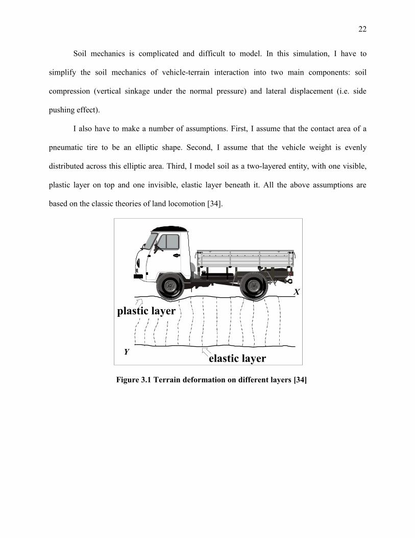
Soil mechanics is complicated and difficult to model. In this simulation, I have to

simplify the soil mechanics of vehicle-terrain interaction into two main components: soil

compression (vertical sinkage under the normal pressure) and lateral displacement (i.e. side

pushing effect).

I also have to make a number of assumptions. First, I assume that the contact area of a

pneumatic tire to be an elliptic shape. Second, I assume that the vehicle weight is evenly

distributed across this elliptic area. Third, I model soil as a two-layered entity, with one visible,

plastic layer on top and one invisible, elastic layer beneath it. All the above assumptions are

based on the classic theories of land locomotion [34].

Figure 3.1 Terrain deformation on different layers [34]

Y

X

plastic layer

elastic layer

23

Figure 3.2 Normal pressure distribution [34]

When the vehicle interacts with the soil, the plastic layer is deformed. The amount of

vertical sinkage is a function of the resistant forces from the elastic layer beneath it. The soil

elasticity is different for different types of soil or for the same soil under different climate

conditions. Figure 3.1 illustrates this process.

The lateral displacement is the result of the force at the edge of the tire-soil contact area

that pushes the top layer slightly upwards and sideways. The amount of lateral displacement,

based on the Terramechanics empirical data, is a function of the contact area and vehicle speed.

The above calculations, implemented in a vertex shader, can determine the amount of

vertical and lateral displacement of vertices in contact with the vehicle tires. However, they do

not produce distinctive tire marks. To achieve this, a displacement mapping is performed on top

of the already deformed terrain mesh.

3.3.1 Theories on Vehicle-Terrain Interaction

When vehicles run on soft terrain, the terrain is often deformed. Such deformation is due

to both vertical load V and horizontal load H. The vertical load comes from the weight of the

0.9

0.7

0.5

0.3

p0.2

p

2b

2b

24

vehicle while the horizontal load comes from the force that pushes the vehicle forward.

According to Bekker [34], the stress function for the vertical load can be represented as:

σr = - 2V

rcos (3-1)

In equation 3-1, r is the distant from the contact point to the stress point, φ is the angle of

direction of the force, and V is the vertical load (lb. per inch). For moving vehicle, I also need to

consider horizontal load H. In latter case, a force R = sloped to the vertical at angle θ

will generate stresses that can be represented by equation Bekker [34]:

σr = - 2 V2 H2

rcos (3-2)

The parameters in equation 3-2 are the same as in equation 3-1.

Figure 3.3 Vertical load V and horizontal load H [34]

The stress distribution is calculated based on vertical stress and horizontal stress. I

consider the shape of the stresses distribution under a wheel is a rectangle, and by combining

equation 3-1 and 3-2, Bekker [34] produces the solution to the stresses distribution as follows:

σx =

(3-3)

V

H

R

r

r

25

σz =

(3-4)

Where V, and r are same as in equation 3-1. 1 and 2 are explained in Figure 3.4

(reproduced from Bekker [34]).

Figure 3.4 Stresses distribution of a rectangle area [34]

For simplicity, I don’t consider forward stress σx, and use σz as the theoretical foundation

for deformation. Unfortunately, equation 3-4 is impractical in real-time rendering due to its

complexity. When adapt equation 3-4 directly to my system, it seemed to be very expensive for

the application to capture the values of and

at run time, thus leads to a low frame rate

rendering. Thus I propose a modified equation:

σz = V

a r

(3-5)

Where V, , and r are the same as in equation 3-2. I use a constant k to replacement

the value of ( -

and constant a control the value of (

-

). I find it is more

practical to use constants k and a and it gives decent appearance as well. Equation 3-5 can be

used to calculate terrain deformation on sand. Deformation on snow requires a different equation.

This is because snow is a mixture of three phases which depend on the thermodynamic

V

1

2

z

r

26

equilibrium of solid, liquid, and gaseous state instead of a simple solid state [34]. For this reason,

I treat snow as a kind of elastic material and equation 3-6 calculate the vertical stress on snow:

σz_snow =

a r m (3-6)

Where V, r are same in equation 3-1 and a, m are constants. Equation 3-6 is adapted from

the pressure function in Becker [4], which is only suitable for calculating pressure along the

center of a circular load area.

Figure 3.5 showing the comparisons of curves. Blue and green curves are my data, while

orange and red curves are experimental data from Krotkov[51]

To show that equation 3-5 and 3-6 provide accurate results, I compare the values

generated by my equations with the terrain stiffness experimental results of Krotkov [51] (Figure

3.5). They aim to develop automatic procedures to identify a variety of terrain material

properties. In Krotkov [51], they restrict their attention to two specific properties—terrain

stiffness and surface friction.

27

I compare my results with their data of terrain stiffness. From Figure 3.5, I can tell that

my deformation data on sand is close to Krotkov’s results. In addition, my data on snow is

neighbor to their curve of sawdust. Based on the results from Figure 3.5, I believe my proposed

equations 3-5 and 3-6 can provide reasonable results for calculating vertical stress on sand and

snow ground.

My terrain model contains two horizontal layers: a plastic layer on top and an elastic

layer beneath it. Under vertical pressure, the plastic layer will deform permanently. The elastic

layer, on the other hand, is treated as the traditional spring-mass model. When vertical stress is

applied onto the elastic layer, it deforms and generates force to counter-balance the pressure.

According to Wong [52], terrain can be treated as a linear elastic material and Hooke’s Law

provides theory for linear elastic material as long as the load does not exceed its limit. The

stresses functions (3-5 and 3-6) can be used to calculate how much vertical force is applied onto

the terrain.

Figure 3.6 Spring model

However, it is not appropriate to simply apply the Hooke’s Law on the terrain because it

usually does not simply behave as a perfect linear spring-mass model. The “spring constant” of

Plastic Layer

Elastic Layer

Spring

28

the terrain changes during the process of deformation. Krotkov [51] proposed a model which is

supported by parameters of lab experiments to calculate the vertical force-displacement:

x =

(3-7)

Where x is the amount of the deformation; f represents the principal stresses that do not

generate shear in the planes of their application; k and n are constants. Equation 3-7 can serve as

a general function to calculate the deformation. However, it is generally better to use a specific

function for a specific terrain material. For example, Butterfield and Georgiadis [53] proposed a

specific force-displacement for sand, soil and sawdust:

x = k loge

(3-8)

Where x and f are same as in equation 3-7; k is a constant; L0 is the asymptotic load

above which the vertical force does not increase with the displacement. Equation 3-8 is a

specific method to calculate the deformation, but its operation of logarithm requires much

amount of calculation. Simply apply it into my application causes obvious slowdown due to the

reason that this calculation occurs dozens of time per second. Based on equations 3-7 and 3-8, I

propose a modified equation for real-time simulation:

x =

(3-9)

Where f, n and k are same as in equation 3-7, and b is a constant. I apply equation 3-9 in

my simulation to calculate the depth of deformation. Note that stress f is calculated by equation

3-5 or 3-6 based on the terrain kind. Since equation 3-9 contains stress function f and a constant

specific to different types of terrains, it can adjust the depth of the deformation based on terrain

type and vehicle weight. The visual simulation results are shown in Section 5.

29

3.3.2 A Terramechanics Model for Terrain Compression

In my system, the terrain contains two horizontal layers, with a plastic layer on top and

one elastic layer beneath it. Based on the Terramechanics theory, the soil mass located in the

immediate vicinity of the contact area (called disturbed zone) does not behave elastically.

Therefore it is modeled as a sheet of plastic material. The underlying elastic layers are simulated

as the traditional spring-mass models. When pressures are applied to these elastic layers, the

springs will deform and generate forces to balance the pressure. The plastic layer will deform

along with the underlying elastic layers. Once equilibrium is reached, the deformation of the top

plastic layer becomes permanent. In my system, I use only one elastic layer for simplicity and

efficiency. Figure 3.2 illustrates the normal pressure distribution under the tires, showing lines of

equal pressure. This illustrates that, during vehicle-terrain interaction, different points on an

elastic layer receive different pressures and therefore deform for different amount, thus creating

the visual form of a vehicle track. From this illustration, I see that at a depth of 2b (the width of

the tire), the load pressure is reduced by about 50% and almost vanishes at a depth of 4b (twice

the width of the tire). Therefore the height of the elastic layer is set at 4b.

As mentioned above, I assume that the tire-terrain contact area is an elliptic shape. I

derive Equation 3-10 from Bekker’s classic terramechanics theory [34] to calculate the normal

pressure on a point within an elliptic shape.

σz = p0

(3-10)

In Equation 3-10, (x, y, z) is the coordinate of the point; p0 is the unit uniform load; r0 is

the radius of the elliptic shape; the value of p0 is the load acting upon an element of the

surface Equation 3-10 provides a good theoretical basis for calculating terrain

deformation but it is not practical for real-time simulation. Since my simulation only uses one

30

plastic layer and one elastic layer, I have developed Equation 3-11, which is based on Equation

3-10 but simplified for better performance.

σz =

(3-11)

Equation 3-11 addresses the stress distribution for a concentrated load. Specifically it

calculates the normal pressure on any given point on a horizontal elastic layer located at depth z.

The Equation 3-11 is written in polar coordinates, in which σz is the horizontal stress; and W is

the weight of the vehicle, and r = ; R is the distance from the point to the center of the

contact area; m is a variable. A soil concentration factor n is introduced to simulate different soil

types. For grass, n = 1; mud, n = 3, and for loose sands, n = 6 or n = 7. Snow often displays the

character of a plastic layer thus it needs a different treatment [34]. The results of my Equation 3-

11 (see Figure 3.7 ) fit the experimental data in Krotkov [51].

Figure 3.7 Terrain Stiffness Comparison

3.3.3 Calculating Terrain Deformation

In the previous section, I discuss the method of calculating forces applied from the

vehicle to the terrain. In this section, I discuss how to simulate terrain sinkage (deformation)

based on these forces.

31

Figure 3.8 Normal pressure on a point in soil [34]

Figure 3.9 Simulation terrain deformation with a spring-mass model

The depth of terrain deformation is a function of the external force (from the vehicle) and

terrain elasticity. Under certain circumstances, the terrain deformation can be simulated with a

traditional spring-mass model (Figure 3.9). Based on Wong [52], terrain can be seen as a

piecewise, linear elastic material, and Hooke’s Law applies to linear elastic material as long as

the load does not exceed the elastic limit. Therefore I may assume that each vertex on the terrain

model is attached to a spring. When a tire contacts a vertex, the attached spring will deform and

generate a balancing force. The amount of deformation depends on how much force is needed to

counter-balance the force from the vehicle.

32

In reality, terrain does not behave as a simple, leaner spring-mass model. The stiffness of

the terrain usually increases with the external force. As a result, the amount of terrain

deformation decreases as the external force increases. Therefore, I adopt a modified spring-mass

model for terrain deformation (Equation 3-12 . This model is based on the Krotkov’s model [51],

which is supported by lab experiments. This equation describes the relationship between normal

forces and displacement on three types of terrains: sand, soil, and sawdust.

x =

(3-12)

In Equation 3-12, f represents the normal, external force on the terrain. This force can be

calculated from Equation 3-12, depending on the terrain types. Both k and n are constants

specific to different materials; x is the amount of terrain deformation. When n = 1, Equation 3-12

is reduced to Hooke’s law.

Terrain deformation is carried out in a vertex shader in two steps. First, the terrain is

deformed with a height map of tire thread pattern. This deformation generates the base shape of

the tire tracks. Second, the depth of the base tire track is adjusted according to Equation 3-12.

3.3.4 Lateral Displacement

When an unconfined load great enough to exceed the capacity of the terrain to absorb it is

applied onto the terrain, a portion of the terrain will be displaced along the shear plane. Those

displaced parts of the soil accumulate and form the lateral and upward displacement. The sinkage

of the tire-soil contact area is due to two factors: soil compression and lateral and upward

displacement of the soil particles around the border of the contact area. The lateral displacement

is influenced by both the contact area and the duration of loadings. Experiments show that: 1. the

smaller the contact area, the stronger the effect of the lateral displacement; 2. the longer the

33

duration of loading, the stronger the effect of lateral displacement [34]. Based on the classic

terramechanic theory [34], the lateral settlement can be calculated based on Equation 3-13.

zs = σ

(3-13)

Here zs is the terrain settlement; E is the modulus of soil elasticity; h is the ground layer

thickness. However, using this equation in real-time applications is impractical. Instead, I

propose a new heuristic model Equation 3-14 to simulate the terrain settlement in a real-time

graphics program.

zs =

2n

(3-14)

Here, F is the normal force on the terrain; k is the spring constant; d is the distance from

the border of the sinkage; n is the soil concentration factor; a is a variable. Since experiments

show that within certain threshold, the smaller the loaded area, the higher the lateral settlement,

the value of a is set to different numbers for each types of terrain. This equation balances the

visual performance and the rendering cost. Even without lateral displacement, my simulation of

terrain deformation is already approaching the limit of the real-time (which is 15 fps according to

Moller [54]). Thus this relatively simple equation is critical for my simulation to render in real-

time.

When a vehicle runs on terrains such as sand or snow, the debris kicked up by the tires

will fall back onto the track. This has not been considered as part of the lateral development in

any previous works on terrain deformation. My method takes the debris into consideration.

According to the experimental results in Bekker [34], the amount of lateral displacement

is a function of vehicle loads, speed of the vehicle, and the area of the contact. In my method, the

adjusted lateral displacement y is calculated by Equation 3-15:

34

y =

(3-15)

Where comes from Equation 3-14; V is the vertical load; S is the speed of the vehicle;

c is a constant.

3.3.5 Generation of Dust Particles

The dust kicked up by a vehicle is simulated by the particle systems. The original settings

of dust include Min/Max size, Min/Max Energy, Min/Max Emission, velocity, Min Emitter

Range, Color and Local Rotation Axis and so on (see Figure 3.10). Generating dust particles

enhances the realism of the simulation.

At the beginning of the simulation, dust particles will be generated and initialized with

the original settings. Next, to dynamically create the dust, the program takes into considerations

the weight and the speed of the vehicle, which affect the amount of dust to be generated. In

addition, the speed of the vehicle affects the velocity of the dusts.

35

Figure 3.10 My settings of the dust particles in Unity3D. For snow particles, it’s similar

but different in Max Energy and Min/Max Emission

These parameters are updated each frame based on the position and the speed of the

vehicle. Dust particles are generated at the location where tires meet the ground, and deleted

after certain frames.

36

Assume that h is the height of the terrain raised by the dust particles, and I calculate h

by the following equation:

h = SA/d (3-16)

In Equation 3-16, and S are same as in Equation 3-15; A is the average value of

Min/Max Emission of dust particles at current frame; d is a constant.

3.3.6 Other Problems

As I mentioned in section 3, the simulation of terrain deformation can be divided into

four components. The above sections cover terrain deformation, lateral displacement, and dust

and debris. This section briefly discusses the simulation of tread patterns and level of detail as

well.

I use bump mapping to simulate tread patterns on the track. It is difficult to create

geometrical models of tread patterns in real time because it requires that the resolution of the

terrain mesh to be very high. Bump mapping offers a balance between the performance and the

visual appearance. My method can simulate tread patterns on both sand and snow.

I use Unity3D [9] game engine’s built-in LOD system to handle multiple levels of detail.

This LOD system also provides a solution to preserve long tracks on the ground.

3.4 Deforming by Stitching

In this section, I present a new polygon stitching algorithm based entirely on GPU. Based

on this algorithm, I propose a novel method to simulate deformable terrain, particularly the tire

tracks left on the soft terrain.

Traditional methods for deformable terrain simulation have many drawbacks. They either

use texture decal or bump mapping to fake terrain deformation, or use displacement mapping

37

techniques that often leads to excessive polygon subdivision. My method is different. Instead of

subdividing the meshes, I use a pre-created vehicle track model for the deformed terrain. During

runtime, this pre-created vehicle track mesh is sent to a geometry shader and stitched with the

existing terrain mesh behind a running vehicle. My main contribution is a polygon stitching

algorithm that takes full advantage of the geometry shader technology.

Because the vehicle track model is pre-created with a 3D modeling tool, my method can

show vehicle tracks with fine details, with a visual appearance superior to the displacement

mapping while using fewer triangles. There is no need for surface subdivision at runtime. In

addition, different tire track models can be created for different levels of details.

Although I focus on simulating vehicle tracks in this dissertation, the techniques can be

easily applied to simulate other destructible objects.

3.4.1 Previous Work on Polygon Stitching

The current work is related to polygon stitching (or polygon union) and polygons

clipping. Traditionally, polygon stitching, including terrain stitching, takes place on the CPU,

with the assumption that the polygons do not penetrate each other. For example, Martinez et al.

[55] present an algorithm for computing boolean operations on polygons, which. is an extension

of the classic plane sweep algorithm. There has been little work on polygon stitching on GPU

because, before Geometry Shader was introduced, it is impractical to conduct polygon clipping

or polygon union in shaders. The main difference between my algorithm and traditional polygon

stitching is that my algorithm is designed to take advantage of the Geometry Shader capabilities.

In addition, my algorithm handles polygons that penetrate each other. Therefore my algorithm

conducts both polygon clipping and stitching on GPU.

38

There are many applications of real-time polygon stitching, including multiple levels of

detail (LOD) and the simulation of destructible environment. In this dissertation, I focus on the

destructible environment, especially deformation terrain simulation.

More and more computer graphics applications feature destructible 3D environments.

Realistic simulation of deformable terrain is particularly important for improving the realism of

games, military training environments, or civil engineering simulators that feature many off-road

vehicles. However, simulating deformable terrain remains a major challenge, and few games

simulate terrain that can be deformed dynamically. For example, vehicle tracks in sand, snow, or

mud are rarely simulated in real time.

Existing methods for simulating deformable terrain are unsatisfactory. For examples, some

games use texture decals [56] or bump mapping to fake terrain deformation, but the realism is

lost if the camera is close to the texture.

A more advanced approach is displacement mapping, combined with dynamic LOD

[42]. The basic idea is to increase the resolution of part of the terrain mesh and then deform the

higher resolution area with a height map. The downside of this type of approach is that it is

difficult to match the subdivided polygons with the height map. If the location where the

deformation takes place does not have a lot of vertices, the visual detail is lost. As a result, these

types of methods do not display the fine tire tread patterns that I often see in the real world.

Attempting to generate such fine details would lead to excessive polygon subdivision, which is

detrimental to the real-time performance. Certain area may be over subdivided, while other areas

under subdivided. My method, which uses a pre-created tire track model and does not need

polygon subdivision, is an attempt to address this issue, while taking advantage of the Geometry

Shader capabilities.

39

More recently, some game engines feature voxel based, fully destructible 3D terrains [57,

58]. However, voxel based models are expensive to maintain and difficult to show the fine tire

tread patterns.

In [57], the author take the concept of two-dimensional height maps and show how they

could be applied to a three-dimensional space. By this way, it is easy to achieve real-time grade

simulation. A few video games have adopted the concept of volumetric environment for run time

use. This concept has been introduced for creating terrain, but it is also possible to be used for

other simulation. The use of voxels for non-terrain environment has been a core research of the

author’s game engine Thermite3D.

There are some previous work on terrain stitching, but these are CPU based approaches

and do not consider polygons that penetrate each other. For example, Zheng [59] proposed a

terrain-generation method based on the constrained conforming Delaunay triangulation, which

includes algorithms to stitch a source mesh onto a destination mesh: stenciling and stitching.

Objects such as tracks can be applied over the terrain using the "stenciling" and "stitching"

algorithms. However, either of the method deals with the actual deformation when stitching the

track onto the terrain. With few visual demonstrations, it is unclear how well these methods

perform in real time or whether it can generate visually realistic vehicle tracks.

Livny et al. [60] presented an approach to generate large scale terrain with level-of-

details. They subdivided a terrain into rectangular patches, made up of four triangular tiles

stitched with each other. But this method does not cover either deformation or polygons that

penetrate each other. My algorithm, on the other hand, handles these cases.

40

3.4.2 Polygon Stitching Algorithms

Before describing my polygon stitching algorithm, I will briefly discuss geometry shader

[61] because the entire polygon stitching process takes place in a geometry shader.

A geometry shader is a rendering stage between a vertex shader and a fragment shader. It

receives geometry data from the vertex shader, processes it – which may include removing or

emitting polygons – and then sends the geometry data to the fragment shader. In my case, the

input and output data of the geometry shader are triangles.

Since I’m interested in simulating terrain deformation, I need to deal with two kinds of

meshes: the terrain mesh and tire track mesh. Specifically, the boundary of the tire track mesh is

modeled as a quad (see Figure 3.11). Inside this quad are the smaller triangles modeling the tire

tread patterns. The terrain meshes are triangles.

The goal is to dynamically stitch the tire track mesh (a quad) with the terrain meshes

(triangles) at runtime so that tire tracks would appear behind a moving vehicle. Most

importantly, the vehicle track model needs to be seamlessly stitched (merged) with the

surrounding terrain mesh (see Figure 3.11), otherwise there will be cracks in the mesh.

41

Figure 3.11 An example of stitching a tire track mesh with a terrain mesh.

There are two main steps in stitching a tire track model with the terrain mesh. First, some

polygons on the terrain mesh need to be clipped and replaced by the tire track model, and a

geometry shader is the appropriate place to do this. This is the opposite of a typical clipping

process: the part of the terrain triangles that overlap with the tire track quad are eliminated, while

the rest of the triangle is preserved. An example is shown in Figure 3.12. TriangleABC (ΔABC)

overlaps with QuadQ1Q2Q3Q4, and the PolygonI1I2I3I4Q4I5I6 needs to be eliminated.

Second, after the clipping, new triangles are emitted through a tessellation process. In the

example shown in Figure 3.12, the new ΔCI2I3, ΔI1BI6, ΔQ4I5A, and ΔI4Q4A are emitted by the

geometry shader. Next, the new triangles, along with the tire track model and the rest of the

terrain model, are sent to the fragment shader.

[0, 1, 2][0, 1, 2]

[0, 2, 2]

[0, 2, 2]

[0, 1, 2]

[1, 1, 2]

[0, 1, 2]

[0, 2, 2]

[0, 1, 4]

[1, 0, 2] [0, 1, 2] [0, 1, 2]

[0, 2, 2]

[0, 2, 2]

[1, 1, 2]

[0, 1, 2]

[0, 1, 2]

[0, 2, 2]

[1, 1, 2]

[0, 0, 0]

42

There are two main challenges of implementing this algorithm on GPU. The first

challenge is how to send the tire track model to the geometry shader. The solution is to pass the

tire track model from the OpenGL host program to the geometry shader as a texture image. The

RGBA components of each pixel are used to store the XYZW coordinates of a vertex.

The second challenge is that a geometry shader has very limited access to the terrain mesh.

It can only handle one triangle at a time. Therefore the polygon stitching is essentially between

one quad and one triangle, and I need to identify all possible cases of clipping and tessellation.

To address this issue, I have classified 20 cases that cover all possible polygon stitching

scenarios.

3.4.3 Classification of Polygon Stitching Cases

I classify polygon stitching cases based on three criteria: 1. how many vertices of the

quad are inside the triangle? 2. How many vertices of the triangle are inside the quad? 3. How

many intersection points are there between the quad and the triangle? These tests are

implemented using the geometric algorithms discussed in [62].

For the rest of this dissertation, I will use the following notation to identify each case of

polygon stitching:

[Q, T, P]

where Q, T and P are integers and 0≤Q≤4, 0≤T≤3, 0≤P≤6.

In this notation, Q indicates how many vertices of the quad are inside the triangle, T

indicates how many vertices of triangle are inside the quad, and P indicates the number of

intersection points. For example, Figure 3.12 depicts case [1, 0, 6], in which one vertex of the

quad falls inside the triangle, zero vertex of the triangle is inside the quad and there are 6

intersection points.

43

All the possible cases are listed in Figure 3.13 and illustrated in Figure 3.14 which shows

how the merged polygons are tessellated in each case. In these figures, the dashed blue lines

represent line segments to be deleted. The dashed red lines represent line segmented to be added

to the scene. Taking Figure 3.12 as an example, the input is the TriangleABC (ΔABC) and

QuadQ1Q2Q3Q4 and the intersection points are I1, I2…… I6. Based on my algorithm, ΔABC is will

be divided into 5 parts: ΔCI2I3, ΔI4Q4A, ΔQ4I5A, ΔI1BI6, and Heptagon I1I2I3I4Q4I5I6. In the end,

the original ΔABC will be eliminated (i.e. not emitted in the geometry shader). Instead, the four

triangles and the quad mesh will be emitted, thus “stitching” the triangle with the quad.

Figure 3.12 Case [1, 0, 6]

I divide the cases into four groups: (I) all three vertices of the triangle are inside the quad;

(II) all three vertices of the triangle are outside the quad mesh; (III) one triangle vertex is inside

the quad mesh; (IV) two triangle vertices are inside the quad.

A

B

C

Q1 Q2

Q3

Q4

I1

I2 I3

I4

I5

I6

44

Figure 3.13 Four groups containing all possible cases

In group (I), since the entire triangle (terrain) is inside the quad (tire track), the triangle

must be eliminated and replaced by the quad. In other words, this terrain triangle will not be

emitted in the geometry shader.

In group (II), all three triangle vertices fall outside the quad, but the triangle may have

overlapping area with the quad. There are two special cases -- [2, 0, 4a] and [2, 0, 4b] -- that

cannot be differentiated by the notation because they have the same value for Q, T, and P but

they can be distinguished by checking if the two corners of the quad inside the triangle are

adjacent or not. Case [4, 0, 0] is unique within this group because the entire quad is inside the

triangle.

In group (III), one triangle vertex is inside the quad. Notice that cases [4, 1, P] 0 ≤ P ≤

6) do not exist.

In group (IV), two triangle vertices are inside the quad. Cases [4, 2, P], [3, 2, P] and [2,

2, P] 0 ≤ P ≤ 6 do not exist.

45

Figure 3.14 All possible cases of polygon stitching

[0, 0, 4] [0, 0, 6] [1, 0, 2]

[1, 0, 4] [1, 0, 6] [2, 0, 2]

[2, 0, 4a] [2, 0, 4b] [3, 0, 2]

[4, 0, 0] [0, 0, 0] [0, 3, 0]

[0, 1, 2] [0, 1, 4] [1, 1, 2]

[2, 1, 2] [2, 1, 4] [3, 1, 2]

[0, 2, 2] [1, 2, 2]

46

The tessellation process for groups (II), (III), (IV) can be briefly described as follows.

First calculate the intersection points between the quad and triangle, if any [62]. Second, identify

triangle vertices that are inside the quad [62]; third, identify quad vertices that are inside the

triangle [62]. Fourth, based on the above information, identify the case for polygon stitching.

Fifth, based on the rules for the specific case, emit triangles that are not overlapping with the

quad, but attached to it. Finally, after all the terrain triangles are emitted, emit the triangles

within the quad that model the tire tread pattern.

3.4.4 The Rendering Process

The Polygon Stitching Algorithm on geometry shader

// input: a triangle

Calculate the intersection points between the triangle

and quad [62];

for the current triangle

check the number of vertices in the quad [62];

for the quad

check the number of vertices in the triangle [62];

1 if triangle_vertices_in_quad = 3 // group (I)

2 case [0, 3, 0], do not emit this triangle;

3 else if triangle_vertices_in_quad = 0 // group (II)

4 if quad_vertices_in_triangle = 0

5 if num_intersection_points = 0

6 case [0, 0, 0];

47

7 else if num_intersection_points = 4;

8 case [0, 0, 4];

9 else if num_intersection_points = 6;

10 case [0, 0, 6];

11 else if quad_vertices_in_triangle = 1

12 ….. // check num_intersection_points

13 case [1, 0, 2] or [1, 0, 4] or [1, 0, 6];



16 case [2, 0, 2] or [2, 0, 4a] or [2, 0, 4b];


18 case [3, 0, 2];

19 else case [4, 0, 0];

20 else if triangle_vertices_in_quad = 1 // group (III)



23 case [0, 1, 2] or [0, 1, 4];


25 case [1, 1, 2];



28 case [2, 1, 2] or [2, 1, 4];


48

30 [3, 1, 2];

31 else if triangle_vertices_in_quad = 2 // group(IV)


33 case [0, 2, 2];

34 else [1, 2, 2];

// output: a list of triangles

Figure 3.11 shows one example of the tire track mesh stitching onto the terrain mesh.

Colored terrain triangles are clipped by the tire track quad and then tessellated. Different cases of

polygon stitching are marked in the figure.

I discussed all the cases of polygon intersection and tessellation. In this section, I will

discuss the implementation details. I implement my algorithm in OpenGL and GLSL (OpenGL

Shading language) 4.0. Specifically, the polygon stitching is performed in a geometry shader.

The terrain mesh is originally saved in an OBJ file and passed from the OpenGL program to the

vertex shader, and then to the geometry shader as a list of triangles. The vehicle tire track mesh is

stored in an image and passed from the OpenGL program to the geometry shader as a uniform

variable.

Figure 3.15 Workflow of deformable terrain simulation

Tire

Meshes

Terrain

Meshes

Terrain and

Track

Texture

Geometry Shader Fragment Shader

Stitching ProcessTexture

Mapping

Result

49

Figure 3.15 shows the procedure of my deformable terrain simulation. Initially the terrain

meshes and the pre-created track meshes are sent to GPU and then processed by my stitching

algorithm. The resulting meshes are sent to a fragment shader for texture mapping.

3.4.5 Experiment

The results of the simulation are shown in Figure 3.17, which include the rendered scenes

as well as screenshots of the wireframe mode. The resolution of the rendering window is

1200×1200. The terrain mesh contains 11900 triangles, and the pre-modeled tire track mesh has

648 triangles. This tire track mesh is seamlessly stitched with the terrain mesh at runtime. The

terrain mesh and the tire track mesh are texture mapped separately using different texture

images. On a PC with Intel Core i7 1.73GHz, 4GB memory, and NVIDIA GT425m, my program

runs at realtime performance (see Figure 3.16). In Figure 3.16, the numbers of output primitives

are different from input terrain primitives because the depths of the track left onto them are

different. More specifically, I have Depthgrass<DepthMud<DepthSand <Depthsnow.

Figure 3.16 Run time performance

50

Figure 3.17 Screenshots of my simulation in wireframe mode: (from left to right column)

grass, mud, sand and snow.

3.5 Deforming with Shaders

3.5.1 Rendering Pipeline of OpenGL

Before going to the details of my implementation, I briefly introduce the rendering

pipeline of OpenGL since my implementation takes place there.

51

Figure 3.18 OpenGL Pipeline [63]

The Rendering Pipeline is the sequence of processing stages that OpenGL takes. Two

types of graphical data, vertex-based data and pixel-based data are processed through each stage

during the rendering process. These two types of data come from the application, and can be sent

back to the application after they have gone through the pipeline [63].

The vertex data is sent to the first stage called Vertex Shader from the application. Based

on the order of the list of the vertices, points, lines or triangles will be formed. These basic

52

shapes are called primitive. Each vertex and normal coordinates are transformed by

GL_MODELVIEW matrix. This modelview matrix defines how your objects are transformed in

your world coordinate frame [63]. The vertex shader receives the attribute inputs passed from the

previous step. It then converts every incoming vertex into a single outgoing vertex based on an

arbitrary, user-defined program. The output of each vertex must have a position value filled by

vertex shader. In addition, if lighting is enabled, then lighting is calculated in this stage and then

updates the new color of this vertex.

After vertex shader stage, the primitives are sent to the optional Tessellation and

Geometry Shader. These two optional stages are called Primitive Assembly. Primitive assembly

is the process of collecting vertex data which have been processed from the vertex shader and

composing it into a viable primitive [63].

In tessellation shader, there are two sub-stages: tessellation control shader and tessellation

evaluation shader [63]. Tessellation control shader controls how much tessellation a patch gets,

while the tessellation evaluation shader takes the result and actually compute the tessellation.

The tessellation shader sits between the vertex shader and the geometry shader, and it is optional.

Figure 3.19 Geometry Shader Normal Visualizer [64]

53

The geometry shader is another optional stage in primitive assembly [63]. Unlike vertex

shader, a geometry shader can create new primitives. Geometry shader takes in a single primitive

and may output zero or more than one primitives. For each input primitive, the geometry shade

has access to all the vertices that make up the primitive, including adjacency information. The

geometry shader is the most critical part during the rendering of my application since my

application will generate new triangles during this stage.

The next a few stages in the pipeline are not programmable. In the clipping and culling

stage, the primitives are clipped and culling is done here. Clipping is the process to split the

primitives within and without viewing volume. Also, OpenGL face culling calculates the so

called signed area of the filled primitive that is in the window coordinate space and this culling

for triangles happens at this stage.

The next non-programmable stage is rasterization. Raterization converts geometric and

pixel data to fragment. A fragment is a set of rectangular array containing information about

color, depth, and line width and point size and is used to compute the final data for a pixel.

Notice that each single fragment maps to a pixel that is in the frame buffer.

The next stage fragment shader is a program which processes a fragment from the

rasterization process into a set of colors and s single depth value. It follows the stage of

rasterization. The input to the fragment shader are generated by system or passed from previous

stages. The output of the fragment shader will be a depth value, and color values to be written to

the buffers [63].

3.5.2 Implementation

Algorithm.1 describes the algorithm and process of my simulation. I implemented my

algorithm using OpenGL/GLSL on a PC with Intel core i7 Q740 1.73GHz, 4GB RAM, and

54

NVIDIA GeForce 425m GPU with 1GB RAM. The rendered scene resolution was 1200×1200

and the average frame rate is 110 frames per second. I simulate four types of terrain: grass, mud,

sand, and snow.

Figure 3.20 Illustration of the simulation process.

Algorithm.1 Creating tire tracks

1: Process mesh and textures on the CPU.

2: Send all the vertices and textures from the CPU to the GPU. Four textures are sent to the

shader: one terrain texture image (Figure 3.20-A); one height map used for track deformation;

another height map for lateral displacement; a texture image for the tire mark. (Figure 3.20-D).

3: In the vertex shader, the displacement mapping technique is used to deform the terrain. A

height map (Figure 3.20-B) is used to generate the tire tread patterns. The height values from the

height map are blended with the terrain sinkage factor, calculated based on equations to

generate the vertex displacement value.

4: The lateral settlement is added through an additional displacement mapping step, in which a

lateral displacement height map (Figure 3.20-C) is used. The height values from this height map

are then blended with the lateral settlement calculated based on equation given in the above

section. As a result, the lateral displacement is a function of tire width, vehicle load, vehicle

speed, and types of terrain.

55

5: In the fragment shader, both images of the terrain and the tire track are applied through

multi-texturing.

Figure 3.21 Simulation parameters

Figure 3.21 shows my simulation parameters, which include spring constants k and

constant n for different terrains. Note that I have mentioned that snow often displays the

character of a plastic layer. The values of constant n are based on Bekker [34]. Krotkov [51] does

not specific numbers for different spring constants k, so the numbers in Figure 3.21 are based on

my experience and testing.

The spring constants of grass and mud are relatively close. Grass has the biggest spring

constant among the four types of terrain, thus the sinkage of grass is the lowest. The snow spring

constant is based on Krotkov’s experiments on sawdust, which is close to snow in terms of

deformability. Thus snow has the smallest spring constant, and therefore tracks on snow are the

deepest, which matches the real world observation.

I use the same weight load on four types of the terrain. Each type of terrain is deformed

differently based on the soil concentration factor mentioned in section 3.

The deformation on the terrain is calculated by my model and since the spring constants

of each types of terrains are different, the depths of the tracks are different. The depth of track on

56

grass is the lowest and that of snow is the deepest. Specifically, Depthgrass<DepthMud<DepthSand

<Depthsnow. I applied Algorithm.1 in my simulation.

Using terramechanics based equations, more realistic and fast simulation has been

assured. My methods can be further applied to other types of terrains as long as the perimeters

are ready.

Figure 3.22 Screenshots of my simulation with texture mapping

57

3.6 Deforming in Unity3D

In this section, I will introduce the implementation conducted in Unity3D game engine.

3.6.1 Algorithm

My algorithm is a two-step process. In the first step, I create a “clean” impression of the

track and the lateral displacement. Then at the second step, I add a semi-random deformation to

adjust the height of the ground. It is called semi-random because the deformation is a function of

speed, weight of the vehicle and the area of contact.

1st Step:

In this first step, I deform the terrain using the theories discussed in the above section.

During this process, the vertical stress is calculated based on Equation 3-5 or 3-6 and the depth

of the deformation is calculated by Equation 3-9. In addition, the lateral displacement is roughly

generated along the sides of the tracks. The amount of the lateral displacement is calculated

based on Equation 3-11.

The deformation is implemented per vertex of the terrain, with proper bump mapping

applied.

2nd

Step:

Deformation of terrains such as sand and snow should be treated differently. On these

kinds of terrain, dust and debris will be kicked up by the vehicle running at high speed. When

these particles fall to the ground, they change the depth of the terrain deformation and the height

of the lateral displacement. Therefore in this step, I adjust the height of the terrain according to

the amount of the particles.

58

In the first step, I add the visual effect of dust particles. The amount of particles is

controlled by three parameters: speed, weight of the vehicle, and the area of contact. Since the

weight of the vehicle and the contact area are fixed, the speed of the vehicle is the most

important factor in dust simulation.

3.6.2 Rendering Algorithm

I discussed the two steps of deformation. I will show the overall algorithm of the

rendering process in this section.

Rendering Algorithm

A1: System prepares parameters for rendering

A2: When tire contacts the terrain:

//step1

Part of terrain lowers its the height

Mapping tire pattern on the ground

Edge of the track rises up to generate displacement

A3: if Speed of Vehicle > fast_speed

Position = Find(tire);

GenerateDust(Position);

DeleteDust(fixed_time);

//step2

Part of the terrain rises up

Displacement of track rises up

A4: information of heights of terrain is stored in the memory for LOD purpose

59

Parameters gathered in A1 include the weight of the vehicle, the position of the four tires,

original setting values of the dust particles. In A2, part of the terrain is deformed according to

Equation 3-9 while lateral displacement is created based on Equation 3-11. In A3, the dust will

be generated only when the vehicle moves fast enough (faster than fast_speed) and then deleted

from the scene after a while. At this part, Step 2, which has been discussed in section 4.2, is

implemented when the dusts fall onto the ground. I draw a figure to show flowchart (Figure

3.23).

Figure 3.23 Flowchart of my simulation

h

1st Step

2nd

Step

we deform the terrain

using the theories

discussed in section 3

we adjust the height of the

terrain according to the

amount of the particles

original status of terrain

before the simulation starts

terrain height from

1st step

terrain height after

2nd step

dust

60

3.6.3 Analysis and Result

I render my application in two kinds of terrains: sand and snow.

For both types of terrain, I set the height map size to 2000×2000. The terrain model is a

two-dimensional rectilinear grid. The tile size of the terrain texture is 15×15, while that of the

track pattern is 10×10. The rendering statistics can be found in Figure 3.24.

Figure 3.24 Rendering Statistics

In Figure 3.24, Triangles and Vertexes mean the numbers of triangles and vertexes drawn

in the scene; Used Textures means the number of textures used to draw this frame and their

memory usage; Animation means the number of animations playing in the scene; VRAM usage

means approximate bounds of current video memory (VRAM) usage; VBO total means the

number of unique meshes (Vertex Buffers Objects or VBOs) that are uploaded to the graphics

card. These values were collected by Unity3D built-in statistics window during run-time of the

application.

Figure 3.25 shows the simulation on sand. The simulation starts with an off-road vehicle

starting to run on the sand ground, with dusts kicked up into the air. The first row of the

screenshots shows the start of the simulation; the second row shows the terrain deformation

61

made by the tire; the third row shows the vehicle running with the dust kicked up into the air.

More screenshots are showed below.

Figure 3.25 Simulation on sand

62

Figure 3.26 more screenshots of simulation on sand

63

Figure 3.27 Simulation on snow

Figure 3.27 shows screenshots of simulation on snow. It shows a running vehicle leaving

a track on snow. More screenshots of snow terrain are showed below.

64

Figure 3.28 more screenshots of simulation on snow

65

4. SHIP OSCILLATIONS

4.1 Ship Oscillation Problem Statement

Ship motion is an important part of water based visual simulation. The most interesting

ship motions are the ship oscillations as wave after wave acting upon the hull. In ship motion

terms, waves cause the ship to roll, pitch, yaw, heave, sway, and surge. Previous works have not

addressed ship motion effectively since most of the previous works are concerned with

simulating realistic waves or fluid dynamics [65-67]. Some methods have been developed for

simulating solids floating on water [68, 69]. These works often treat the solid as discretized

object and apply physics calculation on a node by node base. Although the physics simulation is

more accurate, it is not suitable for real time applications. Besides, these methods are not

specifically developed for simulating ship motion.

My method treats ship as a whole and calculates ship oscillations based on the forces

generated by waves. The method is based on the physics theories of ship motion, but I made

necessary simplifications for real time applications. As a result, my method can simulate realistic

ship oscillation in reaction to waves with different directions, frequencies and amplitudes. More

importantly, my method runs in real time and therefore is suitable for applications such as

games, trainings, and visual simulations.

Compared with previous works, my method is more narrowly designed for simulating

ship motion, but it is much more efficient and can present physically realistic ship oscillations. In

addition, my method can detect whether a ship will capsize in a particular wave, which is useful

for ship and cargo load animation.

66

4.2 Previous Work of Ship Oscillations

To simulate the dynamic behaviors of a floating solid, it’s important to study the

interaction between fluids and solid, especially the effects fluid has on the floating object. There

are a lot of research on simulating the interaction between fluid and solid [65-74].

In terms of coupling direction, fluid-solid coupling can be divided into three categories:

one-way solid-to-fluid coupling, one-way fluid-to-solid coupling and two-way coupling [70].

The first type of one direction coupling, solid-to-fluid coupling, considers the motion of the rigid

body as predetermined and the motion of the fluid is affected by the rigid body. One popular

example would be a ball splashing into a pool of liquid [65-67]. Foster [65] introduced an

algorithm to build on a technique for calculating three dimensional fluid flow. Their algorithm

can be applied as a general tool for animating liquids. The major contribution of their work is

that for the first time, animators become possible to create and control a 3D fluid animation

without understanding complex theories, equations. Their algorithm provides stable and effective

way to be used with general animation technique. They have showed examples of moving

objects and explosions to demo the effectiveness of the proposed algorithm.

Foster [66] also presented a method for modeling liquids and the result is a technique that

is very general for specifying how the liquid should behave.

Enright et al. [67] present a new method for the animation and rendering of photorealistic

water effects. They have focused on the simulation of 3D effects such as pouring of water into a

glass and the breaking of an ocean wave. They have used a newly proposed algorithm to

simulate the water surface as realistic as possible, and this new algorithm is a front tracking

manner. The velocity plays an important role in their simulation. They are able to gain control to

67

the surface motion due to the velocity extrapolation method. An advanced physically based

rendering system has been adopted to ensure the decent final images of rendering.

On the contrary, the other type of one direction coupling, one-way fluid-to-solid coupling

simulates how fluid affects the motion of rigid bodies without being affected by the rigid bodies.

For example, Chen and Lobo [68] simulated objects drifting on fluid as streak-line particles.

They have introduced a way for physically based modeling and real time simulation of 3D fluids.

They were able to map the surface into 3D by utilizing the pressures in the fluid flow field. Their

work is advanced over the previous work because their work could simulate many different fluid

behaviors by modifying the internal or external boundary parameters. They stated that their

model could simulate different kinds of fluids by varying the Reynolds number [75]. In addition,

their work could be used to simulate other floating objects. Their model can serve as a test-bed to

simulate a few fluid phenomena which have not been worked on before.

Foster and Metaxas [69] animated solid object (e.g. tin cans) floating on water. They

assumed the solid object is discretized and consists of a set of nodes, and the force applied on

each node is calculated according to the pressure and velocity of the fluid. They have introduced

a novel algorithm to render the animation of liquid phenomena. They have studied previous

methods of simulating fluids and also add more complex behavior to the simulation. Their

methods are based on the Navier-Stokes equations. Their simulation scene is an environment

which contains an arbitrary distribution of fluids. In addition, there are floating object on the

fluids. In their simulation, velocity and pressure of the fluids play important roles. The coupling

between obstacles makes it possible for the simulation of a number of different types of effect.

These are the main contribution of their work.

68

In two-way coupling [70-74], the solid object and the fluid influence each other’s motion.

Typically the coupling of fluid and solid is to set the velocity of the solid as boundary condition

for the fluid, and use the fluid pressure as the boundary condition for the solid. For example,

Genevaux et al. [72] represented the solid with a set of linked point mass. Taking all the forces

into account, they calculate the overall force applied to each point and update its position

independently. Their method relies heavily on the definition of a coupling force between the

solids and the fluid. However, their method doesn’t conserve the torque and therefore couldn’t

handle the rotation of the solid effectively.

Carlson et al. [70] treated the solid as fluid and the motion of the solid is simulated as that

of fluid at first. Later on, they enforced the rigidity by using a Lagrange multiplier. Their method

is a rigid fluid method since the simulator regards the rigid objects as if they were fluid. The

implementation of their method is straightforward and can be added to current fluid simulator.

Batty et al. [71] approximated a J operator to map the pressure of fluid to torque on the

solid. However the mass matrix they used to approximate the volume weights is not consistent

with those volumes. That becomes an issue when simulating buoyant solid in hydrostatic rest as

indicated by the authors in the paper.

In my work, I focus on simulating ship motion, particularly ship oscillation. Ship

oscillation in waves can be considered a special case of one-way fluid-to-solid coupling.

However, none of the previous fluid-to-solid and two way coupling methods has dealt with ship

motion specifically. It may be argued that some of the previous methods are general enough to

handle ship motion. But with the size and complex shape of a ship, it will be difficult to simulate

ship motion in real time with the existing methods that treat 3D objects as discretized entities. In

fact, there is a more efficient and physically realistic method to simulate ship motion. In this

69

dissertation, I am exploring this method. Instead of treating ship as a discretized object and

calculate forces per node, my method calculates the forces applied to the entire ship based on the

theory of ship motion [76]. In other words, most previous methods are based on general physics

theory while my method is based on the more specialized ship motion theory. As a result, my

method is more efficient and realistic for simulating ship motion.

4.3 Ship Algorithms

In this section, I describe my method to simulate realistic ship motions in various waves.

My method is based on the physics theories of ship motion but with necessary simplifications for

real time simulations. My method assumes that the fluid is incompressible and the gravity is

constant. It also disregards the viscous effect and assumes that the ship has zero forward speed

with arbitrary heading. This is because the underlying ship motion theories are also based on the

same assumptions.

4.3.1 General Ship Oscillation Model

Ship motions are caused by multiple forces acting upon the hull. The total force on a ship

is a linear combination of hydrostatic forces and hydrodynamic forces. Hydrostatic forces are

restoring forces due to gravity and buoyancy. Hydrodynamic forces include first-order wave

excitation forces, second-order wave excitation forces, radiation forces, and viscous forces. Here

I ignore second-order wave excitation forces and viscous forces due to their complexity of

calculation and also because they are insignificant compared to other components.

First-order wave excitation forces can be further divided into Froude-Krylov forces and

diffraction forces. Radiation forces can be divided into added-mass forces (with is proportional

to wave accelerations) and damping forces (which is proportional to wave velocities).

70

Figure 4.1 The six degrees of freedom of a ship

Wave excitation forces cause a ship to oscillate in six degrees of freedom [76]: 1, surge;

2, sway; 3, heave; 4, roll; 5, pitch and 6, yaw (Figure 4.1). More specifically, let (X, Y, Z) be a

right-handed coordinate system aligned with the center of the ship, with Z axis pointing upward.

The surge, sway, and heave are the translatory displacements along X, Y and Z axes; the roll,

pitch, and yaw are rotations along X, Y, and Z axes.

Based on ship motion theories [77], the total force acting on the wetted surface of the

ship is given by:

F= ( - ρg

+ ρg ) + (ρ

j

0 2

+

(ρAsin (4-1)

Where ρ is the density of the fluid; g is the gravity; n is the normal of the ship surface; S

is the area of wetted surface; ω is the wave frequency; is the submergence under unperturbed

surface and 0 is the free surface elevation; 0

j is oscillation amplitudes, where j ranges from 1 to

6, representing six degrees of freedom; A is wave amplitude; j and A are radiation potential

and diffraction potential; t is the instance of time.

Z

YX surge

sway

heave

yaw

roll

pitch

71

In Equation 4-1, the first term represents the hydrostatic component. The second term is

the radiation force, which is comprised of added-mass and damping forces. The third term is the

first-order wave exciting force, which is the sum of Froude-Krylov force and diffraction force.

Froude-Krylov force FFK is determined by the integration of wave induced pressure as if the ship

is fully transparent for incident waves. In Equation 4-1, radiation and first-order wave exciting

forces can be calculated based on the potential flow theories [77], but it is impractical to

implement it in real time applications. To simplify the calculation, I assume that the ship is a

symmetric object with a slender hull, and a random incident wave can be decomposed into a

combination of head waves and transverse waves. Both assumptions are reasonable as they are

adopted in ship motion theories [76]. As a result, Equation 4-1 can be replaced by simplified

equations Equation 4-2 and Equation 4-7.

A random incident wave can be decomposed into head waves and transverse waves.

Therefore, I calculate ship transformations based on the forces generated by the head waves and

transverse waves. The combined transformations produce the ship oscillations in the random

incident wave.

4.3.2 Simulating Ship Motions in Head Waves

This section considers the force generated by the head waves. Head waves move in the

opposite direction of the ship. Head waves cause the ship to pitch around the Y axis and heave

around the Z axis.

The force from small head waves acting on the ship FHead can be calculated by the

following equation [77]:

FHead = ρg - H2 ρ

coskη dη sin +

(4-2)

72

Where ρ, g, and t are the same parameters as in Equation 4-1. AH and ωH are head wave

amplitude and frequency, respectively; L is the length of the hull; η is the distance from the force

acting point to the midship; a and k are constants. B33 and A33 are damping and added-mass

coefficients in heave, respectively. Generally, Bij is the damping coefficient in the i-th direction

when the ship oscillates in j-th motion, where i and j range from 1 to 6, representing the six

degrees of freedom. Damping coefficient is proportional to the wave velocity. Aij is an added-

mass coefficient, which is proportional to wave acceleration. The damping coefficient Bij and

added-mass Aij can be computed by:

Bij = ρg

H3

j0

2L/2

-L/2dL (4-3)

Aij = b Bij (4-4)

Where ρ, g, and ζ0

j are the same as those in Equation 4-1 and AH and ωH are same as in

Equation 4-2. L is the length of hull. For fast computation, the value of Aij is calculated by

Equation 4-4 where b is a constant. Similar to Equation 4-1, Equation 4-2 is comprised of the

hydrostatic restoring force, the Froude-Krylov force and the radiation force. I neglect the

diffraction force since it is insignificant compared with the Froude-Krylov force. Solving

Equation 4-2, Equation 4-3 and Equation 4-4, and I can calculate the amplitude of pitch

oscillation α, and heave oscillations β, as follows:

α =

ρg

H

2 ρg

H

2 (4-5)

β =

ρg

H

2 ρg

H

2 (4-6)

Where m is the mass of the ship and B55 and A55 are damping and added-mass

coefficients in pitch. B33 and A33 are damping and added-mass coefficients in heave.

73

4.3.3 Simulating Ship Motions in Transverse Waves

This section considers the forces generated by transverse waves. Transverse waves move

perpendicularly toward the hull of the ship. Transverse waves cause the ship to roll around the X

axis and heave along the Z axis. According to ship motion theories [77], the force generated by

transverse waves acting along the ship’s hull can be calculated by the following equation:

FTransverse = (ρgAwp - T2 )AT sin + AT cos (4-7)

Where ρ, g and t are the same as those in Equation 4-1 and Awp is the water-plane area;

AT and ωT are transverse wave amplitude and frequency, respectively. A33 and B33 are added-

mass coefficients and damping coefficients, respectively (see Equation 4-3 and Equation 4-4).

The total force in Equation 4-7 is the linear combination of Froude-Krylov force and the added-

mass and damping forces. Solving Equation 4-7, Equation 4-3 and Equation 4-4, then I can

calculate the amplitude of roll oscillation γ and heave oscillation δ as follows:

γ =

g

2 g

2 (4-8)

δ =

g

2 g

2 (4-9)

Where m is the mass of the ship, B44 and A44 are damping and added-mass coefficients in

roll and B33 and A33 are damping and added-mass coefficients in heave (see Equation 4-3 and

Equation 4-4). The results obtained from Equation 4-8 and Equation 4-9 determine how the ship

rolls and heaves in transverse waves.

The transverse wave-induced force causes the ship to roll around X axis, while the

hydrostatic force tries to restore the ship to its rest position. If the rolling angle θ >= 72 degree

[76] around the X axis, the ship will capsize. Therefore, to keep the ship afloat, the hydrostatic

restoring force FR should be proportional to θ: FR = θ FTransverse/72. The interactions between

74

transverse wave-induced force and hydrostatic restoring force produce the lateral ship

oscillations.

4.3.4 Simulating Ship Motions in Random Incident Waves

A random incident wave can be decomposed into a linear combination of a head wave

and a transverse wave. This process can be regarded as multiple layers of wave combined to

represent the random incident wave (Figure 4.2), and is generally accepted in shop motion

theories. Therefore, the ship motions in random incident waves can be simulated by combining

the oscillations caused by the decomposed transverse waves and head waves. For simplicity, in

this method a random wave is decomposed on the horizontal X-Y plane.

Figure 4.2 Incident wave

A random incident wave is identified by its frequency ωArbitrary and amplitude AArbitrary. In

order to calculate forces based on Equation 4-2 and Equation 4-7, I decompose the frequency and

amplitude of a random incident wave to a transverse wave component and head wave

component. Assume that the angle between an arbitrary incident wave and the ship is α, then the

frequencies and amplitudes of head and transverse waves ωH, ωT, AH and AT can be calculated

by:

ωH = ωArbitrary · cos α, ωT = ωArbitrary · sin α (4-10)

AH = AArbitrary · cos α, AT = AArbitrary · sin α (4-11)

75

By feeding ωH, ωT, AH and AT into Equation 4-2 and Equation 4-7, I can proceed to

calculate the amplitude of pitch, roll, and heave. More details will be discussed in the next

section.

4.4 Ship Oscillation Implementation

In this section, I discuss my implementation and show the rendering results obtained from

my simulation. My simulation is rendered in real time with an average frame rate of 46 fps at a

resolution of 1280×720. The simulation is built with the Unity3D game engine [9] on a PC with

Intel core i7 Q7401.73GHz, 4GB RAM, and NVIDIA GeForce 425m GPU with 1GB RAM.

The waves in my simulation are modeled by combining multiple sinusoids. Each wave is

defined by its frequency, amplitude, and direction. My simulated environment is an ocean, which

has a large scope and no boundary. In addition to the waves and ship motions, other visual

effects, such as reflection and refraction are implemented as well.

Rendering Process

1: First, the values of the parameters in Equation 4-2 to Equation 4-11 are specified. A sample

of the main parameters is shown in Figure 4.3.

2: The system automatically generates random waves. Each wave is decomposed into a head

wave and a transverse wave.

3: Calculate the forces induced by the head waves and transverse waves, and then calculate the

amplitude of pitch, roll, and heave. The calculation of surge, sway, and yaw are simplified for

performance. Specifically, the amplitude of surge is a simple linear function of the amplitude of

pitch. The amplitude of sway is a linear function of the amplitude of roll. The amplitude of yaw is

also a linear function of the amplitude of roll. All the transformations are applied to the mass

center of the ship to produce ship oscillation.

76

4: Repeat steps 2 to 3 to simulate continuous ship oscillations. .

Figure 4.3 Simulation Parameters and Results

Figure 4.4 Screenshots of ship oscillation in head waves

77

Figure 4.4 shows a cycle of ship oscillation in head waves, where the ship first heaved

and pitched (Figure 4.4-1 to Figure 4.4-4) due to the head wave and then was restored (Figure

4.4-5 to Figure 4.4-6) hydrostatic forces. The force generated by the head wave causes the ship

to pitch and heave.

Figure 4.5 Screenshots of ship oscillation in transverse waves

Figure 4.5 illustrates a cycle of ship oscillation caused by transverse waves. The ship was

in the buoyant equilibrium at the beginning of the simulation. Once transverse waves act on the

hull, it begins to roll and heave. Hydrostatic forces then try to restore the ship to its initial

position. Figure 4.6 shows the ship oscillations in random waves.

Figure 4.6 Screen Shots of Ship Oscillations in Random Waves

78

5. VIRTUAL URBAN ENVIRONMENT

In this section, I describe the design and development of a virtual environment for

evaluating the effectiveness of a mobile application that helps prevent pedestrian accidents when

crossing streets. Pedestrian safety is a serious concern in urban environments, and most accidents

happen when pedestrians are crossing streets. Recent studies have shown that increased mobile

phone use among pedestrians leads to increased distraction and unsafe behavior. To address this

issue, I have developed a mobile phone application that alerts pedestrians before they cross

potentially dangerous streets. To evaluate the effectiveness of this application, I developed a

virtual environment (VE) to simulate the urban environment around my university campus. I

recruited a group of students to test the mobile application in the VE by having them virtually

walking on the street while talking on the phone. The motion of the virtual pedestrians in the VE

were recorded by the program and analyzed to study the pedestrian behavior with and without

the safety alert application. I want to know whether the safety alert mobile application could

increase the pedestrian’s awareness and reduce the risky behavior when the pedestrian is

crossing a potentially dangerous street. The results show that this VE provides an efficient,

flexible, and well controlled environment for public health and geosciences researchers to test

their hypotheses and explore alternative solutions. Although the VE cannot replace the real world

field testing, the flexibility to manipulate and control the virtual environment and the ability to

monitor the pedestrian behavior in real-time prove to be a powerful feature.

5.1 Introduction

Pedestrian injury is a leading cause of pedestrian mortality, especially in urban

environments. National Highway Traffic Safety Administration (NHTSA) estimates that 4,600 to

5,300 pedestrians are killed by motorists, and 80,000 to 120,000 more are injured each year [78,

79

79]. The estimated annual economic impact is nearly $29 billion. Most of the pedestrian traffic

accidents happen when pedestrians are crossing the street. Recent studies have shown that

increased mobile phone use among pedestrians leads to increased distraction and unsafe behavior

during street [80-89]. For example, Bungum et al. [82] found that distracted walkers used less

cautionary behavior, such as looking left and right, waiting for a walking signal before crossing

streets. A study by Stavirnos et al. [83, 84] found that “cell phone conversations distracted

college pedestrians considerably across all pedestrian safety variables measured, with just one

exception.”

To address this issue, I have developed a mobile phone application that alerts pedestrians

before they cross potentially dangerous streets. The focus of this dissertation is on the evaluation

of this mobile phone application in a virtual environment. I want to study how the mobile

application affects pedestrians’ street crossing behavior and whether it reduces the risky

behavior.

The ideal method to test this pedestrian safety mobile application to conduct field studies

in the real world, which I plan to do in the near future. However there are significant difficulties

for conducting such tests in real world. Real world is an uncontrolled environment, where

pedestrian behavior is influenced by many factors. The car traffic and the pedestrians’ traffic

surrounding the test subject is different from subject to subject. It is also difficult to observe and

measure the subjects’ behavior in the real world.

My solution is to build a virtual urban environment to evaluate this application. This

virtual environment contains the roads, buildings, and traffics of an urban environment and

serves as an experimental “sandbox”. It can automatically collect the user behavior in this virtual

environment. Unlike the real world that is consisted of various distractions, the virtual

80

environment is a controlled environment that researchers can configure according to their

interests. For example, in a virtual environment, I can adjust the traffic pattern or road conditions

to test different hypothesis.

I conducted a number of experiments in the virtual environment, and the experiments in

the virtual environment show that my mobile pedestrian safety application has significant and

positive effects on the pedestrian behavior. For example, with the safety alerts turned on, the

pedestrians waited longer before crossing the street and looked around more.

There have been a number of studies that used virtual environment to study pedestrian

behavior or teach pedestrian safety [90-92]. However, my work focuses on studying the

effectiveness of a mobile pedestrian safety application. In addition, I make extensive use of

realistic 3D city models from Google Warehouse. My work shows that it is possible to quickly

build a virtual environment that resembles a real urban environment, and it is an effective tool

for testing new ideas before field testing in the real world.

This section is organized as follows. In chapter 5.2, I discuss related work. In chapter 5.3,

I describe the development of my mobile application and also the major components of my

virtual environment. In chapter 5.4, I discuss a user study conducted in this virtual environment

and the evaluation of the mobile application based on the analysis of user study results.

5.2 Related Work

Some of the pedestrian safety studies were done in virtual environments. For example,

Simpson, et al. [93] and Pandey, et al. [86] used a VR tool to investigate road crossing behaviors

in children and young adults. McComas, et al. [90] demonstrated the effective of a virtual

environment in teaching pedestrian safety to children. Schwebel and McClure [91] studied four

groups of 60 children in various settings and showed that VE is effective in training street

81

crossing skills. Schwebel, et al. [92] studied a group of 102 children and 72 adults and found that

their behavior in the virtual environment correlated with that in the real world.

Some researchers have used VEs to teach safe street crossing behavior. Katz, et al. [94]

used a VE to train patients with right hemisphere stroke for safe street crossing. Similarly, Bart,

et al. [87] builds a VR tool to teach children how to cross streets safely.

My virtual environment is different from the previous works in several areas. First, I

attempt to replicate real urban environment by using 3D building models from Google

Warehouse and use Google Map to place the 3D building models and roads. This allows us to

build relatively large scale and realistic virtual urban environment in a short period of time.

Previous virtual environments in pedestrian safety studies, however, are much smaller and

simpler. Second, the purpose of building my virtual urban environment is to evaluate the

effectiveness of a mobile pedestrian safety application, while in previous studies that involve VE,

the purpose is to either observe the pedestrian behavior or teach the safe street crossing behavior.

My virtual environment is linked with a mobile Android application and the simulation is based

on the real accident data. My virtual environment contains a mixture of virtual and real data.

5.3 Design of the Virtual Environment

5.3.1 Mobile Pedestrian Safety Application

To help reduce the risk of pedestrian accidents, I have developed a mobile application for

pedestrian accident prevention. The goal is to alert the pedestrian about the potential danger

when he or she is about to cross the street. This system consists of two main components: a web

based program for monitoring the pedestrian location and motion, and an online database that

stores the geocoded pedestrian accident data. The web based program runs on the mobile phone

and uses JavaScript, Google Maps API, and Google Web Toolkit SDK to monitor the GPS

82

locations of the pedestrian. It also monitors the pedestrian’s walking speed. The web program

would periodically contact an online database to determine whether a pedestrian is getting close

to an intersection. If so, then a risk factor is calculated based on the previous pedestrian accidents

in the surrounding area, the walking speed of the pedestrian, and other factors. An alert is

generated on the mobile phone based on the risk factor. The alert can be a beeping sound or a

vibration.

Figure 5.1 Each red point indicates that accident has occurred at that intersection.

The web based program works on both iPhone and Android phones. The online database,

which contains the pedestrian accident data and geolocations of the intersections (Figure 5.1) is

stored in a Google Fusion Table. The pedestrian accident data is obtained from the state

department of transportation. The data contains the geolocation, date, local speed limit,

pedestrians’ ages and other information related to the accidents.

83

I am interested in studying the impact of this application on pedestrian behavior and

whether it induces safer road crossing behavior, such as slowing down, waiting, and looking left

and right. Before conducting extensive field tests, I would like to test my hypothesis in a

controlled virtual environment, which will be discussed in the next section.

5.3.2 Virtual Environment

I have created a 3D virtual environment that replicates my university campus (Figure

5.2), which is located in the center of a big city. I choose to build this environment because my

test subjects are familiar with it. In the future, I will gradually expand my virtual environment to

include other parts of the city.

Figure 5.2 Screenshot of my virtual environment

I use the game engine Unity 3D [9] to develop the virtual environment. Unity 3D is a

popular, award winning game engine that allows the users to edit the game environment in a GUI

84

and write scripts to animate and control the game entity. The main components of the virtual

environment are buildings, roads, traffic, and first-person avatar.

The majority of the 3D building models are built by Google Building Maker and the rest

are imported from Google 3D Warehouse, which contains most of the buildings in major cities.

After the 3D models are created, they are exported to Google SketchUp for further editing and

then exported to Unity 3D. The terrain and the trees are created with Unity’s built-in terrain

manager. The buildings and streets are placed in the virtual environment based on Google Maps

in order to ensure accurate building size and location. My VE has 19 intersections and all the

roads were built as two-way roads. There are sidewalks on both sides of the road.

Tools like Google 3D Warehouse, Google SketchUp, Google Maps, and Unity make it is

possible to quickly build a realistic virtual environment. The end result is a virtual environment

that closely resembles my campus. The users often commented that the familiar and realistic 3D

building models enhance the immersiveness of the virtual environment and give them strong

location awareness.

I developed a traffic engine to simulate urban road traffic, using Unity’s built-in script.

Vehicles are constantly fed into the virtual environment and then recycled. Traffic rules are

implemented for the cars, but occasional traffic violations are simulated. The density of the

traffic can be adjusted to simulate different traffic patterns. Car noises are attached to the

vehicles, and background noises are placed throughout the virtual environment. All the sound

effects are 3D positional sounds.

The virtual environment is projected onto a visualization wall with 4 x 3 30’’panels each

with 2560 × 1600 resolution (Figure 5.3). The specifications of the computer are four Intel Quad

Core i7 processor systems each with 12GB high-speed memory and 6 Graphics Processing Units.

85

The virtual environment is seen from a pedestrian’s first person viewpoint. By default, the avatar

moves forward at a steady speed by itself. The user can change its direction by pressing A (left)

and D (right) keys, slow down or stop the avatar by pressing S key, or rotate the camera with

mouse motion to look around. The actions that the tester can perform in the virtual environment

include walking, stopping, jumping, and viewing.

Figure 5.3 Pictures of the VE on a large curved visualization wall

5.3.3 User Study Design

I conducted a user study to evaluate the impact of the mobile pedestrian safety

application on pedestrian behavior in the virtual environment. I recruited 24 college students, and

divided them randomly into four groups. Each subject is asked to control the avatar to follow the

same route to a destination and then “walk” aback to the starting point. The avatar can be hit by

vehicles, so the subject has to be careful. In the process, the avatar will have to cross eight

intersections. Figure 5.4 shows the main components of the system. One of the four groups

86

would talk on the cell phone while “walking” in the virtual environment until they reach the

destination. The subjects in the second group would be text messaging while walking. The VE

will trigger an alert on the subject’s cell phone when they approach a potentially dangerous

intersection. The subjects in the third group would be talking on the phone, but without any alert.

The fourth group would be text messaging without any alert.

During the test, a research assistant would ask or text the subjects over the phone based on

a pre-prepared list of questions to distract the subjects. Each subject is asked the same set of

questions. A sample of the questions is as follows.

What classes do you take this semester?

Which of them is your favorite?

When do you plan to graduate?

What is the zip code of your home address?

What do you want to eat for dinner today?

What movie did you watch recently?

What genre of music do you like?

Figure 5.4 Main components of the system, which is a mixture of virtual environment

and mobile application.

87

5.4 Results and Analysis

5.4.1 Data Collection

I wrote a script to record the current time and location of the avatar in the virtual

environment every two seconds. This information is used to calculate the waiting duration before

a subject crosses a street. In addition, the number of head turns was recorded. Figure 5.5 and

Figure 5.6 show the waiting duration and the number of head turns for all 4 groups and 7

intersections on average. Group #1 are the subjects who were talking on the phone with the alert

on; Group #2 are the subjects talking on the phone without alert; Group #3 are the subjects who

were text messaging with the alert on; Group #4 are the testers who were text messaging without

the alert on. Each group contains 6 subjects and each trial contains 7 intersections.

Figure 5.5 A comparison of waiting time among subject groups. The horizontal axis is

the subject number.

88

From Figure 5.5, I can see that on average, Group #1 spent more time on crossing the

street than Group #2. During the experiment, subjects in Group #1 tended to stop talking on the

phone immediately when they heard the alert on their phone. They stopped to look around even

if it’s in the middle of the conversation.

Figure 5.6 A comparison of head turns (looking around) among subject groups. The

horizontal axis is the subject number.

From Figure 5.6, I observed that subjects in Group #1 looked left or right more than Group

#2 did. Results from Group # 3 and Group #4 are similar. It took longer for Group #3 to cross

each intersection than Group #4. Subjects in Group #3 stopped text-messaging when the alerts

were triggered and they look around more than Group #4. Some subjects were distracted by the

89

text-messaging and did not watch out for the traffic until they heard the alert. Interestingly, this

type of subjects usually paid more attention to the traffic once they were alerted. Another

observation is that Group #3 was the “slowest” group and they looked around the most among

the four groups.

5.4.2 Data Analysis

Figure 5.7 Mean, variance and standard deviation of the results

The results show that the mobile pedestrian safety application has positive impact on

pedestrians’ street crossing behavior. Group #1 and Group #3 (with alerts) waited longer on each

intersection before crossing. Moreover, they tended to be more cautious as they looked left or

right more. Figure 5.7 shows the mean, variance and standard deviation of the results.

Among all four groups, Group #3 is the most cautious. When comparing Group #3 and #4,

I noticed that Group #3 waited longer and looked around more. All the experiments were

conducted under very similar conditions and the only difference between those two groups was

90

the alert, thus the behavioral differences can be attributed to the mobile phone application. In

Group #3, 65% of the subjects claimed that when they were texting in real life or in VE, it was

easy to get distracted by the texting and neglect the traffic. This is consistent with the results by

Schwebel et al. [86].

Since both Group #1 and #3 had the pedestrian safety application running on the smart

phone during the experiments, the difference of the waiting time might be caused by the different

cognitive complexity of phone conversation and texting. Subjects in group #1 can still look at

the traffic while talking. On the other hand, Group #3 is more distracted by the texting.

The results are submitted to ANOVA, which I use to statistically analyze the results in

Figure 5.7. The effect of distractions was observed for the Waiting Duration, F (3, 44) = 6.362, p

= 0.001, which is enough to reject the null hypothesis. When comparing Group #1 and Group #2,

I found that the alerts have a significant effect on the behavior difference: F (1, 22) = 7.653, p =

0.011. Same conclusion can be drawn from analyzing the results between Group #3 and Group

#4: F (1, 22) = 13.714, p = 0.001, which indicate a even more significant effect of the alert.

I have analyzed the mean (average) and the standard deviation of the Head Turns in

Figure 5.7 using ANOVA method as well. The results also show that the alert had a significant

effect on the pedestrians’ behavior. I observed F (3, 44) = 4.921, p = 0.005 when comparing the

number of head turns in all four groups. Also I observed F (1, 22) = 4.408, p = 0.047 when only

Group #1 and Group #2 are considered.

This indicates that the application had a significant effect on the participants when they

were at the intersections. When comparing the head turns of Group #3 and Group #4, I have F (3,

44 = 10.452, p = 0.004, which indicates an even greater effect of the alerts on the participants’

behavior.

91

5.4.3 User Feedback

I gathered user feedback after each trial was finished and I have got some useful and

heuristic information. First of all, my simulation environment (campus wide) was highly

evaluated by most of the testers (87.5%) since it greatly restores the campus surroundings. These

comments are meaningful to us since the range of my accident data is my campus and familiar

environment brings greater awareness to the testers. Secondly, I was enlightened to expend my

smart phone allocation to be used by not only pedestrians but also drivers who are driving in the

city area. Driver who has an alert-based phone could be warned when he/she is approaching an

intersection where many accidents occurred before. By that way, it may be possible to further

prevent pedestrian-vehicle accident from happening.

6. FUTURE WORK

Based on my current work on real-time simulation on terrain deformation and ship

oscillations, I plan to conduct my near future research on the following aspects.

6.1 Future Research Directions

I. Moving Ship Oscillation:

Up to today, my research on the simulation of ship oscillation is based on the pre-

requirement that the ship has zero forward speed. When the ship is in this status, the

counter-forces generated by the interaction of ship and the water can be neglected.

However, moving ship or other objects are even common in the real world. Thus I

plan to integrate forward speed into the simulation model. When the forward speed is

taken into consideration, the counter-forces generated by the interaction between the

hull of the ship and the water plays an important role of how the ship oscillates. As

92

stated, many researchers are not focusing on the behavior of the floating but the

visual effect of the water.

I plan to bring hydrodynamic theories to the simulation to solve the problem. The

problem I’m facing right now is the theories are too complicated for fast rendering.

The way to go should be simplifying without comprising the visual effects.

II. Adding Irregular Waves:

The water waves in my current research are called regular waves, whose amplitudes

are same in heights. Even though I don’t work on the visual effect of the water, the

value of the wave amplitudes is still a major factor when simulating the behavior of

the ship.

When a wave is not regular wave, the right way to simulate it is to superimpose a few

regular waves with a coefficient assigned to each of them. This process is just like

the superimposing of the forces of the classic force theory. Adding irregular wave to

the simulation enhances the reality while makes the rendering more demanding.

III. Preservation of Long Tracks in Large Scale Terrain:

In my previous work of terrain deformation, the problem of preservation of the track

is not well solved. After the vehicle has been running on the terrain for a certain

amount of time, the deformed track left on the terrain could be very long. Thus it

would cost a considerable space of memory to hold the data of the tracks. The

problem is even serious when simulation is conducted on a large scale of the terrain.

In some recent video games, such as Journey [95] which is released on March 2012,

the track generated in real-time will be vanished after amount of period so that the

memory is cleaned.

93

I plan to work the problem by applying a stitching algorithm in the near future

research. The rudiment idea is showed in section 2.4 in this dissertation.

IV. Virtual Environment for Pedestrians :

This work has been partial done so far. I plan to design and develop a virtual

environment for evaluating the effectiveness of a mobile application that helps

prevent pedestrian accidents when crossing streets. Recent studies have shown that

increased mobile phone use among pedestrians leads to increased distraction and

unsafe behavior. To address this issue, I have developed a mobile phone application

that alerts pedestrians before they cross potentially dangerous streets. To evaluate the

effectiveness of this application, I developed a virtual environment (VE) to simulate

the urban environment around my university campus.

7. SUMMARY

In this dissertation, I have presented a new real-time terrain deformation method,

specifically for simulating vehicle tracks on soft terrain. My method is based on the classic

terramechanics theories and can simulate realistic vehicle tracks on different types of terrains. I

will continue to refine my method by adding bump mapping and integrating terrain deformation

with terrain LOD techniques. I am also working on a new dynamic terrain mesh generation and

tessellation methods in geometry shader. I will apply this technique to large scale terrain

rendering. In the near future, I plan to port my system to OpenSceneGraph for better support of

large scale terrain rendering.

I also have introduced a new polygon stitching algorithm based entirely on GPU, taking

full advantage of the geometry shader. A significant contribution of my work is the identification

of 20 cases of polygon stitching, which makes it possible to implement such polygon stitching on

94

GPU. No such algorithm was previously developed for GPU. I have shown an application of this

new method in simulating deformable vehicle tire tracks. Specifically, a pre-created tire track

mesh is dynamically stitched with the terrain mesh behind a moving vehicle. Part of the terrain

mesh is removed dynamically and replaced by the tire track model. Compared with previous

deformable terrain method, my method provides better visual appearance while using fewer

polygons and taking full advantage of the geometry shader. My polygon stitching algorithm is

not limited to simulating deformable terrain. It can be used to enhance or replace the traditional

displacement mapping (which is often combined with LOD techniques) in simulating fine

surface details. I plan to extend this algorithm to large scale terrain simulation and integrate

terrain deformation with physics based simulations.

A novel method to simulate ship motion is presented as well. A typical ship has six

degrees of freedom: pitch, roll, yaw, heave, sway, and surge. To calculate the ship oscillations, I

first decompose a random incident wave into head waves and transverse waves. The forces are

calculated for the head wave and transverse wave, respectively. From the head wave force I

calculate the amplitude of pitch and heave. Surge is calculated in proportion to the pitch. From

the transverse wave force, I calculate the roll and heave. Sway and yaw are calculated in

proportion to the roll amplitude. By combining the above transformations the ship motion is

produced. My implementation demonstrates that my algorithm simulates smooth ship

oscillations in real time and is visually realistic. This method is based a number of assumptions

and uses a number of simplified physics models. In the future, I plan to improve on these models

to produce more physically realistic ship oscillation. For example, in this study I assume that the

ship has zero forward speed. In the future, I will integrate forward speed into the model. My

95

current method also assumes that the waves are regular waves. The next step is to extend my

models to handle irregular waves.

In the end, I have presented a virtual environment for evaluating the effectiveness of a

mobile application that helps prevent pedestrian accidents when crossing streets.

96

REFERENCES

1. Nintendo, Super Mario Bros. 1985.

2. Corporation, V., Half Life 2. 2004.

3. Árnason, B.Þ., Evolution of Physics in Video Games. 2008.

4. Havok. Available from: http://www.havok.com/.

5. PhysX. Available from: http://www.geforce.com/hardware/technology/physx.

6. Bullet. Available from: http://bulletphysics.org/wordpress/.

7. Tokamak Physics. Available from: http://www.tokamakphysics.com/.

8. Unreal Engine. Available from: http://www.unrealengine.com/unreal_engine_4/.

9. Unity - 3D Game Engine. cited 2012; Available from: unity3d.com.

10. Witkin, A., Baraff, D., Large steps in cloth simulation. in ACM SIGGRAPH 1998.

11. Brown, J., Montgomery,J., Latombe, J.C., Stephanides M., A microsurgery simulation

system, in Fourth International Conference on Medical Image Computing and Computer-

Assisted Intervention2001.

12. O'Brien, J., Park, J., Real-Time Deformation and Fracture in a Game Environment. in

ACM SIGGRAPH/Eurographics Symposium on Computer Animation. 2009.

13. Smith, J., Witkin, A., Baraff, D., Fast and controllable simulation of the shattering of

brittle objects, in Computer Graphics Interface2000.

14. Rigid body. cited 2013; Available from: https://en.wikipedia.org/wiki/Rigid_body.

15. Autodesk MotionBuilder Overview Features. cited 2013; Available from:

http://www.dbd.com.au/motionbuilder-features.htm.

16. Motion (physics). Available from: http://en.wikipedia.org/wiki/Motion_(physics).

17. LittleBigPlanet. Available from: http://www.littlebigplanet.com/.

http://www.havok.com/

http://www.geforce.com/hardware/technology/physx

http://bulletphysics.org/wordpress/

http://www.tokamakphysics.com/

http://www.unrealengine.com/unreal_engine_4/

http://www.dbd.com.au/motionbuilder-features.htm

http://en.wikipedia.org/wiki/Motion_(physics)

http://www.littlebigplanet.com/

97

18. Collision detection. Available from: http://en.wikipedia.org/wiki/Collision_detection.

19. Ericson, C., Real-time Collision Detection. 2005: Elsevier.

20. Minimum bounding box. Available from:

http://en.wikipedia.org/wiki/Minimum_bounding_box.

21. When Two Hearts Collide: Axis-Aligned Bounding Boxes. Available from:

http://www.gamasutra.com/view/feature/131833/when_two_hearts_collide_.php?print=1.

22. Call of Duty. Available from: http://www.callofduty.com.

23. Medal of Honor. Available from: http://www.ea.com/medal-of-honor.

24. Metal Gear Solid. Available from: http://www.metalgearsolid.com.

25. Particle Systems. Available from:

http://www.siggraph.org/education/materials/HyperGraph/animation/particle.htm.

26. Horvath, C., Geiger, W., Directable, High-Resolution Simulation of Fire on the GPU, in

ACM Transactions on Graphics2009.

27. Chiba, N., Muraoka, K., Takahashi, H.,Miura, M., Two-dimensional visual simulation of

flames, smoke and the spread of fire. The Journal of Visualization and Computer

Animation, 2006. 5(1): p. 37-53.

28. Zhuo, N., Rao, Y., Real Time Dense Smoke Simulation Based Particle System, in

Intelligent Information Technology Application Workshops, 2008. IITAW '08.

International Symposium on2008. p. 809 - 813

29. Dong, W., Zhang, X., Zhang, C., Smoke Simulation Based on Particle System in Virtual

Environments, in Multimedia Communications (Mediacom), 2010 International

Conference on2010. p. 42-44.

http://en.wikipedia.org/wiki/Collision_detection

http://en.wikipedia.org/wiki/Minimum_bounding_box

http://www.gamasutra.com/view/feature/131833/when_two_hearts_collide_.php?print=1

http://www.callofduty.com/

http://www.ea.com/medal-of-honor

http://www.metalgearsolid.com/

http://www.siggraph.org/education/materials/HyperGraph/animation/particle.htm

98

30. Rousseau, P., Jolivet, V., Ghazanfarpour, D., Realistic real-time rain rendering.

Computers & Graphics, 2006. 30: p. 507-518.

31. Maya Tasks. cited 2013; Available from:

http://aflockofpixels.blogspot.com/2011/03/maya-tasks-week-19-dynamics-normal.html.

32. Puig-Centelles, A., Ripolles, O., Chover, M., Creation and control of rain in virtual

environments. The Visual Computer 2009. 25(11): p. 1037-1052.

33. Wang, C., Wang, Z., Zhang, X., Huang, H., Yang, Z., Peng, Q., Real-time modeling and

rendering of raining scenes. The Visual Computer, 2008. 24(7-9): p. 605-616.

34. Bekker, G., Theory of Land Locomotion. 1956: University of Michigan Press.

35. Duchaineau, M., Wolinsky, M., Sigeti, E. D., Miller C. M., Aldrich, C., Mineev-

Weinstein, B. M., ROAMing terrain: real-time optimally adapting meshes, in 8th IEEE

Visualization Conference. 1997.

36. Lindstromm, P., Koller, D., Ribarsky, W., Hodges, F. L., Faust, N., Turner, N. G., Real-

time, continuous level of detail rendering of height fields in 23rd Annual Conference on

Computer Graphics and Interactive Techniques. 1996.

37. Lindstrom, P., Pascucci, V., Visualization of large terrains made easy. in Visualization

2001.

38. Losasso, F., Hoppe, H., Geometry clipmaps: terrain rendering using nested regular

grids, in ACM Transactions on Graphics2004. p. 769-776.

39. Hoppe, H., Smooth view-dependent level-of-detail control and its application to terrain

rendering. in Visualization 1998.

http://aflockofpixels.blogspot.com/2011/03/maya-tasks-week-19-dynamics-normal.html

99

40. Li, X., Moshell, J. M., Modeling soil: realtime dynamic models for soil slippage and

manipulation. in 20th Annual Conference on Computer Graphics and Interactive

Techniques. 1993.

41. Chanclou, B., Luciani, A., Habibi, A., Physical models of loss soils dynamically marked

by a moving object, in 9th IEEE Computer Animation Conference1996.

42. Pan, W., Yiannis, P., He, Y., A vehicle-terrain system modeling and simulation approach

to mobility analysis of vehicles on Soft-Terrain. in SPIE Unmanned Ground Vehicle

Technology VI. 2004.

43. Sumner, W. R., O'Brien, F. J., Hodgins, K. J., Animating sand, mud, and snow, in

Computer Graphics Forum1998. p. 17-28.

44. Onoue, K., Nishita, T., An interactive deformation system for granular material, in

Computer Graphics Forum2005. p. 51-60.

45. Zeng, Y., Tan, I. C., Tai, W., Yang, M., Chiang, C., Chang, C., A momentum-based

deformation system for granular material. Computer Animation and Virtual Worlds,

2007. 18(4-5): p. 289-300.

46. He, Y., Real-time visualization of dynamic terrain for ground vehicle simulation, 2000,

University of Iowa. p. 184.

47. Aquilio, S. A., Brooks, C. J., Zhu, Y., Owen, G. S., Real-time GPU-based simulation of

dynamic terrain, in Advances in Visual Computing, Lecture Notes in Computer

Science2006, Springer-Verlag. p. 891-900.

48. Chen, X. J., Fu, X., Wegman, J. E., Real-time simulation of dust behavior generated by a

fast traveling vehicle, in ACM Transactions on Modeling and Computer Simulation1999.

p. 81-104.

100

49. Hsu, S., Wong, T., Simulating dust accumulation, in Computer Graphics and

Applications, IEEE 1995. p. 18 - 22

50. Imagire, T., Johan, H., Nishita, T., A fast method for simulating destruction and the

generated dust and debris. The Visual Computer: International Journal of Computer

Graphics, 2009. 25(5-7): p. 719-727.

51. Krotkov, E. Active perception for legged locomotion: every step is an experiment. in 5th

IEEE International Symposium on Intelligent Control. 1990.

52. Wong, J.Y., Theory of Ground Vehicles. 3 ed. 2001: Wiley Interscience.

53. Georgiadis, M., Butterfield, R., Displacements of footings on sand under eccentric and

inclined loads. Canadian Geotechnical Journal, 1988. 25: p. 199-212.

54. Möller, T., Real-Time Rendering. 3 ed. 2008: AK Peters.

55. Martínez, F., Rueda, J. A., Feito, R. F., A new algorithm for computing Boolean

operations on polygons. Computers & Geosciences, 2009. 35(6): p. 1175-1185.

56. World of tanks. Available from: www.worldoftanks.com.

57. Williams, D., Volumetric representation of virtual environments, in Game Engine Gems.

2010, Jones & Bartlett Publishers.

58. Rosa, M., Destructible volumetric terrain, in GPU Pro: Advanced Rendering Techniques,

W. Engel, Editor. 2010, CRC Press.

59. Sundar, R., Zheng, J., Efficient terrain triangulation and modification algorithms for

game applications, in International Journal of Computer Games Technology - Joint

International Conference on Cyber Games and Interactive Entertainment2006.

http://www.worldoftanks.com/

101

60. Livny, Y., Kogan, Z., El-Sana, J., Seamless patches for GPU-based terrain rendering.

The Visual Computer: International Journal of Computer Graphics, 2009. 25(3): p. 197-

208.

61. OpenGL specification. Available from: www.khronos.org/opengl.

62. Schneider, P., Eberly, H. D., Geometric Tools for Computer Graphics. 2002: Morgan

Kaufmann.

63. OpenGL Wiki. cited 2013; Available from: http://www.opengl.org/wiki/Main_Page.

64. Advanced Shader Usage – Geometry Shaders:Geometry Shader Normal Visualizer_1.

cited 2013; Available from: http://renderingwonders.wordpress.com/2011/02/07/chapter-

11-%E2%80%93-advanced-shader-usage-geometry-shaders/geometry-shader-normal-

visualizer_1.

65. Foster, N., Metaxas, D., Controlling fluid animation. in Computer Graphics International.

1997.

66. Foster, N., Fedkiw, R., Practical animation of liquids. in ACM SIGGRAPH. 2001.

67. Enright, D., Marschner, S., Fedkiw, R., Animation and rendering of complex water

surfaces. in ACM SIGGRAPH. 2002.

68. Chen, X. J., Lobo, D. V. N., Toward interactive-rate simulation of fluids with moving

obstacles using Navier-Stokes equations. Graphical Models and Image Processing, 1995.

57(2): p. 10.

69. Foster, N, Metaxas, D., Realistic animation of liquids. Graphical Models and Image

Processing, 1996. 58(5): p. 13.

70. Carlson, M., Mucha, J. P., Turk, G., Rigid fluid: animating the interplay between rigid

bodies and fluid. in ACM SIGGRAPH. 2004.

http://www.khronos.org/opengl

102

71. Batty, C., Bertails, F., Bridson, R., A fast variational framework for accurate solid-fluid

coupling. in ACM SIGGRAPH. 2007.

72. Genevaux, O., Habibi, A., Dischler, J. M., Simulating fluid-solid interaction. in Graphics

Interface. 2003.

73. Robinson-Mosher, A., Shinar, T., Gretarsson, J., Su, J., Fedkiw, R., Two-way coupling of

fluids to rigid and deformable solids and shells. in ACM SIGGRAPH. 2008.

74. Keiser, R., Adams, B., Gasser, D., Bazzi, P., Dutré, P., Gross, M., A unified Lagrangian

approach to solid-fluid animation. in Eurographics Symposium on Point-Based Graphics.

2005.

75. Reynolds Number. cited 2013; Available from: http://www.grc.nasa.gov/WWW/k-

12/airplane/reynolds.html.

76. Salvesen, N., Tuck, E. O., Faltinsen, O., Ship Motions and Sea Loads. Transactions of the

Society of Naval Architects and Marine Engineer, 1970. 78.

77. Kornev, N.V., Ship Dynamics in Waves, 2011, University of Rostock.

78. National Pedestrian Crash Report, 2008, US Department of Transportation, National

Highway Traffic Safety Administration.

79. Traffic Safety Facts, 2009, US Department of Transportation, National Highway Traffic

Safety Administration, National Center for Statistics and Analysis.

80. Neider, B. M., McCarley, J., Crowell, J., Kaczmarski, H., Kramer, A., Pedestrians,

vehicles, and cell phones. Accidents Analysis and Prevention, 2010. 42(2): p. 589-594.

81. Nasar, J., Hecht, P., Wener, R., Mobile telephones, distracted attention, and pedestrian

safety. Accident Analysis and Prevention, 2008. 40(1): p. 69-75.

http://www.grc.nasa.gov/WWW/k-12/airplane/reynolds.html

http://www.grc.nasa.gov/WWW/k-12/airplane/reynolds.html

103

82. Bungum, J. T, Day, C., Henry, L. J., The association of distraction and caution displayed

by pedestrians at a lighted crosswalk. Journal of Community Health, 2005. 30(4): p. 269-

279.

83. Stavrinos, D., Byington, W. K., Schwebel, C. D., Effect of cell phone distraction on

pediatric pedestrian injury risk. American Academy of Pediatrics, 2009.

84. Stavrinos, D., Byington, K., Schwebel, D. C., Distracted walking: cell phone increases

injury risk for college pedestrians. Journal of Safety Research, 2011. 42: p. 102-107.

85. Lamberg, E. M., Muratori, L. M., Cell phones change the way we walk. Gait & Posture,

2012. 35(4): p. 688-690.

86. Schwebel, D. C., Stavrinos, D., Byington, K. W., Davis, T., O'Neal, E.E., de Jong, D.,

Distraction and pedestrian safety: How talking on the phone, texting, and listening to

music impact crossing the street. Accident Analysis & Prevention, 2012: p. 266-271.

87. Hatfield, J., Murphy, S., The effects of mobile phone use on pedestrian crossing behavior

at signalised and unsignalised intersections. Accident Analysis & Prevention, 2007: p.

297-205.

88. Loeb, D. P., Clarke, A. W., The cell phone effect on pedestrian fatalities. Transportation

Research Part E: Logistics and Transportation Review, 2009: p. 284-290.

89. Walker, J. E., Lanthier, N. S., Risko, F. E., Kingstone, A., The effects of personal music

devices on pedestrian behavior. Safety Science, 2012: p. 123-128.

90. McComas, J., Mackay, M., Pivik, J., Effectiveness of virtual reality for teaching

pedestrian safety. Cyberpsychological Behavior, 2002: p. 185-190.

91. Schwebel, D. C., McClure L. A., Using virtual reality to train children safe street-

crossing skills. Injury Prevention, 2010. 16.

104

92. Schwebel, D. C., Gaines, J., Severson, J., Validation of virtual reality as a tool to

understand and prevent child pedestrian injury. Accident Analysis and Prevention, 2008.

40: p. 1394-1400.

93. Simpson, G., Johnston, L., Richardson, M., An investigation of road crossing in a virtual

environment. Accident Analysis and Prevention, 2003: p. 787-796.

94. Katz, N., Ring, H., Naveh, Y., Kizony, R., Feintuch, U., Weiss, P. L., Interactive virtual

environment training for safe street crossing of right hemisphere stroke patients with

unilateral spatial neglect. in 5th International Conference on Disability, Virtual Reality,

and Associated Technology. 2004.

95. Journey. 2012 cited 2012; Available from: http://thatgamecompany.com/games/journey/.

http://thatgamecompany.com/games/journey/

Real-time Physics Based Simulation for 3D Computer Graphics

Documents

Transcript of Real-time Physics Based Simulation for 3D Computer Graphics