Real Time Photon Mapping

ByTimothy R. Jozwowski

A ThesisSubmitted in partial fulfillment of the requirements

for the degree ofMaster of Science in Computer Science

Michigan Technological University

May 23, 2002

This thesis, ”Real Time Photon Mapping,” is hearby approved in partial ful-fillment of the requirements for the Degree of MASTER OF SCIENCE IN COM-PUTER SCIENCE.

DEPARTMENT Computer Science

Signatures:

Thesis AdvisorDr. Ching-Kuang Shene

Department ChairDr. Linda Ott

Date

ii

Contents

1 Introduction 1

2 Previous Work 22.1 Ray Tracing . . . . . . . . . . . . . . . . . . . . . . . . . . . . . . . 42.2 Radiosity . . . . . . . . . . . . . . . . . . . . . . . . . . . . . . . . 62.3 Shortcomings of Ray Tracing and Radiosity . . . . . . . . . . . . . 9

3 Photon Mapping 133.1 The First Pass: Creating the Global Photon Map . . . . . . . . . . 143.2 The Second Pass: Generating the Image . . . . . . . . . . . . . . . 163.3 Color Bleeding and Photon Mapping . . . . . . . . . . . . . . . . . 173.4 Caustics and Photon Mapping . . . . . . . . . . . . . . . . . . . . . 18

4 Real Time Photon Mapping 194.1 The Concept . . . . . . . . . . . . . . . . . . . . . . . . . . . . . . 20

4.1.1 Stage 1: Shooting the Photons . . . . . . . . . . . . . . . . . 204.1.2 Stage 2: Balancing the K-D Tree . . . . . . . . . . . . . . . 234.1.3 Stage 3: Applying the Radiance Estimate . . . . . . . . . . 26

4.2 Changes to the Photon Map . . . . . . . . . . . . . . . . . . . . . . 274.2.1 Additions to the Photon Mapping Algorithm . . . . . . . . . 274.2.2 Changing the Photon Shooting Functions . . . . . . . . . . . 284.2.3 Changing the K-D Tree Functions . . . . . . . . . . . . . . . 314.2.4 Changing the Radiance Estimate Functions . . . . . . . . . 33

4.3 Using Subdivision for More Detail . . . . . . . . . . . . . . . . . . . 334.4 Speed Issues . . . . . . . . . . . . . . . . . . . . . . . . . . . . . . . 34

4.4.1 Checking Fewer Surfaces for Intersection . . . . . . . . . . . 354.4.2 Fewer Radiance Estimates . . . . . . . . . . . . . . . . . . . 37

5 Results 395.1 Performance . . . . . . . . . . . . . . . . . . . . . . . . . . . . . . . 395.2 Speedup Performance . . . . . . . . . . . . . . . . . . . . . . . . . . 435.3 Visual Results . . . . . . . . . . . . . . . . . . . . . . . . . . . . . . 445.4 Shadows and Color Bleeding . . . . . . . . . . . . . . . . . . . . . . 51

6 Conclusion 53

A List of Variables 55

iii

List of Figures

1 The ray tracing concept. . . . . . . . . . . . . . . . . . . . . . . . . 52 A simple scene rendered with radiosity. . . . . . . . . . . . . . . . . 73 The concept of form factors. . . . . . . . . . . . . . . . . . . . . . . 84 The unilluminated ceiling of a ray traced image. . . . . . . . . . . . 105 The incorrectly illuminated sphere surrounded by mirrors. . . . . . 116 The incorrectly illuminated wall though a transparent sphere. . . . 127 How the radiance estimates are visualized. . . . . . . . . . . . . . . 178 Two photon mapped images. . . . . . . . . . . . . . . . . . . . . . . 189 The proposed real time photon mapping algorithm . . . . . . . . . 2110 How a k-d tree divides a set of two dimensional data. . . . . . . . . 2411 The photons[ ] array with length total · max level. . . . . . . . 2512 The photon location[ ] array and its relation to the photons[ ]

array. . . . . . . . . . . . . . . . . . . . . . . . . . . . . . . . . . . . 2613 The new Photon structure. . . . . . . . . . . . . . . . . . . . . . . . 2814 Initializing the photon location[ ] array. . . . . . . . . . . . . . . 2815 The function to shoot the per frame photons. . . . . . . . . . . . . 2916 The function to shoot a single photon. . . . . . . . . . . . . . . . . 3017 The function to store a photon hit in the photons[ ] array. . . . . 3118 The function to scale the newest per frame photons’ power. . . . . 3219 An example of scene simplification from (a) an original model to

(b) a reduced model. . . . . . . . . . . . . . . . . . . . . . . . . . . 3720 Reducing the number of radiance estimates using corners. . . . . . . 3821 The per frame rendering times as per frame is increased. . . . . . . 4022 The per frame rendering times as total is increased. . . . . . . . . 4123 The per frame rendering times as max level is increased. . . . . . . 4224 The per frame rendering times as the number of surfaces is increased. 4225 The per frame rendering times as the number of surfaces is increased

under scene simplification. . . . . . . . . . . . . . . . . . . . . . . . 4326 The per frame rendering times as the number of surfaces is increased

under back face culling. . . . . . . . . . . . . . . . . . . . . . . . . . 4427 The per frame rendering times as the number of surfaces is increased

under vertex cornering. . . . . . . . . . . . . . . . . . . . . . . . . . 4528 Eight frames of the real time photon mapping output of a point

light circling around a simple box scene. . . . . . . . . . . . . . . . 4629 Eight frames of the photon hits of the simple box scene. . . . . . . . 4730 Three frames of the box scene comparing the rendered image and

the photon hits. . . . . . . . . . . . . . . . . . . . . . . . . . . . . . 4831 The box scene rendered with (a) 16 surfaces, (b) 64 surfaces, (c)

256 surfaces, (d) 1024 surfaces . . . . . . . . . . . . . . . . . . . . . 4932 The box scene rendered with (a) 50 photons in the radiance estimate

and a maximum distance of 2.0 and (b) 150 photons and a maximumdistance of 4.0 . . . . . . . . . . . . . . . . . . . . . . . . . . . . . . 50

iv

33 The differences between (a) random and (b) static photon shootingdistributions. . . . . . . . . . . . . . . . . . . . . . . . . . . . . . . 52

34 Color Bleeding of (a) a blue wall and (b) a red wall in real timephoton mapping. . . . . . . . . . . . . . . . . . . . . . . . . . . . . 52

v

List of Tables

1 Photon number selection guidelines . . . . . . . . . . . . . . . . . . 51

vi

Abstract

Rendering is the process in which a two-dimensional image is created by

a computer from a description of a three-dimensional world. From a text

file of even one hundred lines a renderer can output an image that can fool

the eye into believing it was an actual photograph. However, creating an

interactive three-dimensional scene which can do the same is a much more

difficult task. Not only does a realistic image need to be made, but one has

to be created in less than a tenth of a second. Obviously the complexity

of a real time rendered image will be much less than a single static image,

but realistic detail is still intrinsically important. By borrowing an idea

from a static rendering method called photon mapping and changing it to

run in real time, the realism of interactive three-dimensional graphics will

improve greatly. Furthermore, the real time calculations discussed can be

performed with a single processor. The photon mapping algorithm as well

as its predecessors of ray tracing and radiosity will all be covered in detail

so that the conversion of photon mapping to a real time process and the

advantages the algorithm provides can be well understood. Several areas

where speed or detail issues exist in the real time photon mapping algorithm

will then be discussed and some ideas to solve them will be presented.

vii

1 Introduction

Rendering is the process in which a two-dimensional image is created by a com-

puter from a description of a three-dimensional world. From a text file of even one

hundred lines a renderer can output an image that can fool the eye into believing

it was an actual photograph. Such images are extremely popular in movies, video

games, the Internet, and many other media fields. However, no matter what the

final product is used for, there is only one goal that the rendering community is

focused on: creating the most realistic image as possible. So what exactly is the

most realistic image possible?

This question must be answered in one of two ways depending on the type of

application the image will be used for. If one needs a single still image, the most

realistic image possible would be one that could be mistaken for a photograph.

When the viewer has plenty of time to study an image, the more detail that is

included the better the final image. Speed would not be an issue in this case;

the time it took to create the image would not matter to the viewer. However, if

one needed a continuous stream of images, the most realistic stream would be one

that could be played in real time. Images that were so complex that loading would

prevent the stream from being played at a high enough frame rate would seem

choppy and unrealistic to the viewer. Thus, a medium must be chosen between

image complexity and speed. Finally, if one needed the ability to allow the viewer

to “walk around” in the scene in an interactive manner, the medium between detail

and speed would push further toward speed. Slow speed in an interactive setting

would create inaccurate response time and become increasingly annoying to the

viewer. A scene that ran fast enough with little detail would be more realistic to

one with more detail that ran slowly.

It seems from this description of the most realistic image possible that tech-

1

niques used to create single still images could never be used to create interactive

realism. However, with the recent creation of a still image rendering technique

called photon mapping, interactive realism can be increased greatly. This tech-

nique, though modeled for creating a single image, has certain properties and

ideas that can be directly applied to real time situations. Thus, real time photon

mapping can easily implement several phenomenon in an interactive environment

that were either very difficult or impossible to perform before.

In Section 2 the history of the photon mapping algorithm will be introduced,

which will, in turn, introduce two of photon mapping’s predecessors: ray tracing

and radiosity. In Sections 2.1 and 2.2 the ray tracing and radiosity algorithms will

be discussed in detail so that the reasons behind the creation of photon mapping

can be well understood. In Section 3 the photon mapping algorithm for single

still images will be discussed in detail using a great deal of information from Sec-

tions 2.1 and 2.2 as a background. In Section 4 the conversion of the photon

mapping algorithm into a real time process will be introduced and discussed. The

steps required to make the conversion will then be presented in detail. Then,

several methods to make the real time photon mapping algorithm faster, more ef-

ficient, and of higher quality will be introduced. In Section 5, the performance of

the real time photon mapping will be presented and several comparisons between

different settings for the algorithm will be made. Finally, in Section 6, some con-

clusions on the ability and practicality of the real time photon mapping algorithm

will be presented and some topics for future work will be suggested.

2 Previous Work

Computer graphics has been an increasingly growing field of computer science.

In 1968, when much of computer graphics was simple raster calculations, Arthur

2

Appel thought of a new way to render objects. His idea was to trace rays from the

viewer’s eye, through an image plane, and into a scene to discover where objects

were located in a three dimensional world [4]. However, it wasn’t until Turner

Whitted extended this idea into ray tracing in 1980 that the technique became

noticed. The inclusion of both specular reflection and transmission made the al-

gorithm both versatile and visually appealing. Unfortunately, ray tracing could

not handle diffuse reflections, which is where much of real light comes from [3]. In

1984 the radiosity alogorithm was created by researchers at Japan’s Fukuyama and

Hiroshima Universities and the United States’ Cornell University. This algorithm,

borrowed from the field of radiative heat transfer, proposed to give everything ray

tracing couldn’t to the graphics field. Mainly, this meant that radiosity could cal-

culate diffuse reflection [3]. In 1986, Kajiya introduced path tracing, an extension

to the ray tracing algorithm that allowed it to stochastically sample for diffuse re-

flections. The algorithm worked well, but noise in the image was a major problem

[9]. Also, in 1986 Immel, Cohen, and Greenberg developed a specular radiosity pro-

gram that could simulate specular reflections. Unfortunately, the excessive time

it took to render even a small number of specular surfaces was discouraging. In

1987, AT&T introduced a MIMD parallel machine that could render simple scenes

using ray tracing in real time [4]. Between 1988 and 1993, several independent

groups had developed bidirectional path tracing as an extension to path tracing.

Bidirectional path tracing traced several rays from the light source out into the

world as needed to reduce the number of samples required by simple path tracing.

Although the number of samples was reduced, the speed didn’t decrease because

of the highly intensive calculations, and noise was still a problem [6]. Since 1988

there has been an explosion in the number of methods trying to improve either

radiosity or ray tracing, including many attempts at combining the two. Many

3

attempts have been made at creating real time ray tracing and radiosity that used

parallel machines [11, 14]. However, in 1996, Henrik Wann Jensen published the

first papers on photon mapping [9]. Photon mapping is a technique that allows

the inclusion of both diffuse and specular reflections without the speed issues or

noise issues that arise from radiosity and ray tracing [9].

Photon mapping uses techniques and ideas from both ray tracing and radiosity,

so it is natural to first discuss those algorithms in detail. It is also important

to discuss the advantages and disadvantages of each so that the reasons behind

the creation of photon mapping can be fully understood. After this background

information is presented, the concept of photon mapping and its algorithm will be

discussed in detail.

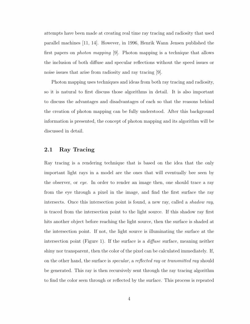
2.1 Ray Tracing

Ray tracing is a rendering technique that is based on the idea that the only

important light rays in a model are the ones that will eventually bee seen by

the observer, or eye. In order to render an image then, one should trace a ray

from the eye through a pixel in the image, and find the first surface the ray

intersects. Once this intersection point is found, a new ray, called a shadow ray,

is traced from the intersection point to the light source. If this shadow ray first

hits another object before reaching the light source, then the surface is shaded at

the intersection point. If not, the light source is illuminating the surface at the

intersection point (Figure 1). If the surface is a diffuse surface, meaning neither

shiny nor transparent, then the color of the pixel can be calculated immediately. If,

on the other hand, the surface is specular, a reflected ray or transmitted ray should

be generated. This ray is then recursively sent through the ray tracing algorithm

to find the color seen through or reflected by the surface. This process is repeated

4

for every pixel in the image (or several times per pixel), until a complete image is

created [5].

Figure 1: The ray tracing concept.

The color of each pixel is calculated by a combination of the amount of direct

light seen at the intersection point of the ray and the surface, the surface color

itself, and if the surface is specular, the color of the surface seen through a reflected

or transmitted ray. Some of the most important equations in ray tracing are listed

below [5, 13]. All vectors in the equations are unit vectors.

To calculate the color C of a diffuse surface with color S, normal �n, and at

position �s under a light with color L and position �l, the following is performed:

C = L · S(�n · (�l − �s)) (1)

To calculate the reflected direction �r of an incoming direction �d at a specular

surface with normal �n, the following is performed:

�r = 2(�n · �d)�n− �d (2)

5

To calculate the direction of a transmitted ray �t of an incoming ray with

direction �d at a specular surface with normal �n the following is performed: (Note:

the ray is traveling from a medium with refractive index m1 to a medium with

refractive index m2):

�t =m1(�d− �n)(�d · �n)

m2

− �n

√√√√1− m21(1− (�d · �n)2θ

m22

(3)

There is some disagreement between the terms “ray tracing” and “backward

ray tracing”. Some think “ray tracing” should be the process of tracing a ray from

the light to the eye, whereas other think it should the process of tracing a ray from

the eye to the light. For the rest of this paper, Glassner’s perspective will be used

and “ray tracing” will be defined as the rendering method suggests, tracing a ray

from the eye to the light, and “backwards ray tracing” will be defined as tracing

a ray from the light to the eye [5].

2.2 Radiosity

Radiosity is a rendering technique that takes into account the diffuse reflections

between surfaces. Because diffuse surfaces reflect energy in the form of heat and

light in all directions, it is possible for a surface that does directly “see” a light

or specular surface to receive illumination. This is exactly how real light behaves.

The inclusion of diffuse reflections adds reality to radiosity renderings(Figure 2)

which are nearly impossible with ray tracing [3].

Radiosity is a three-pass algorithm in which the first pass is dedicated to

calculating what are called form factors between two patches. Because an entire

wall can be a single polygon, it may be required to be broken into several smaller

polygons, or patches, so that shadows and illumination can be calculated correctly

6

Figure 2: A simple scene rendered with radiosity.

and as realistically as possible. A surface can be divided into patches uniformly or

by using algorithms such as adaptive subdivision to most efficiently subdivide each

surface in a given scene [3]. A single form factor between two patches represents

the percentage of the outgoing light from the first patch that is visible from the

second patch (Figure 3). In any given scene with n patches there are n2 − n form

factors (because a patch does not have a form factor with itself). Form factors can

be calculated through many different methods including the hemicube, source-to-

vertex, and hybridized algorithms [15].

The second pass takes all of the scene’s form factors along with the light

to be emitted from each light source and finds an equilibrium. An equilibrium

is found when all light transfer between patches no longer changes the current

illumination of any patch [3]. This may be done as one extremely large linear

equation, but to save time, a process called progressive refinement is suggested.

Progressive refinement iteratively uses the form factors to transfer energy from

the lights in the scene to the patches in the scene. In other words, progressive

refinement propagates the light throughout the scene one step at a time until the

7

Figure 3: The concept of form factors.

equilibrium is reached. Thus, light must first be transferred from the light sources

to all directly illuminated patches in the scene, then from all these patches to

every indirectly illuminated patch, and so on. There may be a need for numerous

iterations to reach an equilibrium in scenes where some patches only receive light

through several indirect reflections [15].

Finally, after an equilibrium is reached, the scene can be rendered using Gouraud

shading techniques in the third pass. API’s such as OpenGL can be used by in-

putting the scene geometry and applying a color to each vertex that corresponds

to the color calculated from the radiosity calculations. Thus, each patch in the

radiosity calculations will become a separate polygon in the rendered scene [3].

Typically, adaptive subdivision as mentioned above can be used to allow for

more accuracy and realism. In adaptive subdivision, each surface is divided into

patches based on knowledge of which areas of the surface will be shaded similarly.

This is usually done by computing a scene on a uniform subdivision, and is then

refined by adding patches where the uniform patches vary in color past a predefined

8

tolerance. By adding this step to the radiosity calculations, a more photorealistic

image can be produced than with only using a uniform subdivision [3].

2.3 Shortcomings of Ray Tracing and Radiosity

Both ray tracing and radiosity can produce exceptional images as can be seen in

Figures 2 and 4. However, there are many problems that keep them from creating

ultimately realistic images in a reasonable amount of time. Ray tracing does not

directly calculate diffuse reflections, color bleeding, or caustics, and it incorrectly

calculates light passing through specular surfaces. On the other hand, radiosity

cannot render specular surfaces without extreme complexity, and is extremely slow

[4].

Ray tracing’s first problem is that it does not include diffuse reflections. When

a ray traced through a pixel hits a surface, only the surface color, position of any

lights, and color of a reflected or transmitted ray (for specular surfaces only) are

included in the final color calculations. The effects of other surfaces in the vicinity

are not considered. This is of course not like real life and thus will not accurately

depict reality. Take for example a room as shown in Figure 4 where there is a light

source at the top of the room that only directly lights the floor and walls. In ray

tracing the ceiling will receive no illumination, which is quite contrary to reality.

Of course there have been additions to ray tracing that can help make images

more realistic such as Monte Carlo integration, path tracing, and soft shadows,

but these additions usually create noise and reduce speed greatly [9].

There are also several other phenomenon in real life that cannot be calculated

using simple ray tracing, one of which is color bleeding. If you were to place

a blue book perpendicular to a white wall you would see a slight hint of blue

transferred to the wall, even if the book isn’t glossy. Color bleeding requires diffuse

9

Figure 4: The unilluminated ceiling of a ray traced image.

reflections that will take into effect illumination from surfaces other than light

sources. Additionally, ray tracing cannot directly implement caustics. Caustics are

concentrated areas of light that are formed when specular surfaces focus reflected

or refracted light rays in close proximity. Examples of caustics are the focused

areas of light under a magnifying glass and the bright areas of light at the bottom of

a pool. Although there are techniques that use backward ray tracing to implement

caustics, because ray tracing itself was not designed to handle caustics, these

techniques are quite complicated and time consuming [6].

Ray tracing also has problems with calculating the behavior of light reflecting

off of or traveling through specular surfaces. Ray tracing does not account for light

that bounces off of a reflective material and illuminates previously shaded or less

illuminated areas. As shown in Figure 5, a sphere surrounded by mirrors should

have three shadows around it from the illumination off the mirrors and the light

source itself. However, ray tracing does not account for the illumination of the

sphere on any side except for the one directly visible from the light source. The

same type of problem occurs for transparent materials. Suppose a ray intersects a

10

wall that is partially shaded by a transparent sphere. The ray tracing algorithm

will create a shadow ray straight through the sphere, and because the sphere is

transparent the wall will receive illumination. However, the light being emitted

in the predicted direction will not illuminate that portion of the wall at all. The

transparent surface will redirect illumination to areas that a ray tracer cannot

predict (Figure 6).

Figure 5: The incorrectly illuminated sphere surrounded by mirrors.

Radiosity, as opposed to ray tracing, was designed to allow for the diffuse to

diffuse interaction between surfaces, but the cost of which is extremely expensive.

Because radiosity uses the form factors as percentages of transferred illumination,

radiosity can mimic both indirect illumination and color bleeding. Many of the

simple images that were generated using ray tracing looked much better when

generated through radiosity. Surface interaction becomes very lifelike as is visible

in the soft shadows of Figure 2, and the images look amazingly like photographs.

Another advantage of radiosity is its view-independent nature. Because the form

factors do not take into account a camera position, the illumination of each patch

can be reused if nothing moves within the scene. This is exceptionally useful in

11

Figure 6: The incorrectly illuminated wall though a transparent sphere.

creating quickly rendered walk-throughs [3].

However, these advantages are not without pitfalls. First of all, radiosity can-

not render specular surfaces. This inability is very severe in that not only can

radiosity not render transparent or reflective surfaces like glass and mirrors, but

it cannot render caustics at all. This shortcoming is one of the largest reasons for

the creation of photon mapping as will soon be explained. Another problem is the

complexity of rendering non-planar objects. Finding the form factors for spheres

and tori can be exceptionally complicated using algorithms like the hemicube tech-

nique [15]. This problem can be overcome by making meshes of these objects, but

this will only increase the amount of time required for rendering. Finally, radiosity

is inherently slow. Creating all of the form factors may not seem like a difficult

task but when we have a very complex scene with perhaps 1, 000 surfaces, 500 of

which come from converting a sphere into a triangle mesh, 1, 0002 or 1, 000, 000

form factors need to be computed. Even using progressive refinement cannot keep

the time required to render from being unacceptable in many situations.

12

There have been several attempts to combine radiosity and ray tracing tech-

niques creating a global illumination model with indirect illumination that can

still contain specular surfaces. Such examples of this are Radiance [12] and POV-

Ray [16]. Unfortunately all of the speed problems still remain, and are often

increased in these hybrid combinations. Obviously, a new technique that was as

versatile and quick as ray tracing while still including the indirect illumination

capabilities of radiosity was needed.

3 Photon Mapping

The need for an efficient yet completely illuminated rendering algorithm was an-

swered when Henrik Wann Jensen first created the two-pass “photon mapping”

algorithm in 1994 as part of his Ph.D. dissertation [9]. This algorithm achieved

everything that radiosity provided but with the speed, simplicity, and surface gen-

erality of ray tracing. The premise behind his method is simple; in the first pass

one simply shoots photons (photon tracing) from light the sources into the scene

and keeps track of the energy they give to encountered surfaces. Of course there

is no eye yet, but this is a two-pass algorithm; the camera will not appear until

the second pass. Whenever a photon hits a diffuse surface, it is stored in a data

structure called the global photon map. This is how diffuse reflections can be ac-

counted for. The second pass then uses ordinary ray tracing in conjunction with

the photons stored in the global photon map to capture all of the illumination

types currently needed in realistic image synthesis. The result of this combination

of both specular and diffuse reflections is a full global illumination model that can

capture many of the surface interactions that occur in real life.

It is strange to think that in the early years of ray tracing, tracing rays from the

light sources to the eye was once believed to be too complex and time consuming

13

[5]. Now, with the advances in computer speed and technology, this intuitive

approach can be reconsidered. A closer look at the two passes of the photon

mapping algorithm will now be given.

3.1 The First Pass: Creating the Global Photon Map

As previously stated, the first pass of the algorithm is to shoot photons from the

light sources and then store their progress in a data structure. In order to shoot

the photons we must know what type of light source we are dealing with. There

are several types of light sources as shown below [9].

• Point Light : A single coordinate in 3-dimensional space where photons can

be shot by randomly selecting any point on the unit sphere and shooting

them in that direction. Jensen suggests using rejection sampling to con-

strain random vectors inside the unit cube to those inside the unit sphere to

randomly generate point light photon emission.

• Square Light : This is, in general, the most popular type of light used in most

rendering techniques. It looks realistic, and is easy to implement. A square

light is simply a square surface that can emit photons from any point and

in any direction toward the normal. There are also several techniques using

square lights to allow for soft shadow generation.

• Complex Light : These are lights with an arbitrary shape that emit photons

at different proportions in different locations. The procedure of handling

these light sources will not be covered in this thesis.

Of course, if there are multiple lights in a scene, a light must be chosen before

a photon can be shot. However, one cannot simply choose a random light. The

14

probability of a light being selected must be proportional to the fraction of the

light’s power over the total amount of power from all lights in the scene [9].

Once the origin of the photon and its outgoing direction vector are known,

the photon can finally be shot. Using much the same algorithm as traditional

ray tracing, photon tracing finds the first surface that the photon would hit and

proceeds to update the global photon map in one of the following ways depending

on the type of surface intersected:

• If the photon hits a diffuse surface, store the photon’s energy and incident

direction into the global photon map.

• If the photon hits a specular surface, do nothing to the global photon map.

The global photon map will only consider photons that hit diffuse surfaces.

• If the surface is partially diffuse and specular, use what is called Russian

roulette to decide if at this particular instance the surface should be consid-

ered diffuse or specular. Russian roulette is simply the process of randomly

but proportionally choosing the outcome of a probabilistic situation.

In any case, whether the photon is absorbed or reflected by the surface must now

be decided. For either case Russian roulette is once again used with the surfaces

reflectivity property to see if the photon should be absorbed or reflected. If the

photon is absorbed, this particular photon’s life is ended here. If the photon is

reflected (or transmitted) the reflected ray must be calculated the process repeated

as if the photon started from the intersection point. Diffuse and specular surfaces

do not reflect photons in the same way, and these differences must be accounted

for. While specular surfaces can be assumed to reflect perfectly using Equation (2),

diffuse surfaces can reflect in any direction. This direction however is proportional

to the cosine of the angle between the perfectly reflected direction and the actual

15

reflected direction. To create the random reflection direction two random variables,

ξ1, ξ2 ∈ [0, 1] are needed. The reflected direction �r is then given by [9]:

�r = (θ, φ) = (cos−1(√ξ1), 2πξ2) (4)

Once a predefined number of photons have been scattered throughout the

scene, the photons must be sorted in a manner in which they can be easily retrieved

later. For reasons that will become obvious in the next section, Jensen suggests

using a k-d tree data structure to store the photons [9].

3.2 The Second Pass: Generating the Image

The second pass of the algorithm creates an image in much the same fashion as

ray tracing. It traces rays from the camera point through each of the pixels and

finds the first surface the ray encounters. The color given to the pixel depends

on the type of surface at the intersection point. If the surface is specular, a new

reflected or transmitted ray is generated and traced using Equations (2) or (3).

On the other hand, if the surface is diffuse, several sample reflected rays using

Equation (4) are created. For every reflected ray that hits another diffuse surface,

a radiance estimate at the intersection point is taken.

The radiance estimate finds the m closest photons in the photon map to the

inputted intersection point within some predefined distance (Figure 7). This is the

reason a k-d tree is suggested for the photon map. A k-d tree can easily traverse

a list of coordinates in three dimensions until the closest photon is found. This

can be done in O(log2 n) time for n total photons on average. Finding the next

m− 1 nearest neighbors is from this point a trivial task [10]. Along with the k-d

tree’s lack of memory overhead, it is obvious why it is a great candidate for the

photon map’s data structure. The radiance estimate is then found by totaling

16

the illumination of the m nearest photons and dividing by the area in which they

were found. This area is the area of the circle with a radius of distance from the

intersection point to the furthest of the m nearest neighbors [9].

Figure 7: How the radiance estimates are visualized.

Once all of the sample radiance estimates are found, they are averaged together.

This estimates the indirect illumination that the intersection point receives. This

can then be combined with the direct illumination from the light sources and any

specular properties to create an image using a global illumination model (Figure 8).

3.3 Color Bleeding and Photon Mapping

Because the radiance estimates of the photon mapping algorithm account for dif-

fuse reflections, it is possible to render color bleeding. Color bleeding can be

achieved simply by changing the color of the photons as they are reflected through-

out the scene. For example, if a white photon is reflected off of a blue wall, the

photon would now be blue, and the next time it hits a diffuse surface it should be

stored in the photon map as being blue. Unfortunately, Jensen fears that in order

17

Figure 8: Two photon mapped images.

to render color bleeding without what he calls “blotchy” effects would take more

than millions of photons [9]. However, this is not the case as can be seen from

Christensen’s work. Several of his images using 400, 000 photons can be seen to

exhibit quite realistic color bleeding [2].

3.4 Caustics and Photon Mapping

One major advantage of photon mapping is the ability to create wonderful caustics.

Jensen suggests keeping a second photon map called the caustics map to capture all

photons that have been reflected by or transmitted through a specular surface at

least once before hitting a diffuse surface. Once a photon hits a diffuse surface its

life should be ended. The caustics map however needs to be constructed carefully

to make sure that photons are not repeated in the global photon map. Once this

is added to the photon mapping algorithm, the final pixel value is a combination

of the direct, indirect, specular, and caustic illuminations [9].

18

4 Real Time Photon Mapping

In the graphics community it seems that as soon as an algorithm becomes estab-

lished, someone tries to make it faster. For years, the proponents of ray tracing

and radiosity discovered new ways to make each algorithm faster, more efficient,

and more realistic. The epitome of these improvements would be to have the algo-

rithms execute in real time. Radiosity had an advantage over ray tracing in that

it could easily render interactive walk-throughs. However, these walk-throughs

were not interactive. To accomplish real time interaction, one must account for

objects and light sources that move. Radiosity’s walk-throughs do not inherently

allow this; however, it seems easier to apply real time to radiosity because the

radiosity calculations are independent of the rendering technique. We can find

the form factors and the correct illuminations without having to worry about how

to render the scene. This allows radiosity to easily be rendered using OpenGL

or even ray tracing as hybrid techniques have shown. Ray tracing does not have

this advantage; it is the rendering technique itself and thus cannot be changed

without extensive effort. However, both ray tracing’s strong connection to the

rendering process and radiosity’s slow speed did not keep them from being used

to create real time algorithms. There are several examples of real time ray tracing

and real time radiosity systems available, many of which require parallel machines

to execute [11, 14].

Photon mapping has the benefit of once again having both ray tracing’s and

radiosity’s advantages while possessing none of their flaws. As with radiosity,

photon mapping is independent of the rendering process. Though most examples

of photon mapping use standard ray tracing to render, it is feasible to use other

methods. And while radiosity calculations become the bulk of the time complexity,

photon mapping itself takes a relatively small percentage of the rendering time.

19

It seems obvious that photon mapping can be transferred to the area of real time

interactive rendering. Furthermore, the speed of photon mapping is so fast that

it is also possible to perform real time rendering on a single processor machine.

4.1 The Concept

The concept of real time photon mapping is simple. Instead of shooting hundreds

of thousands or millions of photons once to render a scene, merely shoot tens or

hundreds of photons per frame. By limiting the number of photons shot, one

can minimize the per frame shooting time, making real time photon mapping not

only possible but practical. However, since tens or hundreds of photons will not be

adaquate to simulate the indirect illumination of a scene, the last several frames of

photons can be stored and reused. Once photons become old enough, they can be

overwritten by a newly shot frame of photons, thus keeping only the newest several

frames of photons maintained. Then, by using normal polygon-based rendering

methods such as OpenGL and a radiance estimate at each vertex of each polygon,

diffuse reflections and even color bleeding can be simulated. The process of real

time photon mapping can be broken down into three main stages which can be

seen through the algorithm outlined in Figure 9. These three stages: shooting the

photons, balancing the k-d tree, and applying the radiance estimate are dicussed

in detail in the following sections.

4.1.1 Stage 1: Shooting the Photons

There are three major issues in the first stage, the first two of which are choosing

a total number of photons and deciding how many photons to shoot per frame.

The third concerns choosing the distribution from which to shoot these photons.

Choosing how many total photons to shoot and how many photons to shoot

20

index := 1 // the index of the first photon to shoot per frameper frame := 100 // the number of photons to shoot per frametotal := 2000 // the total number of photons to storewhile true do

begin// Stage 1: Shooting the photons: Section 4.1.1shootPhotons(index, per frame)

// Stage 2: Balancing the k-d tree: Section 4.1.2balance()

// Stage 3: Rendering the image: Section 4.1.3for all polygons do

begin// find radiance estimate at each vertex// render polygon with illumination at vertices

end

index := (index+ per frame) modulo totalend

Figure 9: The proposed real time photon mapping algorithm

21

per frame is not a trivial task. Let total and per_frame represent these numbers

respectively. Both total and per_frame should be chosen carefully for several

reasons. Increasing per_frame will increase the number of photons that are shot

every frame, so shooting too many per_frame photons will obviously result in

slow processing times. Increasing total too much will also slow processing times

because more photon hits must be balanced and searched through for the radiance

estimates. Selecting too few per_frame or total photons will obviously decrease

the frame quality as the original photon mapping algorithm has shown [9]. How-

ever, by choosing a good balance between total and per_frame, one can create a

scene with reasonable results for any machine speed. Sections 5.1 and 5.3 discuss

further how changing these numbers will effect the output.

Once the number of photons to use are known, one can simply shoot per_frame

photons into the scene before each frame. However, it would be beneficial to

save and reuse the last frame’s photons because they are still relevant to current

conditions. Very small changes occur between frames when the frames are being

generated fast enough, so photons shot even a second ago can still give a proper

representation of the current scene. It is because of this that the total photons

are chosen. This number represents the maximum number of photons at any time

in the scene. Once the scene is filled with total photons, the oldest per_frame

photons are now irrelevant and can be thrown away and replaced with a newly

shot set of per_frame photons. Each frame then has at any given time a total

of total most recent photons. This process will be covered in more detail in

Section 4.1.2.

There is one more option that must be decided and that is the distribution

used to shoot the photons. A distribution in this sense is pattern in which the

photons are dispersed throughout the scene. There are three major options:

22

• Shoot every photon randomly into the scene.

• Shoot each per_frame set of photons with the same distribution.

• Shoot each total set of photons with the same distribution.

By shooting every photon randomly into the scene one can be assured that

over time, each possible path for a photon to take will be accounted for. Random

shooting is also very easy to implement. However, this will also result in some fluc-

tuation between frames because each frame overwrites its last per_frame photons

with ones shot in a completely different manner. This fluctuation can be lowered

by choosing an appropriate number of total photons and per_frame photons,

but changing these numbers can only effect the fluctuation slightly.

Shooting each frame of photons with the same distribution is the exact opposite

as random shooting. Every per_frame photons are shot with the same pattern

as the last per_frame photons. This method will keep any fluctuation between

frames to a minimum; however, this method may also keep areas of a scene from

being illuminated. Because the number of different paths the photons can travel is

limited to per_frame directions, the coverage of the photons is low. This results

in some sections of the scene being highly illuminated, and some being poorly

illuminated.

The last case is the suggested option: a distribution is chosen for the total

number of photons. This means that after total / per_frame frames have passed,

the distribution will be repeated. This allows for a good medium between low

fluctuation and high coverage.

4.1.2 Stage 2: Balancing the K-D Tree

Balancing the k-d tree, as covered in Section 3.2, is necessary for the radiance

estimate calculations. By using a k-d tree to store the photons, a minimum amount

23

of memory is used, while allowing the search of the nearest m photons to an

inputted hit point to be performed in O(log2(total)) time. A k-d tree is balanced

by choosing a median photon positioned along one of the coordinate axes and then

dividing the rest of the photons into two halves, the ones below the median and

the ones above it. This process is repeated by choosing the next axis and then

recursively balancing each of the halves. Figure 10 shows how a k-d tree divides

a set of two dimensional data.

Figure 10: How a k-d tree divides a set of two dimensional data.

Balancing of the k-d tree in the photorealistic photon mapping algorithm was

dependent on the maximum number of photons shot. In the proposed real time

photon mapping algorithm it will be dependent on the value of total photons. It

is suggested here that all of the photons be shot for the first frame. In this way the

illumination of the first frames will not be lacking. Now, for every frame there will

be on the order of total photons in the k-d tree that will need to be balanced.

Each frame the corresponding per_frame photons are simply overwritten with

new data.

The first problem that arises is how to handle diffusely reflected or specularly

24

reflected or transmitted photons. Because a photon may be reflected a different

number of times each time it is shot (this is due to either being randomly absorbed

or being reflected by a different object), a way to handle any number of reflections

must be created. This can be done in the following way. If a maximum reflection

level max_level is chosen (three has been seen to be sufficient for real time ren-

dering) then an array of max_level · total photon hit locations is needed. This

array of photon hits, called photons[ ], is conceptually broken into max_level

contiguous sections, with each section representing the first, second, etc. hits of

each of the total photons. The first time a photon with index i hits a surface its

information is put into position i in the array. The second time it hits a surface

its information is put into position (i + total) and so on (Figure 11). If a photon

hits a specular surface, the corresponding position in the array should be marked

as unused. The same should be done for all remaining positions if the photon is

absorbed through Russian roulette as described in Section 3.1.

Figure 11: The photons[ ] array with length total · max level.

Another problem is how to keep track of the photons in the k-d tree. Once

the k-d tree is balanced for each frame, the photons are no longer in the same

25

order they were in. This will make removing the oldest per_frame photons

and reshooting them extremely difficult. To overcome this, an array of inte-

ger indices, called photon_location[ ], can be created to show the position

in the photon array that a photon is currently located. Thus, when the bal-

ancing is performed, the photon_location[ ] array is updated along with the

photons[ ] array. Then removing and reshooting the oldest per_frame pho-

tons (starting with photon i) consists of simply updating the photons stored at

photons[photon_location[i, i+per_frame]] (Figure 12).

Figure 12: The photon location[ ] array and its relation to the photons[ ]

array.

4.1.3 Stage 3: Applying the Radiance Estimate

Now that the photons have been shot and the k-d tree has been balanced, we now

need to use that information to render the scene. By using the same radiance

estimate as used by the photorealistic photon mapping algorithm (Section 3.2),

we can find the diffuse illumination at each vertex in the scene. This will give us

a new type of realism in real time interactive programs that previously did not

26

exist.

The only real problem in this stage is choosing the number of photons to collect

in the radiance estimate. If we choose too many, then we will suffer slowdown in

this stage. If there are too few then we will have inaccurate estimation and dimmer

illumination [9].

4.2 Changes to the Photon Map

To accommodate for the real time photon mapping algorithm, we have to change

the photorealistic photon mapping algorithm slightly. While these changes may

modify the functionality, the concept behind the methods will not be altered.

The changes that must be made include additions to the Photon structure and

of the photon_location[ ] array, and changes to the functions that shoot all of

the photons, shoot a single photon, store a photon hit in the k-d tree, scale the

stored photon power, balance the k-d tree, and locate the photons for the radiance

estimates.

4.2.1 Additions to the Photon Mapping Algorithm

Because knowing which photons are not currently being used in the photon map is

essential, the first change to be made is in the photon itself. To allow for photons

to be skipped in the radiance estimate if they occurred at a specular surface or

were absorbed due to Russian roulette, we need to add a single bit flag called

used. If the photon is “live” and should be considered in the radiance estimate

we set the used flag to true. If not, we set the used flag to false. The new photon

structure should look like Figure 13.

Next, in order to remember which photon is which after the k-d tree is bal-

anced an integer array should be added to the photon map. This array is the

27

typedef struct Photonbegin

float pos[3];short plane;unsigned char theta, phi;float power[3];bool used;

end Photon;

Figure 13: The new Photon structure.

for i := 1 to total ·max level dobegin

photon location[i] := iend

Figure 14: Initializing the photon location[ ] array.

photon_location[ ] array and will contain the index in the photon array that

this photon is located at. This way, to know where photons[1] is located after

balancing, one looks at photons[photon_location[1]]. This array is initialized

in Figure 14.

4.2.2 Changing the Photon Shooting Functions

To allow for shooting only a select few photons into the scene every frame, a

change must be made to whatever function previously shot all of the photons (this

function will be referred to as shootPhotons()). Instead of shooting all of the

photons into the scene until the max number of storable photons is reached, one

must now be able to shoot a per_frame number of specific photons (or the total

number of photons if it is the first frame). This can be done by including both

28

shootPhotons(int num photons, int index)begin

level := 0photon ray := emitPhoton() // returns a ray from the lightlight power := getLightPower() // returns the light’s powerfor i := index to num photons do

beginshootOnePhoton(i, level, photon ray, light power) // Figure 16

endscalePhotonPower(index, num photons); // Figure 18

end

Figure 15: The function to shoot the per frame photons.

an int num_photons and an int index as parameters to the shootPhotons()

function. This way per_frame photons starting from a desired index can be shot.

When used in combination with the photon location array, photons can be shot

and reshot. The basic layout of the function to shoot the photons from a single

light source can be seen in Figure 15.

The shootOnePhoton() function as mentioned in Figure 15 must now be able

to shoot a single photon with the real time changes. Previously this function is

where the first surface the photon hit would be found. Russian roulette would then

be used to see if the photon was diffusely reflected, specularly reflected, specularly

transmitted, or absorbed. Only if the photon hit a diffuse surface would the photon

be stored, but now we must store the photon in every case so that previous data

can be overwritten. The new function for shooting a single photon can be seen in

Figure 16.

29

shootOnePhoton(int index, int level, Ray p ray, Vector power)begin

if level ≥ max level then returnp dir := p ray.direction // the Vector direction of the rayif (p ray intersects an object at hit point)

thenif (object is specular)

then// find reflected or transmitted ray r raystore(index+ (level · total), power, hit point, p dir, false)shootOnePhoton(index+ total, level + 1, r ray, power)

endifelse if (surface is diffuse and absorbed)

thenstore(index+ (level · total), power, hit point, p dir, true)for i := level + 1 to max level do

beginstore(index+ (i · total), power, hit point, p dir, false)

endendif

else if (surface is diffuse and reflected)then

// find diffusely reflected ray r dirstore(index+ (level · total), power, hit point, p dir, true)shootOnePhoton(index+ total, level + 1, r ray, power)

endifendif

end

Figure 16: The function to shoot a single photon.

30

store(const int index, Vector power[3],Vector pos[3], Vector dir[3], bool used)

beginPhoton node := photons[photon location[index]]node.used := usednode.pos := posnode.power := powernode.dir := dirUpdate bounding box for k-d tree if needed.

end

Figure 17: The function to store a photon hit in the photons[ ] array.

4.2.3 Changing the K-D Tree Functions

The store() function is used to record the position of a photon hit into the k-d

tree. As can be seen in Figure 16, changes to this function as suggested by Jensen

must be made [9]. This is because now a specific photon must be stored, and

it may also be the case that the photon should be flagged as “not used.” These

changes can be completed by adding a few more parameters: a bool used and an

int index. If used is true, then the photon’s used flag should also be set to true.

If false, the used flag should be set to false. This allows us to overwrite photons so

that if they were used in the previous frame, they will not be used in the current

frame or vice versa. The index is included to point to the correct photon. This is

the original index of the photon however, so the photon_location[ ] array must

be used. The bounding box used for the k-d tree does not need any changes as one

might suspect. Because the bounding box is only used to find a suitable median

for the k-d tree an appropriate amount of photons should always have the same

bounding box frame after frame. The revised photon storing function can be seen

in Figure 17.

31

scalePhotonPower(const float scale, const int num photons,const int index)

beginfor j := 0 to max level do

beginfor i := 0 to num photons do

beginloc := i+ index+ (j · total)Photon node := photons[photon location[loc]]node.power[0] := node.power[0] · scalenode.power[1] := node.power[1] · scalenode.power[2] := node.power[2] · scale

endend

end

Figure 18: The function to scale the newest per frame photons’ power.

When the photons in the photons[ ] array are stored, they are initially given

the same power as the light source they were emitted from. However, each photon

only has a fraction of this power, so each of the newly shot per_frame photons’

power must be scaled. In order to scale the photon power of the correct photons

we must also change the scalePhotonPower() function as proposed by Jensen [9].

Previously, in the photorealistic photon mapping algorithm, all of the photons were

scaled at once without regard to their current locations in the k-d tree. This is no

longer the case. Thus, the changes required are to use the photon_location[ ]

array to scale the correct per_frame photons. This keeps photons from being

scaled more than once, and keeps newly reshot photons from not getting scaled at

all. The changes to the scaling function can be seen in Figure 18.

During the k-d tree balancing in the balance() function, a photon’s index will

be changed in order to create the balanced tree. This requires a change to the

32

original code so that the position of each photon can be kept. This way shooting

photons 1 through 100 will still shoot photons 1 though 100 after the balancing.

This can be done by updating the photon_location[ ] array while the balancing

is being performed. The changes to the balancing function are quite simple so they

will not be shown. The needed changes must make sure to swap the values in the

photon_location[ ] array every time the photons in the photons[ ] array are

swapped.

4.2.4 Changing the Radiance Estimate Functions

Finally, we must make changes to the radiance estimate to ignore any photons

that have their used flags set to false. Thus, a photon with its used flag set to

false will not be a nearest photon to the point in question. This may add time

to the duration of the radiance estimate but it will be negligible. To make these

changes simply ignore any photons whose used value is set to false (These changes

are simple as well so they will not be shown).

4.3 Using Subdivision for More Detail

In many cases the original scene geometry may not provide enough detail in the

final rendering. In this case it may be advantageous to use an algorithm similar

to adaptive subdivision. By correctly choosing locations to divide a surface into

smaller more precise patches, we could increase the detail of our scene. Unfortu-

nately adaptive subdivision uses a “trial” version of the scene to discover which

areas need to be subdivided. Because of the lack of time for a real time system to

perform a “trial” version, a uniform subdivision may be all that can be done.

33

4.4 Speed Issues

There are several key places in the real time photon mapping algorithm that may

affect rendering speed. Because the algorithm is real time, all speed issues are

the most important issues even above realism and quality and as such should be

discussed. Those areas that have non-trivial solutions will be discussed in detail

later in this section with their possible solutions. The following are the areas in

question:

Shooting the Photons: The number of photons that will be shot per frame is

of major importance in how fast a frame can be rendered. This per_frame

number should be chosen as the number that can most accurately illuminate

the scene while still being fast enough to render enough frames per second.

Some guidelines for picking this value are given in Table 1.

Finding Hit Points: The time required to find the surface a photon hits is di-

rectly proportional to the number of surfaces in the scene. Since we cannot

simply require scenes to have few surfaces, we must use other techniques

to limit the surfaces checked for intersection. More on this topic will be

discussed in Section 4.4.1.

Balancing the K-D Tree: The total number of photons used is obviously the

major factor in how long balancing the k-d tree takes. As more photons are

included, the time for balancing will grow accordingly. Although O(n log2 n)

is quite fast for the balancing, it may be necessary and possible to speed it

up. A solution to this problem has not yet been found and the problem itself

is a major topic for future work.

The Radiance Estimate: The speed the radiance estimate takes is based on

how many photons are desired. A greater number will give better results (to

34

an extent) while a smaller number will be faster. However, because finding

more neighbors after the first neighbor is found is trivial, the time spent for

a single radiance estimate cannot be changed much.

Selecting Vertices to Render: Although the time spent finding a single ra-

diance estimate cannot be changed much, if there are many vertices in the

scene, the total time spent doing radiance estimates may become large. Thus

we must use techniques that can limit the number of radiance estimates per-

formed to only ones that effect what is displayed. More on this topic will be

discussed in Section 4.4.2.

4.4.1 Checking Fewer Surfaces for Intersection

The issue of finding the surface that a photon hits first is one that has been studied

extensively for ray tracing. Because photons go through the same process that

rays go through, the techniques discovered for ray tracing can be directly applied

for photon mapping in general. Some of these techniques are listed below.

Bounding Volume Hierarchies: By placing a bounding volume such as a sphere

or box around a set of objects, testing to see if a photon hits one of the ob-

jects within becomes much simpler. If this is done for many or all of the

objects in a scene, finding the intersection of a surface and the photon be-

comes a hierarchical process of searching first the bounding volumes and

then the objects inside. These objects may be the surfaces themselves or

other bounding volumes [6].

Space Subdivision: Breaking up the scene into a set of three-dimensional cells

can provide a way to speed up intersection times as well. Each cell will have

a list of all the objects that are inside it. When a photon reaches a cell, it will

35

check with all the objects in the cell’s list to see if there is an intersection,

if there is none, the photon is propagated to the next cell. The creation of

the cells can be uniform or adaptive, and a surface may lie in any number

of cells simultaneously [6].

Directional Subdivision: By subdividing the space into regions based on the

distribution of the photons, it is possible to receive better results than space

subdivision. This algorithm is nearly the same as space subdivision except

that the cells are created not as boxes of the environment but as pyramid

shaped volumes that represent similar directions a photon can be shot [6].

These algorithms all work well, but photon mapping has a property that can

be exploited to help reduce the number of surfaces checked further. An advantage

of the photon map is that it is separate and independent of the geometry of the

scene. Using this attribute we can perform a single scene simplification and still get

good results. Suppose the rendering of a set of books in real time (Figure 19). The

photon map itself doesn’t need to know all of the geometry of the books including

the curved bindings and covers. It simply needs to know the general perimeter

of the books in which photons should be stored on. Since the radiance estimates

will depend on proximity instead of exact location, the books can be replaced by

a single box and still be rendered with high quality (Figure 19). However, this

requires two versions of the scene: one to be rendered and one to use for photon

shooting. If desired, one can input each scene twice from two different source files.

This scene simplification can reduce the number of surfaces greatly in a scene and

make the photon shooting stage much quicker. See Section 5 for some results.

36

(a) (b)

Figure 19: An example of scene simplification from (a) an original model to (b) areduced model.

4.4.2 Fewer Radiance Estimates

For the same reasons that the number of surfaces checked for intersection should

be reduced, the number of vertices that perform a radiance estimate should also be

reduced. Because each vertex in the scene is the location of a radiance estimate,

the more vertices that can be discovered to be uneventful, the more time can be

saved. Of course, discovering if a vertex will affect the scene is more than simply

checking if the vertex will be seen. If any portion of the polygon can be seen, then

all of its vertices are eventful, and thus a radiance estimate should be performed.

There are several methods for performing this needed vertex removal, some of

which are outlined below:

Hidden-Surface Removal If at any time a polygon cannot be seen at all, all

of its vertices should be withheld from performing radiance estimates. This

includes any polygons that are not in the viewing frustrum or are totally

obscured by other polygons. A good algorithm used to perform this is the

z-buffer algorithm [1].

37

Back Face Culling Approximately one forth of the polygons in any given frame

are facing away from the camera. As long as there are no “thin” objects

in the scene, these polygons can also be ignored as well as their vertices. If

the angle between the camera ray and the surface normal is less than ninety

degrees, the surface can be ignored for this frame[1].

There is also another way of decreasing the number of radiance estimates

required to render a frame. By realizing that many polygons share vertices, we

can perform only one radiance estimate for the vertex and share the information

between the polygons. This can be done by connecting each of a polygon’s vertices

with a corner (Figure 20). Instead of finding the illumination at each vertex, the

illumination is found at each corner. Then, each vertex is rendered with the

illumination found at its corresponding corner. Some results of vertex cornering

and back face culling can be seen in Section 5.

Figure 20: Reducing the number of radiance estimates using corners.

38

5 Results

The proposed real time photon mapping algorithm is of little practicality if it

cannot render frames fast enough. On the other hand, if the visual results do not

show the phenomena expected, the algorithm will be superfluous. Because of this,

several tests need to be performed. These tests include changing the important

parameters of the algorithm to generate performance statistics, determine speedup

capabilities, and verify the visual quality of the results. Several phenomena that

can be performed using real time photon mapping will also be presented and

visually verified.

5.1 Performance

Performance statistics are probably the most important statistics for any real time

algorithm because they prove that the algorithm can be executed fast enough to

be performed in real time and fast enough not to be visually distracting. These

statistics also show how changing the values of different variables effect the speed in

which frames can be generated. All of the statistics in this section were performed

on a 866MHz Pentium III machine. Furthermore, each of the total per frame

rendering times are broken down into the algorithm’s three stages: shooting the

photons, balancing the k-d tree, and calculating the radiance estimates.

Figure 21 shows how changing the value for per_frame effects the per frame

rendering times. Each test scene consisted of 16 surfaces, 2, 000 total photons,

a max_level of 3, 100 photons in each radiance estimate, and a 512 by 512 pixel

output window. The first thing one should notice is that even as the number of

per_frame photons increases, the total rendering time is less than 0.06 seconds.

Although a scene should be rendered at a rate of roughly one frame every 0.05

seconds to seem fluid to the human eye, these numbers are extremely optimistic.

39

The second point to notice is that as the number of per_frame photons increases,

only the time dedicated to the shooting of the photons increases. The balancing,

radiance estimate, and rendering times all remain constant. Finally, the moment

in which the times for the shooting and balancing stages are equal should be

noticed. This moment will be discussed further in Section 5.3.

0 50 100 150 200 250 300 350 4000

0.01

0.02

0.03

0.04

0.05

0.06

per_frame Photons

Sec

onds

ShootingBalancingEstimatesTotal

Figure 21: The per frame rendering times as per frame is increased.

Figure 22 shows how changing the value for total effects the per frame ren-

dering times. Each test scene consisted of 16 surfaces, 100 per_frame photons, a

max_level of 3, 100 photons in each radiance estimate, and a 512 by 512 pixel

output window. First of all, the per frame rendering time never exceeds beyond

0.04 seconds, which is plenty fast enough for fluid animation. Secondly, one should

notice that increasing the total photons increases the time for both the balancing

and radiance estimate stages of the rendering while all of the other stages remain

constant. As the number of total photons is doubled, the balancing time is also

doubled; however, the radiance estimate times do not. The time required for the

radiance estimate times increase at a much lower rate than the balancing stage

times as the total photons are increased. This is simply because balancing takes

40

O(n log2(n)) time and radiance estiamtes take O(log2(n)) time. Once again, the

moment in which the times for the shooting and balancing stages are equal should

be noted for discussion in Section 5.3.

500 1000 1500 2000 2500 3000 3500 40000

0.005

0.01

0.015

0.02

0.025

0.03

0.035

0.04

total Photons

Sec

onds

ShootingBalancingEstimatesTotal

Figure 22: The per frame rendering times as total is increased.

Figure 23 shows how changing the value for max_level effects the per frame

rendering times. Each test scene consisted of 16 surfaces, 100 per_frame photons,

2000 total photons, 100 photons in each radiance estimate, and a 512 pixel by

512 pixel output window. What one notices first is that every stage in process

increases as max_level is increased. Thus, it is highly important that the value

of max_level is kept as small as possible. Section 5.3 will show that a max_level

of 3 is plenty for real time rendering.

What can be learned from Figures 21, 22, and 23 is that the proposed real time

photon mapping algorithm can actually be performed in real time. Unfortunately,

as Figure 24 shows, as the number of surfaces in the scene are increased, the per

frame rendering times soon become much too slow for interactive purposes. The

times quickly rise above a single second per frame, which makes real time photon

mapping impractical for scenes with many surfaces. What is most important

41

1 1.5 2 2.5 3 3.5 4 4.5 50

0.005

0.01

0.015

0.02

0.025

0.03

0.035

0.04

0.045

0.05

max_level

Sec

onds

ShootingBalancingEstimatesTotal

Figure 23: The per frame rendering times as max level is increased.

is that only the shooting and radiance estimate stages add to the slow results.

Section 5.2 will show how the inclusion of the speedups presented in Section 4.4

can be used to reduce per frame rendering times so that photon mapping can still

be performed in real time.

0 500 1000 1500 2000 2500 3000 3500 40000

0.5

1

1.5

2

2.5

3

3.5

4

4.5

Number of Surfaces

Sec

onds

ShootingBalancingEstimatesTotal

Figure 24: The per frame rendering times as the number of surfaces is increased.

42

5.2 Speedup Performance

The results obtained in Section 5.1 work well for a simple scene with 16 surfaces

but in order to render more complex scenes in real time, some of the suggested

speed improvements must be used. A comparison of the benefit of these speedups

is thus quite important to the real time photon mapping algorithm.

Figure 25 shows how using scene simplification can be used to keep per frame

rendering times low as surfaces are increased. In each case, the number of surfaces

in the simplified scene is kept constant at 16. When compared to Figure 24, it

is obvious to see that the shooting stage is no longer a speed issue. Thus, as the

number of surfaces increases, as long as the number of surfaces checked stays the

same, speed problems resulting from the shooting stage will not occur.

0 500 1000 1500 2000 2500 3000 3500 40000

0.1

0.2

0.3

0.4

0.5

0.6

Number of Surfaces

Sec

onds

ShootingBalancingEstimatesTotal

Figure 25: The per frame rendering times as the number of surfaces is increasedunder scene simplification.

However, Figure 25 also shows that the time required by the radiance esti-

mates is now a major problem. This problem can be solved by using either back

face culling or vertex cornering in order to reduce the times required for radiance

estimates. Figure 26 shows how culling can keep some of the radiance estimates

43

from being performed resulting in faster rendering times. Figure 27 shows how

vertex corning can keep radiance estimates at the same position from being re-

peated. Though culling does reduce rendering times, vertex corning is shown to

be a major improvement in the radiance estimate times.

0 500 1000 1500 2000 2500 3000 3500 40000

0.5

1

1.5

2

2.5

3

3.5

Number of Surfaces

Sec

onds

ShootingBalancingEstimatesTotal

Figure 26: The per frame rendering times as the number of surfaces is increasedunder back face culling.

Figures 24 shows that if the number of surfaces the photons are checked with

is not reduced somehow, the photon shooting and radiance estimate phases will

dominate the frame rendering costs. However, Figures 25, 26, and 27 also show

that with the included speedups, the per frame rendering time can remain very

similar to that of Figure 21. This is an extremely important statistic because as

scenes get larger, a heavily time consuming stage will most likely mean producing

frames at a rate that is unacceptable to the human eye.

5.3 Visual Results

For an algorithm that is so heavily visually dependent, tests must not be performed

on numbers alone. The algorithm must not only run fast enough, but must look

44

0 50 100 150 200 2500

0.02

0.04

0.06

0.08

0.1

0.12

0.14

0.16

0.18

0.2

Number of Surfaces

Sec

onds

ShootingBalancingEstimatesTotal

Figure 27: The per frame rendering times as the number of surfaces is increasedunder vertex cornering.

realistic enough as well. Several screenshots of the proposed real time photon

mapping algorithm have been included in this section so that visual results can

be discussed.

Figure 28 shows a few frames of output with 100 per_frame photons, 2000

total photons, a max_level of 3, and 256 surfaces. The scene was a simple

box containing two other smaller boxes. The light source (an invisible point light

source) makes a circular motion around the room demonstrating how a changing

position of a light source can be handled by real time photon mapping. The glow

of light can be seen to move from frame to frame, giving the correct output for

simulating dynamic illumination.

Figure 29 shows the same scene but only renders the photon map, thus only the

positions of the photon hits can be seen. These frames show how the photon hits

change as the scene changes. The highly concentrated areas of photons show where

in the scene the brightest illumination should be. When compared with Figure 28,

a direct correlation between illuminated surfaces and highly concentrated areas of

photons can be shown. A larger version of some of the frames of this scene has also

45

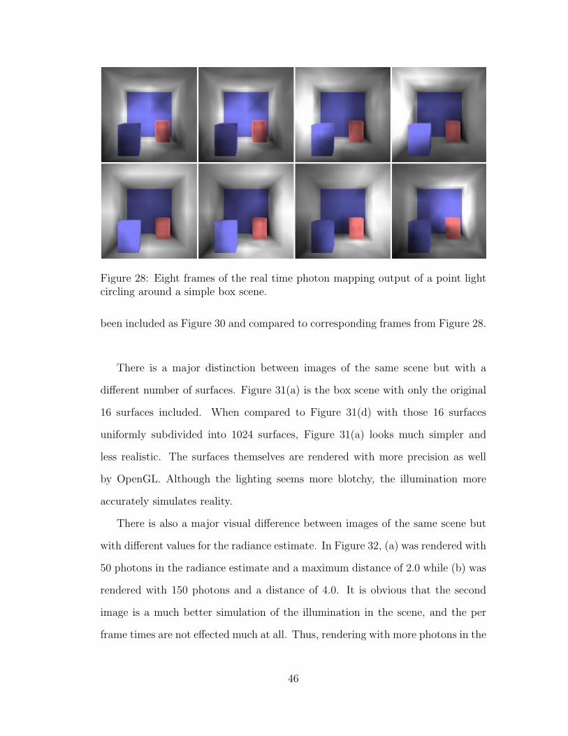
Figure 28: Eight frames of the real time photon mapping output of a point lightcircling around a simple box scene.

been included as Figure 30 and compared to corresponding frames from Figure 28.

There is a major distinction between images of the same scene but with a

different number of surfaces. Figure 31(a) is the box scene with only the original

16 surfaces included. When compared to Figure 31(d) with those 16 surfaces

uniformly subdivided into 1024 surfaces, Figure 31(a) looks much simpler and

less realistic. The surfaces themselves are rendered with more precision as well

by OpenGL. Although the lighting seems more blotchy, the illumination more

accurately simulates reality.

There is also a major visual difference between images of the same scene but

with different values for the radiance estimate. In Figure 32, (a) was rendered with

50 photons in the radiance estimate and a maximum distance of 2.0 while (b) was

rendered with 150 photons and a distance of 4.0. It is obvious that the second

image is a much better simulation of the illumination in the scene, and the per

frame times are not effected much at all. Thus, rendering with more photons in the

46

Figure 29: Eight frames of the photon hits of the simple box scene.

radiance estimate and a larger maximum distance gives more realistic, smoother

results with little cost to the rendering time. However, one must remember that

if the maximum distance is too large that photons will begin to be included in the

radiance estimate that are not appropriate for the vertex in question.

The visual effects of changing the number of per_frame photons and total

photons is slight when comparing only single frames. In order to see the difference,

one must view the animation itself. What can be seen when per_frame is too small

in comparison to total is that the illumination from the light source does not

appear until after the light has left its position. This can be stated more concisely

as the scene reacting too slowly to changes. This happens because there are too

many old photons still left in the scene that continue to show the illumination

in previous areas. On the other hand, if per_frame is too large in comparison

to total, then the illumination fluctuates. This is because there are too many

new photons being shot per frame and the random nature of the diffuse reflections

changes the illumination at each vertex greatly.

With the use of the per frame rendering times from Section 5.1 and these visual

47

Figure 30: Three frames of the box scene comparing the rendered image and thephoton hits.

48

(a) (b)

(c) (d)

Figure 31: The box scene rendered with (a) 16 surfaces, (b) 64 surfaces, (c) 256surfaces, (d) 1024 surfaces

49

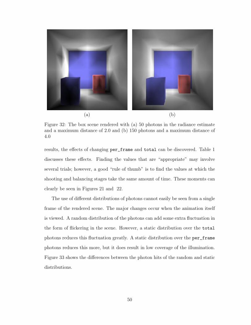
(a) (b)

Figure 32: The box scene rendered with (a) 50 photons in the radiance estimateand a maximum distance of 2.0 and (b) 150 photons and a maximum distance of4.0

results, the effects of changing per_frame and total can be discovered. Table 1

discusses these effects. Finding the values that are “appropriate” may involve

several trials; however, a good “rule of thumb” is to find the values at which the

shooting and balancing stages take the same amount of time. These moments can

clearly be seen in Figures 21 and 22.

The use of different distributions of photons cannot easily be seen from a single

frame of the rendered scene. The major changes occur when the animation itself

is viewed. A random distribution of the photons can add some extra fluctuation in

the form of flickering in the scene. However, a static distribution over the total

photons reduces this fluctuation greatly. A static distribution over the per_frame

photons reduces this more, but it does result in low coverage of the illumination.

Figure 33 shows the differences between the photon hits of the random and static

distributions.

50

Table 1: Photon number selection guidelinestotal per frame Result

Too small Too small Fast, inaccurate radiance estimates.Too large Illumination fluctuation.

Slow shooting time.Appropriate Fast results.

Slight illumination fluctuation.Too large Too small Scene reacts slowly to changes.

Slow balancing times.Too large Very slow processing times.Appropriate Scene reacts slowly to changes.

Slow balancing times.Appropriate Too small Inaccurate radiance estimates.

Too large Slight illumination fluctuation.Slow shooting times.

Appropriate Great results, good processing time.

5.4 Shadows and Color Bleeding

Besides allowing for diffuse reflections, real time photon mapping can be used to

add shadows to the scene. Each of the screenshots in Section 5.3 illustrates this.

This is achieved by storing every photon hit in the photon map so that direct

illumination is included as well. This will increase the number of photons needed

in the photon map, but the max_level of 3 can still be maintained. One direct

illumination level, and two indirect illumination levels are plenty for real time

rendering.

Another phenomenon that can now be performed in real time is color bleeding.

By using the same methods of simulating color bleeding in the original photon

mapping algorithm, it can be implemented in the real time version. Figure 34

shows the box scene rendered with color bleeding. A large difference can be seen

when the light is closest to the blue wall in the back of the room and when the

light is closest to the red wall behind the camera.

51

(a) (b)

Figure 33: The differences between (a) random and (b) static photon shootingdistributions.

(a) (b)

Figure 34: Color Bleeding of (a) a blue wall and (b) a red wall in real time photonmapping.

52

6 Conclusion

Interactive rendering has for a long time been limited to local illumination and

only recently has seen an inclusion of estimations of global illumination. Real time

ray tracing and radiosity techniques have been introduced, but can only lead to

frustrating shortcomings inherent in each algorithm. There are additions to both

ray tracing and radiosity that can be used to correct these shortcomings, but they

take extremely long amounts of time for a single image, let alone an interactive

setting. However, by using the concepts in photon mapping to create a real time

global illumination system, interactive graphics programming can be taken to a

new level of realism that includes diffuse reflections, shadows, and color bleeding.

And, as processing power increases, instead of simply catching up with the speed

required for real time ray tracing and radiosity, real time photon mapping can be

well on its way to practical and everyday use.

In this thesis we have modified the original photon mapping algorithm, an

algorithm for rendering extremely realistic images, and adapted it to run in an

interactive environment. We have demonstrated that, for the examples shown, it is

possible to render a photon mapped scene with 256 surfaces at a rate of 40 frames

per second. These results are due to the implicit speed of the photon mapping

algorithm and several improvements described in this thesis.

Many additional features can be added to improve the proposed algorithm;

however, there are a few topics that we believe are of the upmost importance to

the practicality and realism of real time photon mapping.

Balancing the K-D Tree: The time required to balance the k-d tree takes far

too long in comparison to how little work it is doing. The fact that only a

fraction of the photons are being rebalanced is incentive enough to find a

way to balance the k-d tree faster by using knowledge of other structures.

53

Perhaps an inserting, deleting, or merging function can be used to speed up

the balancing process. There may even be a way to remove the k-d tree

entirely, removing the balancing stage altogether.

Specular Surfaces: Another topic for future work is combining some of the work

on real time ray tracing with real time photon mapping so that specular

surfaces can be rendered as beautifully as ray tracing renders them but in

real time. Achieving this would certainly add another level of realism to

interactive rendering.

Caustics: It seems reasonable that caustics could be implemented by extending

this research. Proving that such phenomenon can be rendered in real time

would also add another level of realism.

Surface Subdivision: A method that may prove to be useful for subdividing

the surfaces in a scene would be to find areas of highly concentrated photons

during the balancing process, these areas could then be reduced to a single

vertex each and incorporated into the scene. This could be a method of

finding caustic locations as well.

Fluctuations: The visual results of the proposed real time photon mapping algo-

rithm show some undesired fluctuation that cannot be corrected by simply

adjusting the total and per_frame photons. A way of reducing this fluc-

tuation would be another worthwhile research topic.

54

A List of Variables

Variable Type Description 1st Reference

ξ1 double Random variable Section 3.2ξ2 double Random variable Section 3.2θ double Spherical angle Section 3.1φ double Spherical angle Section 3.1C RGB color The color given to a pixel. Section 2.1�d Vector The incident direction. Section 2.1dir Vector A direction vector. Figure 16hit_point Vector The position on a surface that

a photon has hit. Figure 17i int A loop variable. Section 9index int The currently chosen index of

an array. Figure 9L RGB color The color of a light. Section 2.1�l Vector The position of a light source. Section 2.1level int The number of reflections a

photon has gone through. Figure 15light_power Vector The color and intensity of an

emitted photon. Figure 15loc int The current location in the

photon_location[ ] array. Figure 18m1 double Index of refraction. Section 2.1m2 double Index of refraction. Section 2.1max_level int The maximum times a photon can

be reflected or transmitted. Section 4.1.2�n Vector The surface normal of a surface. Section 2.1node Photon A single photon to store. Figure 17num_photons int The current number of photons

to iterate through. Figure 15per_frame int The number of photons to shoot

each frame. Section 4.1.1

55

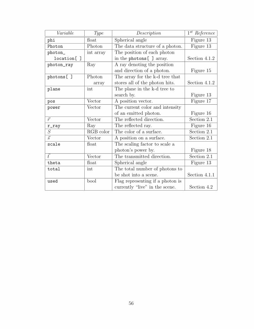
Variable Type Description 1st Reference

phi float Spherical angle Figure 13Photon Photon The data structure of a photon. Figure 13photon_ int array The position of each photon

location[ ] in the photons[ ] array. Section 4.1.2photon_ray Ray A ray denoting the position

and direction of a photon. Figure 15photons[ ] Photon The array for the k-d tree that

array stores all of the photon hits. Section 4.1.2plane int The plane in the k-d tree to

search by. Figure 13pos Vector A position vector. Figure 17power Vector The current color and intensity

of an emitted photon. Figure 16�r Vector The reflected direction. Section 2.1r_ray Ray The reflected ray. Figure 16S RGB color The color of a surface. Section 2.1�s Vector A position on a surface. Section 2.1scale float The scaling factor to scale a

photon’s power by. Figure 18�t Vector The transmitted direction. Section 2.1theta float Spherical angle Figure 13total int The total number of photons to

be shot into a scene. Section 4.1.1used bool Flag representing if a photon is

currently “live” in the scene. Section 4.2

56

References

[1] Angel, Edward, Interactive Computer Graphics, Addison-Wesley, Reading,Massachusetts, 1997.

[2] Christensen, Per H, Faster Photon Map Global Illumination, The Journal ofGraphics Tools, Vol. 4, No. 3, 1999.

[3] Cohen, Michael F. and John R. Wallace, Radiosity and Realistic Image Syn-thesis, Academic Press Professional, Boston, 1993.

[4] Foley, James D., Andries van Dam, Steven K Feiner, and John F. Hughes,Computer Graphics: Principles and Practice, Second Edition, Addison-Wesley, Reading, Massachusetts, 1990.

[5] Glassner, Andrew S. Editor, An Introduction to Ray Tracing, Academic Press,London, 1989.

[6] Glassner, Andrew S., Principles of Digital Image Synthesis, Two Volumes,Morgan Kaufmann, San Francisco, 1995.

[7] Gonnet, G.H., Handbook of Algorithms and Data Structures, Addison-Wesley,London, 1984.

[8] Jensen, Henrik Wann, Rendering Caustics on Non-Lambertian Surfaces,Graphics Interface ’96, May 1996, pp.116-121.

[9] Jensen, Henrik Wann, Realistic Image Synthesis Using Photon Mapping, AK Peters, Natick, Massachusetts, 2001.

[10] Marner, Jacob, KD Tree Demo, May 2000,http://www.rolemaker.dk/nonRoleMaker/uni/algogem/kdtree.htm.

[11] Muuss, Michael John, Towards Real-Time Ray-Tracing of CombinatorialSolid Geometric Models, Proceedings of BRL-CAD Symposium ’95, June1995, pp.5-9.

[12] Larson, Greg Ward and Rob Shakespeare, Rendering with Radiance, MorganKaufmann, San Francisco, 1998.

[13] Shirley, Peter. Realistic Ray Tracing, A K Peters, Natick, Massachusetts,2000.

[14] Stuttard, David, Adam Worrall, Derek Paddon, and Claire Willis, A Radios-ity System for Real Time Photo-Realism, Computer Graphics: Developmentsin Virtual Environments, June 1995, pp.71-81.

[15] Watt, Alan and Mark Watt, Advanced Animation and Rendering Techniques:Theory and Practice, Addison-Wesley, New York, 1992.

57

[16] Young, Chris and Drew Wells, Ray Tracing Creations, Second Edition, WaiteGroup Press, 1994.

58