Real-time Musical Score Following from a Live Audio Source · PDF fileReal-time Musical Score...
33
Real-time Musical Score Following from a Live Audio Source Andrew Lee Maneesh Agrawala, Ed. Carlo H. Séquin, Ed. Electrical Engineering and Computer Sciences University of California at Berkeley Technical Report No. UCB/EECS-2014-127 http://www.eecs.berkeley.edu/Pubs/TechRpts/2014/EECS-2014-127.html May 22, 2014
Transcript of Real-time Musical Score Following from a Live Audio Source · PDF fileReal-time Musical Score...
Real-time Musical Score Following from a Live Audio
Source
Andrew LeeManeesh Agrawala, Ed.Carlo H. Séquin, Ed.
Electrical Engineering and Computer SciencesUniversity of California at Berkeley
Technical Report No. UCB/EECS-2014-127
http://www.eecs.berkeley.edu/Pubs/TechRpts/2014/EECS-2014-127.html
May 22, 2014
Copyright © 2014, by the author(s).All rights reserved.
Permission to make digital or hard copies of all or part of this work forpersonal or classroom use is granted without fee provided that copies arenot made or distributed for profit or commercial advantage and that copiesbear this notice and the full citation on the first page. To copy otherwise, torepublish, to post on servers or to redistribute to lists, requires prior specificpermission.
Acknowledgement
I thank the Electrical Engineering and Computer Sciences department atUC Berkeley for funding my Masters year. I would like to thank my researchadvisor Maneesh Agrawala and my reader Carlo Séquin for all of their helpand guidance during my graduate education. The work described in thispaper was done in the context of the final project for the UC Berkeleycourse User Interface Design and Development, and I would like to thankManeesh Agrawala and Björn Hartmann for teaching it. Finally, I would liketo thank my family and friends for supporting me throughout the year.
Real-time Musical Score Following from a Live Audio Source
by Andrew Lee
Research Project
Submitted to the Department of Electrical Engineering and Computer Sciences,University of California at Berkeley, in partial satisfaction of the requirements forthe degree of Master of Science, Plan II.
Approval for the Report and Comprehensive Examination:
Committee:
Professor Maneesh AgrawalaResearch Advisor
(Date)
* * * * * * *
Professor Carlo H. SequinSecond Reader
(Date)
Acknowledgments
I thank the Electrical Engineering and Computer Sciences department at UC Berkeley for funding my
Masters year.
I would like to thank my research advisor Maneesh Agrawala and my reader Carlo Sequin for all of their
help and guidance during my graduate education.
The work described in this paper was done in the context of the final project for the UC Berkeley course
User Interface Design and Development, and I would like to thank Maneesh Agrawala and Bjorn Hartmann
for teaching it.
Finally, I would like to thank my family and friends for supporting me throughout the year.
2
Abstract
Musical score following has many practical applications. As mobile devices get more popular, musicians
would like to carry their sheet music on their mobile devices. One useful functionality that a sheet music
app could offer is to have the app follow the music being played by the musician and turn pages at the
right time. In this paper, we describe how we combined several techniques to accomplish this task and how
we implemented it to run efficiently. By understanding basic sheet music semantics and how instruments
produce sound, we carefully constructed a hidden Markov model to follow a player’s position in a musical
score solely by listening to their playing. We implemented our algorithm in Java, in the form of a sheet
music application for Android, and it was able to successfully follow amateur-level pianists playing Twinkle
Twinkle Little Star, as well as Minuet in G, by J.S. Bach.
3
Contents
1 Introduction 6
2 Related Work 7
3 Algorithm 8
3.1 Hidden Markov Model Formulation . . . . . . . . . . . . . . . . . . . . . . . . . . . . . . . . . 8
3.1.1 The Hidden State . . . . . . . . . . . . . . . . . . . . . . . . . . . . . . . . . . . . . . 8
3.1.2 The Observable State . . . . . . . . . . . . . . . . . . . . . . . . . . . . . . . . . . . . 10
3.1.3 Using the Forward Algorithm . . . . . . . . . . . . . . . . . . . . . . . . . . . . . . . . 10
3.2 Designing the Emission Distributions . . . . . . . . . . . . . . . . . . . . . . . . . . . . . . . . 11
3.2.1 Musical Note Mechanics . . . . . . . . . . . . . . . . . . . . . . . . . . . . . . . . . . . 11
3.2.2 Probability Computation . . . . . . . . . . . . . . . . . . . . . . . . . . . . . . . . . . 13
3.3 Designing the Transition Probabilities . . . . . . . . . . . . . . . . . . . . . . . . . . . . . . . 14
3.3.1 Restricting Transitions by Page . . . . . . . . . . . . . . . . . . . . . . . . . . . . . . . 16
4 Implementation 17
4.1 Goertzel Algorithm . . . . . . . . . . . . . . . . . . . . . . . . . . . . . . . . . . . . . . . . . . 17
4.2 Preprocessing . . . . . . . . . . . . . . . . . . . . . . . . . . . . . . . . . . . . . . . . . . . . . 18
4.3 Main Loop . . . . . . . . . . . . . . . . . . . . . . . . . . . . . . . . . . . . . . . . . . . . . . 18
4.4 Restricting the Considered States . . . . . . . . . . . . . . . . . . . . . . . . . . . . . . . . . . 19
4.5 Results . . . . . . . . . . . . . . . . . . . . . . . . . . . . . . . . . . . . . . . . . . . . . . . . . 19
5 Future Work 22
5.1 Understanding Tempo and Rhythm . . . . . . . . . . . . . . . . . . . . . . . . . . . . . . . . . 22
5.2 Extension to other Instruments . . . . . . . . . . . . . . . . . . . . . . . . . . . . . . . . . . . 22
5.3 Better Note Break Detection . . . . . . . . . . . . . . . . . . . . . . . . . . . . . . . . . . . . 23
5.4 Additional Considerations for a Useful App . . . . . . . . . . . . . . . . . . . . . . . . . . . . 23
5.4.1 Importing Sheet Music . . . . . . . . . . . . . . . . . . . . . . . . . . . . . . . . . . . . 23
5.4.2 Pagination and Page Transitions . . . . . . . . . . . . . . . . . . . . . . . . . . . . . . 23
6 Summary 25
A Observed Frequencies Table 27
4
B Computing N and k for each Observed Frequency 30
C Minuet in G Note Sets 31
5
Chapter 1
Introduction
Many piano players who use sheet music understand the annoyance of having to flip pages. In a live
performance, it is common to hire another person whose only task is to turn pages for the performer.
Otherwise, the piano player has turn the pages themselves, which requires taking their hand off the keyboard,
causing a disruption in their playing. Recently, some electronic products have emerged that allow hands-free
page turning for both physical and digital sheet music. However, they are usually foot-operated, so the
pianist still needs to execute a conscious action to flip the page.
We set out to create a mobile app that automatically advances pages for the player as they play, never
requiring them to perform any action outside of simply playing their piece. In other words, we want to
digitally replicate the job of the human page turner. This required a method to understand where in the
score the player is playing so we know when the player has reached the end of the page. Additionally, to make
it work on regular acoustic pianos without any special apparatus, we do not have the luxury of technologies
like MIDI to directly measure what keys the user is playing, so the only source of input we employ is sound.
It is this method which we will describe in this paper. Using a hidden Markov model with carefully designed
probabilities, we have developed an algorithm that can follow a player’s piano playing after being given the
musical score. Our algorithm has been fully realized in the form of a sheet music application for Android.
6
Chapter 2
Related Work
Our problem belongs to a field known as musical score following, which aims to find a correspondence between
a known musical score and a performance of that piece. In this field, the problems can be categorized into two
types: off-line and on-line. In the off-line case, which is sometimes called score matching, the performance
in its entirety has already been recorded, and thus, the approaches to this problem have the ability to “look
into the future” to better establish the correspondence. The on-line case does not have this luxury, as its
task is to continuously find this correspondence in real-time as the performer plays.
One class of approaches is based on dynamic time warping. As its name suggests, the goal is to warp
sequences in time to find a way to make them match. While its usefulness is evident in an off-line setting,
it is not as clear in an on-line setting, since the performance in the future is not available. Work has been
done to adapt dynamic time warping for streaming data [5, 6].
One of the most popular techniques to score following is to employ a hidden Markov model [4]. While
the specifics vary by approach, most define the hidden states in terms of the notes in the original score and
have the observable states correspond to the audio that is produced by those notes [8–10].
7
Chapter 3
Algorithm
Our goal is to infer where the player is currently playing within sheet music. While we cannot directly
measure where in the piece the player is consciously playing, we can indeed observe the sounds that they
produce using the piano. Formulating the problem in this manner naturally lends itself to an application of
the hidden Markov model.
3.1 Hidden Markov Model Formulation
To model our problem as a hidden Markov model, we need to define the hidden states and the observable
states.
3.1.1 The Hidden State
At a high level, we define the hidden state to be the player’s position in the piece. Specifically, we define
each state as a set of notes, which we aptly call a note set. When a given state is active, that means the
notes in that state are currently being emitted from the instrument.
The first step in determining our set of possible states is to generate a sequence of note sets {N0, N1, N2, . . .}by creating one at every onset of new notes in the score. Figure 3.1a depicts an example of how we do this.
Notice that for sections where a note is being held while new notes are being played, we only consider
the new notes for each note set. The reason we disregard the note after its original onset is because by the
time the new notes are played, the sound of the former may have died down and become overshadowed by
the latter.
If there are repeats or other control flow notations in the sheet music such as D.C. al Fine, we “unfold”
them beforehand, so that the sequence of note sets Ni is just a simple linear representation of the notes in
the score, in the order that the player will play them. Thus, as the player progresses through the music,
they would keep jumping to the following state as they play the notes.
We found that these Ni note sets alone were insufficient for our needs. This rudimentary formulation
assumes that the player is playing something at all times, and does not accommodate the case when the
player is at rest. To remedy this, we artificially create a note set Ri to follow each Ni. Every Ri is an empty
set, which represents the state of playing no notes. Semantically, if the player is currently at Ri, which we
8
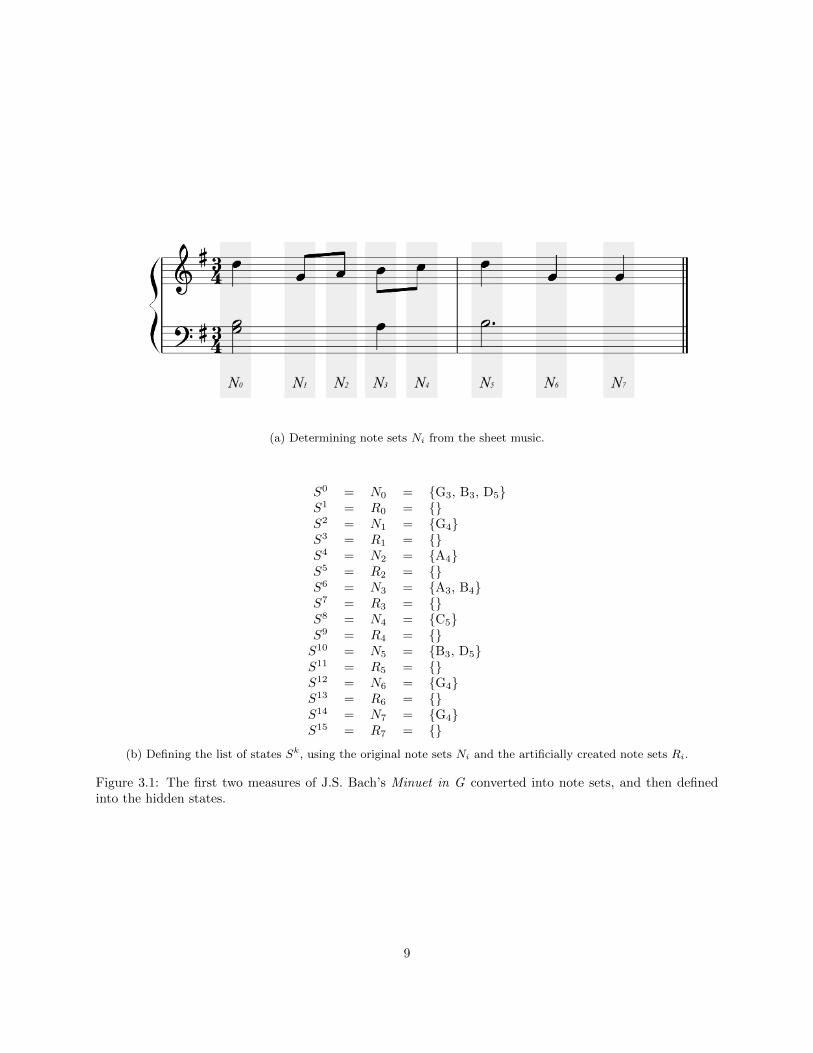
(a) Determining note sets Ni from the sheet music.
S0 = N0 = {G3, B3, D5}S1 = R0 = {}S2 = N1 = {G4}S3 = R1 = {}S4 = N2 = {A4}S5 = R2 = {}S6 = N3 = {A3, B4}S7 = R3 = {}S8 = N4 = {C5}S9 = R4 = {}S10 = N5 = {B3, D5}S11 = R5 = {}S12 = N6 = {G4}S13 = R6 = {}S14 = N7 = {G4}S15 = R7 = {}
(b) Defining the list of states Sk, using the original note sets Ni and the artificially created note sets Ri.
Figure 3.1: The first two measures of J.S. Bach’s Minuet in G converted into note sets, and then definedinto the hidden states.
9
call the rest state of Ni, that means they have stopped playing state Ni, or that they have held out the
notes in state Ni so long that the background noise overtakes the signal of the notes. Either way, it acts as
a holdover state while the player has not yet advanced to playing state Ni+1.
Now, we have finished defining the set of all possible states. For notation purposes, we will define Si as
the following:
Si =
N i2
if i is even
R i−12
if i is odd
In other words, {S0, S1, S2, S3, . . .} is the sequence of Ni interleaved with the sequence of Ri. Figure 3.1b
shows the result of this process, continuing the previous example.
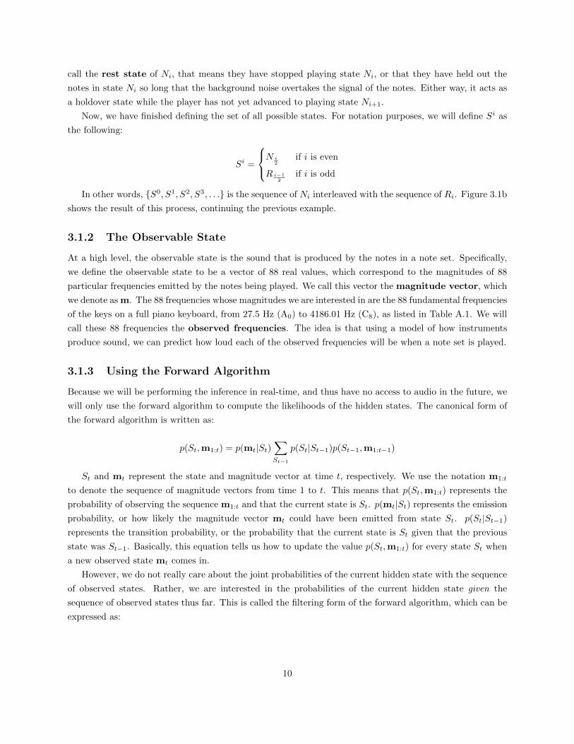
3.1.2 The Observable State
At a high level, the observable state is the sound that is produced by the notes in a note set. Specifically,
we define the observable state to be a vector of 88 real values, which correspond to the magnitudes of 88
particular frequencies emitted by the notes being played. We call this vector the magnitude vector, which
we denote as m. The 88 frequencies whose magnitudes we are interested in are the 88 fundamental frequencies
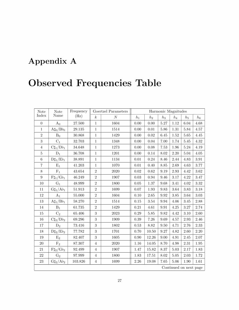
of the keys on a full piano keyboard, from 27.5 Hz (A0) to 4186.01 Hz (C8), as listed in Table A.1. We will
call these 88 frequencies the observed frequencies. The idea is that using a model of how instruments
produce sound, we can predict how loud each of the observed frequencies will be when a note set is played.
3.1.3 Using the Forward Algorithm
Because we will be performing the inference in real-time, and thus have no access to audio in the future, we
will only use the forward algorithm to compute the likelihoods of the hidden states. The canonical form of
the forward algorithm is written as:
p(St,m1:t) = p(mt|St)∑St−1
p(St|St−1)p(St−1,m1:t−1)
St and mt represent the state and magnitude vector at time t, respectively. We use the notation m1:t
to denote the sequence of magnitude vectors from time 1 to t. This means that p(St,m1:t) represents the
probability of observing the sequence m1:t and that the current state is St. p(mt|St) represents the emission
probability, or how likely the magnitude vector mt could have been emitted from state St. p(St|St−1)
represents the transition probability, or the probability that the current state is St given that the previous
state was St−1. Basically, this equation tells us how to update the value p(St,m1:t) for every state St when
a new observed state mt comes in.
However, we do not really care about the joint probabilities of the current hidden state with the sequence
of observed states. Rather, we are interested in the probabilities of the current hidden state given the
sequence of observed states thus far. This is called the filtering form of the forward algorithm, which can be
expressed as:
10
p(St|m1:t) ∝ p(mt|St)∑St−1
p(St|St−1)p(St−1|m1:t−1)
This form lets us renormalize the probabilities at the end after computing the sums for each possible
state. One of the great advantages of this normalization is that we can be more relaxed in the design of
our emission probability distribution, p(mt|St). Ultimately, the property that we want p(mt|St) to have is
that given mt, if we believe state Si is more likely than Sj to have emitted mt, then p(mt|Si) > p(mt|Sj).Rather than designing p(mt|St) such that it obeys the required probability properties, we can instead design
a function E that has the property, if state Si is more likely to have produced mt than state Sj , then
E(mt, Si) > E(mt, S
j). Thus, our update equation can be rewritten as:
p(St|m1:t) ∝ E(mt, St)∑St−1
p(St|St−1)p(St−1|m1:t−1)
3.2 Designing the Emission Distributions
To design a good emission distribution, we need to first understand what happens when notes are played on
the piano.
3.2.1 Musical Note Mechanics
A string with fixed ends has multiple frequencies that it can resonate at, called harmonics. We often call
the lowest harmonic the fundamental frequency (the one we perceive as the pitch of the note) and the other
ones overtones. If the string is ideal, the overtones exist at integer multiples of the fundamental. While a
real string’s overtones do not exactly correspond to integer multiples of its fundamental frequency (they are
typically slightly higher), in this application, they are close enough that we treat them as such.
Since the frequencies of the notes on a musical scale increase exponentially, while the harmonics are
spaced linearly in frequency, the overtones of a note actually space out in a logarithmic fashion. Musically
speaking, the first five overtones of a note occur roughly 12, 19, 24, 28, and 31 semitones above that note.
The important aspect is that when a string is struck, which is what happens inside a piano, multiple
harmonics of the string simultaneously ring out. Therefore, the sound that is produced contains not just the
fundamental frequency, but the overtones as well. It is the combination of these harmonics that characterize
the sound of an instrument, which we also call the timbre of the instrument.
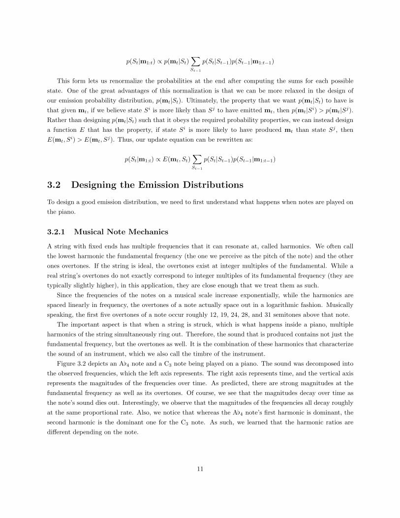
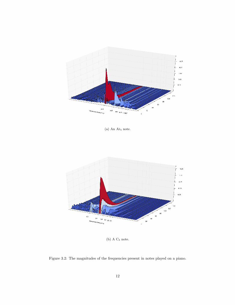
Figure 3.2 depicts an A[4 note and a C3 note being played on a piano. The sound was decomposed into
the observed frequencies, which the left axis represents. The right axis represents time, and the vertical axis
represents the magnitudes of the frequencies over time. As predicted, there are strong magnitudes at the
fundamental frequency as well as its overtones. Of course, we see that the magnitudes decay over time as
the note’s sound dies out. Interestingly, we observe that the magnitudes of the frequencies all decay roughly
at the same proportional rate. Also, we notice that whereas the A[4 note’s first harmonic is dominant, the
second harmonic is the dominant one for the C3 note. As such, we learned that the harmonic ratios are
different depending on the note.
11
(a) An A[4 note.
(b) A C3 note.
Figure 3.2: The magnitudes of the frequencies present in notes played on a piano.
12
Additionally, when multiple notes are played simultaneously, the resulting set of frequencies is observed
to be equivalent to superposing the frequencies produced by those notes individually.
Using these observations, we decided to characterize note sets by the ratio of the strengths of the harmonic
frequencies they exhibit. Using the A[4 note as an example, we can say that it is characterized with
having frequencies at A[4, A[5, E[6, A[6, C7, and E[7, where their magnitudes obey a ratio of roughly
10 : 6 : 3 : 3 : 2 : 1. Apart from background noise, this characterization is agnostic to the loudness of the
note(s) at any point in its duration. In the case of a note set where multiple notes are being played at the
same time, we assume that they are played at the same volume, so we construct the note set’s characteristic
harmonics by simply adding together the harmonic characteristics of the component notes. Even though it
is possible for the player to play the notes at different volumes, this does not happen often and we found
that our algorithm still performs well when they do.
3.2.2 Probability Computation
Because we characterize note sets by the ratios of the magnitudes of the harmonic frequencies, we encode this
description in the form of an 88-dimensional vector. A vector is a convenient form to encode this information
since no matter how it is uniformly scaled, its components will all remain in the same ratio.
First, we need to determine the first six harmonic magnitudes for each note played on a piano, with each
note played at the same volume. This was done empirically on a number of notes, and then interpolated for
the remaining ones. The values we settled on are listed in Table A.1.
Next, we will define the vector for any note n, which we denote n. Let n = 〈n0, n1, n2, . . . , n87〉. If h1,
h2, h3, h4, h5, and h6 are the first six harmonic magnitudes of n and the note index of n is i, then ni = h1,
ni+12 = h2, ni+19 = h3, ni+24 = h4, ni+28 = h5, and ni+31 = h6. The remaining components are 0. Thus,
n is more or less the magnitude vector we would expect from playing the note n.
Consequently, we define the vector of a note set S, which we denote S, as simply the vector sum of its
notes’ vectors. To account for background noise, we also add a vector b, which represents the magnitude
vector caused by background noise. Thus, we have:
S = b +∑n∈S
n
Finally, we normalize these note set vectors, denoting them as S:
S =S
‖S‖
When the incoming sound comes in, we extract the current magnitude vector mt from the signal using
the Goertzel algorithm, which is elaborated upon in Section 4.1. Then, our goal is to compare mt to the
unit vectors of each possible note set Si. Geometrically, the closer the ratio of the components in mt is
to that of Si, the more parallel the vectors are. Thus, to measure this notion, we use the dot product.
mt · Si = ‖mt‖‖Si‖ cos θ, where θ is the angle between the two vectors. Since Si is a unit vector, the
expression reduces to ‖mt‖ cos θ, meaning that only θ has any effect on the value. That means the dot
product is greater the more parallel mt is to Si, which is exactly what we wanted.
As mentioned in Section 3.1.3, we wish to define an emission function E that behaves like p(mt|St).
13
Intuitively, we want E(mt, St) to be greater if we believe that note set St is more likely to produce mt.
Thus, one way to define E is:
E(mt, St) = mt · St
However, we found that this function was not discriminating enough. To exaggerate the differences
between the regular dot product results, we square them:
E(mt, St) =(mt · St
)2We found that using higher exponents would make it too strict, so we settled on taking the square.
3.3 Designing the Transition Probabilities
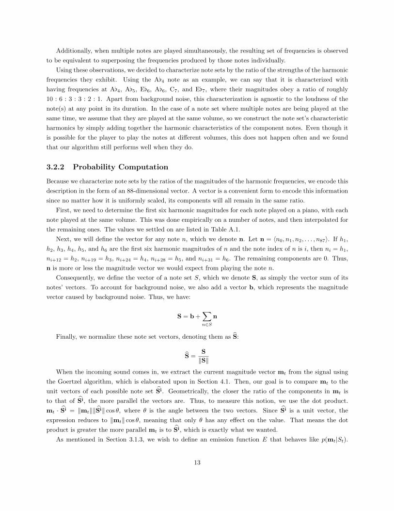
Figure 3.3: A partial sequence of note sets, along with arrows representing transition probabilities.
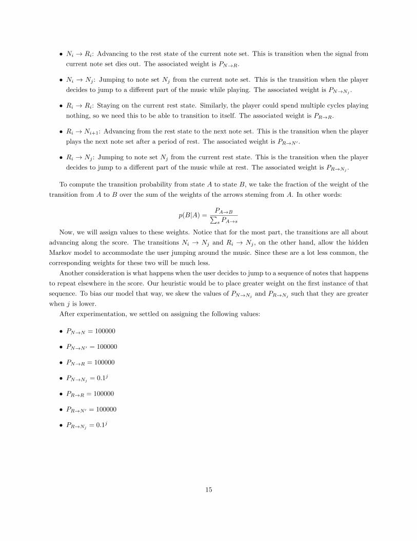
Figure 3.3 depicts a representative section of our hidden states. It shows arrows representing the transi-
tions from state to state, labeled with weights. The transition types and their descriptions are as follows:
• Ni → Ni: Staying on the current note set. Considering that we will be processing audio chunks many
times a second, the player will likely be holding out a note set for several cycles, so this transition
accounts for that. The associated weight is PN→N .
• Ni → Ni+1: Advancing from the current note set to the next note set. This is the transition when the
player plays the next note set. The associated weight is PN→N ′ .
14
• Ni → Ri: Advancing to the rest state of the current note set. This is transition when the signal from
current note set dies out. The associated weight is PN→R.
• Ni → Nj : Jumping to note set Nj from the current note set. This is the transition when the player
decides to jump to a different part of the music while playing. The associated weight is PN→Nj .
• Ri → Ri: Staying on the current rest state. Similarly, the player could spend multiple cycles playing
nothing, so we need this to be able to transition to itself. The associated weight is PR→R.
• Ri → Ni+1: Advancing from the rest state to the next note set. This is the transition when the player
plays the next note set after a period of rest. The associated weight is PR→N ′ .
• Ri → Nj : Jumping to note set Nj from the current rest state. This is the transition when the player
decides to jump to a different part of the music while at rest. The associated weight is PR→Nj .
To compute the transition probability from state A to state B, we take the fraction of the weight of the
transition from A to B over the sum of the weights of the arrows steming from A. In other words:
p(B|A) =PA→B∑s PA→s
Now, we will assign values to these weights. Notice that for the most part, the transitions are all about
advancing along the score. The transitions Ni → Nj and Ri → Nj , on the other hand, allow the hidden
Markov model to accommodate the user jumping around the music. Since these are a lot less common, the
corresponding weights for these two will be much less.
Another consideration is what happens when the user decides to jump to a sequence of notes that happens
to repeat elsewhere in the score. Our heuristic would be to place greater weight on the first instance of that
sequence. To bias our model that way, we skew the values of PN→Njand PR→Nj
such that they are greater
when j is lower.
After experimentation, we settled on assigning the following values:
• PN→N = 100000
• PN→N ′ = 100000
• PN→R = 100000
• PN→Nj= 0.1j
• PR→R = 100000
• PR→N ′ = 100000
• PR→Nj= 0.1j
15
3.3.1 Restricting Transitions by Page
In the context of a piece with multiple pages of sheet music, it is reasonable to believe that the player will
not suddenly decide to play notes that are more than a few measures before and after the visible page. As
such, we can adapt the transition probabilities accordingly.
Namely, if Si is more than a few measures before the end of the previous page, or is more than a few
measures after the start of the next page, we set the weight of all transitions pointing to Si to 0. In other
words, these states become considered unreachable. Note that these weight modifications are dependent on
which page is the current one, so when the page gets flipped (either automatically or by the player), we
restore the original weights, determine which states are now unreachable, and then zero out the transitions
to those states.
16
Chapter 4
Implementation
We implemented this algorithm in Java for the Android platform as part of a sheet music application. We
used the TarsosDSP library [12], which offered a clean framework for audio processing in Java. However,
TarsosDSP depends on some Java libraries (namely, javax libraries) that are not available in Android, so
we took out the components that depended on those unavailable libraries and reimplemented some of them
specifically for Android [11].
We chose to process the recorded audio at a sample rate of 44100 samples per second. The TarsosDSP
library lets us process real-time audio in chunks of any size we want, and we chose to process chunks of length
2048 samples, a value recommended by the TarsosDSP authors. The library also lets us set an overlap value,
which is the number of samples from the end of the current chunk to carry over to the beginning of the next
chunk. We chose an overlap value of 1024 samples, which was also recommended. Putting it all together,
we process chunks at a rate of 441002048−1024 ≈ 43 chunks per second. This rate is more than sufficient for piano
pieces, since it exceeds the the rate at which humans can even perceive separate notes.
Throughout our implementation, we aggressively strove to precompute anything we could, so that we
minimize the amount of work we perform at every chunk.
4.1 Goertzel Algorithm
To extract the frequency magnitudes from a chunk of audio samples, one might instinctively think to use the
fast Fourier transform algorithm, which extracts the discrete Fourier transform (DFT) coefficients for that
chunk. These coefficients, whose absolute value would be the magnitudes, correspond to frequencies that are
integer multiples of the fundamental frequency of the chunk. In our case of a sample rate of 44100 Hz and a
chunk size of 2048, these frequencies are 441002048 k ≈ 21.53k Hz, for k ∈ 0, 1, 2, . . . , 2047. However, few of these
frequencies closely match up to the observed frequencies that we are interested in.
We decided instead to use the Goertzel algorithm [7], which computes the DFT coefficient for just a single
frequency. A great property of this algorithm is that by carefully selecting parameters, we can finely home
in on the frequency that we want to analyze. Namely, given positive integers k and N , and the sampling
frequency fs, the algorithm yields the DFT coefficient for the frequency fskN Hz. Table A.1 lists the values
of k and N that we use for each observed frequency. For further discussion on how we chose these values,
17
see Appendix B.
We specifically use a version of the Goertzel algorithm that yields the power of the frequency, which is
the square of the coefficient’s magnitude. It is expressed as follows, where x is the array of sample values in
the audio chunk and sk is an intermediate array:
sk[n] = x[n] + 2 cos
(2πk
N
)sk[n− 1]− sk[n− 2]
|Xk|2 = sk[N − 1]2 − 2 cos
(2πk
N
)sk[n− 1]sk[n− 2] + sk[n− 2]2
We assume sk[−1] = sk[−2] = 0. After taking the square root of the second equation, we still need to
divide by N to normalize the magnitude. Thus, the final expression for the magnitude of the frequency is:√sk[N − 1]2 − 2 cos
(2πkN
)sk[n− 1]sk[n− 2] + sk[n− 2]2
N
Notice that in these expressions, we never use the value of k itself. Rather, the factor 2 cos(2πkN
)occurs
twice, so it is this value we actually store for each frequency instead of k.
Ultimately, for each of the 88 observed frequencies, we apply this algorithm with the frequency’s corre-
sponding k and N values, and putting that together gets us our magnitude vector for this audio chunk.
4.2 Preprocessing
When we load a music piece, we prepare several items.
First, we prepare our hidden states. If there were originally n note sets extracted from the score, then
after adding the rest states, we have a total of 2n hidden states: {S0, S1, S2, S3, . . . , S2n−1}Next, we prepare a confidence array c, which is a floating-point array whose length is 2n, the number
of hidden states we prepared above. Each value represents the probability that the corresponding state is
the current state. In other words, c[i] = p(St = Si|m1:t). This also means that at the end of each time
step, it should be the case that∑2n−1i=0 c[i] = 1. If the first and last states on the current page is Sa and Sb,
respectively, we set the initial values of the confidence array to be 1b−a+1 for c[i] where a ≤ i ≤ b.
Finally, for each of the hidden states Si, we precompute their unit vectors Si. Recall that this computation
involves the background noise vector b. To keep things simple, we assume a flat spectrum of background
noise at a pretty low volume, so we let b = 〈0.01, 0.01, 0.01, . . . , 0.01〉. This value should be small compared
to the harmonic strengths that we characterized earlier.
With these unit vectors precomputed, it will be fast to compute the function E we designed in Sec-
tion 3.2.2, since the dot product is the only thing that needs to be computed.
4.3 Main Loop
First, we take the chunk of audio and run it through the Goertzel algorithm to get our magnitude vector m.
Recall our modified version of the forward algorithm:
18
p(St|m1:t) ∝ E(mt, St)∑St−1
p(St|St−1)p(St−1|m1:t−1)
We compute the next version of the confidence array c′ for 0 ≤ i < 2n as follows:
c′[i] = E(m, Si)
2n−1∑j=0
p(Si|Sj)c[j]
After normalizing the values in c′ such that∑2n−1i=0 c′[i] = 1, we have our new c.
At the end of each time step, we also determine which original note set Ni has the highest total confidence.
Because of the associated rest state Ri, we add together their confidence values, which correspond to c[2i]
and c[2i + 1], respectively. If the note set with the highest total confidence exceeds some threshold, we
report that the player is indeed located at this note set and the UI should indicate as such. Otherwise, we
report that the player’s location is unknown. We experimented with different values and decided to set our
confidence threshold at 0.5. In the case that the note set we report is the last one on the page, we tell the
app to advance to the next page.
4.4 Restricting the Considered States
To follow up Section 3.3.1, we can restrict our loop if we know certain states will not get any confidence
because they are too far outside of the current page. Let Sa be the earliest state we think the user might
jump to (a few measures before the end of the previous page) and Sb be the latest (a few measures after the
start of the next page). Instead of looping i and j from 0 to 2n − 1, we can now instead loop from a to b.
That way, we only consider the note sets in the current page in addition to the couple around it.
This restriction has the nice benefit of making the algorithm more scalable in terms of the number of
pages in the piece. Normally, the processing complexity for one step in a hidden Markov model increases
with the square of the total number of possible hidden states. However, by applying this restriction, the
number of states we actually need to loop through is the number of note sets on the current page (in addition
to note sets in the extra few measures before and after the page). Regardless of how many other notes exist
in the rest of the piece, whether it is 20 or 2000, they are considered unreachable, so we do not need to
include them in the loop.
4.5 Results
We ran our application on a 2012 Nexus 7 tablet, running Android 4.4.2. As of this paper, the hardware is
slightly dated, but our score following algorithm performed with no perceptible latency.
We had two test pieces, Twinkle Twinkle Little Star, and Minuet in G by J.S. Bach. Both pieces were
two pages long. For each, we manually specified the sequence of note sets in the score. See Appendix C for
the full note set sequence of Minuet in G.
Our implementation works well for both pieces. When players played to the end of the first page, our app
advances to the second page automatically. Additionally, it works on various pianos with slightly different
19
timbres. Understandably, if the instrument the player is using is not a piano, it does not follow the player
as accurately, since the harmonic characteristics would be too different from the expected ones.
We found that the piano has to be fairly in tune for our algorithm to work well. If the piano is out of
tune by more than about 20 cents, the Goertzel algorithm can no longer reliably extract the magnitudes of
the observed frequencies.
A video of our application in action can be seen at [2].
20
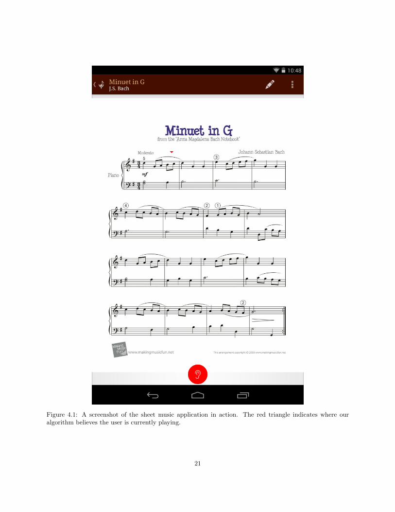
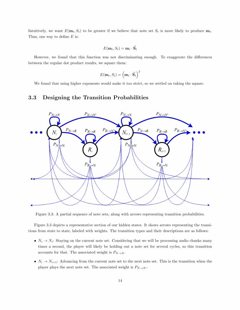
Figure 4.1: A screenshot of the sheet music application in action. The red triangle indicates where ouralgorithm believes the user is currently playing.
21
Chapter 5
Future Work
5.1 Understanding Tempo and Rhythm
In its current form, this algorithm is completely agnostic to tempo. If the player plays the notes completely
out of rhythm, as long as the notes are played in order, the algorithm does not really treat it any differently.
This also means that if the piece happens to have two phrases that happen to have the same note sequence,
but in a different rhythm, the algorithm still processes them the same way. This is because the resulting
note set sequences for both sections would be identical.
By annotating the note sets with their lengths (half a beat, two beats, etc.), we can start to incorporate
an understanding of how long we expect the note to be held. One approach could be to create a separate
mechanism that keeps track of how long the player has played each note set. Since we know the number of
beats each note set is supposed to last, we can estimate their current tempo, most likely with some sort of
smoothing.
Using this estimated tempo, we can vary the transition probabilities over time. For example, if the user
just started playing a new note set, the probability of staying on that note set is high while the probability of
advancing to the next one is low. Over time, as the note set is held out, these probabilities should gradually
be tipped the other way so after the expected amount of time, the probability of advancing to the next note
set becomes very high.
5.2 Extension to other Instruments
As described in Section 3.2.1, the harmonics of note produced by an instrument can characterize that
instrument’s sound. By determining the harmonic characteristics for other desired instruments, we can
tailor this algorithm for those as well.
This can also be implemented as a calibration process, where we have the user play a number of (possibly
predetermined) notes on their instrument. We can then analyze the magnitude vectors to understand that
instrument’s harmonic characteristics.
22
5.3 Better Note Break Detection
At the moment, when there is a sequence of repeating notes, the algorithm has trouble telling the notes
apart. Because the Ni → Ni and Ni → Ni+1 transitions lead to identical-looking states in such a sequence,
the forward algorithm will essentially cause the probability mass to rush towards the end of the repeated
note sets.
One possible approach is to see if the magnitude of the current magnitude vector is significantly larger
than that of the previous one. If so, that may indicate the onset of a new note being played. If we add this
notion to observed state, we can vary the transition probabilities as necessary.
Implementing Section 5.1 may also help this problem become less severe.
5.4 Additional Considerations for a Useful App
We developed this algorithm as a component of a sheet music application. In order for the app to be useful,
there are other issues we need to address other than just making it able to follow the user’s playing.
5.4.1 Importing Sheet Music
It should be easy and painless for a user to import their own sheet music. We did not have the resources
to implement this import flow in our app, and thus, had to manually put together the note set sequence for
the aforementioned pieces.
One of the standard formats for digital sheet music notation is MusicXML [3], which is an exportable
format on modern music notation software. In principle, we could read files in this format, extract the note
set sequence, and then render the pages of the score. A similar process could be done with files in ABC
notation [1], which is another text format for music notation.
We could even let the user import MIDI files. While MIDI files are generally devoid of notation, such as
the key, time signature, and staves, we can easily extract the sequence of notes. Then, we just render the
notes on a simple score in a basic manner. It may not look as neat, but it will probably be usable.
5.4.2 Pagination and Page Transitions
Currently, the pagination of the score is very cut and dried. The full sequence of note sets is broken up into
contiguous chunks as pages, and only one is visible at a time. While this made for a more straightforward
implementation, the user experience is not optimal. As they play and get towards the end of the page,
there is no way to preview the first notes on the next page without outright flipping the page themselves.
Arguably, physical sheet music is no different, and the usual “workaround” is to temporarily memorize the
last several measures of the current page and flip to the next one right then and there. However, since our
app is digital, we have a lot more freedom and power to experiment with interactions that are not possible
or very difficult on paper.
One simple way to reinvent the page flip is to present the score like a piano roll, as a single line of sheet
music that horizontally stretches as much as needed. Then, the sheet music continuously slides towards the
23
left as the user plays the piece. This can also be done vertically, presenting the score as a single, very tall
page that scrolls upward as the user plays.
Yet another way is to perform a “wipe” kind of transition. When the user approaches the end of the
page, the top of the page starts to peel away, revealing the top of the next page. Once the user reaches the
top of the next page, the rest of the original page peels away. This has the advantage where the notes never
move within the page.
With any of these techniques, we can still apply the transition restriction optimization we discuss in
Section 3.3.1, though it will not be as straightforward to implement. It is interesting to note that when
we suggested these alternative page transitions to users, many of them expressed an immediate rejection of
the idea. We hypothesize that this reaction may stem from years of familiarity with how they use physical
sheet music. It is worth conducting a proper usability study to see if users can get accustomed to the new
transitions and perhaps even prefer one over the regular page flip.
On a similar note, our implementation is currently hardcoded to advance the page only on the last note
of the page. Users have expressed their desire to be able to specify where in the score they would like the
page flip to happen, typically around two measures before the end of the page.
24
Chapter 6
Summary
In this paper, we have designed and implemented a hidden Markov model approach to follow a musician’s
location in a musical score, using only sound as input. We have demonstrated that by understanding
basic sheet music semantics and how instruments produce sound, we can carefully craft the states and the
probability distributions that we use in the hidden Markov model. Implementation-wise, we preprocess a
lot of components so that each iteration of the main loop can run more efficiently. Ultimately, we were able
to fully implement our algorithm in Java for Android devices, and it performed admirably on real pieces of
music. Finally, we present various directions we can pursue in the future to further improve the robustness
and accuracy of the algorithm.
25
Bibliography
[1] abc notation. http://abcnotation.com/.
[2] Final presentation. https://www.youtube.com/watch?v=itdyN98bzGI.
[3] Musicxml. http://www.musicxml.com/.
[4] Jonathan Aceituno. Real-time score following techniques.
[5] Andreas Arzt, Gerhard Widmer, and Simon Dixon. Automatic page turning for musicians via real-time
machine listening. In ECAI, pages 241–245, 2008.
[6] Simon Dixon. An on-line time warping algorithm for tracking musical performances.
[7] Gerald Goertzel. An algorithm for the evaluation of finite trigonometric series. American mathematical
monthly, pages 34–35, 1958.
[8] Bryan Pardo and William Birmingham. Modeling form for on-line following of musical performances.
In PROCEEDINGS OF THE NATIONAL CONFERENCE ON ARTIFICIAL INTELLIGENCE, vol-
ume 20, page 1018. Menlo Park, CA; Cambridge, MA; London; AAAI Press; MIT Press; 1999, 2005.
[9] Christopher Raphael. Automatic segmentation of acoustic musical signals using hidden markov models.
Pattern Analysis and Machine Intelligence, IEEE Transactions on, 21(4):360–370, 1999.
[10] Christopher Raphael. A hybrid graphical model for aligning polyphonic audio with musical scores. In
ISMIR. Citeseer, 2004.
[11] Steve Rubin and Andrew Lee. TarsosDSP. https://github.com/srubin/TarsosDSP, 2014.
[12] Joren Six, Olmo Cornelis, and Marc Leman. Tarsosdsp, a real-time audio processing framework in java.
In Audio Engineering Society Conference: 53rd International Conference: Semantic Audio, Jan 2014.
26
Appendix A
Observed Frequencies Table
NoteIndex
NoteName
Frequency(Hz)
Goertzel Parameters Harmonic Magnitudes
k N h1 h2 h3 h4 h5 h6
0 A0 27.500 1 1604 0.00 0.00 5.27 1.12 6.04 4.68
1 A]0/B[0 29.135 1 1514 0.00 0.01 5.86 1.31 5.84 4.57
2 B0 30.868 1 1429 0.00 0.02 6.45 1.52 5.65 4.45
3 C1 32.703 1 1348 0.00 0.04 7.00 1.74 5.45 4.32
4 C]1/D[1 34.648 1 1273 0.00 0.08 7.53 1.96 5.24 4.19
5 D1 36.708 1 1201 0.00 0.14 8.02 2.20 5.04 4.05
6 D]1/E[1 38.891 1 1134 0.01 0.24 8.46 2.44 4.83 3.91
7 E1 41.203 1 1070 0.01 0.40 8.85 2.69 4.63 3.77
8 F1 43.654 2 2020 0.02 0.62 9.19 2.93 4.42 3.62
9 F]1/G[1 46.249 2 1907 0.03 0.94 9.46 3.17 4.22 3.47
10 G1 48.999 2 1800 0.05 1.37 9.68 3.41 4.02 3.32
11 G]1/A[1 51.913 2 1699 0.07 1.93 9.83 3.64 3.83 3.18
12 A1 55.000 2 1604 0.10 2.65 9.92 3.85 3.64 3.03
13 A]1/B[1 58.270 2 1514 0.15 3.54 9.94 4.06 3.45 2.88
14 B1 61.735 2 1429 0.21 4.61 9.91 4.25 3.27 2.74
15 C2 65.406 3 2023 0.29 5.85 9.82 4.42 3.10 2.60
16 C]2/D[2 69.296 3 1909 0.39 7.26 9.69 4.57 2.93 2.46
17 D2 73.416 3 1802 0.53 8.82 9.50 4.71 2.76 2.33
18 D]2/E[2 77.782 3 1701 0.70 10.50 9.27 4.82 2.60 2.20
19 E2 82.407 3 1605 0.90 12.26 9.00 4.91 2.45 2.07
20 F2 87.307 4 2020 1.16 14.05 8.70 4.98 2.31 1.95
21 F]2/G[2 92.499 4 1907 1.47 15.82 8.37 5.03 2.17 1.83
22 G2 97.999 4 1800 1.83 17.51 8.02 5.05 2.03 1.72
23 G]2/A[2 103.826 4 1699 2.26 19.08 7.65 5.06 1.90 1.61
Continued on next page
27
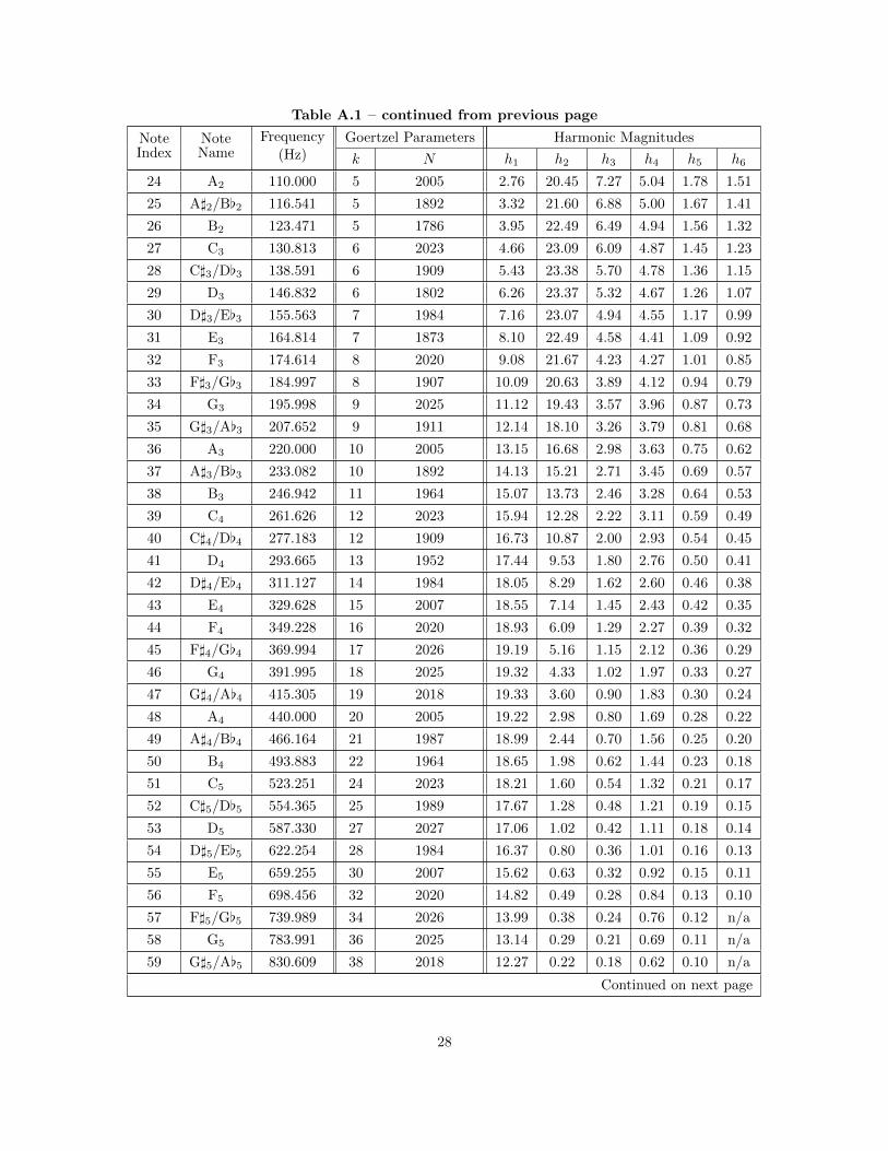
Table A.1 – continued from previous page
NoteIndex
NoteName
Frequency(Hz)
Goertzel Parameters Harmonic Magnitudes
k N h1 h2 h3 h4 h5 h6
24 A2 110.000 5 2005 2.76 20.45 7.27 5.04 1.78 1.51
25 A]2/B[2 116.541 5 1892 3.32 21.60 6.88 5.00 1.67 1.41
26 B2 123.471 5 1786 3.95 22.49 6.49 4.94 1.56 1.32
27 C3 130.813 6 2023 4.66 23.09 6.09 4.87 1.45 1.23
28 C]3/D[3 138.591 6 1909 5.43 23.38 5.70 4.78 1.36 1.15
29 D3 146.832 6 1802 6.26 23.37 5.32 4.67 1.26 1.07
30 D]3/E[3 155.563 7 1984 7.16 23.07 4.94 4.55 1.17 0.99
31 E3 164.814 7 1873 8.10 22.49 4.58 4.41 1.09 0.92
32 F3 174.614 8 2020 9.08 21.67 4.23 4.27 1.01 0.85
33 F]3/G[3 184.997 8 1907 10.09 20.63 3.89 4.12 0.94 0.79
34 G3 195.998 9 2025 11.12 19.43 3.57 3.96 0.87 0.73
35 G]3/A[3 207.652 9 1911 12.14 18.10 3.26 3.79 0.81 0.68
36 A3 220.000 10 2005 13.15 16.68 2.98 3.63 0.75 0.62
37 A]3/B[3 233.082 10 1892 14.13 15.21 2.71 3.45 0.69 0.57
38 B3 246.942 11 1964 15.07 13.73 2.46 3.28 0.64 0.53
39 C4 261.626 12 2023 15.94 12.28 2.22 3.11 0.59 0.49
40 C]4/D[4 277.183 12 1909 16.73 10.87 2.00 2.93 0.54 0.45
41 D4 293.665 13 1952 17.44 9.53 1.80 2.76 0.50 0.41
42 D]4/E[4 311.127 14 1984 18.05 8.29 1.62 2.60 0.46 0.38
43 E4 329.628 15 2007 18.55 7.14 1.45 2.43 0.42 0.35
44 F4 349.228 16 2020 18.93 6.09 1.29 2.27 0.39 0.32
45 F]4/G[4 369.994 17 2026 19.19 5.16 1.15 2.12 0.36 0.29
46 G4 391.995 18 2025 19.32 4.33 1.02 1.97 0.33 0.27
47 G]4/A[4 415.305 19 2018 19.33 3.60 0.90 1.83 0.30 0.24
48 A4 440.000 20 2005 19.22 2.98 0.80 1.69 0.28 0.22
49 A]4/B[4 466.164 21 1987 18.99 2.44 0.70 1.56 0.25 0.20
50 B4 493.883 22 1964 18.65 1.98 0.62 1.44 0.23 0.18
51 C5 523.251 24 2023 18.21 1.60 0.54 1.32 0.21 0.17
52 C]5/D[5 554.365 25 1989 17.67 1.28 0.48 1.21 0.19 0.15
53 D5 587.330 27 2027 17.06 1.02 0.42 1.11 0.18 0.14
54 D]5/E[5 622.254 28 1984 16.37 0.80 0.36 1.01 0.16 0.13
55 E5 659.255 30 2007 15.62 0.63 0.32 0.92 0.15 0.11
56 F5 698.456 32 2020 14.82 0.49 0.28 0.84 0.13 0.10
57 F]5/G[5 739.989 34 2026 13.99 0.38 0.24 0.76 0.12 n/a
58 G5 783.991 36 2025 13.14 0.29 0.21 0.69 0.11 n/a
59 G]5/A[5 830.609 38 2018 12.27 0.22 0.18 0.62 0.10 n/a
Continued on next page
28
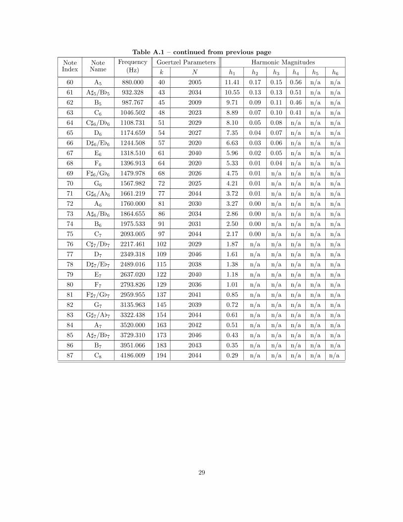
Table A.1 – continued from previous page
NoteIndex
NoteName
Frequency(Hz)
Goertzel Parameters Harmonic Magnitudes
k N h1 h2 h3 h4 h5 h6
60 A5 880.000 40 2005 11.41 0.17 0.15 0.56 n/a n/a
61 A]5/B[5 932.328 43 2034 10.55 0.13 0.13 0.51 n/a n/a
62 B5 987.767 45 2009 9.71 0.09 0.11 0.46 n/a n/a
63 C6 1046.502 48 2023 8.89 0.07 0.10 0.41 n/a n/a
64 C]6/D[6 1108.731 51 2029 8.10 0.05 0.08 n/a n/a n/a
65 D6 1174.659 54 2027 7.35 0.04 0.07 n/a n/a n/a
66 D]6/E[6 1244.508 57 2020 6.63 0.03 0.06 n/a n/a n/a
67 E6 1318.510 61 2040 5.96 0.02 0.05 n/a n/a n/a
68 F6 1396.913 64 2020 5.33 0.01 0.04 n/a n/a n/a
69 F]6/G[6 1479.978 68 2026 4.75 0.01 n/a n/a n/a n/a
70 G6 1567.982 72 2025 4.21 0.01 n/a n/a n/a n/a
71 G]6/A[6 1661.219 77 2044 3.72 0.01 n/a n/a n/a n/a
72 A6 1760.000 81 2030 3.27 0.00 n/a n/a n/a n/a
73 A]6/B[6 1864.655 86 2034 2.86 0.00 n/a n/a n/a n/a
74 B6 1975.533 91 2031 2.50 0.00 n/a n/a n/a n/a
75 C7 2093.005 97 2044 2.17 0.00 n/a n/a n/a n/a
76 C]7/D[7 2217.461 102 2029 1.87 n/a n/a n/a n/a n/a
77 D7 2349.318 109 2046 1.61 n/a n/a n/a n/a n/a
78 D]7/E[7 2489.016 115 2038 1.38 n/a n/a n/a n/a n/a
79 E7 2637.020 122 2040 1.18 n/a n/a n/a n/a n/a
80 F7 2793.826 129 2036 1.01 n/a n/a n/a n/a n/a
81 F]7/G[7 2959.955 137 2041 0.85 n/a n/a n/a n/a n/a
82 G7 3135.963 145 2039 0.72 n/a n/a n/a n/a n/a
83 G]7/A[7 3322.438 154 2044 0.61 n/a n/a n/a n/a n/a
84 A7 3520.000 163 2042 0.51 n/a n/a n/a n/a n/a
85 A]7/B[7 3729.310 173 2046 0.43 n/a n/a n/a n/a n/a
86 B7 3951.066 183 2043 0.35 n/a n/a n/a n/a n/a
87 C8 4186.009 194 2044 0.29 n/a n/a n/a n/a n/a
29
Appendix B
Computing N and k for each
Observed Frequency
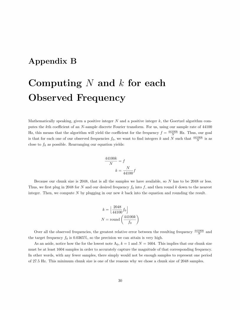
Mathematically speaking, given a positive integer N and a positive integer k, the Goertzel algorithm com-
putes the kth coefficient of an N -sample discrete Fourier transform. For us, using our sample rate of 44100
Hz, this means that the algorithm will yield the coefficient for the frequency f = 44100kN Hz. Thus, our goal
is that for each one of our observed frequencies f0, we want to find integers k and N such that 44100kN is as
close to f0 as possible. Rearranging our equation yields:
44100k
N= f
k =N
44100f
Because our chunk size is 2048, that is all the samples we have available, so N has to be 2048 or less.
Thus, we first plug in 2048 for N and our desired frequency f0 into f , and then round k down to the nearest
integer. Then, we compute N by plugging in our new k back into the equation and rounding the result.
k =⌊ 2048
44100f0
⌋N = round
(44100k
f0
)Over all the observed frequencies, the greatest relative error between the resulting frequency 44100k
N and
the target frequency f0 is 0.0365%, so the precision we can attain is very high.
As an aside, notice how the for the lowest note A0, k = 1 and N = 1604. This implies that our chunk size
must be at least 1604 samples in order to accurately capture the magnitude of that corresponding frequency.
In other words, with any fewer samples, there simply would not be enough samples to represent one period
of 27.5 Hz. This minimum chunk size is one of the reasons why we chose a chunk size of 2048 samples.
30
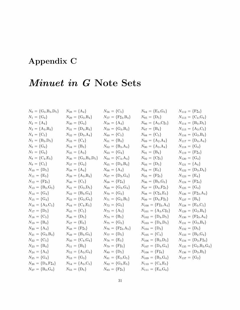
Appendix C
Minuet in G Note Sets
N0 = {G3,B3,D5}N1 = {G4}N2 = {A4}N3 = {A3,B4}N4 = {C5}N5 = {B3,D5}N6 = {G4}N7 = {G4}N8 = {C4,E5}N9 = {C5}N10 = {D5}N11 = {E5}N12 = {F]5}N13 = {B3,G5}N14 = {G4}N15 = {G4}N16 = {A3,C5}N17 = {D5}N18 = {C5}N19 = {B4}N20 = {A4}N21 = {G3,B4}N22 = {C5}N23 = {B4}N24 = {A4}N25 = {G4}N26 = {D4,F]4}N27 = {B3,G4}
N28 = {A4}N29 = {G3,B4}N30 = {G4}N31 = {D4,B4}N32 = {D3,A4}N33 = {C4}N34 = {B3}N35 = {A3}N36 = {G3,B3,D5}N37 = {G4}N38 = {A4}N39 = {A3,B4}N40 = {C5}N41 = {G3,D5}N42 = {B3,G4}N43 = {G3,G4}N44 = {C4,E5}N45 = {C5}N46 = {D5}N47 = {E5}N48 = {F]5}N49 = {B3,G5}N50 = {C4,G4}N51 = {B3}N52 = {A3,G4}N53 = {G3}N54 = {A3,C5}N55 = {D5}
N56 = {C5}N57 = {F]3,B4}N58 = {A4}N59 = {G3,B4}N60 = {C5}N61 = {B4}N62 = {B3,A4}N63 = {G4}N64 = {C4,A4}N65 = {D4,B4}N66 = {A4}N67 = {D3,G4}N68 = {F]4}N69 = {G3,G4}N70 = {G2}N71 = {G3,B5}N72 = {G5}N73 = {A5}N74 = {B5}N75 = {G5}N76 = {F]3,A5}N77 = {D5}N78 = {E5}N79 = {F]5}N80 = {D5}N81 = {E3,G5}N82 = {G3,E5}N83 = {F]5}
N84 = {E3,G5}N85 = {D5}N86 = {A3,C]5}N87 = {B4}N88 = {C5}N89 = {A2,A4}N90 = {A3,A4}N91 = {B4}N92 = {C]5}N93 = {D5}N94 = {E5}N95 = {F]5}N96 = {B3,G5}N97 = {D4,F]5}N98 = {C]4,E5}N99 = {D4,F]5}N100 = {F]3,A4}N101 = {A3,C]5}N102 = {D4,D5}N103 = {D4,D5}N104 = {D3}N105 = {C4}N106 = {B3,D5}N107 = {D4,G4}N108 = {F]4}N109 = {B3,G4}N110 = {C4,E5}N111 = {E4,G4}
N112 = {F]4}N113 = {C4,G4}N114 = {B3,D5}N115 = {A3,C5}N116 = {G3,B4}N117 = {D4,A4}N118 = {G4}N119 = {F]4}N120 = {G4}N121 = {A4}N122 = {D3,D4}N123 = {E4}N124 = {F]4}N125 = {G4}N126 = {F]3,A4}N127 = {B4}N128 = {E3,C5}N129 = {G3,B4}N130 = {F]3,A4}N131 = {G3,B4}N132 = {D5}N133 = {B2,G4}N134 = {D3,F]4}N135 = {G3,B3,G4}N136 = {D3,B3}N137 = {G2}
31