Real-time Machine Learning for Assistive Medical...

Real-time Machine Learning for Assistive Medical Robotics

Patrick M. Pilarski

Reinforcement Learning & Artificial Intelligence LaboratoryAlberta Innovates Centre for Machine Learning

Dept. Computing Science, University of AlbertaEdmonton, Alberta, Canada

Chiba University, Nov. 18, 2011

Outline

‣ The University of Alberta

‣ Toward Intelligent Artificial Limbs

‣ Reinforcement Learning

‣ Real-time Prediction in a Clinical Setting(General Value Functions & Nexting)

‣ Results (Able-bodied & Clinical)

2

Edmonton

4

CS Grad Studies at U. of Alberta, October, 2006© 2006 R. C. Holte, AICML

Alberta Nature

7


• Opened in 1908

• 6,000 Graduate students

• 30,000 Undergraduate students

• 1 of the top 100 universities in the world

8

The University of Alberta


Department of Computing Science University of Alberta

9

Reinforcement Learning & Artificial Intelligence LabPIs: Rich Sutton, Csaba SzepesvariMichael Bowling, Dale Schuurmans

10

Outline






11

Multifunction Myoelectric Prostheses

Otto Bock’s Dynamic Arm combined with myoelectric wrist rotator and prehensor.

(Image: Otto Bock; Schematic: Dawson, Ph.D. Thesis, 2011.)

Three Known Barriers

“Three main problems were mentioned as reasons that amputees stop using their ME prostheses: nonintuitive control, lack of sufficient feedback, and insufficient functionality.”

— Peerdeman et al., JRRD, 2011.

13

MyoHand VariPlus SpeedHand Image: Otto Bock

Intelligent Interfaces(Prostheses that approach and someday exceed

the abilites of a biological limb.)

14

DLR Hand Arm System Image: German Aerospace Center (DLR) & IEEE Spectrum

?

Intelligent Interfaces(Prostheses that approach and someday exceed

the abilites of a biological limb.)

15

http://spectrum.ieee.org/tag/dlr


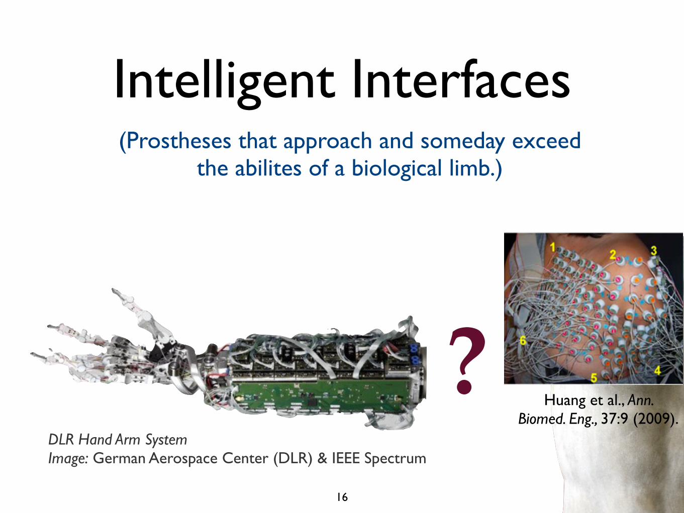
Intelligent Interfaces


?Huang et al., Ann.

Biomed. Eng., 37:9 (2009).

(Prostheses that approach and someday exceed the abilites of a biological limb.)

16



MACHINELEARNING

SYSTEM


Machine LearningIn the face of growing complexity, learn the correct

way to map numerous EMG signals to actuator commands.

17

SIGNALS



• Excellent examples of machine learning work in classifying EMG patterns for use in limb control (e.g. Oskoei and Hu ‘08, Parker et al. ‘06, Sensinger et al. ’09).

• However, most contemporary learning approaches rely on external knowledge of their domain to guide learning, and function primarily in offline or batch learning scenarios.

• This breaks down as the complexity and individuality of the input and output space increases; very hard to determine the “correct” thing to do.

State of the Art

18

Three Missing Elements• Real-time machine learning.

(Online, adaptive algorithms; noted by Sensinger et al. ’09, Scheme & Englehart ‘11)

• Generalized interfaces.(Blank-slate human-machine interaction & collaboration; e.g. Pilarski et al. 2011)

• Data-respecting biomedical pattern analysis.(Complexity is good: interpreting myriad signals without reducing the sensorimotor space)

19

Ongoing Projects

• Real-time control learning without a priori information about a user or device.

• Prediction and anticipation of signals during patient-device interaction.

• Collaborative algorithms for the online human improvement of limb controllers.

20

Team• RLAI / AICML: new methods for improved

control, feedback, and online interaction.

• Mec. Eng.: new mechanical limbs and platforms for amputee training (MTT).

• Glenrose / Medicine: new surgeries (TMR & TSR), patients, and clinical expertise.

21

Setting: TMR/TSR

22

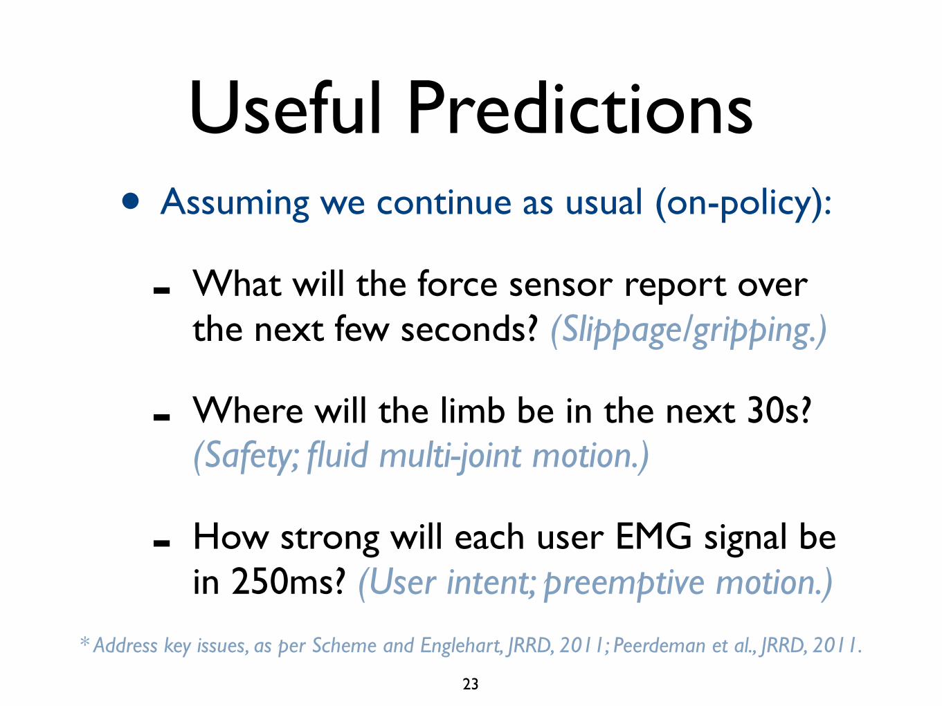
Useful Predictions• Assuming we continue as usual (on-policy):

- What will the force sensor report over the next few seconds? (Slippage/gripping.)

- Where will the limb be in the next 30s? (Safety; fluid multi-joint motion.)

- How strong will each user EMG signal be in 250ms? (User intent; preemptive motion.)

* Address key issues, as per Scheme and Englehart, JRRD, 2011; Peerdeman et al., JRRD, 2011. 23

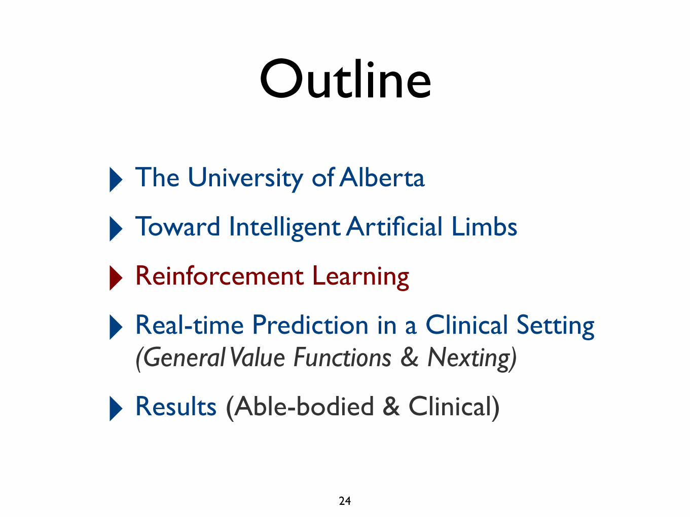
Outline






24

25 Sutton and Barto, MIT Press (1998)

Reinforcement Learning is an approach to:• Natural intelligence

• Artificial intelligence

• Optimal control

• Operations research

• Solving partially observable Markov decision processes

(and the perspective that all of these are the same)

26 Slide content thanks to Rich Sutton

Main Ideas• Reinforcement learning involves an agent

and an environment.

• The learning system (agent) perceives the state of the environment via a set of observations and takes actions.

• It then receives a new set of observations and a reward.

• These observations and rewards are used to predict future rewards, and to change the agent’s policy (how it selects actions).

• Key point: A single, scalar reward signal drives learning.

27

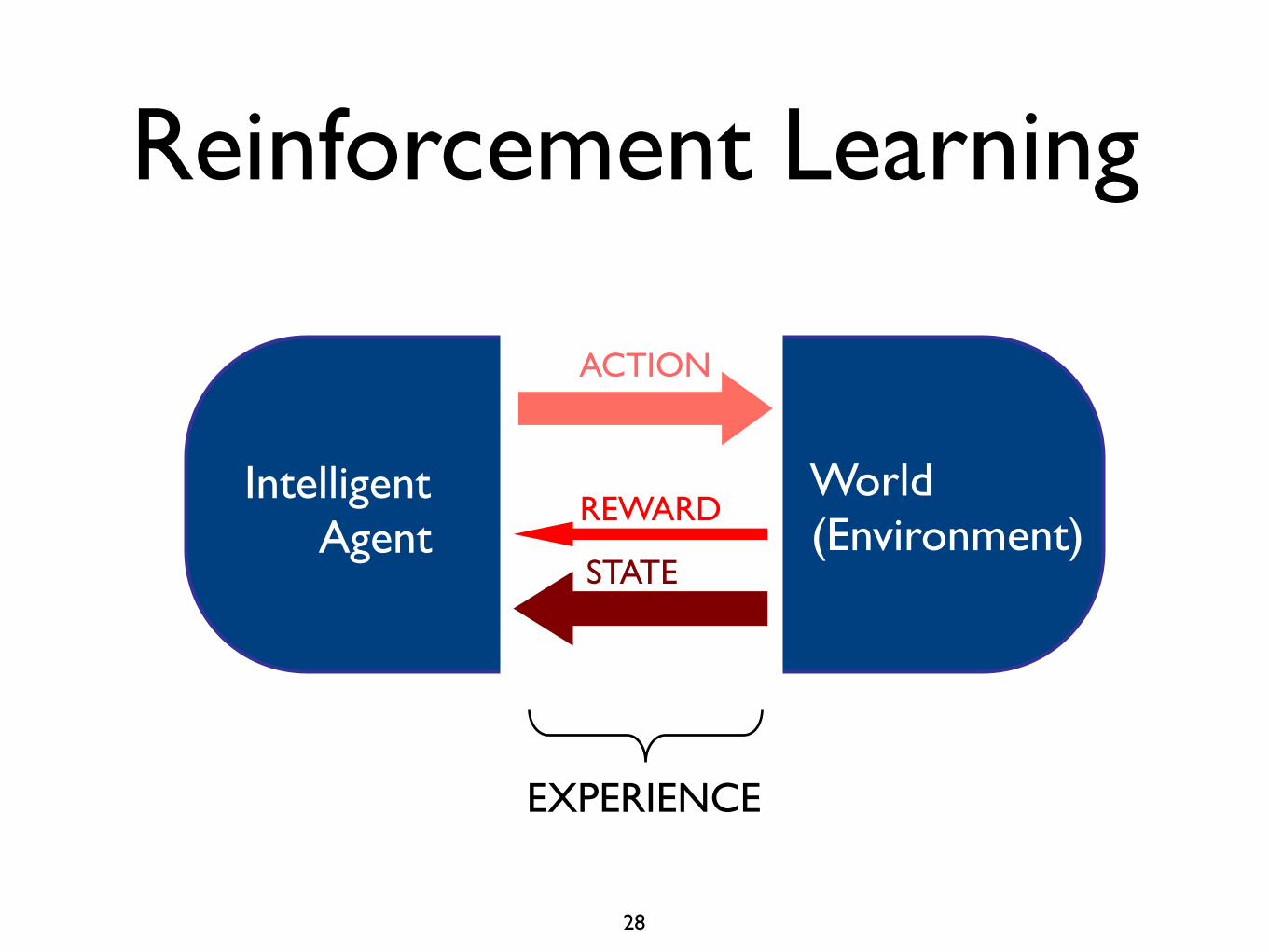
ACTION

STATE

REWARD

EXPERIENCE

Reinforcement Learning

IntelligentAgent

World(Environment)

28

0

1000

2000

3000

4000

1983 1988 1993 1998 2003 2008

Google scholar hits for the phrase“reinforcement

learning”

Number RL Papers per Year

Slide content thanks to Rich Sutton29

RL Headlines

• RL is widely used in robotics

• RL algorithms have found the best known approximate solutions to many games(RL is part of the revolution in solving Go)

• RL algorithms are now the standard model of reward processing in the brain

• RL breaks the curse of dimensionality


What is Special About RL?

• Radical generality

• None of the signals are given any interpretation... no reference signals or labels... no human interpretation, no calibration

• Just data in the form of signals... one of which is to be maximized (reward)


Outline






32

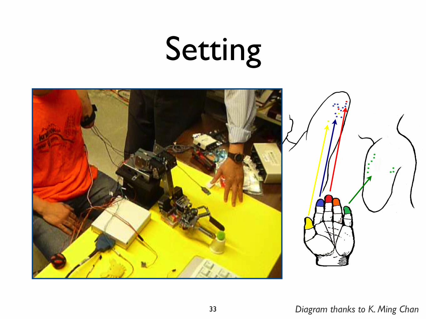
Setting

33 Diagram thanks to K. Ming Chan

Useful Predictions• Assuming we continue as usual (on-policy):

- What will the force sensor report over the next few seconds? (Slippage/gripping.)

- Where will the limb be in the next 30s? (Safety; fluid multi-joint motion.)

- How strong will each user EMG signal be in 250ms? (User intent; preemptive motion.)

* Address key issues, as per Scheme and Englehart, JRRD, 2011; Peerdeman et al., JRRD, 2011. 34

Online Nexting• General Value Functions.

(Sutton et al., 2011, AAMAS)

• GVFs form questions; “what will happen next?” (Nexting)

• In brief: instead of reward, learn anticipations (expectations of real-valued signals).

• Can learn many temporally extended predictions in parallel.

35

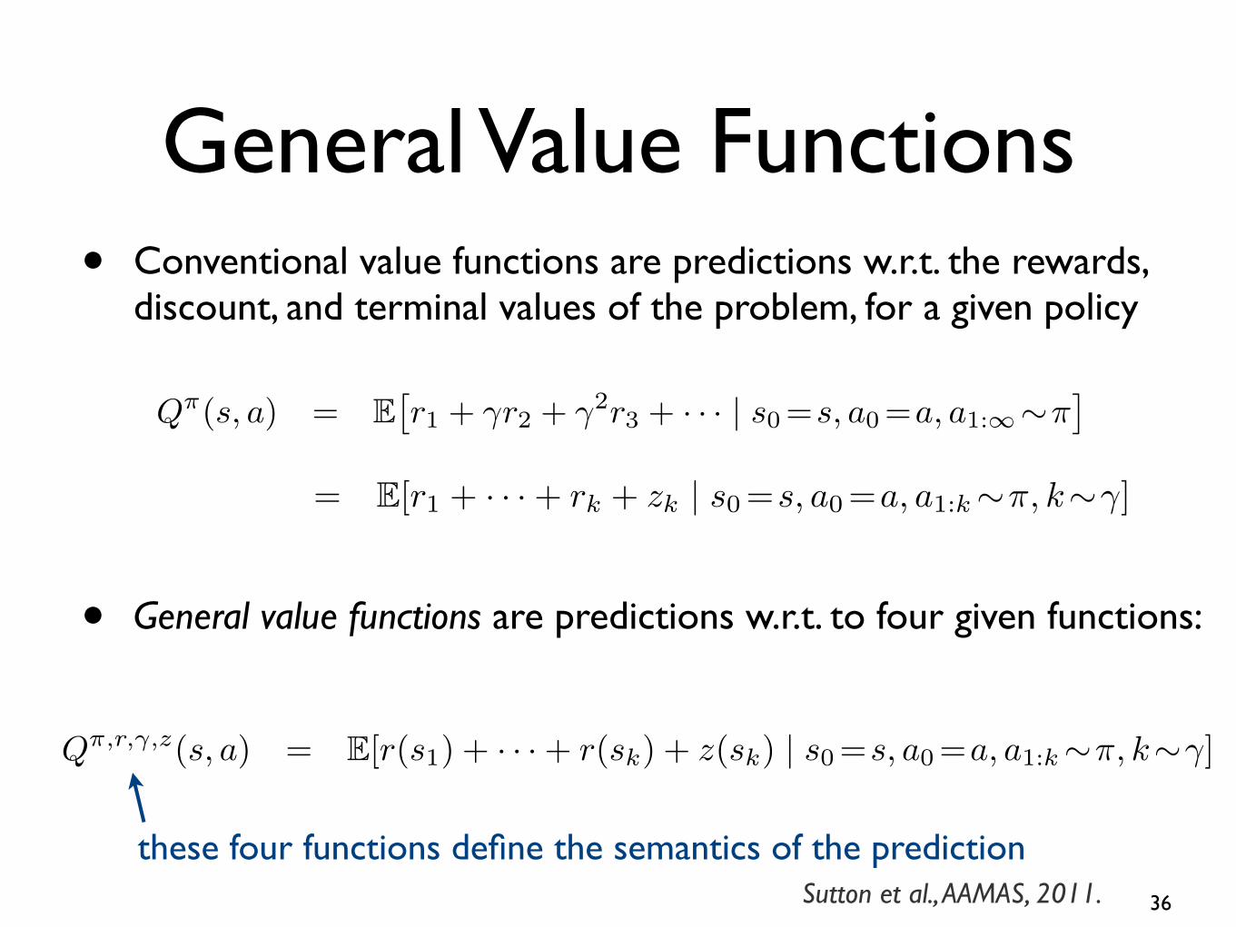
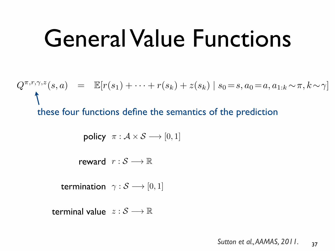
General Value Functions• Conventional value functions are predictions w.r.t. the rewards,

discount, and terminal values of the problem, for a given policy

• General value functions are predictions w.r.t. to four given functions:

Qπ(s, a) = E�r1 + γr2 + γ2r3 + · · · | s0=s, a0=a, a1:∞∼π

�

Qπ(s, a) = E[r1 + · · ·+ rk + zk | s0=s, a0=a, a1:k∼π, k∼γ]

Qπ,r,γ,z(s, a) = E[r(s1) + · · ·+ r(sk) + z(sk) | s0=s, a0=a, a1:k∼π, k∼γ]

Qπ,r,γ,z(s, a) =�

s�

P (s�|s, a)�r(s�) + γ(s�)

�

a�

π(a�|s�)Qπ,r,γ,z(s�, a�) + (1− γ(s�))z(s�)

�

δ(s, a, s�; Q̂) = r(s�) + γ(s�)�

a�

π(a�|s�)Q̂(s�, a�) + (1− γ(s�))z(s�)− Q̂(s, a)

δt = r(st+1) + γ(st+1)�

a�

π(a�|st+1)Q̂(st+1, a�) + (1− γ(st+1))z(st+1)− Q̂(s, a)

2


�




s�

P (s�|s, a)�r(s�) + γ(s�)

�

a�

π(a�|s�)Qπ,r,γ,z(s�, a�) + (1− γ(s�))z(s�)

�

δ(s, a, s�; Q̂) = r(s�) + γ(s�)�

a�

π(a�|s�)Q̂(s�, a�) + (1− γ(s�))z(s�)− Q̂(s, a)

δt = r(st+1) + γ(st+1)�

a�


2


�




s�

P (s�|s, a)�r(s�) + γ(s�)

�

a�

π(a�|s�)Qπ,r,γ,z(s�, a�) + (1− γ(s�))z(s�)

�

δ(s, a, s�; Q̂) = r(s�) + γ(s�)�

a�

π(a�|s�)Q̂(s�, a�) + (1− γ(s�))z(s�)− Q̂(s, a)

δt = r(st+1) + γ(st+1)�

a�


2

these four functions define the semantics of the prediction36Sutton et al., AAMAS, 2011.

General Value FunctionsQπ(s, a) = E�r1 + γr2 + γ2r3 + · · · | s0=s, a0=a, a1:∞∼π

�




s�

P (s�|s, a)�r(s�) + γ(s�)

�

a�

π(a�|s�)Qπ,r,γ,z(s�, a�) + (1− γ(s�))z(s�)

�

δ(s, a, s�; Q̂) = r(s�) + γ(s�)�

a�

π(a�|s�)Q̂(s�, a�) + (1− γ(s�))z(s�)− Q̂(s, a)

δt = r(st+1) + γ(st+1)�

a�


2

these four functions define the semantics of the prediction

policy

reward

termination

terminal value


�




s�

P (s�|s, a)�r(s�) + γ(s�)

�

a�

π(a�|s�)Qπ,r,γ,z(s�, a�) + (1− γ(s�))z(s�)

�

δ(s, a, s�; Q̂) = r(s�) + γ(s�)�

a�

π(a�|s�)Q̂(s�, a�) + (1− γ(s�))z(s�)− Q̂(s, a)

δt = r(st+1) + γ(st+1)�

a�


π : A× S −→ [0, 1]

r : S −→ R

γ : S −→ [0, 1]

z : S −→ R

2

37Sutton et al., AAMAS, 2011.

Why GVFs?

• Thousands of accurate predictions can be made and learned in real time (i.e., 10hz)

• A single state representation be used to accurately predict many different sensors at many different time scales.

• A model-free algorithm that can learn fast enough to be useful.

Sutton et al., AAMAS, 2011.38

CONTROL ROBOTHUMAN

EMGSIGNALS

ACTUATORSIGNALS

CONTROL SIGNALS

. . .

FXN APP

GVF 1 GVF 2 GVF NGVF 3

STATE

P1 P2 P3 PN

FEEDBACK SIGNALS

Massively Parallel Prediction

39

• Where each prediction has its ownreward and discount rate

• Ideal predictions are the convolution of the reward with an exponential kernel

Predictions (Nexting)


�

V π(s) = E�r1 + γr2 + γ2r3 + · · · | s0=s, a0:∞∼π

�

s ∈ Sat ∈ Art ∈ R

γ ∈ [0, 1]

π : A× S −→ [0, 1]

ri

pit = f�t wi =6062�

j

ft(j)wi(j) ≈ rit+1 + γirit+2 + (γi)2rit+3 + (γi)3rit+4 + · · ·

wit+1 = wi

t + α�rit+1 + γif�t+1wi

t − f�t wit

�eit

eit = γiλeit−1 + ft

δit = rit+1 + γif�t+1wit − f�t wi

t

Linear approximation of state–action values:

Qπ(s, a) ≈ w�f(s, a) = Q̂(s, a)

Q̂(s, a) = w�f(s, a) ≈ Qπ,r,γ,z(s, a)

Sarsa:

∆wt = αδtf(st, at)

δt = rt+1 + γQ̂(st+1, at+1)− Q̂(st, at)

1


�

V π(s) = E�r1 + γr2 + γ2r3 + · · · | s0=s, a0:∞∼π

�


γ ∈ [0, 1]

π : A× S −→ [0, 1]

ritγi ∈ [0, 1)

pit = f�t wi =6062�

j


wit+1 = wi


t − f�t wit

�eit



t


Qπ(s, a) ≈ w�f(s, a) = Q̂(s, a)

Q̂(s, a) = w�f(s, a) ≈ Qπ,r,γ,z(s, a)

Sarsa:



1


�

V π(s) = E�r1 + γr2 + γ2r3 + · · · | s0=s, a0:∞∼π

�


γ ∈ [0, 1]

π : A× S −→ [0, 1]

ritγi ∈ [0, 1)

pit = f�t wi =6062�

j


wit+1 = wi


t − f�t wit

�eit



t


Qπ(s, a) ≈ w�f(s, a) = Q̂(s, a)

Q̂(s, a) = w�f(s, a) ≈ Qπ,r,γ,z(s, a)

Sarsa:



1

40

Learning GVFs

• Temporal-Difference (TD) learning

• Linear TD(λ) (Sutton, 1988)


�

V π(s) = E�r1 + γr2 + γ2r3 + · · · | s0=s, a0:∞∼π

�


γ ∈ [0, 1]

π : A× S −→ [0, 1]

pi = f�wi

wit+1 = wi


t − f�t wit

�eit



t


Qπ(s, a) ≈ w�f(s, a) = Q̂(s, a)

Q̂(s, a) = w�f(s, a) ≈ Qπ,r,γ,z(s, a)

Sarsa:



Expected Sarsa:

δt = rt+1 + γ�

a

π(a|st+1)Q̂(st+1, a)− Q̂(st, at)

1

just ft if λ=0

Outline






42

Able-Bodied Study

• Eight runs at 5–10 min (12k–25k timesteps).

• Record EMG signals and joint angles.

• Recording and learning at 40Hz.

• GVF state = TileCoder(8,10) {C-EMG x 2, elbow joint angle, wrist joint angle}.

43

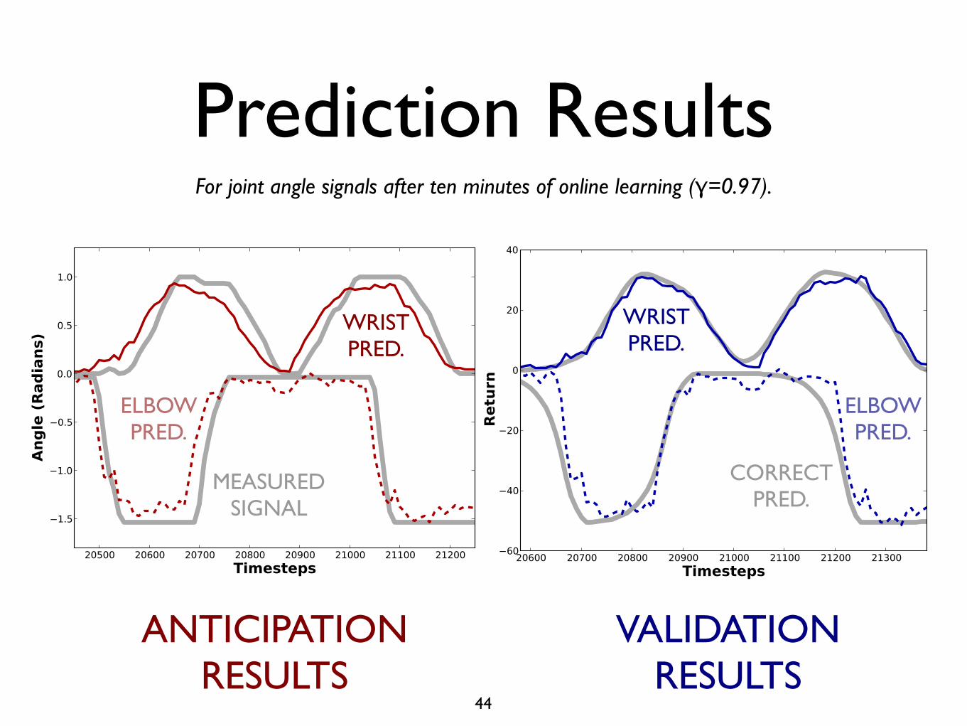
Prediction Results

44

For joint angle signals after ten minutes of online learning (γ=0.97).

ELBOWPRED.

WRISTPRED.

WRISTPRED.

ELBOWPRED.

ANTICIPATIONRESULTS

VALIDATIONRESULTS

MEASUREDSIGNAL

CORRECTPRED.

Prediction Results

45

For EMG signals after ten minutes of online learning (γ=0.97).

PRED.PRED.

ANTICIPATIONRESULTS

VALIDATIONRESULTS

MEASUREDSIGNAL

CORRECTPRED.

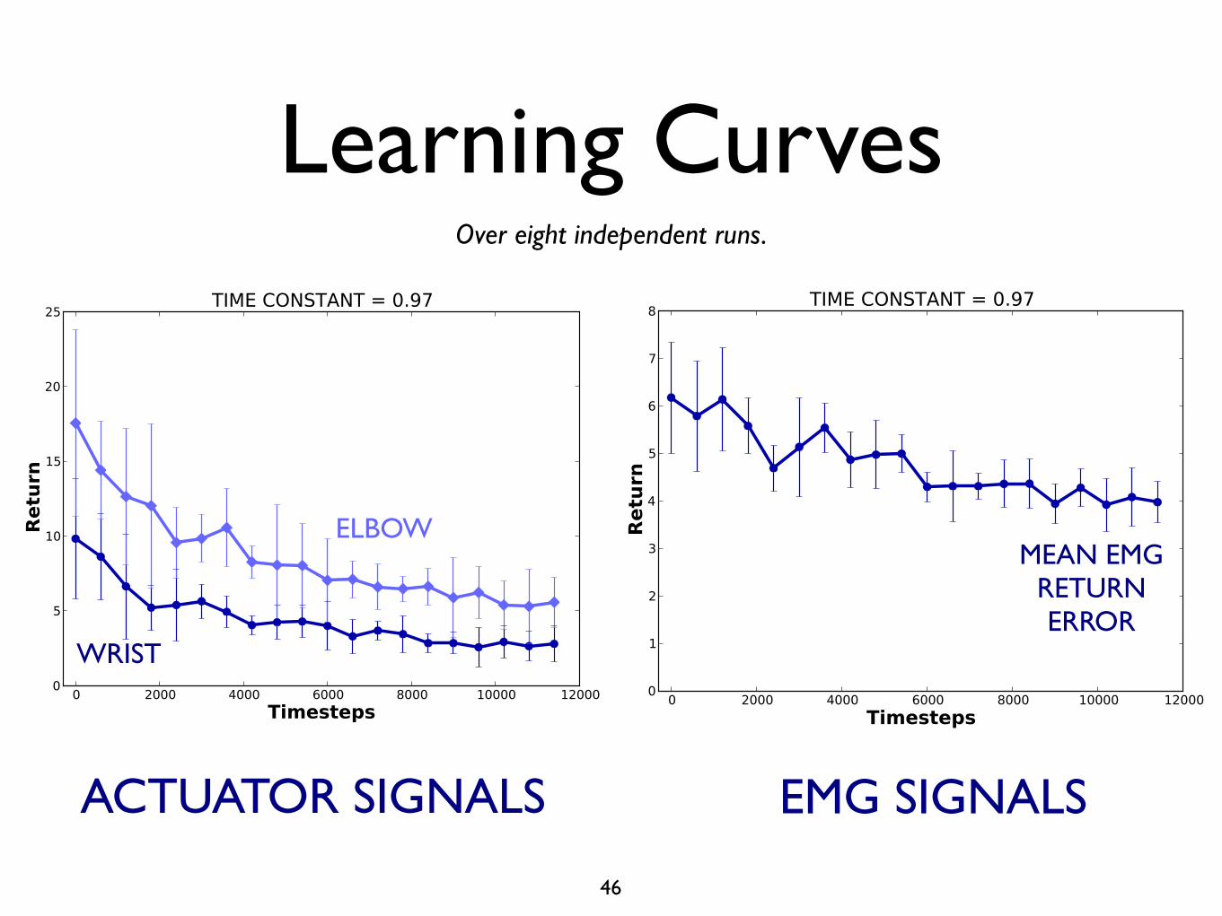
Learning CurvesOver eight independent runs.

ELBOW

WRIST

MEAN EMGRETURN ERROR

46

EMG SIGNALSACTUATOR SIGNALS

Clinical Experiments

• Approximately 20min of patient interaction with the MTT system (~60k timesteps).

• Recorded EMG signals, force signals, joint angle, joint speed, joint temp., joint load.

• Recording samples at 50Hz.

• GVF state = TileCoder(8,10) { EMG x 2, force, joint angle, joint speed}.

47

MEASUREDSIGNAL

CORRECTPRED.

T2 Pred

T1 Pred

T2 Pred

T1 Pred

Prediction ResultsAfter three iterations through the training data.

T1=0.97 T2=0.99

48

ANTICIPATIONRESULTS

VALIDATIONRESULTS

T2 Pred

T1 Pred

T2 Pred

T1 Pred

Results on Test DataAfter three iterations through the training data.

Testing data previously unseen by the system; no learning during testing evaluation.

49

ANTICIPATIONRESULTS

VALIDATIONRESULTS

MEASUREDSIGNAL

CORRECTPRED.

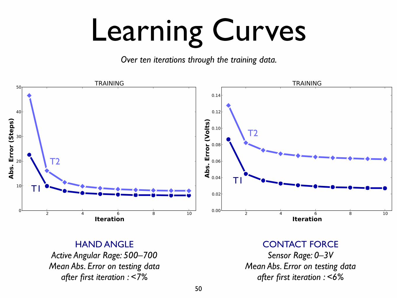
Learning Curves

HAND ANGLEActive Angular Rage: 500–700Mean Abs. Error on testing data

after first iteration : <7%

CONTACT FORCESensor Rage: 0–3V

Mean Abs. Error on testing dataafter first iteration : <6%

T2

T1

T2

T1

50

Over ten iterations through the training data.

Learning Curves

HAND ANGLEActive Angular Rage: 500–700Mean Abs. Error on testing data

after first iteration : <7%

CONTACT FORCESensor Rage: 0–3V

Mean Abs. Error on testing dataafter first iteration : <6%

T2

T1

T2

T1

51

Over ten iterations through the training data.

Summary• Real-time machine learning can help alleviate

barriers to assistive rehabilitation robotics.

• Recent work is on prediction and anticipation for improving the control of artificial limbs.

• Results: successful on-policy nexting for both patient data and able-bodied subject data.

• Big picture: artifical limbs that learn and improve through on-going user interaction.

52

• Dr. Richard S. Sutton, Dr. Thomas DegrisRLAI, Dept. Computing Science, University of Alberta

• Michael R. Dawson, Dr. Jacqueline S. Hebert, Dr. K. Ming ChanGlenrose Rehabilitation Hospital & University of Alberta

• Dr. Jason P. CareyDept. of Mechanical Engineering, University of Alberta

• Funders: Alberta Ingenuity Centre for Machine Learning (AICML), the Natural Sciences and Engineering Research Council (NSERC), Alberta Innovates – Technology Futures (AITF), and the Glenrose Rehabilitation Hospital Foundation.

53

Questions

... and thank you very much for your hospitality and attention.

[email protected]

http://www.ualberta.ca/~pilarski/

54

mailto:[email protected]

mailto:[email protected]



Real-time Machine Learning for Assistive Medical...

Documents

Transcript of Real-time Machine Learning for Assistive Medical...