REAL-TIME DSP LABORATORY6:The Fast Fourier Transform (FFT) and BlockConvolution FIR filtering on the C6713 DSK

Contents

1 Introduction 1

2 The Discrete Fourier Transform (DFT) 1

3 A Fast Fourier Transform (FFT) Algorithm 2

3.1 An 8-point Decimation-in-Time FFT algorithm . . . . . . . . . . . . . . . . . . . 34 Implementing An FFT Algorithm on the C6713 DSK 7

4.1 The Bit-Reversing Algorithm* . . . . . . . . . . . . . . . . . . . . . . . . . . . . 84.2 Implementing the Factored Butterfly* . . . . . . . . . . . . . . . . . . . . . . . . 9

5 FIR Filtering using an FFT Algorithm 15

5.1 Real-Time Block Processing on the C6713 DSK* . . . . . . . . . . . . . . . . . . 155.2 Linear Convolution using the DFT . . . . . . . . . . . . . . . . . . . . . . . . . . 175.3 Overlap and Add Block Convolution FIR Filtering* . . . . . . . . . . . . . . . . . 175.4 Implementing the Overlap and Add Algorithm using an FFT* . . . . . . . . . . . . 18

6 End Notes 20

6.1 Advanced Lab Topics . . . . . . . . . . . . . . . . . . . . . . . . . . . . . . . . . 20

1 Introduction

The discrete Fourier Transform (DFT) is the only Fourier transform that can be computedexactly on a digital computer, if by exact we ignore finite precession effects. The DFT, whenimplemented directly, requires many complex multiplications and additions. When an N -pointDFT is highly composite (i.e. N is a power of 2), the number of complex multiplicationsand additions may be reduced significantly by efficiently factoring the DFT. These factoredDFT algorithms are collectively known as fast Fourier Transform (FFT) algorithms. The FFTalgorithm was introduced to signal processing in 1965 in a paper published by J. W. Cooleyand J. W. Tukey [3]. However, the earliest known discovery of this factorization is credited toC.F. Gauss in 1805 [5], and in 1965 there actually existed some efficient codes that were nearlyequivalent to the FFT.

In this lab, you will study

• the DFT,• the in-place decimation-in-time FFT on the DSK using a C language program, and• FIR filter implementation using the FFT for fast convolution.

2 The Discrete Fourier Transform (DFT)

The discrete Fourier transform, or DFT, is a one-to-one mapping between an N -point complexdiscrete-time sequence {x[n], n = 0, 1, . . . N−1} and an N -point complex Fourier series sequence

1

{X[m],m = 0, 1, . . . N − 1}. The resulting Fourier transform pair is denoted {x[n], nto}N ←→{X[m], mωo

N }N , where

X[m] =

N−1∑

n=0

x[n]W−mnN (analysis) (1)

x[n] =1

N

N−1∑

m=0

X[m]WmnN (synthesis), (2)

where WN = ej2πN and Wmn

N are the N roots of unity on the unit circle in the complex plane.Here, the signal samples are spaced every nto seconds in times, and the FS coefficients, X[m],are spaced every mωo

N radians per second in frequency. When no confusion will result, we willuse the simpler notation {x[n]}N ←→ {X[m]}.

From Fourier analysis, we know that if a signal is discrete in one domain, then its Fouriertransform will be periodic. Since the DFT is discrete in both frequency and time, it is periodic inboth time and frequency. Consequently, both x[n] andX[m] areN -periodic (i.e. x[n] = x[n+rN ]and X[m] = X[m+ rN ] for all integers r.)

3 A Fast Fourier Transform (FFT) Algorithm

The direct computation of an N -point DFT requires N2 complex multiplications and N2 − Ncomplex additions [6]. In terms of real computing, this translates to 4N2 real multiplicationsand 2N2 + 2(N2 − N) = 4N2 − 2N real additions1 [6]. These arithmetic operations may bereduced significantly by using the following two properties about the roots of unity W k

N (wherek is an integer) [7]:

Symmetry property: Wk+N/2N = −W k

N (3)

Periodicity property: W k+NN = W k

N . (4)

When N is a power of two (i.e. N = 2ν , where ν = log2 N is an integer), a radix-2 FFT algorithmmay be used to efficiently compute a DFT. There are two ways of implementing a radix-2FFT, namely decimation-in-time and decimation-in-frequency. Since these two algorithms aretransposes of each other, only the decimation-in-time algorithm will be derived.

To begin this factorization, the DFT sum in eqn (1) is split into a sum of two N/2 length sums,one on the even indices of x[n] and one on the odd indices. This process is illustrated below [6,pg. 635–636]:

1The complex multiplication of two numbers z1 = x1+jy1 and z2 = x2+jy2 is z1z2 = (x1x2−y1y2)+j(x1y2+x2y1), which requires four real multiplications and two real additions. The addition of the two complex numbersz1 and z2 is z1 + z2 = (x1 + x2) + j(y1 + y2), which requires two real additions. Note that complex arithmeticrequires “two channel” variables that hold the real and imaginary parts of the complex number.

2

X[m] =

N2−1∑

n=0

x[2n]W−m(2n)N +

N2−1∑

n=0

x[2n+ 1]W−m(2n+1)N

=

N2−1∑

n=0

x[2n](W 2N )−mn +W−m

N

N2−1∑

n=0

x[2n + 1](W 2N )−mn (5)

=

N2−1∑

n=0

x[2n]W−mnN/2 +W−m

N

N2−1∑

n=0

x[2n+ 1]W−mnN/2 (6)

= G[m] +W−mN H[m],m = 0, 1, . . . , N − 1. (7)

Equation (6) uses the fact that W 2N = e(j

2πN

)2 = e(j 2π

N/2)= WN/2 to show how an N -point DFT

may be split into the sum of two N/2-point DFTs, namely G[m] andH[m] in eqn (7). Now, theseN/2 DFTs are periodic in m with period N/2 (i.e. G[m] = G[m+ rN

2 ] and H[m] = H[m+ rN2 ]

for all integers r). This process of grouping the even and odd indexed terms of x[n] into twoN/2 point DFTs is known as time decimation. As a result of this factorization, the number of

complex multiplications has been reduced from N2 to (N2 )2 + (N2 )

2 + N = N2

2 + N , where theextra N multiplications are for multiplying the coefficients H[m] by W−m

N ,m = 0, 1, . . . , N − 1.This factorization has reduced the number of complex multiplications roughly in half. Thisprocess may be repeated log2N times until there are N

2 2-point FFT factored butterflies perstage and log2N stages. The final factorization uses the symmetry property to reduce thenumber of multiplications required in half. The discussion in the following paragraph clarifiesthis point.

3.1 An 8-point Decimation-in-Time FFT algorithm

To begin factoring an 8-point DFT sum, we group the even and odd terms of the sequence{x[n]}8 and perform two 4-point DFTs as follows [6]:

X[m] =

8∑

n=0

x[n]W−mn8 (8)

=

3∑

n=0

x[2n]W−mn4 +W−m

8

3∑

n=0

x[2n + 1]W−mn4 (9)

= G[m] +W−m8 H[m], k = 0, 1, . . . , 7. (10)

Here, G[m] =3∑

n=0x[2n]W−mn

4 is the result of a 4-point DFT on the even indices of {x[n]}8, and

H[m] =3∑

n=0x[2n + 1]W−mn

4 is the result of a 4-point DFT on the odd indices of {x[n]}8. This

is called decimation-in-time. We may draw the signal flow graph for this once-factored DFT asshown in Figure 1.

3

X[0]

X[1]

X[2]

X[3]

X[4]

X[5]

X[6]

X[7]

08W

18W

28W

38W

48W

58W

68W

78W

4-point

DFT

4-point

DFT

G[0]

G[1]

G[2]

G[3]

H[0]

H[1]

H[2]

H[3]

x[0]

x[4]

x[6]

x[1]

x[3]

x[5]

x[7]

x[2]

Figure 1: Once factored 8-point DFT. Adapted from [6].

This process may be repeated one more time to yield

X[m] =

(1∑

n=0

x[4n]W−mn2 +W−m

4

1∑

n=0

x[4n + 2]W−mn2

)

+ W−m8

(1∑

n=0

x[4n+ 1]W−mn2 +W−m

4

1∑

n=0

x[4n + 3]W−mn2

), (11)

where the four summations are each 2-point sub-DFTs on indices separated by four. Each suminside the parenthesis is a 4-point sub-DFTs that amounts to a recombination of two 2-pointsub-DFTs (one on the even indices and one on the odd indices). The sum of the two 4-pointsub-DFTs is an 8-point sub-DFT that amounts to a recombination of the two 4-point sub-DFTs.Using the facts that W k

2 = W 4k8 and W k

4 = W 2k8 along with the fact that W 4k

8 is periodic in kwith period 2 and W 2k

8 is periodic in k with period 4 yields the final radix-2 FFT factorizationof an 8-point DFT2. This is shown in Figure 2.

!

2To further clarify this, note that in eqn (11) when n = 0 in each of the 2-point sums (i.e. sums involvingthe time samples x[0], x[1], x[2], and x[3]), W−mn

2= W 0

2 = 1, so these time samples are not scaled in the firststage. When n = 1 in each of the 2-point sums (i.e. sums involving the time samples x[4], x[5], x[6], and x[7]),W−mn

2= W−m

2, which is equal to W 0

2 when m is even and W−1

2when m is odd. Bearing in mind that W 0

2 = W 0

8

and W−1

2= W−4

8, use these facts to justify the first stage of Figure 2.

4

X[0]

X[1]

X[2]

X[3]

X[4]

X[5]

X[6]

X[7]

08W

18W

28W

38W

48W

58W

68W

78W

x[0]

x[4]

x[6]

x[1]

x[3]

x[5]

x[7]

x[2]

08W

28W

48W

68W

48W

68W

08W

28W

48W

48W

48W

48W

08W

08W

08W

08W

Figure 2: Final factorization of an 8-point DFT. Adapted from [6].

5

By inspecting Figure 2, there are 8 log2 8 = 24 complex multiplications (W−m8 factors). The

direct calculation of an 8-point DFT would require 82 = 64 complex multiplications. This FFTfactorization has reduced the number of complex multiplications by 40, which means that thisalgorithm will run at rate 64/24 = 2.67 times faster than a direct 8-point DFT computation.

When we implement the FFT algorithm shown in Figure 2, we will over-write the set of Nregisters from the previous stage. This is known as an in-place algorithm. Implementing anin-place algorithm will use the minimum number of memory locations, but it will not save theN input samples. Before we implement an in-place algorithm, we utilize a symmetry condition,which will further cut the number of complex multiplications in half. Notice that at each stage,a set of two nodes from one stage is used to compute the same two nodes in the next stage.Each of these mappings is of the form shown in Figure 3.

(l -1) - th

stage

l - th

stage

k

NW

−

k

N

Nk

NWW

−+− −=)2/(

Figure 3: The basic butterfly structure in a radix-2 decimation-in-time FFT algorithm. Adaptedfrom [6].

The structure in Figure 3 is referred to as a butterfly. For a radix-2 decimation-in-time FFTalgorithm, the butterfly structures have the same pattern. In particular, the value at the topnode in the l-th stage is the value at the top node from the (l − 1)-th stage plus the valueof the bottom node of the (l − 1)-th stage scaled by the complex value W−k

N . The value atthe bottom node in the l-th stage is the value at the top node from the (l − 1)-th stage plus

the bottom node scaled by W−(k+N/2)N . From the symmetry condition in eqn (3), we know that

W−(k+N/2)N = −W−k

N . Now, the value at the bottom node in the l-th stage may also be calculatedby taking the value at the top node from the (l − 1)-th stage and subtracting the value of thebottom node of the (l − 1)-th stage scaled by the complex value W−k

N . This observation leadsto the in-place butterfly structure shown in Figure 4.

(l -1) - th

stage

l - th

stage

k

NW

− -1

a

b

bWaak

N

−+=′

bWabk

N

−−=′

Figure 4: The in-place butterfly structure in a radix-2 decimation-in-time FFT algorithm.Adapted from [6].

When this butterfly structure is implemented in an in-place algorithm, the value in the bottomnode of the (l − 1)-th stage is first copied to a temporary variable which is scaled by a twiddlefactor. This happens before either node has been over-written. Then, the bottom node in

6

the l-th stage of the butterfly is computed and the value over-writes the bottom node. Afterthe bottom node in the l-th stage is calculated in-place, the value in the temporary variableis used to calculate the the value of the top node in the l-th stage, which over-writes the topnode. This extra memory requirement is unavoidable in an in-place implementation. However,in assembly code, this temporary variable would be stored in core register and not saved to amemory location. The final in-place decimation-in-time signal flow graph for an 8-point FFTalgorithm is shown in Figure 5. Notice that only 12 complex multiplications are required inthis 8-point FFT algorithm. Also, only the first N/2 roots of unity know are required for thisimplementation. These roots of unity W k

N for k = 0, 1, . . . , (N/2) − 1 are known as the twiddle

factors. In this FFT algorithm, the complex conjugates of the twiddle factors are needed. Apoint to be clarified later. In general, an N -point in-place decimation-in-time FFT algorithmwill require N

2 log2(N) complex multiplications and N log2(N) complex additions.

X[0]

X[1]

X[2]

X[3]

X[4]

X[5]

X[6]

X[7]

x[0]

x[4]

x[6]

x[1]

x[3]

x[5]

x[7]

x[2]

08W

28W

08W

28W

08W

28W

38W

18W

-1

-1

-1

-1

-1

-1

-1

-1

08W

08W

08W

08W

-1

-1

-1

-1

Figure 5: The in-place decimation-in-time signal flow graph for an 8-point FFT algorithm.Adapted from [6].

The trick in the decimation-in-time algorithm is to organize the N input samples in bit-reversed

order. By this, we mean that we represent the original indices as (log2 N)-bit binary numbersin chronological order, and then reverse the bits to create the bit-reversed order. In the caseN = 8, the 3-bit bit-reversed order observed in Figure 5 is illustrated in Table 1.

This re-arrangement can be seen in the arrangement of the inputs in the FFT flow graph inFigure 2.

4 Implementing An FFT Algorithm on the C6713 DSK

In this lab, we will create C code to implement an N -point FFT algorithm, where N is a powerof 2. To begin, let’s create the C code function FFT func(COMPLEX *X, COMPLEX *W) that willtake the N input samples, namely {x[n]}N , stored in the complex array X[], and use the N/2

7

n (dec) n (bin) bit-reversed (bin) bit-reversed (dec)

0 000 000 01 001 100 42 010 010 23 011 110 64 100 001 15 101 101 56 110 011 37 111 111 7

.

Table 1: Bit-reversing for an 8-point FFT algorithm.

twiddle factors in W[] to compute the N Fourier series coefficients, namely X[k], in-place. Thisalgorithm will over-write the same N registers at each stage of the algorithm. This process willbe broken up into two sections:

• Arrange the N inputs in bit-reverse order.• Compute the N/2 butterflies at each of the log2N stages.

4.1 The Bit-Reversing Algorithm*

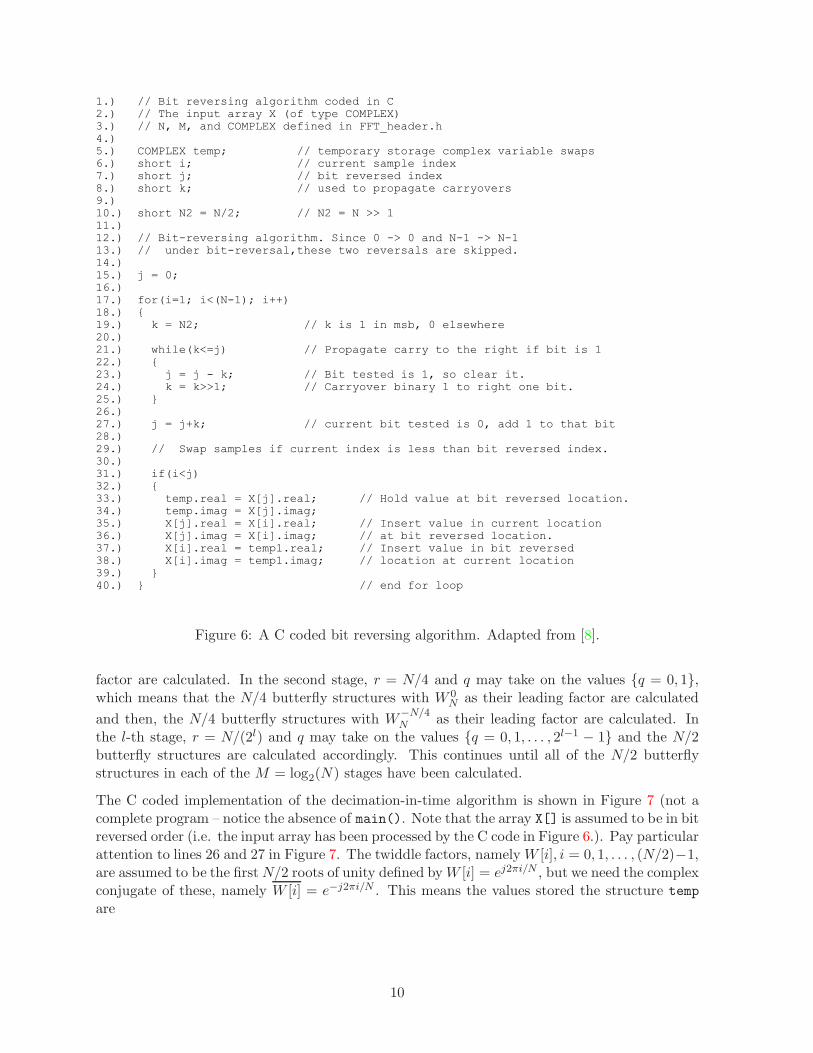
By comparing the binary values in Table 1, one can see that the bit-reversed order may becalculated by adding a binary one to the most significant bit and having the carryover bitspropagate to the right. To begin this process, start with binary zero and add a binary one tothe most significant bit (i.e. add N/2 in binary to zero). To calculate the next bit reversedindex, test the most significant bit to see if it is a binary zero or binary one. If the bit is binaryzero, add a binary one to it and move on to the next index. If this bit is a binary one, set it tobinary zero and try to add a binary one to the next least significant bit (carryover to the right).If this bit is a binary zero, add a binary one to it and move to the next index; otherwise, clearit and move to the next bit and repeat the process. This continues until a binary zero is foundor the last bit-reversed index has been calculated. Due to the way this is implemented, the lastindex will be calculated before an overflow to the right occurs.

To visualize this, we will work through a bit reversed sequence for M = 3 (N = 8 as in Table1). First, we observe that 000(bin) maps to 000(bin) and that 111(bin) maps to 111(bin), sothese indices are not calculated. The first bit-reversed index is N/2, which in our case is equalto 4. For intuition into the bit-reversing algorithm, we will represent the decimal number 4 asthe binary number 100(bin).

To calculate the next bit-reversed index, we try to add 100(bin) to our previous bit-reversedindex, 100(bin). Since the most significant bit in the previous bit-reversed index is a binary one,we clear it by subtracting 100(bin) from the number to get 100(bin) - 100(bin) = 000(bin) toclear the most significant bit. Then, we try to add 010(bin) to 000(bin), which is the result ofthe previous subtraction (clearing the most significant bit). Since the next least significant bitis a binary zero, our new bit-reversed index becomes 000(bin) + 010(bin) = 010(bin).

8

To calculate the next bit-reversed index, we again try to add 100(bin) to the previous bit-reversed index, 010(bin). Since the most significant bit in 010(bin) is a binary zero, our newbit-reversed index becomes 010(bin) + 100(bin) = 110(bin).

To calculate the next bit-reversed index, we again try to add 100(bin) to our previous bit-reversedindex, 110(bin). Since the most significant bit is a binary one, we clear it by subtracting 100(bin)to get 110(bin) - 100(bin) = 010(bin). Then, we try to add 010(bin) to 010(bin). Since thenext least significant bit in 010(bin) is a binary one, we clear it by subtracting 010(bin) to get010(bin) - 010(bin) = 000(bin). Then, we try to add 001(bin) to 000(bin). Since the next leastsignificant is a binary zero, our new bit-reversed index becomes 000(bin) + 001(bin) = 001(bin).

This process continues until all N bit-reversed indices have been calculated. In practice, we takeadvantage of the fact that the first and last indices map to themselves, so we only calculate theN − 2 indices in between.

Examine the code for the bit-reversing algorithm and associated data swaps listed in Figure6. Note that this is not a complete program but just a fragment of code. Observe that thebit-reversal mapping is a one-to-one mapping, so we can swap the value at the current indexwith the value at the bit-reversed index. This can be done in-place using a temporary storagevariable, which is illustrated in lines 34 and 35 in Figure 6. Also, the swapping of values betweenthe original and bit reversed indices only needs to occur once. To account for this, we test thecurrent index with the bit-reversed index and only swap if the current index is less than thebit-reversed index. Then, when the current index is greater than the bit-reversed index, weknow that the values have already been swapped. This is coded in line 32 of Figure 6, where iis the current index and j is the bit-reversed index of i.

Assignment

1. Work through the description of the 8-point bit-reversing algorithm given on the pre-vious page using decimal numbers instead of binary numbers. Then, briefly explainhow the C code in lines 17-27 of Figure 6 implement the bit-reversing algorithm. NB:If k=01100bin (which has decimal equivalent k = 12dec), then the C command k>>1

returns the binary number 00110bin (which has decimal equivalent 6dec) meaning itshifts all of the bits one to the right (and discards the least significant bit). This is theequivalent of dividing the decimal number k = 12dec by 2 (i.e. 12/2 = 6).

4.2 Implementing the Factored Butterfly*

Once the input samples have been put into bit reversed order, we can implement the in-placedecimation-in-time signal flow graph shown in Figure 5. This signal flow graph is implementedby grouping the butterfly structures at each stage according to their leading twiddle factors.First, all of the butterfly structures that have W 0

N as their leading factor are calculated. Then,the butterfly structures with W−r

N as their leading factor are calculated. Then, the butterflystructures with W−2r

N as their leading factor are calculated, and so on until the N/2 butterfly

structures with the W−qrN as their leading factor have been calculated at a given stage. Here,

qr < N/2, and q and r are non-negative integers. In the first stage, r = N/2 and q may takeon the value {q = 0}, which means that the N/2 butterfly structures with W 0

N as their leading

9

1.) // Bit reversing algorithm coded in C2.) // The input array X (of type COMPLEX) 3.) // N, M, and COMPLEX defined in FFT_header.h4.)5.) COMPLEX temp; // temporary storage complex variable swaps6.) short i; // current sample index7.) short j; // bit reversed index8.) short k; // used to propagate carryovers9.)10.) short N2 = N/2; // N2 = N >> 111.)12.) // Bit-reversing algorithm. Since 0 -> 0 and N-1 -> N-113.) // under bit-reversal,these two reversals are skipped.14.)15.) j = 0;16.)17.) for(i=1; i<(N-1); i++)18.) {19.) k = N2; // k is 1 in msb, 0 elsewhere20.)21.) while(k<=j) // Propagate carry to the right if bit is 122.) {23.) j = j - k; // Bit tested is 1, so clear it.24.) k = k>>1; // Carryover binary 1 to right one bit.25.) }26.)27.) j = j+k; // current bit tested is 0, add 1 to that bit28.)29.) // Swap samples if current index is less than bit reversed index.30.)31.) if(i<j)32.) {33.) temp.real = X[j].real; // Hold value at bit reversed location.34.) temp.imag = X[j].imag;35.) X[j].real = X[i].real; // Insert value in current location36.) X[j].imag = X[i].imag; // at bit reversed location.37.) X[i].real = temp1.real; // Insert value in bit reversed38.) X[i].imag = temp1.imag; // location at current location39.) }40.) } // end for loop

Figure 6: A C coded bit reversing algorithm. Adapted from [8].

factor are calculated. In the second stage, r = N/4 and q may take on the values {q = 0, 1},which means that the N/4 butterfly structures with W 0

N as their leading factor are calculated

and then, the N/4 butterfly structures with W−N/4N as their leading factor are calculated. In

the l-th stage, r = N/(2l) and q may take on the values {q = 0, 1, . . . , 2l−1 − 1} and the N/2butterfly structures are calculated accordingly. This continues until all of the N/2 butterflystructures in each of the M = log2(N) stages have been calculated.

The C coded implementation of the decimation-in-time algorithm is shown in Figure 7 (not acomplete program – notice the absence of main(). Note that the array X[] is assumed to be in bitreversed order (i.e. the input array has been processed by the C code in Figure 6.). Pay particularattention to lines 26 and 27 in Figure 7. The twiddle factors, namely W [i], i = 0, 1, . . . , (N/2)−1,are assumed to be the firstN/2 roots of unity defined byW [i] = ej2πi/N , but we need the complexconjugate of these, namely W [i] = e−j2πi/N . This means the values stored the structure temp

are

10

Re{temp} = Re{X[i lower]}Re{W [i]} − Im{X[i lower]}Im{W [i]}

= Re{X[i lower]}Re{W [i]}+ Im{X[i lower]}Im{W [i]}

Im{temp} = Im{X[i lower]}Re{W [i]}+Re{X[i lower]}Im{W [i]}

= Im{X[i lower]}Re{W [i]} − Re{X[i lower]}Im{W [i]},

where i lower is the the index of the lower butterfly node for a given stage and twiddle factor.The variable temp is used to store the value of the lower node scaled by the conjugate of thetwiddle factor. This is required so the in-place algorithm can calculate and overwrite the valuesin the lower node at current stage in lines 29 and 30 and still have the value of the scaled lowernode at the current stage to calculate and overwrite the top node in lines 32 and 33. This is aprogramming concern that comes up often when two or more registers are used for accumulatingor in-place processing. This problem is easily solved by using temporary registers.

For sake of clarity, note that the variables step and stage code the variables r and l from theprevious discussion, respectively. Also, at each stage, q takes on the values {0, 1, . . ., numBF-1}.

For the final C coded decimation-in-time FFT algorithm, the code in Figure 7 is integratedwith the code from Figure 6, along with the header file FFT header.h, to create the C callablefunction FFT func.c that we will use to implement our FFT algorithm. In the case that N = 8,the header file FFT header.h is listed in Figure 8. This header files defines the structure COMPLEX(see Lab 2) and the order of the FFT to be implemented. This header file may be created usingthe homebrew MATLAB function FFT header gen.m, which is available on the class webpage.Download this file and use it to re-create the file listed in Figure 8.

The C program that we will use to test our FFT function is shown in Figure 9, which alsoincludes FFT header.h. Together, the C code in Figures 6, 7, 8, and 9 have been groupedtogether into the project FFT test.pjt that is available on the class webpage. You are expectedto create a header file like the one listed in Figure 8 using the MATLAB function provided.Download this project file and accompanying files, FFT test.c and FFT func.c, and create theheader file in MATLAB. Open the project in CCS, and implement it on the DSK to verify thatthe FFT algorithm is working correctly.

NB: the program FFT test.c does not terminate in an infinite loop as do programs which usethe codec – it runs to completion and then stops at an exit location. In order to re-run it,you can either reload the program or click on Debug → Restart followed by Debug →Run

11

1.) // N, M, COMPLEX defined in FFT_header.h, N2=N/2 (pre-defined) 2.) // COMPLEX W[N2] // twiddle factors, passed to FFT_func.c 3.) COMPLEX temp; // temporary storage complex variable 4.) short i,j,k; // loop indices 5.) short i_lower; // Index of lower point in butterfly 6.) short step; 7.) short stage; // FFT stage 8.) short DFTpts; // # of points in sub DFT and offset to next DFT 9.) short numBF; // # of butterflies in one DFT, offset to lower node 10.)11.) // Assume X[] is in reverse-bit order and do the M=log2(N) stages of butterflies 12.) step = N2; // step = N/2, N/4, N/8, ... 1 13.) for(stage=1; stage <= M; stage++) 14.) { 15.) DFTpts = 1 << stage; // DFTpts = 2^stage = points in sub DFT 16.) numBF = DFTpts/2; // number of butterflies in sub-DFT 17.) k = 0; // initial twiddle factor index 18.)19.) // Do butterflies for current stage 20.) for(j=0; j<numBF; j++) // do the numBF butterflies per sub DFT 21.) {22.) // Compute butterflies that use same twiddle factor, W[k] 23.) for(i=j; i<N; i += DFTpts) 24.) { 25.) i_lower = i + numBF; // index of lower point in butterfly 26.) temp.real = X[i_lower].real*W[k].real + X[i_lower].imag*W[k].imag; 27.) temp.imag = X[i_lower].imag*W[k].real - X[i_lower].real*W[k].imag; 28.)29.) X[i_lower].real = X[i].real - temp.real; 30.) X[i_lower].imag = X[i].imag - temp.imag; 31.)32.) X[i].real = X[i].real + temp.real; 33.) X[i].imag = X[i].imag + temp.imag; 34.) } 35.) k += step; // increment twiddle index 36.) } 37.) step = step/2; // calculate step for next stage 38.) }

Figure 7: A C coded decimation-in-time algorithm. Adapted from [8].

Assignment

2. Using the DSK and the project FFT test.pjt, located on the class webpage, calculatethe FS coefficients for {x[n] = cos(3π8 n), n = 0, 1, . . . , 15}. What are the values of N,M, and N2? Calculate the 16 discrete Fourier series coefficients by hand using eqn (1)to verify that the C coded FFT function is working properly. If the sample rate ofthe system were fo = 8kHz, then what frequencies would the non-zero FS coefficientscorrespond to? If the sequence x[n] were aliased every 16 samples (i.e. x[n] = x[n+16r]for every integer r) and sent to the on-board codec, what would the output be?

3. Create a function that implements an in-place inverse FFT. Label this functionIFFT func.c. This function should have two complex arrays passed to it, namelyX[] and W[], where X[] will contain the array of elements that the IFFT algorithmwill operate on in-place, and W[] will contain the N/2 twiddle factors. These twiddlefactors should be the same as those used in FFT func.c. Explain what changes needto be made to convert an FFT algorithm to an IFFT algorithm. (HINT: Compareequations (1) and (2).) Use the output of the FFT evaluated in question 3 as yourinput to your IFFT function. What is the output? (HINT: If your IFFT algorithmis working correctly, you will find that the cascade of the FFT and the IFFT is theidentity operator. Thus the output of cascade is the input.)

12

// FFT header . h// This f i l e must be inc luded in FFT func . c// and by the program that c a l l s FFT func . c

#de f i n e N 8 // N−point FFT#de f i n e M 3 // M=log2 (N)#de f i n e N2 4 // N/2 (number o f tw idd le f a c t o r s )#de f i n e PI 3.14159265358979 // f ix ed−point approx . to p i

typedef s t r u c t { f l o a t r ea l , imag ;} COMPLEX; // s t r u c tu r e COMPLEX

Figure 8: A listing of FFT header.h for N = 8

13

// FFT test . c// Used to t e s t FFT func . c// N−po int FFT, where N i s de f ined in FFT header . h/∗1 ∗/ #inc lude <math . h>/∗2 ∗/ #inc lude <s t d i o . h>/∗3 ∗/ #inc lude ”FFT header . h” // d e f i n e s COMPLEX s t r u c tu r e/∗4 ∗/ // and FFT order/∗5 ∗/ void FFT func (COMPLEX ∗X, COMPLEX ∗W) ; // FFT func t i on prototype/∗6 ∗//∗7 ∗/ COMPLEX X[N] ; // Dec la re input ar ray/∗8 ∗/ COMPLEXW[N2 ] ; // Used to hold the N/2 twiddle f a c t o r s/∗9 ∗//∗10∗/ i n t main ( )/∗11∗/ {/∗12∗/ sho r t i ; // loop index/∗13∗//∗14∗/ // Ca l cu la t e twiddle f a c t o r s/∗15∗/ f o r ( i =0; i<N2 ; i++)/∗16∗/ {/∗17∗/ W[ i ] . r e a l = cos ( 2 . 0 ∗PI∗ i /N) ;/∗18∗/ W[ i ] . imag = s i n ( 2 . 0 ∗PI∗ i /N) ;/∗19∗/ }/∗20∗//∗21∗/ // I n i t i a l i z e input ar ray/∗22∗/ f o r ( i =0; i<N; i++)/∗23∗/ {/∗24∗/ X[ i ] . r e a l = cos ( ( f l o a t ) 2 .0∗PI∗3∗ i /N) ;/∗25∗/ X[ i ] . imag = 0 . 0 ;/∗26∗/ }/∗27∗//∗28∗/ FFT func (X,W) ; // perform in−p la ce FFT/∗29∗//∗30∗/ // Display r e s u l t s on s c r e en/∗31∗/ f o r ( i =0; i<N; i++)/∗32∗/ p r i n t f (”X[%d ] = \ t%10.5 f + j %3.5 f \n” , i , (X[ i ] ) . r ea l , (X[ i ] ) . imag ) ;/∗33∗/ return 0 ;/∗34∗/ }

Figure 9: A C coded program that tests our FFT algorithm. Adapted from [8].

14

5 FIR Filtering using an FFT Algorithm

5.1 Real-Time Block Processing on the C6713 DSK*

Now that we have working FFT and IFFT algorithms, we need to incorporate them into areal-time system. In this section, we will process blocks or vectors of data sequentially in timeinstead of calculating scalar outputs sequentially in time. To begin, let’s build a template forprocessing blocks of data on the C6713 DSK. We are going to implement the equivalent of thestraight wire program from Lab 2, but we will use it to test our FFT and IFFT algorithms.

N-point

FFT

N-point

IFFT

][ˆ nx][nx

N N

ADC DAC)(tx )(ˆ tx

Figure 10: Straight Wire using Coded FFT and IFFT Algorithms.

Consider the system in Figure 10. The sequence x̂[n] ≈ x[n], with discrepancies resulting fromfinite precision processing. However, these effects will be minimal due to the floating-pointalgorithm used. The trade-off is that the floating-point algorithm will take more clock cycles tocompute than a fixed-point algorithm would, but the finite precision effects will not need to bemanaged. A C code implementation of Figure 10 is given in Figure 11. Note that the functionsFFT func.c, IFFT func.c, and appropriate header files must be included with the project.

The idea in IO stream.c is that samples are read from the on-board codec, converted to floating-point numbers, and stored in the floating-point array io buffer (input - output buffer). Oncethis buffer is full, the samples are copied to a complex array structure labelled process, andpreviously processed data is copied to the array io buffer. While this is taking place, theimaginary part of the process array is set to zero. This is done since the samples being read inare assumed to be purely real. This may seem redundant since the output in the process arrayis assumed to be real, but due to finite precision effects, the imaginary part of the output maynot be exactly equal to zero. Next, the FFT algorithm is applied to the data in the process

array in the main() function, while an interrupt is used to output previously processed samplesand read in new samples. Now, as a sample is outputted from a memory location in the arrayio buffer, a new sample is read into the same memory and a global counter (ctr in Figure 11)is used to point to the next memory location in io buffer. This continues until io buffer isfull, at which point the procedure is repeated.

The DSP algorithm waits for the io buffer to fill in line 28. Once the buffer is full, the variableflag is set to true in line 16 (located in the interrupt) and the algorithm, upon return fromthe interrupt, proceeds to line 30, where it resets the flag variable to false. Then, in lines31 through 37, the data in io buffer is transferred to the real channel of the process array,the imaginary part of the process array is zeroed, and previously processed data is moved tothe io buffer. These data transfers will take place between the time the last sample of theprevious block was read in from the codec and the time the first sample of the next block is sentto the codec. Therefore, the DSP chip will have roughly Nto seconds to process the rest of thealgorithm, where N is the length of the block being processed and to is the sample rate of thesystem.

15

/∗1 ∗/ // io s t r eam . c − i n c lude header f i l e s , f unct i on prototypes , and W[N2 ]/∗2 ∗/ COMPLEX proces s [N ] ;/∗3 ∗/ f l o a t tmp ;/∗4 ∗/ f l o a t i o b u f f e r [N ] ;/∗5 ∗/ shor t c t r =0;/∗6 ∗/ shor t f l a g =0;/∗7 ∗//∗8 ∗/ in t e r r up t void c i n t 11 ( ) // i n t e r r up t s e r v i c e r ou t in e/∗9 ∗/ {/∗10∗/ output sample ( ( shor t ) i o b u f f e r [ c t r ] ) ;/∗11∗/ i o b u f f e r [ c t r++]=( f l o a t ) input sample ( ) ;/∗12∗//∗13∗/ i f ( c t r >= N)/∗14∗/ {/∗15∗/ c t r =0;/∗16∗/ f l a g = 1 ;/∗17∗/ }/∗18∗/ return ; // return from in t e r r up t/∗19∗/ }/∗20∗//∗21∗/ void main ( )/∗22∗/ {/∗23∗/ shor t i ; // l o c a l counter/∗24∗//∗25∗/ // Ca l cu la t e twidd le f a c t o r s f o r ( I )FFT/∗26∗//∗27∗/ comm intr ( ) ;/∗28∗/ whi le (1 )/∗29∗/ {/∗30∗/ whi le ( f l a g ==0);/∗31∗//∗32∗/ // Once the bu f f e r i s f u l l , implement DSP algor i thm here/∗33∗/ f l a g = 0 ;/∗34∗//∗35∗/ f o r ( i =0; i<N; i++)/∗36∗/ {/∗37∗/ tmp = proce s s [ i ] . r e a l ;/∗38∗/ p roce s s [ i ] . r e a l = i o b u f f e r [ i ] ;/∗39∗/ p roce s s [ i ] . imag = 0 . 0 ;/∗40∗/ i o b u f f e r [ i ] = tmp ;/∗41∗/ }/∗42∗//∗43∗/ FFT func ( proces s , W) ; // perform in−p lace FFT/∗44∗/ IFFT func ( proces s , W) ; // perform in−p lace FFT/∗45∗/ }/∗46∗/ }

Figure 11: Stripped Down version of IO stream.c.

16

Assignment

4. Download the project IO stream.pjt, IO stream.c, and FFT header.h from the classwebpage. Incorporate your FFT and IFFT functions into this project and build andrun the project on the DSK. Verify that the program is implementing a straight wire.Notice that this FFT header file is designed for a 128-point FFT. This means that we areprocessing data in blocks of 128 samples. Now, once the buffer has filled and the datahas been swapped between the io buffer array and the process array, the algorithmhas about Nt0 = 128 ∗ .125ms (about 16ms) to execute the rest of the algorithm. Inreality, this algorithm will finish after only a sample or two has been read in from thecodec (about .25ms), so the DSK will be idle (ignoring the input and output of datavia the codec) for about 15.75ms for every block of data that is processed. This extratime will allow us to use the FFT (and IFFT) to implement block convolution, whichwe will discuss next. This project will serve as a template for doing block processing inreal-time.

5.2 Linear Convolution using the DFT

A property that holds for all Fourier transforms is that multiplication in one domain transformsto convolution in the other. Since the DFT is periodic in both domains, the convolution willbe cyclic in both domains. In this section, we wish to do linear convolution of two finite lengthsequences in the time domain by first calculating their respective DFTs, multiplying the DFTsterm-by-term3, and then taking the inverse DFT of the product to get the convolved timesequence. However, if we apply this process to the finite length sequences only, we will geta result that is the circular convolution and not the linear convolution of the two sequences.To get linear convolution from the DFT, we note that the convolution in time of two finitelength sequences, say x1[n] of length L and x2[n] of length Q, results in y[n] = (x1 ∗ x2)[n],which will be of length L + Q − 1. Using this fact, we can zero-pad the time sequences, sothey are both of length L + Q − 1. To do this, we define x̃1[n] = x1[n] for n = 0, 1, . . . , L − 1and 0 for n = L,L + 1, . . . , L + Q − 1, and x̃2[n] = x2[n] for n = 0, 1, . . . , Q − 1 and 0 forn = L,L + 1, . . . , L + Q − 1. Then, we can take the DFTs of x̃1 and x̃2, multiply the DFTsterm-by-term, and inverse DFT the product to get the desired linear convolution (x1 ∗ x2)[n].

5.3 Overlap and Add Block Convolution FIR Filtering*

In the previous programming example, IO stream.c, the output block size was the same as theinput block size, so there was no overlap between the blocks. However, when block convolution isimplemented, blocks of L samples will be read in from the codec and output blocks of N +Q−1samples will be produced, which will overlap by Q − 1 samples. This leaves two options fordealing with the overlap. Either, read in blocks of L samples, overlap the input blocks (i.e.make the last Q − 1 samples of a given input block the first Q − 1 samples of the next inputblock), convolve the input blocks with the filter response using an FFT method, and save thelast L samples, or read in blocks of L samples, convolve the input blocks with the filter responseusing an FFT method, and add the last Q− 1 samples (term-by-term) from the processed data

3It is assumed apriori that the two sequences are of the same length.

17

of a given block to the first Q − 1 samples of processed data in the next block. These twoalgorithms are known as the Overlap and Save and Overlap and Add methods, respectively [6].In this section, we will develop the overlap and add algorithm, which you will ultimately codein C. To visualize this algorithm, consider the sequence x[n] in the top panel of Figure 12.

x1[n]=x[n], n=0,1,2,3,4,5 L=6

x2[n]=x[n+L], n=0,1,2,3,4,5 L=6

x3[n]=x[n+2L], n=0,1,2,3,4,5 L=6

Figure 12: Splitting the input stream into blocks of length L = 6.

This input stream, x[n], is split into blocks of length L = 6 (shown in the bottom three panels ofFigure 12). Let the FIR filter h[n] be the 1kHz notch filter from lab 4 with duration 3 samples(i.e. Q = 3). Now, if each of the sequences x1[n], x2[n], and x3[n] is convolved with h[n], thenthe results will be of length N = 8, which are shown in the top three panels of Figure 13. Theoutput is then formed by summing these sequences vertically (term-by-term) to generate theoutput y[n].

Assignment

5. Consider the output y[n] in Figure 13 when n = 6, 7, 8, and 9. Show that the summa-tion of the overlap from the blocks (h ∗ x1)[n] and (h ∗ x2)[n] gives the desired resulty[n] = h[0]x[n] + h[1]x[n − 1] + h[2]x[n − 2]. (HINT: Use the linear shift-invariance ofconvolution.)

5.4 Implementing the Overlap and Add Algorithm using an FFT*

Located on the class webpage is a homebrew MATLAB function, Overlap Add header gen.m

that will create the header files you will need to implement an overlap and add algorithm. Thisfunction will create the header file FFT header.h and coeffs.h, where FFT header.h is thestandard FFT header file that we have been using. The new file, coeffs.h, must be included inthe C source code containing the main() function. This file will contain the filter coefficients,stored in the floating-point array h[], define the number of inputs to read in, L, and definethe number of samples to overlap, P. In the previous discussion, L was the number of samplesto read in, Q was the filter duration, and Q − 1 was the number of samples to overlap. Now,

18

(h*x1)[n]

(h*x2)[n]

(h*x3)[n]

y[n] = (h*x1)[n] + (h*x

2)[n] + (h*x

3)[n]

Figure 13: Convolved input blocks and final output y[n].

L remains the same, the number of samples to overlap is P = Q − 1, and the FFT order isN = L+P 4. Note that the function Overlap Add header gen.m can generate this informationfrom the filter coefficients h and the FFT order N, which are the two variables that must bepassed to the function. Download this function from the class webpage and use help and type

to see how this works.

For the overlap and add algorithm, you will need the following global variables:

• a complex structure of length N to hold the DFT of the filter response,• a complex structure of length of length N to use as a process buffer,• a floating-point array (IO buffer) of length L to interface the codec,• a floating-point array of length L to hold the samples to overlap from the previous block

of processed data; this array will also be used to store the final processed block of datathat will be copied to the IO buffer,

• temporary variable(s) for the complex multiplication of the filter FS coefficients with theDFT of the zero-padded input sequence, and

• other miscellaneous variables needed to implement any real-time block processing algo-rithm.

Once you have your variables in order, you must initialize some of the variables. Before thecodec is initialized, initialize the following:

• the twiddle factors, and• the discrete FS coefficients of the zero-padded filter impulse response.

After these initializations are made, initialize the codec, and code the overlap and add algorithmas follows (in the order given):

4Note that P is the filter order as it was defined in Lab 4, except the letter to denote this has been changedfrom N to P . This is done to avoid a conflict of variables with the FFT order N .

19

• copy the IO buffer into the first L memory locations in the process array and copy thepreviously processed data into the IO buffer,

• copy the last P samples from the process array into the overlap array and zero the lastL− P samples of the overlap array,

• zero the imaginary part of the process array and perform an in-place FFT on the array,• multiply the process array with the DFT of the zero-padded filter coefficients,• IFFT the process array,• add the first L samples of the process array to the overlap array, which will serve as the

output for the next block of data.

Assignment

6. Create a project that implements the overlap and add algorithm given above. Includea copy of the C source code that you used to achieve this. Briefly explain how yourprogram works. What is the filter latency? Numerically, compare the computationsrequired to implement this algorithm with the direct convolution of Lab 4.

6 End Notes

In this lab, we have explored the FFT algorithm and one of its applications to real-time systems.Other applications include spectrum analysis and orthogonal frequency division multiplexing(OFDM) for modulation and demodulation, which we will explore in more depth in later labs.

6.1 Advanced Lab Topics

• Implement a decimation in frequency FFT algorithms. Refer to [6].• Implement a radix-4 (or higher order radix) FFT algorithm.• Implement the DFT using recursive linear filter methods like the Goertzel algorithm and

the Chirp Z-transform algorithm. Refer to [6].• Implement an overlap and save block convolution FIR filter.

References

[1] Rulph Chassaing. DSP Applications Using C and the TMS320C6x DSK. Wiley, New York,2002.

[2] Colorado State University, Fort Collins, CO. Signals and Systems Laboratory 11: The FFT

and its Applications, 2001.

[3] J. W. Cooley and J. W. Tukey. An algorithm for the machine calculation of complex fourierseries. Mathematics of Computation, 19:297–301, 1965.

[4] Simon Haykin and Barry Van Veen. Signals and Systems. Wiley, New York, 1999.

20

[5] M.T. Heideman, D.H. Johnson, and C.S. Burrus. Gauss and the history of the fast fouriertransform. IEEE Transactions on Acoustics, Speech, and Signal Processing, 1:14–21, October1984.

[6] Alan V. Oppenheim and Ronald W. Schafer. Discrete-Time Signal Processing. PrenticeHall, Uper Saddle River, NJ, 1989.

[7] John G. Proakis and Dimitris G. Manolakis. Digital Signal Processing: Principles, Algo-

rithms, and Applications. Prentice Hall, Uper Saddle River, NJ, 1996.

[8] Steven A. Tretter. Communication Design Using DSP Algorithms: With Laboratory Exper-

iments for the TMS320C6701 and TMS320C6711. Kluwer Academic/Plenum Publishers,New York, 2003.

21