Real-time distributed video transcoding on a … · Real-time Distributed Video Transcoding on a...
113
Real-time Distributed Video Transcoding on a Heterogeneous Computing Platform Zhi Hao Chang Faculty of Engineering, Computing, and Science (FECS) Swinburne University of Technology Sarawak Campus, Malaysia Submitted for the degree of Master of Engineering 2017
Transcript of Real-time distributed video transcoding on a … · Real-time Distributed Video Transcoding on a...
Real-time Distributed Video Transcoding
on a Heterogeneous Computing Platform
Zhi Hao Chang
Faculty of Engineering, Computing, and Science (FECS)
Swinburne University of Technology
Sarawak Campus, Malaysia
Submitted for the degree of Master of Engineering
2017

Dedicated to ...
my beloved family
i
Abstract
The requirements for real-time video transcoding systems have been significantly in-
creased due to the easy and widely available access to high resolution video streams
and large-scale applications in recent years. These requirements basically comprise
processing video in-messages, resilient to missing & out-of-order frames, capability of
storing, accessing & modifying state information grouped along live streaming videos,
capability to distribute transcoding instances across multiple machines, deliver low la-
tency response times for high volume video transcoding applications and etc. In this
thesis, a real-time distributed video transcoding system working in a heterogeneous
environment has been proposed to tackle the high requirements of such applications.
It allows multiple computers on the same network to execute the same transcoding
task together. As such, the system can then process more video streams in real time.
The proposed approach emphasizes throughput of video data aggregation which in-
volves the continuous input video stream and outcomes of transcoded video streams
that are accessible on-the-fly in contrast to the batch-oriented approach such as the
MapReduce framework, where output latencies can be significant. Data transmission
in terms of micro batches of GOP is selected as the granularity level of data in the
proposed system. This is to ensure maximum system throughput obtained by incorpo-
rating the trade-off between computation and communication overheads. Besides that,
an offline resource-aware task allocation scheme is proposed and has exhibited a fair
amount of tasks allocated among heterogeneous computers.
The performance of the proposed system can be further optimized by using a more in-
telligent scheduler and dynamic task allocation strategies for an optimal fair workload
distribution among heterogeneous computing systems.
ii
Acknowledgments
This master research study is made possible through the financial support from Sarawak
Information System Sdn. Bhd. as part of a bigger project: "A High Performance Net-
work Video Recorder and Video Management Systems". Swinburne University of Tech-
nology has also kindly provided research studentship funding for my postgraduate
study, for which I am deeply indebted.
First, my sincere gratitude goes to my main supervisor, Professor M. L. Dennis Wong
for the continuous support, his individual insights, patience, immense knowledge,
kindness and the motivation he provided for the accomplishment of this dissertation.
His guidance helped me always at the time of doing research, in keeping my research
focused and on track throughout my Master degree. It was an honour for me to work
under his supervision.
In addition, I also want to thank my co-supervisor Dr. Ming Ming Wong, who reminded
me to look for research topics when the project first kick started, not just only focus on
project milestones and deliverables. My sincere thanks also go to Associate Professor
Wallace Shung Hui Wong, David Lai Soon Yeo, Mark Tze Liang Sung, Lih Lin Ng,
who provided me an opportunity to participate in a collaborated project by Sarawak
Information Systems (SAINS) Sdn. Bhd. and Swinburne Sarawak (SUTS).
My thanks to my fellow friends, Dr. Nguan Soon Chong, Dr. Wei Jing Wong, Dr. Lin
Shen Liew, Bih Fei Jong, Wen Long Jing, Jia Jun Tay, Ivan Ling and Tien Boh Luk, for
being the most stimulating discussion group that I have had in the past two years. My
gratitude goes to Bih Fei Jong, Dr. Nguan Soon Chong, Dr. Wei Jing Wong, Ivan Ling,
and Derick Tan who were my project partners and who contributed their time and
effort throughout the project milestones.
Last but not least, I would like to thank my parents, my brother and sister for encour-
aging me to pursue my Master degree and in supporting me spiritually throughout all
these years.
iii

Declaration
I declare that this thesis contains no material that has been accepted for the award of
any other degree or diploma and to the best of my knowledge contains no material
previously published or written by another person except where due reference is made
in the text of this thesis.
CHANG ZHI HAO
iv
Publications Arising from this
Thesis
[1] Z. H. Chang, B. F. Jong, W. J. Wong, M. L. D. Wong, “Distributed Video Transcod-
ing on a Heterogeneous Computing Platform”, IEEE APCCAS 2016, Jeju Island, Korea,
October, 2016. pp. 444-447
[2] B. F . Jong, Z. H. Chang, W. J. Wong, M. L. D. Wong, and S. K. D. Tang, “A WebRTC
based ONVIF Supported Network Video Recorder”, ICISCA 2016, Chiang Mai, Thai-
land, July 2016. pp. 64-67
v

Contents
1 Introduction 1
1.1 Background to the Media Content Delivery System . . . . . . . . . . . . 3
1.1.1 Video Acquisition, Pre-processing and Encoding . . . . . . . . . . 3
1.1.2 Video Transmission, Decoding and Post-processing . . . . . . . . 3
1.1.3 Fundamentals of Video Coding . . . . . . . . . . . . . . . . . . . . 4
1.1.4 Video Coding Standards . . . . . . . . . . . . . . . . . . . . . . . . 5
1.2 Research Problem and Motivation . . . . . . . . . . . . . . . . . . . . . . 8
1.3 Research Objective . . . . . . . . . . . . . . . . . . . . . . . . . . . . . . . 10
1.4 Significant of Research . . . . . . . . . . . . . . . . . . . . . . . . . . . . . 10
1.5 Thesis Contributions . . . . . . . . . . . . . . . . . . . . . . . . . . . . . . 11
1.6 Thesis Organization . . . . . . . . . . . . . . . . . . . . . . . . . . . . . . . 12
2 Literature Review 13
2.1 Specialized High-Performance Hardware Accelerators . . . . . . . . . . 13
2.2 Graphics Processing Units (GPUs) . . . . . . . . . . . . . . . . . . . . . . 14
2.3 The Nvidia Hardware Video Encoder . . . . . . . . . . . . . . . . . . . . 14
2.4 Scalable Video Coding . . . . . . . . . . . . . . . . . . . . . . . . . . . . . 16
2.5 Latest Video Coding Standards . . . . . . . . . . . . . . . . . . . . . . . . 17
2.6 Adaptive Bit-rate Video Streaming . . . . . . . . . . . . . . . . . . . . . . 17
2.7 Peer-Assisted Transcoding . . . . . . . . . . . . . . . . . . . . . . . . . . . 18
2.8 Cloud Video Transcoding . . . . . . . . . . . . . . . . . . . . . . . . . . . 18
2.9 Video Transcoding using a Computer Cluster . . . . . . . . . . . . . . . . 19
2.10 Resource-Aware Scheduling in a Distributed Heterogeneous Platform . 20
vi
CONTENTS
3 Apache Hadoop and Storm: The Batch and Real-time Big Data Processing
Infrastructure 21
3.1 Apache Hadoop: A Batch Processing Infrastructure . . . . . . . . . . . . 22
3.1.1 A Distributed Storage System in the Batch Processing Infrastructure 22
3.1.2 The Hadoop Distributed File System . . . . . . . . . . . . . . . . . 22
3.1.3 MapReduce . . . . . . . . . . . . . . . . . . . . . . . . . . . . . . . 23
3.1.4 Data Locality in the Hadoop Cluster . . . . . . . . . . . . . . . . . 24
3.1.5 Fault-Tolerance . . . . . . . . . . . . . . . . . . . . . . . . . . . . . 25
3.1.6 Task Granularity . . . . . . . . . . . . . . . . . . . . . . . . . . . . 25
3.1.7 Discussion . . . . . . . . . . . . . . . . . . . . . . . . . . . . . . . . 26
3.2 Apache Storm: A Stream Processing Infrastructure . . . . . . . . . . . . . 27
3.2.1 Big Data Processing in the Real-time Stream Processing Infras-
tructure . . . . . . . . . . . . . . . . . . . . . . . . . . . . . . . . . 27
3.2.2 Domains of Real-time Processing . . . . . . . . . . . . . . . . . . . 28
3.2.3 Data Flow Model and Execution Architecture in Storm . . . . . . 29
3.2.4 Stream Groupings in Storm . . . . . . . . . . . . . . . . . . . . . . 30
3.2.5 Storm Internals . . . . . . . . . . . . . . . . . . . . . . . . . . . . . 30
3.2.6 Levels of Parallelism in Storm . . . . . . . . . . . . . . . . . . . . . 31
3.2.7 Processing Semantics in Storm . . . . . . . . . . . . . . . . . . . . 32
3.2.8 Fault Tolerance Daemons in Storm . . . . . . . . . . . . . . . . . . 33
3.2.9 Daemon Metrics and Monitoring in Storm . . . . . . . . . . . . . 34
3.2.10 Auto Scaling in Storm . . . . . . . . . . . . . . . . . . . . . . . . . 34
3.2.11 The Isolation Scheduler in Storm . . . . . . . . . . . . . . . . . . . 35
3.2.12 Ease of Development in Storm . . . . . . . . . . . . . . . . . . . . 35
3.2.13 Discussion . . . . . . . . . . . . . . . . . . . . . . . . . . . . . . . . 35
4 Distributed Video Transcoding on a Selected Big Data Processing Platform 37
4.1 The Batch-oriented Distributed Video Transcoding Method . . . . . . . . 37
4.1.1 Adopting a Distributed File System in Storing Video Data . . . . 37
4.1.2 Mapper Task in the Batch Video Transcoding Approach . . . . . . 38
4.1.3 Reducer Task in the Batch Video Transcoding Approach . . . . . 39
4.2 The Proposed Real-time Distributed Transcoding Method . . . . . . . . . 40
vii
CONTENTS
4.2.1 System Architecture . . . . . . . . . . . . . . . . . . . . . . . . . . 40
4.2.2 Data Granularity . . . . . . . . . . . . . . . . . . . . . . . . . . . . 41
4.2.3 Transcoding Videos at A Larger Scale . . . . . . . . . . . . . . . . 42
4.2.4 The Video Data Spout . . . . . . . . . . . . . . . . . . . . . . . . . 43
4.2.5 The Transcoding Bolt . . . . . . . . . . . . . . . . . . . . . . . . . . 43
4.2.6 The Sorting Bolt . . . . . . . . . . . . . . . . . . . . . . . . . . . . . 44
4.2.7 The Reporting Bolt . . . . . . . . . . . . . . . . . . . . . . . . . . . 44
4.2.8 The Topology Builder . . . . . . . . . . . . . . . . . . . . . . . . . 44
4.2.9 The Storm Pluggable Scheduler . . . . . . . . . . . . . . . . . . . . 49
4.2.10 Storm Custom Stream Grouping . . . . . . . . . . . . . . . . . . . 49
4.2.11 The Resource-Aware Task Allocation Scheme . . . . . . . . . . . . 51
5 Experimental Results and Discussions 55
5.1 Performance Evaluation . . . . . . . . . . . . . . . . . . . . . . . . . . . . 55
5.1.1 The Nvidia Hardware Encoder . . . . . . . . . . . . . . . . . . . . 55
5.1.2 The Batch-Oriented Distributed Video Transcoding System . . . . 57
5.1.3 Our Proposed System . . . . . . . . . . . . . . . . . . . . . . . . . 60
5.1.4 Load Distribution in the Proposed System . . . . . . . . . . . . . 61
5.2 Comparative Evaluation of the Fine- and Coarse-Grain Approach for the
Proposed System . . . . . . . . . . . . . . . . . . . . . . . . . . . . . . . . 65
5.3 Performance Evaluation of the Proposed Resource-Aware Task Alloca-
tion Scheme . . . . . . . . . . . . . . . . . . . . . . . . . . . . . . . . . . . 70
5.4 Comparative Evaluation of Various Groupings to the Proposed System . 74
5.5 Quality of Service . . . . . . . . . . . . . . . . . . . . . . . . . . . . . . . . 81
6 Conclusion and Future Works 85
6.1 Conclusion . . . . . . . . . . . . . . . . . . . . . . . . . . . . . . . . . . . . 85
6.2 Future Work . . . . . . . . . . . . . . . . . . . . . . . . . . . . . . . . . . . 86
6.2.1 Online Resource-Aware GOP Allocation . . . . . . . . . . . . . . 86
6.2.2 A Resource-Aware Scheduler . . . . . . . . . . . . . . . . . . . . . 86
6.2.3 Incorporation of GPU’s Parallel Processing to The Proposed System 87
viii
List of Figures
1.1 A typical setup example of DVRs versus the modern NVR . . . . . . . . 2
1.2 A typical example specifying the arrangement order of intra and inter
frames in a GOP structure . . . . . . . . . . . . . . . . . . . . . . . . . . . 5
1.3 Frame-level bit size analysis over a time-window of 162 frames . . . . . 6
1.4 An example of a sequence of three MPEG coded images, reproduced
from [1] . . . . . . . . . . . . . . . . . . . . . . . . . . . . . . . . . . . . . . 7
1.5 Format conversion using a video transcoder . . . . . . . . . . . . . . . . 8
2.1 The NVENC block diagram, taken from [2] . . . . . . . . . . . . . . . . . 15
2.2 Adaptive scalable video coding for simulcast applications, taken from [3] 16
3.1 Data Redundancy in HDFS, reproduced from [4] . . . . . . . . . . . . . . 22
3.2 Daemons of a MapReduce job, reproduced from [4] . . . . . . . . . . . . 24
3.3 Domains of real-time processing . . . . . . . . . . . . . . . . . . . . . . . 28
3.4 The high level architecture of Storm, reproduced from [5] . . . . . . . . . 31
3.5 Different levels of parallelism in Storm, reproduced from [6] . . . . . . . 32
4.1 The proposed Storm-based video transcoding topology . . . . . . . . . . 40
4.2 Processing data at a larger scale . . . . . . . . . . . . . . . . . . . . . . . . 42
4.3 FFprobe sample output example . . . . . . . . . . . . . . . . . . . . . . . 45
4.4 Selection of computational resources and task allocation . . . . . . . . . 54
5.1 The replication factor and block size used in HDFS . . . . . . . . . . . . . 57
5.2 Percentage increase in system throughput of the batch approach and our
proposed system compared to the baseline benchmarked . . . . . . . . . 60
ix
LIST OF FIGURES
5.3 Computer throughput of different data granularities set at resolution
640×480. . . . . . . . . . . . . . . . . . . . . . . . . . . . . . . . . . . . . . 66
5.4 Computer throughput of different data granularities set at resolution
640×480. . . . . . . . . . . . . . . . . . . . . . . . . . . . . . . . . . . . . . 67
5.5 Computer throughput of different data granularities set at resolution
640×480. . . . . . . . . . . . . . . . . . . . . . . . . . . . . . . . . . . . . . 68
5.6 Cluster throughput of different data granularities set at resolution 1920×1080. 69
5.7 Cluster throughput of different data granularities set at resolution 1280×720. 69
5.8 Cluster throughput of different data granularities set at resolution 640×480. 69
5.9 Load distribution of video frames among heterogeneous computers us-
ing storm default fields grouping at resolution 1920×1080. . . . . . . . . 75
5.10 Load distribution of video frames among heterogeneous computers us-
ing key fields grouping at resolution 1920×1080. . . . . . . . . . . . . . . 75
5.11 Load distribution of video frames among heterogeneous computers us-
ing the proposed resource-aware scheme on fields grouping at resolution
1920×1080. . . . . . . . . . . . . . . . . . . . . . . . . . . . . . . . . . . . . 75
5.12 Load distribution of video frames among heterogeneous computers us-
ing the proposed resource-aware scheme on key fields grouping at reso-
lution 1920×1080. . . . . . . . . . . . . . . . . . . . . . . . . . . . . . . . . 75
5.13 Load distribution of video frames among heterogeneous computers us-
ing default fields grouping at resolution 1280×720. . . . . . . . . . . . . 76
5.14 Load distribution of video frames among heterogeneous computers us-
ing key fields grouping at resolution 1280×720. . . . . . . . . . . . . . . . 76
5.15 Load distribution of video frames among heterogeneous computers us-
ing the proposed resource-aware scheme on fields grouping at resolution
1280×720 . . . . . . . . . . . . . . . . . . . . . . . . . . . . . . . . . . . . . 76
5.16 Load distribution of video frames among heterogeneous computers us-
ing the proposed resource-aware scheme on key fields grouping at reso-
lution 1280×720. . . . . . . . . . . . . . . . . . . . . . . . . . . . . . . . . 76
5.17 Load distribution of video frames among heterogeneous computers us-
ing storm default fields grouping at resolution 640×480. . . . . . . . . . 77
5.18 Load distribution of video frames among heterogeneous computers us-
ing key fields grouping at resolution 640×480. . . . . . . . . . . . . . . . 77
x
LIST OF FIGURES
5.19 Load distribution of video frames among heterogeneous computers us-
ing the proposed resource-aware scheme on fields grouping at resolution
640×480. . . . . . . . . . . . . . . . . . . . . . . . . . . . . . . . . . . . . . 77
5.20 Load distribution of video frames among heterogeneous computers us-
ing the proposed resource-aware scheme on key fields grouping at reso-
lution 640×480. . . . . . . . . . . . . . . . . . . . . . . . . . . . . . . . . . 77
5.21 The time required to transcode the video in a heterogeneous environ-
ment using fields grouping at resolution 1920×1080. . . . . . . . . . . . . 78
5.22 The time required to transcode the video in a heterogeneous environ-
ment using partial key grouping at resolution 1920×1080. . . . . . . . . 78
5.23 The time required to transcode the video in a heterogeneous environ-
ment using the proposed resource-aware scheme on fields grouping at
resolution 1920×1080. . . . . . . . . . . . . . . . . . . . . . . . . . . . . . 78
5.24 The time required to transcode the video in a heterogeneous environ-
ment using the proposed resource-aware scheme on partial key group-
ing at resolution 1920×1080. . . . . . . . . . . . . . . . . . . . . . . . . . . 78
5.25 The time required to transcode the video in a heterogeneous environ-
ment using fields grouping at resolution 1280×720. . . . . . . . . . . . . 79
5.26 The time required to transcode the video in a heterogeneous environ-
ment using partial key grouping at resolution 1280×720 . . . . . . . . . 79
5.27 The time required to transcode the video in a heterogeneous environ-
ment using the proposed resource-aware scheme on fields grouping at
resolution 1280×720 . . . . . . . . . . . . . . . . . . . . . . . . . . . . . . 79
5.28 The time required to transcode the video in a heterogeneous environ-
ment using the proposed resource-aware scheme on partial key group-
ing at resolution 1280×720 . . . . . . . . . . . . . . . . . . . . . . . . . . . 79
5.29 The time required to transcode the video in a heterogeneous environ-
ment using fields grouping at resolution 640×480. . . . . . . . . . . . . . 80
5.30 The time required to transcode the video in a heterogeneous environ-
ment using partial key grouping at resolution 640×480. . . . . . . . . . . 80
5.31 The time required to transcode the video in a heterogeneous environ-
ment using the proposed resource-aware scheme on fields grouping at
resolution 640×480. . . . . . . . . . . . . . . . . . . . . . . . . . . . . . . . 80
xi

LIST OF FIGURES
5.32 The time required to transcode the video in a heterogeneous environ-
ment using the proposed resource-aware scheme on partial key group-
ing at resolution 640×480. . . . . . . . . . . . . . . . . . . . . . . . . . . . 80
5.33 The response time of the batch transcoding system compared to the pro-
posed system. . . . . . . . . . . . . . . . . . . . . . . . . . . . . . . . . . . 82
5.34 The signal to noise ratio of the proposed system when output resolution
is set to 1920×1080, 1280×720 and 640×480 respectively . . . . . . . . . 83
5.35 The PSNR of a transcoded video sample produced from the proposed
system, generated using the MSU Video Quality Measurement Tool . . . 84
xii
List of Tables
5.1 CPU and GPU specification, the average transcoding rate of four com-
puters and two GPUs used in the experiment, each with a unique label. 56
5.2 Transcoding speed of NVENC when output resolution is set to 1920×1080,
1280×720 and 640×480 respectively. . . . . . . . . . . . . . . . . . . . . . 56
5.3 Transcoding speed of the batch-oriented distributed video transcoding
approach when output resolution is set to 1920×1080, 1280×720 and
640×480 respectively. . . . . . . . . . . . . . . . . . . . . . . . . . . . . . . 59
5.4 The transcoding speed of the proposed system when output resolution
is set to 1920×1080. . . . . . . . . . . . . . . . . . . . . . . . . . . . . . . . 62
5.5 The transcoding speed of the proposed system when output resolution
is set to 1280×720. . . . . . . . . . . . . . . . . . . . . . . . . . . . . . . . . 63
5.6 The transcoding speed of the proposed system when output resolution
is set to 640×480. . . . . . . . . . . . . . . . . . . . . . . . . . . . . . . . . 64
5.7 Transcoding speed of the proposed system when data granularity is set
to a frame interval of 3, 5, 7, 9, 11 and 15 at resolution 1920×1080. . . . . 66
5.8 Transcoding speed of the proposed system when data granularity is set
to a frame interval of 3, 5, 7, 9, 11 and 15 at resolution 1280×720. . . . . . 67
5.9 Transcoding speed of the proposed system when data granularity is set
to a frame interval of 3, 5, 7, 9, 11 and 15 at resolution 640×480. . . . . . 68
5.10 The frame distribution of the proposed system with various groupings
when output resolution is set to 1920×1080. . . . . . . . . . . . . . . . . . 71
5.11 The frame distribution of the proposed system with various groupings
when output resolution is set to 1280×720. . . . . . . . . . . . . . . . . . 72
5.12 The frame distribution of the proposed system with various groupings
when output resolution is set to 640×480. . . . . . . . . . . . . . . . . . . 73
5.13 Mapping PSNR to MOS, taken from [106]. . . . . . . . . . . . . . . . . . . 82
xiii
Commonly Used Acronyms
ABR Adaptive Bit RateAVC Advance Video CodingAWS Amazon Web ServicesCCTV Closed-Circuit TelevisionCPU Central Processing UnitDSMS Data Stream Management SystemDVR Digital Video RecorderEC2 Elastic Compute CloudGOP Group Of PicturesGPU Graphical Processing UnitHDFS Hadoop Distributed File SystemHEVC High-Efficient Video CodingHTTP Hyper Text Transfer ProtocolIP Internet ProtocolIPB Intra, Predictive and Bi-directional Predictive FramesJVM Java Virtual MachineMOS Mean Opinion ScoreMPSOC Multiprocessor System-on-ChipNVENC Nvidia Hardware Video EncoderNVR Network Video RecorderOLAP Online Analytical ProcessingOLTP Online Transaction ProcessingONVIF Open Network Video Interface ForumP2P Peer-to-PeerPKG Partial Key GroupingPSNR Peak Signal to Noise RatioRTP Real-time Transport ProtocolRTSP Real-time Streaming ProtocolSVC Scalable Video Coding
xiv
CHAPTER 1
Introduction
Over the past decades, we have seen the rapid development and tremendous growth of
video surveillance solutions in today's security market demands [7]. Video surveillance
systems have changed from a conventional analogue closed-circuit television (CCTV)
and video tape archiving environment to a self-contained digital video recorder (DVR)
environment; and it is now further evolving into a centralized network video recorder
(NVR) consisting of centrally managed digital Internet Protocol (IP) cameras, which
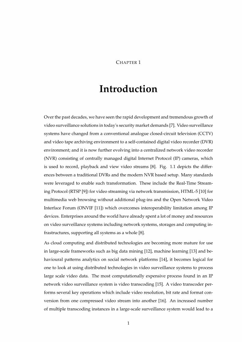
is used to record, playback and view video streams [8]. Fig. 1.1 depicts the differ-
ences between a traditional DVRs and the modern NVR based setup. Many standards
were leveraged to enable such transformation. These include the Real-Time Stream-
ing Protocol (RTSP [9]) for video streaming via network transmission, HTML-5 [10] for
multimedia web browsing without additional plug-ins and the Open Network Video
Interface Forum (ONVIF [11]) which overcomes interoperability limitation among IP
devices. Enterprises around the world have already spent a lot of money and resources
on video surveillance systems including network systems, storages and computing in-
frastructures, supporting all systems as a whole [8].
As cloud computing and distributed technologies are becoming more mature for use
in large-scale frameworks such as big data mining [12], machine learning [13] and be-
havioural patterns analytics on social network platforms [14], it becomes logical for
one to look at using distributed technologies in video surveillance systems to process
large scale video data. The most computationally expensive process found in an IP
network video surveillance system is video transcoding [15]. A video transcoder per-
forms several key operations which include video resolution, bit rate and format con-
version from one compressed video stream into another [16]. An increased number
of multiple transcoding instances in a large-scale surveillance system would lead to a
1
CHAPTER 1: INTRODUCTION
Figure 1.1: A typical setup example of DVRs versus the modern NVR
huge amount of CPU resources consumption, leaving limited available CPU resources
for the media server and web applications. Consequently, it slows down the overall
transcoding process. Therefore, a more cost-effective method for accessing computing
resources is required to realize multiple instances transcoding and speed up the over-
all performance of the video surveillance system. The remaining parts of this chapter
outlines the basic components of video processing which include video compression,
video data structures, video container formats and video streaming, from the acquisi-
tion of video sequences and transmission to display.
2
CHAPTER 1: INTRODUCTION
1.1 Background to the Media Content Delivery System
1.1.1 Video Acquisition, Pre-processing and Encoding
In a digital video coding system [17], a pool of video sequences is first captured by a
digital capture device such as a high resolution digital video camera. Pre-processing
operations are then performed on the raw uncompressed video frames to: 1) reduce
video resolution; and 2) correct and convert the color pixel format conforming to a cho-
sen standard. Next, an encoding process is carried out to transform the pre-processed
video sequences into coded bit-streams. The purpose of video encoding is to provide
a compact and bandwidth saving representation for the ease of network transmission
later.
1.1.2 Video Transmission, Decoding and Post-processing
Prior to transmitting video streams over a network, the coded bit-streams are packe-
tized into an appropriate transport format as prescribed by the chosen transport proto-
col, e.g. the Real-time Transport Protocol (RTP [18]). The transmission of video streams
involves client-server initiation, the receipt of video streams at the client side, as well
as, supported protocols, recovery of lost packets. At the client end, reconstructed video
sequences of the received bit-stream are achieved through a decoding process. On the
other hand, video encoding often adopts lossy compression in order to meet the tar-
geted transmission bandwidth constraint where the decoded video typically suffers
from quality degradation from the original video source as some reconstructed pixels
will be at best an approximation of the originals. If a lost packet fails to be recovered
during transmission, the decoder will apply an error concealment technique, focusing
on the recovery of the corrupted video frame. After decoding, post-processing opera-
tions are performed on reconstructed video sequences, which include color correction,
trimming and re-sampling. Finally, the video sequence is ready to be displayed. The
latency from decoding to display of the video sequences is one of the critical factors in
determining the viewing experiences of the viewers.
3
CHAPTER 1: INTRODUCTION
1.1.3 Fundamentals of Video Coding
The Structure of a Video Sequence
Video sequences basically are a series of time varying pictures, which are presented
with successive pictures in a constant time interval of milliseconds [19]. In order to
provide real-time video motions, a picture rate of at least 25 pictures per second is
required. The unit of picture rate is often referred to as frame rate (frames per second).
High definition captured videos found today can easily apply picture rates of 50 to 60
frames per second.
The Structure of a Coded Bit-stream
A video encoder basically transforms an input video sequence into coded bit-streams
which contain the essential information that is required to decode the bit-streams cor-
rectly and re-construct an approximation of the original video sequence for displaying
at the client side. A video encoding process involves applying compression to the video
source by eliminating redundancies found in the video sequence. A video sequence ba-
sically consists of two different types of redundancy: namely, the spatial and temporal
redundancies. The correlation presents between pixels within a video frame is known
as spatial redundancy. A video frame with the removal of such spatial redundancy that
is present within the frame is often named as an intra coded frame. On the contrary,
temporal redundancies are present between successive frames. Successive frames of a
sufficiently high frame rate video sequence are likely to be highly identical to one an-
other. Hence, the removal of such temporal redundancies involves between identical
successive frames in a video sequence is referred as Inter Coding. The spatial redun-
dancy of a frame is removed through the implementation of transform coding tech-
niques while temporal redundancies present between successive frames are discarded
through techniques of motion estimation and compensation [20].
IPB Frames in the GOP Structure
There are three common types of frames are adopted in video compression, namely:
the intra frame, predictive frame and bi-directional predictive frame [21]. In short, I
frames are also referred to as intra frames, while B and P are known as inter frames.
The repeated arrangement of such a collection of successive types of frames forms a
4
CHAPTER 1: INTRODUCTION
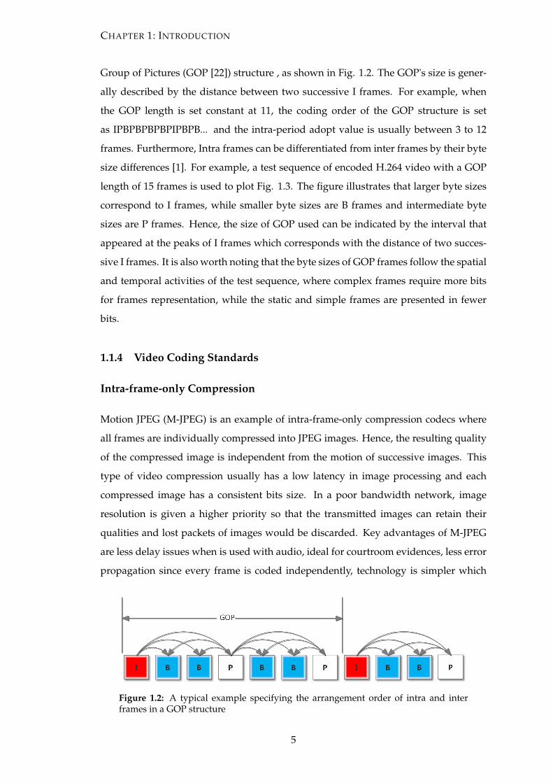
Group of Pictures (GOP [22]) structure , as shown in Fig. 1.2. The GOP's size is gener-
ally described by the distance between two successive I frames. For example, when
the GOP length is set constant at 11, the coding order of the GOP structure is set
as IPBPBPBPBPIPBPB... and the intra-period adopt value is usually between 3 to 12
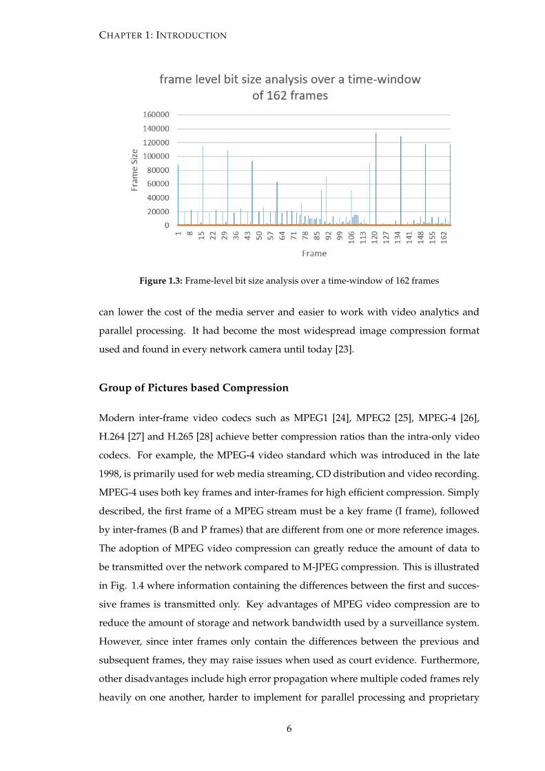
frames. Furthermore, Intra frames can be differentiated from inter frames by their byte
size differences [1]. For example, a test sequence of encoded H.264 video with a GOP
length of 15 frames is used to plot Fig. 1.3. The figure illustrates that larger byte sizes
correspond to I frames, while smaller byte sizes are B frames and intermediate byte
sizes are P frames. Hence, the size of GOP used can be indicated by the interval that
appeared at the peaks of I frames which corresponds with the distance of two succes-
sive I frames. It is also worth noting that the byte sizes of GOP frames follow the spatial
and temporal activities of the test sequence, where complex frames require more bits
for frames representation, while the static and simple frames are presented in fewer
bits.
1.1.4 Video Coding Standards
Intra-frame-only Compression
Motion JPEG (M-JPEG) is an example of intra-frame-only compression codecs where
all frames are individually compressed into JPEG images. Hence, the resulting quality
of the compressed image is independent from the motion of successive images. This
type of video compression usually has a low latency in image processing and each
compressed image has a consistent bits size. In a poor bandwidth network, image
resolution is given a higher priority so that the transmitted images can retain their
qualities and lost packets of images would be discarded. Key advantages of M-JPEG
are less delay issues when is used with audio, ideal for courtroom evidences, less error
propagation since every frame is coded independently, technology is simpler which
Figure 1.2: A typical example specifying the arrangement order of intra and interframes in a GOP structure
5
CHAPTER 1: INTRODUCTION
Figure 1.3: Frame-level bit size analysis over a time-window of 162 frames
can lower the cost of the media server and easier to work with video analytics and
parallel processing. It had become the most widespread image compression format
used and found in every network camera until today [23].
Group of Pictures based Compression
Modern inter-frame video codecs such as MPEG1 [24], MPEG2 [25], MPEG-4 [26],
H.264 [27] and H.265 [28] achieve better compression ratios than the intra-only video
codecs. For example, the MPEG-4 video standard which was introduced in the late
1998, is primarily used for web media streaming, CD distribution and video recording.
MPEG-4 uses both key frames and inter-frames for high efficient compression. Simply
described, the first frame of a MPEG stream must be a key frame (I frame), followed
by inter-frames (B and P frames) that are different from one or more reference images.
The adoption of MPEG video compression can greatly reduce the amount of data to
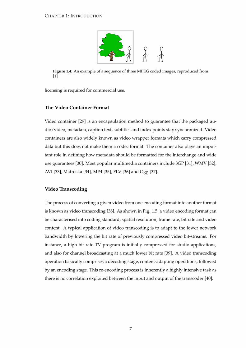
be transmitted over the network compared to M-JPEG compression. This is illustrated
in Fig. 1.4 where information containing the differences between the first and succes-
sive frames is transmitted only. Key advantages of MPEG video compression are to
reduce the amount of storage and network bandwidth used by a surveillance system.
However, since inter frames only contain the differences between the previous and
subsequent frames, they may raise issues when used as court evidence. Furthermore,
other disadvantages include high error propagation where multiple coded frames rely
heavily on one another, harder to implement for parallel processing and proprietary
6
CHAPTER 1: INTRODUCTION
Figure 1.4: An example of a sequence of three MPEG coded images, reproduced from[1]
licensing is required for commercial use.
The Video Container Format
Video container [29] is an encapsulation method to guarantee that the packaged au-
dio/video, metadata, caption text, subtitles and index points stay synchronized. Video
containers are also widely known as video wrapper formats which carry compressed
data but this does not make them a codec format. The container also plays an impor-
tant role in defining how metadata should be formatted for the interchange and wide
use guarantees [30]. Most popular multimedia containers include 3GP [31], WMV [32],
AVI [33], Matroska [34], MP4 [35], FLV [36] and Ogg [37].
Video Transcoding
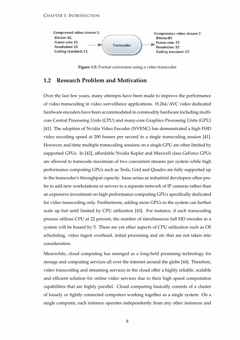
The process of converting a given video from one encoding format into another format
is known as video transcoding [38]. As shown in Fig. 1.5, a video encoding format can
be characterised into coding standard, spatial resolution, frame rate, bit rate and video
content. A typical application of video transcoding is to adapt to the lower network
bandwidth by lowering the bit rate of previously compressed video bit-streams. For
instance, a high bit rate TV program is initially compressed for studio applications,
and also for channel broadcasting at a much lower bit rate [39]. A video transcoding
operation basically comprises a decoding stage, content-adapting operations, followed
by an encoding stage. This re-encoding process is inherently a highly intensive task as
there is no correlation exploited between the input and output of the transcoder [40].
7
CHAPTER 1: INTRODUCTION
Figure 1.5: Format conversion using a video transcoder
1.2 Research Problem and Motivation
Over the last few years, many attempts have been made to improve the performance
of video transcoding in video surveillance applications. H.264/AVC video dedicated
hardware encoders have been accommodated in commodity hardware including multi-
core Central Processing Units (CPU) and many-core Graphics Processing Units (GPU)
[41]. The adoption of Nvidia Video Encoder (NVENC) has demonstrated a high FHD
video encoding speed at 200 frames per second in a single transcoding session [41].
However, real-time multiple transcoding sessions on a single GPU are often limited by
supported GPUs. In [42], affordable Nvidia Kepler and Maxwell class GeForce GPUs
are allowed to transcode maximum of two concurrent streams per system while high
performance computing GPUs such as Tesla, Grid and Quadro are fully supported up
to the transcoder's throughput capacity. Issue arises as industrial developers often pre-
fer to add new workstations or servers to a separate network of IP cameras rather than
an expensive investment on high performance computing GPUs specifically dedicated
for video transcoding only. Furthermore, adding more GPUs to the system can further
scale up but until limited by CPU utilization [43]. For instance, if each transcoding
process utilizes CPU at 22 percent, the number of simultaneous full HD encodes in a
system will be bound by 5. There are yet other aspects of CPU utilization such as OS
scheduling, video ingest overhead, initial processing and etc that are not taken into
consideration.
Meanwhile, cloud computing has emerged as a long-held promising technology for
storage and computing services all over the internet around the globe [44]. Therefore,
video transcoding and streaming services in the cloud offer a highly reliable, scalable
and efficient solution for online video services due to their high speed computation
capabilities that are highly parallel. Cloud computing basically consists of a cluster
of loosely or tightly connected computers working together as a single system. On a
single computer, each instance operates independently from any other instances and
8
CHAPTER 1: INTRODUCTION
therefore all computers working together can provide the advantages of powerful par-
allel computing capabilities. Since computing nodes can be heterogeneous, the cloud
computing platform becomes relatively inexpensive and therefore has an easily ex-
pandable cluster size. In order to improve such high efficiency of distributed comput-
ing and minimize the overall response time of tasks, authors in [45] had proposed the
most popular distributed computing paradigm, named MapReduce. In this paradigm,
computing efficiency of the system has been improved via load balancing on all com-
puting nodes which is, splitting the input data into key/value pairs and handle them
in a distributed manner. Hadoop [46], or more specifically the MapReduce framework,
is originally designed as a batch-oriented processing algorithm which focuses on opti-
mizing the overall completion time for batches of parallel transcoding tasks [47]. Video
transcoding in such architectures is not designed to work on-the-fly which means users
cannot start viewing the video as soon as the first video segment is transcoded and re-
ceived.
Another issue arises when the batch processing approach is attempted on hadoop het-
erogeneous platforms. Taking data locality into account when handling multiple input
files can greatly reduce the amount of network traffic generated between compute in-
stances. The current Hadoop block placement policy assumes that the homogeneity
nature of computing nodes always holds in a Hadoop cluster. In launching specula-
tive map tasks, data locality has not been taken into consideration as it is assumed that
the data is mostly available locally to mappers. The initial data placement algorithm
proposed in [48] begins by first splitting a large input file into even-sized chunks. The
data placement algorithm then schedules the sharded chunks to the cluster according
to the node’s data processing speed. Regardless of heterogeneity in node's process-
ing capacity, the initial data placement scheme distributes input chunks evenly so that
all nodes can have their local data to be processed within almost the same comple-
tion time. In the case of an over-utilized node, file chunks are repeatedly moved by
the data distribution server from an over-utilized node to an under-utilized node until
the workload is fairly distributed. Thus, their proposed data placement scheme adap-
tively distributes the amount of data stored evenly in each node in order to achieve an
improved data-processing speed while maintaining the initial data locality. However,
this method is not suitable for dynamic resource-aware task allocation via video con-
tent due to corrupted video frames acquired when video chunks are stored as HDFS
blocks. Also, video chunks re-distribution approaches do not distribute fairly enough
9
CHAPTER 1: INTRODUCTION
as the reconstructed batches of video chunks are much bigger blocks than a few dozen
of video frames found in a GOP structure.
Apart from difficulty in taking advantage of data locality during task re-allocation for
heterogeneous systems, Hadoop distributes worker slots by the amount set in static
configuration and will never be changed when the batch job is running. To address
this issue, a data pre-fetching mechanism proposed by [49] can be used to pre-fetch
the data to the corresponding under-utilized compute nodes in advance. The basic
idea of the data pre-fetching mechanism is to overlap data transmission with data pro-
cessing. In this way, when the input data of a map task is not available locally, the
overhead of data transmissions is hidden. However, a highly coordinated approach
is needed between the scheduling algorithm and the data pre-fetching mechanism for
task re-allocation. For this reason, we prefer stream processing over the batch dis-
tributed approach when furthering our future study on dynamic resource allocation
for distributing video transcoding in a heterogeneous computing environment.
1.3 Research Objective
The main research objective of this thesis is to investigate the existing parallel comput-
ing infrastructures, how they are being implemented from the point of view of stream
processing and batch processing, followed by proposing a method or architecture on
how to implement video streams transcoding on such infrastructures in an efficient
manner. The investigation will begin with comparative studies and a search for the
required system components. In addition to this, a baseline version of such systems
needs to be implemented on a related work, selecting a big data processing platform
for the purpose of experimentation, comparative studies, performance analysis of sys-
tem components and the proposed system as a whole.
1.4 Significant of Research
Many public cloud video transcoding platforms found today do not offer the real-time
requirement in producing transcoded video file or streams that are accessible on-the-
fly while transcoding. The real-time capability of the proposed system has enabled
distributed live transcoding to be realized on a larger scale, without having to wait for
the entire transcoding process to complete. Meanwhile, dedicated standalone compute
10
CHAPTER 1: INTRODUCTION
instances found in the public cloud market are scaled on an on-demand basis. Such a
single-tenancy approach would become costly for small and medium-sized enterprises
to transcode videos at a larger scale. Thus, a shared or multi-tenancy architecture in
providing such cloud video transcoding services is desired and can be facilitated by us-
ing the large scale and flexible data aggregation capabilities in Apache Storm. The main
idea is to allow clients to contribute an affordable number of cloud compute instances
to the cluster managed by our proposed system. An expanding cluster of such systems
enables a cost effective way to share a collection massive transcoding resources among
all clients. This is achieved by having the cluster’s resources to be shared among all
clients where compute resources utilization can be maximized during idle or off-peak
hours. In other words, online customer communities can leverage the unused resource
availability of the remaining shared systems onto their transcoding processes. In pri-
vate cloud applications, a resource-aware allocation scheme would play an important
role in distributing workloads fairly among heterogeneous cloud computing instances
in a company's private data center.
1.5 Thesis Contributions
The thesis has contributed to the design of a method for transcoding streaming videos
based on a big data processing platform. More specifically, a large-scale video transcod-
ing platform that is capable of distributedly transcode incoming live video streams in
real time has been realized in the course of the research. This has enabled the outcomes
of transcoded video streams to be accessible on-the-fly, and thereby facilitates users to
preview the content of the video output streams while transcoding, making sure the
desired quality is delivered. Secondly, impacts of data granularity on the proposed
real-time distributed video transcoding platform were studied and the best trade-off
between the load and communication overheads has allowed the parallel computers
to perform identically to their local baseline benchmarks which are to their maximum
computing capacities. Apart from that, a resource-aware task allocation scheme has
also been proposed for workload balancing by taking into consideration of the hetero-
geneous capabilities of computing nodes in a Storm cluster. This has enabled a fair
amount of sharded video streams to be allocated for each computer in accordance with
their computing ratios in real time.
11
CHAPTER 1: INTRODUCTION
1.6 Thesis Organization
This section gives a brief overview of chapter organization in this thesis. Chapter 2 will
investigate the related literature and studies that are relevant to the understanding of
development in parallel video transcoding. In Chapter 3, overviews of Apache Hadoop
and Apache Storm for data processing are introduced. After that, implementation of
the batch and real-time distributed video transcoding architectures are presented in
Chapter 4. Chapter 5 presents experiments and results obtained for related studies and
the proposed system. Last but not least, Chapter 6 summarizes the proposed methods
and results obtained in previous chapters along with some limitations, putting forward
some possible directions for future research.
12
CHAPTER 2
Literature Review
This chapter presents a wide range of relevant literatures on cost-efficient video transcod-
ing solutions. It includes ten sections. The first section describes the concept of hard-
ware efficiency for a multi-core processor in parallelizing the tasks of a H.264 encoder.
The second section presents another category of a many-core GPU in offloading por-
tions of the video transcoding tasks. The third section reviews the first commodity
hardware H.264 encoder released by Nvidia. In the fourth section, we explain the rea-
sons why the scalable video coding strategy is so well-known for simulcast applica-
tions by efficiently having the video transcoded once only. The fifth section discusses
the latest video coding standards available today. The sixth section covers the related
study of how video transcoding can be traded-off from the number of viewers in adap-
tive bit-rate streaming. The remaining sections investigate the state-of-the-art video
transcoding strategies in peer-to-peer systems, cloud services and distributed comput-
ing systems.
2.1 Specialized High-Performance Hardware Accelerators
Efficiency issues of general-purpose processors on multimedia applications, includ-
ing video decoding and encoding, have attracted a lot of research efforts. Various
approaches have been studied to improve hardware efficiency. Olli Lehtoranta et al.
[50] presented a scalable MPEG-4 hardware encoder for FPGA based Multiprocessor
System-on-Chip (MPSOC). Their results showed the scalability of their encoder frame-
work in MPSOC using horizontal spatial parallelism and the measured speed-up of
two and three encoding slaves are 1.7 and 2.3 times respectively. Xiao et al. [51] pro-
posed an on-chip distributed processing approach in parallelizing a baseline H.264 en-
13
CHAPTER 2: LITERATURE REVIEW
coder at the macroblock (16x16) and sub-macroblock (4x4) levels on a fine-grained of a
many-core processor. However, their works focus mainly on mapping the H.264 codec
to a many-core processor and energy efficiency for a single H.264 video encoding ses-
sion in real time. Although many approaches have been proposed to boost the speed
of a single video transcoding instance, a large-scale video transcoding system usually
experiences bottlenecks that are caused by the limited processing power of CPU when
multiple transcoding tasks are executed simultaneously.
2.2 Graphics Processing Units (GPUs)
More recent approach towards accelerating H.264/AVC is by parallel processing using
a many-core GPU. For example, the Nvidia CUDA Video Encoder (NVCUVENC), a
hybrid CPU/GPU accelerated H.264/AVC video encoder that leverages on hundreds
of CUDA cores in accelerating encoding tasks of NVCUVENC [52]. In another work,
Momcilovic et al. [53] proposed an efficient approach for collaborative H.264/AVC
inter-loop encoding in a heterogeneous CPU + GPU system. The integrated scheduling
and load balancing routines allow efficient distribution of workload among modules
across all processing units. In [54], Ko et al. proposed a novel motion estimation (ME)
algorithm implemented in a Nvidia GPU using sub-frame ME processing at frame-
level parallelization. However, these approaches have limited scalability issues: i.e
only a few GPUs can be employed and could not fully exploit capabilities of a multiple
GPUs system due to limitation bounded by CPU utilization.
2.3 The Nvidia Hardware Video Encoder
The emergence of dedicated hardware H.264/AVC encoders has recently accommo-
dated to commodity computing hardware such as CPUs and GPUs. In the past, hard-
ware video encoders were only commonly found in System-on-Chip (SoC) inside mo-
bile phones. These hardware encoders are often limited only to the built-in cameras
on mobile devices for video compression. On the other hand, hardware video en-
coders found in the video broadcasting industry are often expensive and do not pro-
vide enough flexibility in encoding parameters [41].
The first commodity hardware H.264 encoder was introduced and released along with
the Kepler GPU architecture by Nvidia in 2012. The first generation of the Nvidia HW
14
CHAPTER 2: LITERATURE REVIEW
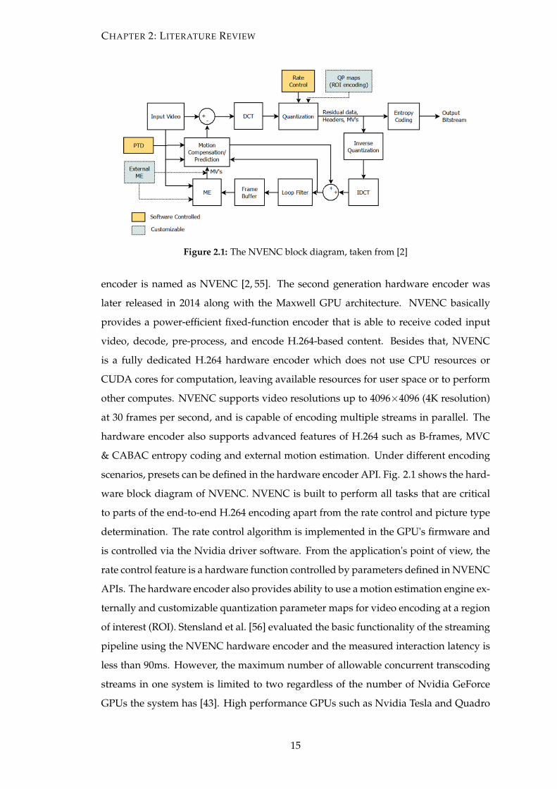
Figure 2.1: The NVENC block diagram, taken from [2]
encoder is named as NVENC [2, 55]. The second generation hardware encoder was
later released in 2014 along with the Maxwell GPU architecture. NVENC basically
provides a power-efficient fixed-function encoder that is able to receive coded input
video, decode, pre-process, and encode H.264-based content. Besides that, NVENC
is a fully dedicated H.264 hardware encoder which does not use CPU resources or
CUDA cores for computation, leaving available resources for user space or to perform
other computes. NVENC supports video resolutions up to 4096×4096 (4K resolution)
at 30 frames per second, and is capable of encoding multiple streams in parallel. The
hardware encoder also supports advanced features of H.264 such as B-frames, MVC
& CABAC entropy coding and external motion estimation. Under different encoding
scenarios, presets can be defined in the hardware encoder API. Fig. 2.1 shows the hard-
ware block diagram of NVENC. NVENC is built to perform all tasks that are critical
to parts of the end-to-end H.264 encoding apart from the rate control and picture type
determination. The rate control algorithm is implemented in the GPU's firmware and
is controlled via the Nvidia driver software. From the application's point of view, the
rate control feature is a hardware function controlled by parameters defined in NVENC
APIs. The hardware encoder also provides ability to use a motion estimation engine ex-
ternally and customizable quantization parameter maps for video encoding at a region
of interest (ROI). Stensland et al. [56] evaluated the basic functionality of the streaming
pipeline using the NVENC hardware encoder and the measured interaction latency is
less than 90ms. However, the maximum number of allowable concurrent transcoding
streams in one system is limited to two regardless of the number of Nvidia GeForce
GPUs the system has [43]. High performance GPUs such as Nvidia Tesla and Quadro
15
CHAPTER 2: LITERATURE REVIEW
Figure 2.2: Adaptive scalable video coding for simulcast applications, taken from [3]
do not have this limitation but they are too expensive for deployment in most cases.
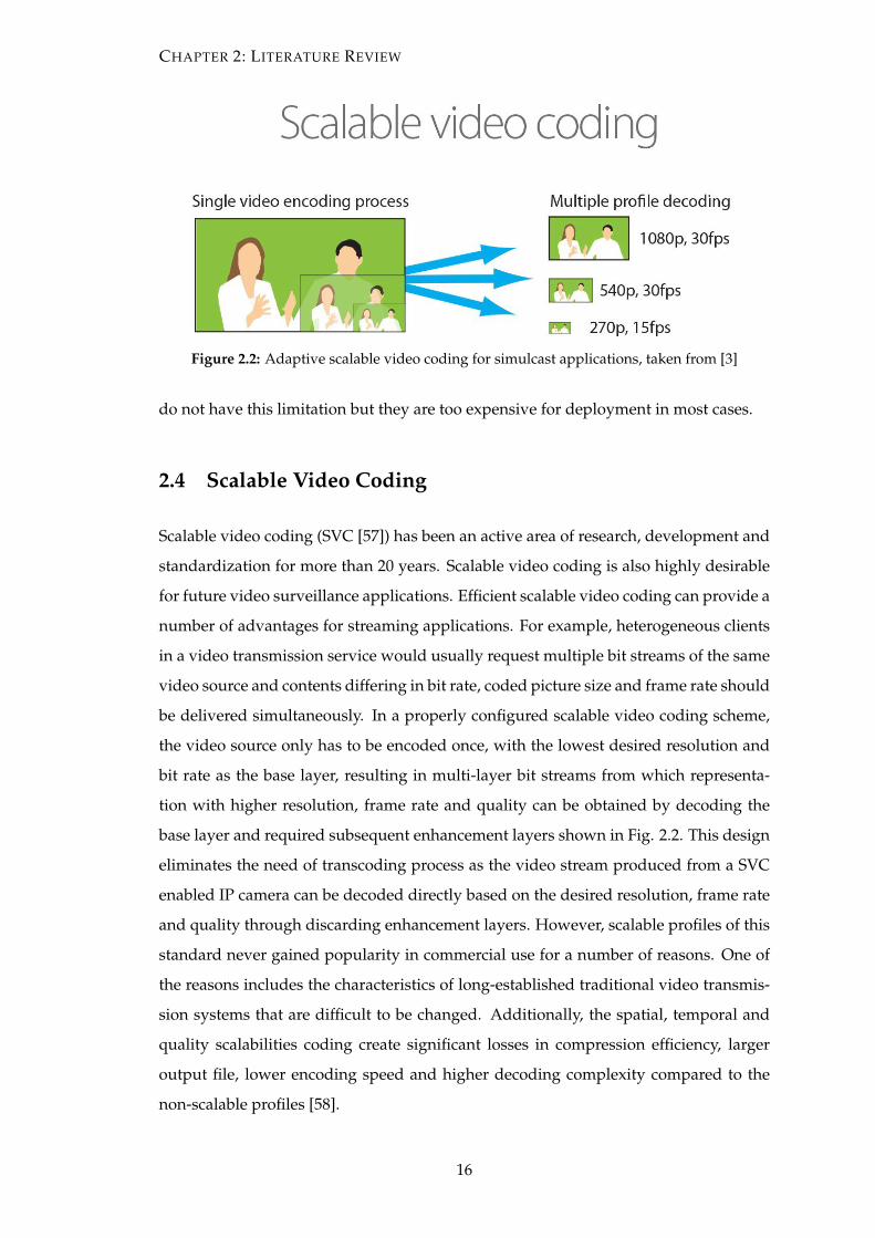
2.4 Scalable Video Coding
Scalable video coding (SVC [57]) has been an active area of research, development and
standardization for more than 20 years. Scalable video coding is also highly desirable
for future video surveillance applications. Efficient scalable video coding can provide a
number of advantages for streaming applications. For example, heterogeneous clients
in a video transmission service would usually request multiple bit streams of the same
video source and contents differing in bit rate, coded picture size and frame rate should
be delivered simultaneously. In a properly configured scalable video coding scheme,
the video source only has to be encoded once, with the lowest desired resolution and
bit rate as the base layer, resulting in multi-layer bit streams from which representa-
tion with higher resolution, frame rate and quality can be obtained by decoding the
base layer and required subsequent enhancement layers shown in Fig. 2.2. This design
eliminates the need of transcoding process as the video stream produced from a SVC
enabled IP camera can be decoded directly based on the desired resolution, frame rate
and quality through discarding enhancement layers. However, scalable profiles of this
standard never gained popularity in commercial use for a number of reasons. One of
the reasons includes the characteristics of long-established traditional video transmis-
sion systems that are difficult to be changed. Additionally, the spatial, temporal and
quality scalabilities coding create significant losses in compression efficiency, larger
output file, lower encoding speed and higher decoding complexity compared to the
non-scalable profiles [58].
16
CHAPTER 2: LITERATURE REVIEW
2.5 Latest Video Coding Standards
Video coding standards have been evolved from the well-known H.262/MPEG-2 stan-
dard [59] to H.264 Advanced Video Coding (AVC) [27]; and now to the emergence of
H.265 High-Efficiency Video Coding (HEVC) [28] and VP9 [60]. The H.264/MPEG-
AVC standard has been successfully satisfied the growing need for higher coding ef-
ficiency in standard-definition videos where an increase of about 50% in coding ef-
ficiency has been achieved compared to its predecessor H.262. However, both these
video coding standards were not designed for High Definition and Ultra High Def-
inition video content in the first place, the demand which is expected to be dramat-
ically increased in the near future. Consequently, the H.265/MPEG-HEVC standard
has emerged and to be applied to almost all existing H.264 applications which em-
phasize high-resolution video coding. Substantial bit-rate saving is achieved in H.265
encoding for the same visual quality when compared to its predecessor H.264. At the
same time, a few companies have also developed their own video codecs, which often
were kept secretly and partly on the variants of the state-of-the-art technologies used
in their standardized counterparts. One of these kinds of proprietary video codecs is
the VP8 codec [61], which was developed privately by On2 Technologies Inc and was
later acquired by Google. Based on VP8, Google started the development of its succes-
sor VP9 [60] in 2011, which was recently announced to be finalized. Grois et al. [62]
presented a performance comparison between H.265, H.264 and VP9. The HEVC en-
coder provides significant gains in terms of coding efficiency compared to both VP9
and H.264 encoders. On the other hand, the average encoding time of VP9 is more
than 100 times slower than the H.264 encoders and 7.35 times slower than H.265 en-
coders.
2.6 Adaptive Bit-rate Video Streaming
Over past few years, adaptive bit rate (ABR [63]) techniques have been deployed by
content providers to cope with the increased heterogeneity of network devices and con-
nections, for instance mobile phones with 3G/4G networks, tablets on Wi-Fi, laptops
and network TV channels. This technique consists of delivering multiple video rep-
resentations and is being applied to live streams in video surveillance systems. How-
ever, only a limited number of video channels are dedicated to the employment of ABR
17
CHAPTER 2: LITERATURE REVIEW
streaming in the streaming service system. In a large-scale live video streaming plat-
form such as Twitch, a huge amount of commodity servers used in the data center has
brought new issues in serving a large number of concurrent video channels. For each
video channel, a raw live video source is transcoded into multiple streams at different
resolutions and bit rates. These transcoding processes consume many computing re-
sources which induce significant costs, especially those dealing with a large number
of concurrent video channels. On the other hand, clients can be benefited from the
improvement of QoE by the reduction of delivery bandwidth costs. Aparicio-Pardo
et al. [64] proposed a better understanding on how viewers could benefits from ABR
streaming solutions by trading-offs video transcoding in ABR streaming solutions. This
is done by filtering out broadcasters and only those who can provide their own raw live
videos at all resolutions (480p, 720p and 1080p) are considered as candidates for ABR
streaming. Apart from that, candidate broadcasters with a minimum of N viewers are
only be selected for transcoding. This approach can satisfy a time varying demand
by efficiently exploiting an almost constant amount of computing resources without
wasting resources for streaming channels without many viewers.
2.7 Peer-Assisted Transcoding
Since the emergence of peer-to-peer (P2P) networking in recent years, there are some
study of literatures on transcoding techniques utilized in a P2P streaming system.
In [65, 66], Ravindra et.al and Yang et.al have proposed a P2P video transcoding archi-
tecture on a media streaming platform in which transcoding services are coordinated
to convert the streaming content into different formats in a P2P system. Liu et.al. [67]
proposed a peer-assisted transcoding system working on effective online transcoding
and ways to reduce the total computing overhead and bandwidth consumptions in P2P
networks. However, large-scale video transcoding application poses high requirement
of CPU and network I/O that incorporated with the unreliability low availability of
P2P clients makes it difficult to envision a practical implementation of such systems.
2.8 Cloud Video Transcoding
A cloud computing system basically comprises a computing resources infrastructure
that is made available to the end consumer. Cloud computing has been known for its
18
CHAPTER 2: LITERATURE REVIEW
powerful and cost-effective resources compared to those provided by their own single
machine system. Such high resource availability can be provided on a service-based
web interface where consumers can access the available resources in an on-demand
manner, reducing the hardware and maintenance costs to one usage-based billing. By
applying this utility-computing concept where computing resources are consumed in
the same way as electricity would, huge commercial endeavours like Google Cloud
Platform [68], Amazon Web Services [69], Microsoft Cloud [70], Linode [71], AliCloud
[72] and Telestream Cloud [73] were set up [74]. Li et al. [75] introduced a system
using cloud transcoding to optimize video streaming services for mobile devices. Video
transcoding on a cloud platform is a good solution to transcode a large volume of video
data because of its high throughput capacity. Netflix has [76] also deployed their video
transcoding platform on Amazon’s cloud services.
2.9 Video Transcoding using a Computer Cluster
Another widely researched area in speeding up the video transcoding process is the use
of computer clusters or also well known as the distributed computing platform. My-
oungjin Kim et al., Haoyu et al., Schmidt et al. and etc [77–87] have implemented a dis-
tributed video transcoding system using the popular MapReduce framework running
on top of the Hadoop Distributed File System (HDFS). Myoungjin et al.’s proposed dis-
tributed video transcoding system provides an excellent performance of 33 minutes in
completing the transcoding process in 50 gigabytes of video data set conducted on a
28 nodes HDFS cluster. Besides that, Rafael et al. [88] has demonstrated that by scaling
up the split and merging architectures with in-between key-frames of fixed 250 frames
chunk per worker, a fixed encoding time is guaranteed among workers independently
of the size of the input video. This allows total elasticity where it is possible to add and
remove workers on-the-fly according to demand. Hence, the cost of operation of the
public cloud service is thus minimal. On the other hand, Horacio et al. [89] has showed
that under overloaded condition, an increased number of split tasks produced from a
naive scheduler would result in a longer completion time than those non-split cases.
This indicates that further study on the distributed scheduling strategy is required to
fully accommodate available worker resources to task allocation.
However, these approaches are all batch-oriented which means they are not suitable for
continuous and real-time processing whenever a new data is produced continuously
19
CHAPTER 2: LITERATURE REVIEW
especially video data.
2.10 Resource-Aware Scheduling in a Distributed Heterogeneous
Platform
The heterogeneity of data processing clusters has become relatively common in com-
putational facilities. Polo, Jorda, et al. [90] presented a novel resource-aware adaptive
scheduler working on resource management and job scheduling for MapReduce. The
author’s technique leverages job profiling information in order to adjust the number
of slots dynamically on every machine, as well as workload scheduling across het-
erogeneous cluster to maximize resource utilization of the whole cluster. Boutaba et
al. [91] have analyzed various types of heterogeneity challenges in cloud computing
systems in terms of distribution of job lengths and sizes, the burstiness of job arrival
rates and heterogeneous resource requirements of the job. Ahmad et al. [92] proposed
Tarazu which achieves an overall speed up of 40% over Hadoop, incorporated with
communication-aware load balancing in scheduling of map jobs and predictive load-
balancing of reduce jobs. Rychly and Marek [93] proposed a Storm scheduler which
utilizes both the offline decision derived from results of the performance test and of
the performance captured online to re-schedule processors deployment based on ap-
plication needs. However, many of these approaches focus mainly on deployment and
scheduling of resources for job execution (spouts and bolts in Storm). They do not con-
sider the amount of tasks (task/tuple allocation in Storm) processed per resource based
on computing ratios.
20
CHAPTER 3
Apache Hadoop and Storm: The
Batch and Real-time Big Data
Processing Infrastructure
Over the past decade, the world has seen a revolution in large-scale data processing.
MapReduce over Hadoop [94], HDFS [95] and Spark related technologies have made
the possibility of storing big data economically and processing data distributed at vol-
ume that was previously unthinkable scale. This chapter explains the various essential
components of Hadoop: the architecture of the hadoop distributed file system, MapRe-
duce job, data locality and the handling of data in computation and machine failures.
Hadoop is one of the state-of-the-art batch processing framework used by many for
large-scale video transcoding, that is closely related to our work. In order to meet the
baseline requirement of our proposed method, Hadoop is used as a comparative study
to our work. Unfortunately, these batch oriented data processing technologies do not
possess real-time processing capabilities. There is no other way that Hadoop can turn
into a real-time system; real-time data processing requires fundamentally new require-
ment sets compared to batch processing [96]. There is a number of popular stream
processing platforms currently available such as Storm, Samza, Spark Streaming and
Flink. All of them offer exciting capabilities and appear promising. However, based on
the time factor, we chose to narrow down the detailed evaluation candidate to Storm
only. The remaining of this chapter explains the significant components of Storm, its
processing semantics, how Storm provides mechanisms to guarantee fault tolerance,
followed by metrics visualization in Storm, isolation scheduler and its benefits in video
transcoding.
21
CHAPTER 3: APACHE HADOOP AND STORM: THE BATCH AND REAL-TIME BIG DATA
PROCESSING INFRASTRUCTURE
3.1 Apache Hadoop: A Batch Processing Infrastructure
3.1.1 A Distributed Storage System in the Batch Processing Infrastructure
The core component of Apache Hadoop project comprises a file storage system that
is used to store data reliably and provide high throughput access to application data,
known as the Hadoop Distributed File System or HDFS [4]. The main idea is to split
the data into blocks and store them across multiple computers known as the HDFS
cluster. When it comes to processing the data, it is done exactly where its blocks are
stored. Rather than retrieving the data over the network from a central server, it is al-
ready in the cluster and ready to be processed on site. When the volume of data that
has to be stored in HDFS grows, users can always increase the cluster size by adding
more machines needed to the cluster. Ever since Hadoop has started gaining its popu-
larity, many other software applications have been built upon Hadoop. These software
applications are also collectively grouped within the Hadoop Ecosystem which was in-
tended to facilitate the data uploading process to the Hadoop cluster. Presently, there
are many ecosystems and projects that can communicate with each other to simplify
the installation process, thus maintaining the cluster. Cloudera, the company that has
put together the distribution of Hadoop called cloudera distribution or CDH which
integrates all key ecosystems along with Hadoop itself and packages them together so
that installation can be done easily.
3.1.2 The Hadoop Distributed File System
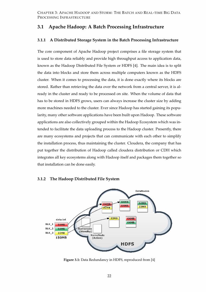
Figure 3.1: Data Redundancy in HDFS, reproduced from [4]
22
CHAPTER 3: APACHE HADOOP AND STORM: THE BATCH AND REAL-TIME BIG DATA
PROCESSING INFRASTRUCTURE
Fig. 3.1 illustrates the architecture of the reliable scalable data storage (HDFS) in Hadoop.
When a file is uploaded into HDFS, it is sharded into small chunks known as blocks.
Each block has a default size of 64MB and is given a unique label. As the file is up-
loaded to HDFS, each block will be stored on one of the DataNode in the hadoop clus-
ter. In order to identify which necessary blocks are required to re-construct the original
file, a NameNode is used to store this information as metadata. Apart from that, data
can be lost during network failures among the nodes and disk failure on an individ-
ual DataNode. To address these issues, Hadoop replicates each block three times and
stores them in HDFS. If a single node fails, there are two other copies of the block
on other nodes. In the case of under-replicated blocks, the NameNode will replicate
those blocks onto the cluster. In the past, NameNode was the single point of failure in
Hadoop. If the NameNode dies, the entire cluster is inaccessible as the metadata on the
NameNode is lost completely, so too the entire cluster data. Even the cluster has the
replicas of all blocks in DataNodes, there is no way of knowing which block belongs
to which file without the metadata. To avoid this problem, NameNode is configured
to store the metadata not only on the local drive but also in the network. These days,
NameNode is no longer a single point of failure in most production clusters as two
NameNodes are configured. The active NameNode works like before and the standby
NameNode can be configured to take over when the active NameNode has failed.
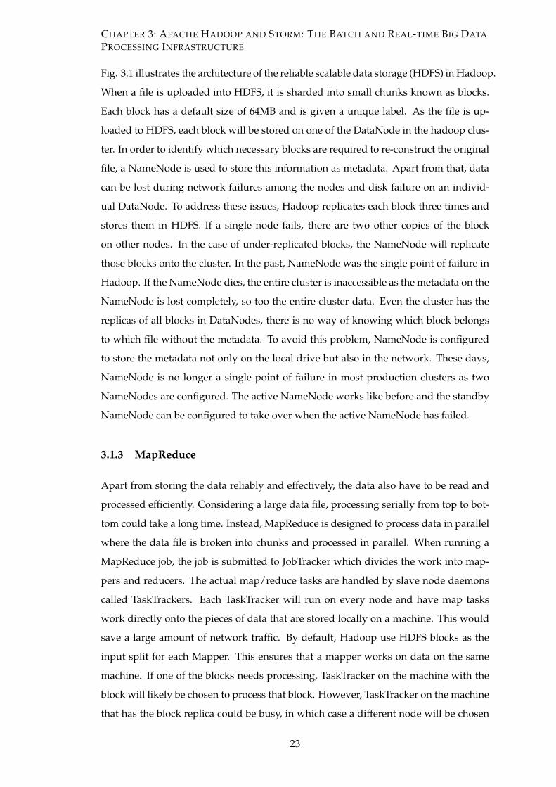
3.1.3 MapReduce
Apart from storing the data reliably and effectively, the data also have to be read and
processed efficiently. Considering a large data file, processing serially from top to bot-
tom could take a long time. Instead, MapReduce is designed to process data in parallel
where the data file is broken into chunks and processed in parallel. When running a
MapReduce job, the job is submitted to JobTracker which divides the work into map-
pers and reducers. The actual map/reduce tasks are handled by slave node daemons
called TaskTrackers. Each TaskTracker will run on every node and have map tasks
work directly onto the pieces of data that are stored locally on a machine. This would
save a large amount of network traffic. By default, Hadoop use HDFS blocks as the
input split for each Mapper. This ensures that a mapper works on data on the same
machine. If one of the blocks needs processing, TaskTracker on the machine with the
block will likely be chosen to process that block. However, TaskTracker on the machine
that has the block replica could be busy, in which case a different node will be chosen
23
CHAPTER 3: APACHE HADOOP AND STORM: THE BATCH AND REAL-TIME BIG DATA
PROCESSING INFRASTRUCTURE
Figure 3.2: Daemons of a MapReduce job, reproduced from [4]
to process the block and the block will be stream over the network. This is illustrated
in Fig. 3.2. In brief, mappers read data from inputs, produce an intermediate data and
pass to the reducers.
3.1.4 Data Locality in the Hadoop Cluster
Data locality is defined as the ability to keep compute and storage close together in
different locality levels such as process-local, node-local, rack-local and etc [97]. Data
locality is one of the most critical factors considered at task scheduling in data parallel
systems. Intermediate data generated from map tasks are stored locally (not upload to
HDFS) so that data locality of map tasks is benefited. As such, MapReduce conserves
network bandwidth by taking the shortest distance between computes and storages,
that is data blocks to be processed are selected nearest to the storage drives and the
compute instances of the machines that create the Hadoop cluster. For instance, the
MapReduce master node locates the input data and a machine that contains a replica
of the corresponding data block is to be scheduled to the map task. If such a task can
be found, node-level data locality benefits and no network bandwidth is consumed.
Otherwise, Hadoop will attempt to schedule a map task that is nearest to a replica of
that input data block to achieve rack-level data locality (the input data block and task
are randomly picked and dispatched). However, such data locality in Hadoop does not
consider other factors such as system load and fairness.
24
CHAPTER 3: APACHE HADOOP AND STORM: THE BATCH AND REAL-TIME BIG DATA
PROCESSING INFRASTRUCTURE
3.1.5 Fault-Tolerance
Since MapReduce processes terabytes or even petabytes of data on hundreds or thou-
sands of machines, it must be a fail-safe system [45]. In the following paragraph, we
discuss how Hadoop keeps data safe and resilient in case of worker and master failures.
Periodically, the master node checks for active connection with all workers. If a worker
fails to respond within a certain amount of time, the worker is marked failed by the
master node. Workers with their map tasks completed are restoring back to their idle
state, and these workers consecutively become available for re-scheduling. In a similar
way, when a worker fails, all map or reduce tasks in progress under the failed worker
node are terminated and therefore become eligible for re-scheduling onto other worker
nodes. Completed map tasks of a failed machine are inaccessible upon machine fail-
ures and therefore have to be re-executed as their outputs are locally stored on the
failed machine. On the other hand, the output of reduce tasks is stored globally so that
the completed reduce task does not need to be re-executed in case of machine failures.
When a worker fails, the map task is re-executed on another worker. Re-execution of
the map task will be notified to every reducer. Any reducers that do not receive the
notification message from the failed mapper will read from the re-allocated mapper.
Furthermore, MapReduce is resilient towards failures of large-scale workers. For in-
stance, network maintenance and updates of a running MapReduce cluster can cause
a cluster of 100 machines to become inaccessible for several minutes. In order to make
forward progress and complete MapReduce operations, the master node simply has to
re-execute the work completed by the inaccessible worker machine.
If the master daemon dies, a new copy of the master daemon is started over from the
last check-pointed state. However, even the master failure is unlikely where there is
only one master; the current implementation terminates MapReduce computation if
the master fails. Users would have to monitor for this failure and debug the MapRe-
duce operation if they needed to [45].
3.1.6 Task Granularity
In terms of task granularity, Hadoop’s map phase is subdivided into M chunks (typi-
cally 64MB) and the reduce phase into R chunks. The number for M and R is preferably
greater than the number of worker nodes. As such, all worker nodes can perform many
different tasks which then improve the dynamic of load balancing and speed up the re-
25
CHAPTER 3: APACHE HADOOP AND STORM: THE BATCH AND REAL-TIME BIG DATA
PROCESSING INFRASTRUCTURE
covery process in the case of workers failures. This is because the remaining map tasks,
given the fine granularity, can be more easily reallocated across all other worker ma-
chines. Since the master node must schedule the map and reduce tasks and store them
in memory in the first place, the implementation of MapReduce has practical bounds
on how numerous M and R can be. Additionally, R is often constrained by user’s pref-
erences because the output of multiple reduce tasks ends up with multiple output files.
Thus, M is tended to be chosen as task granularity so that every task is roughly 16MB
to 64MB of the input data (where throughput optimization is the most effective), and
R is a small multiple of the number of worker machines [45].
3.1.7 Discussion
There is a number of benefits Hadoop can provide for video transcoding. First, video
data can be stored reliably in HDFS. Due to its data locality design, Hadoop can pro-
vide high throughput video transcoding, maximizing the utilization of all computing
resources. Besides that, the Hadoop cluster can be easily scale based on resource de-
mand for video transcoding, eliminating the delay which is needed to re-run the whole
job. Apart from that, the Hadoop cluster can be easily deployed in available cloud
services such as the Amazon Elastic Compute Cloud (AWS EC2 [98]). However, cloud
compute instances are expensive to be deployed in a larger scale. The pricing rate
multiplied corresponding to the number of instances used in the Hadoop-based video
transcoding system.
26
CHAPTER 3: APACHE HADOOP AND STORM: THE BATCH AND REAL-TIME BIG DATA
PROCESSING INFRASTRUCTURE
3.2 Apache Storm: A Stream Processing Infrastructure
3.2.1 Big Data Processing in the Real-time Stream Processing Infrastructure
Big data is basically characterized into four dimensions, namely the volume, velocity,
variety and veracity of big data, and Hadoop-like frameworks handle the volume and
variety parts of big data [99]. Along with the volume and variety, a real-time system
requires handling the high velocity of processing, that is the velocity of data. And
maintaining the velocity of data in big data computation is a complicated task. First,
the system has to be able to gather data generated by real-time stream events which are
coming in the rate of millions of message streams per second. Even as the data is be-
ing gathered, the system has to be robust enough to process the data in parallel. Then
comes the complex task of performing event correlation and extracting meaningful in-
formation from these moving streams. All of these need to happen in a fault tolerant
and distributed manner. All employed real-time systems must be low latency systems,
enabling faster computation and facilitating near real-time response capabilities. Data
streams can be gathered from various sources, processed in the stream processing en-
gine, the result of which is written to a destination system. In between, queues are
used to store/buffer messages. Before Storm, one would need to build a network of
queues and workers manually to do data processing in real time. However, issues such
as tedious coding, poor fault-tolerance, data lost and painful to scale are limitations to
such naive approaches. This is where Storm comes into the picture.
Apache Storm is a big data framework fine-tuned to handle unbounded streams of data.
As mentioned, modern big data processing environments have evolved from batch
computing against large volumes of static data and now into real-time computing on
data streams that are produced in real time. This is especially important in social me-
dia platforms such as Twitter which requires making complex decisions based on the
data created by user interactions [5]. Storm includes multiple features such as horizon-
tal scalability, resilient, guaranteed data processing, extensibility and efficient as listed
below:
1) Scalable: Nodes can be added and removed non-disruptively without affecting the
uniform distribution of works.
2) Resilient: Fault-tolerance is essential for hardware failures and the continuation of
job execution if a slave node goes down.
27
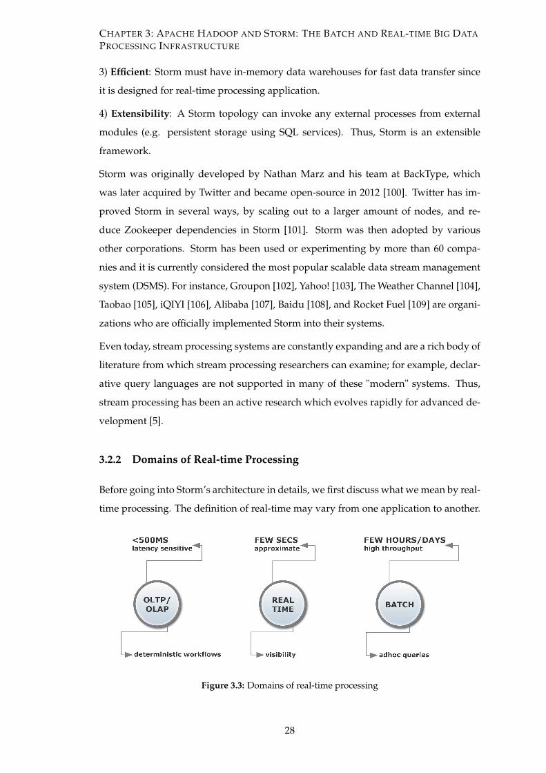
CHAPTER 3: APACHE HADOOP AND STORM: THE BATCH AND REAL-TIME BIG DATA
PROCESSING INFRASTRUCTURE
3) Efficient: Storm must have in-memory data warehouses for fast data transfer since
it is designed for real-time processing application.
4) Extensibility: A Storm topology can invoke any external processes from external
modules (e.g. persistent storage using SQL services). Thus, Storm is an extensible
framework.
Storm was originally developed by Nathan Marz and his team at BackType, which
was later acquired by Twitter and became open-source in 2012 [100]. Twitter has im-
proved Storm in several ways, by scaling out to a larger amount of nodes, and re-
duce Zookeeper dependencies in Storm [101]. Storm was then adopted by various
other corporations. Storm has been used or experimenting by more than 60 compa-
nies and it is currently considered the most popular scalable data stream management
system (DSMS). For instance, Groupon [102], Yahoo! [103], The Weather Channel [104],
Taobao [105], iQIYI [106], Alibaba [107], Baidu [108], and Rocket Fuel [109] are organi-
zations who are officially implemented Storm into their systems.
Even today, stream processing systems are constantly expanding and are a rich body of
literature from which stream processing researchers can examine; for example, declar-
ative query languages are not supported in many of these "modern" systems. Thus,
stream processing has been an active research which evolves rapidly for advanced de-
velopment [5].
3.2.2 Domains of Real-time Processing
Before going into Storm’s architecture in details, we first discuss what we mean by real-
time processing. The definition of real-time may vary from one application to another.
Figure 3.3: Domains of real-time processing
28
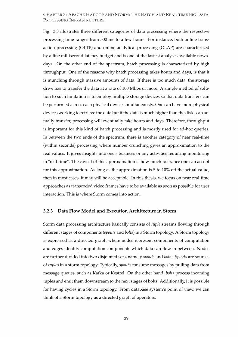
CHAPTER 3: APACHE HADOOP AND STORM: THE BATCH AND REAL-TIME BIG DATA
PROCESSING INFRASTRUCTURE
Fig. 3.3 illustrates three different categories of data processing where the respective
processing time ranges from 500 ms to a few hours. For instance, both online trans-
action processing (OLTP) and online analytical processing (OLAP) are characterized
by a fine millisecond latency budget and is one of the fastest analyses available nowa-
days. On the other end of the spectrum, batch processing is characterized by high
throughput. One of the reasons why batch processing takes hours and days, is that it
is munching through massive amounts of data. If there is too much data, the storage
drive has to transfer the data at a rate of 100 Mbps or more. A simple method of solu-
tion to such limitation is to employ multiple storage devices so that data transfers can
be performed across each physical device simultaneously. One can have more physical
devices working to retrieve the data but if the data is much higher than the disks can ac-
tually transfer, processing will eventually take hours and days. Therefore, throughput
is important for this kind of batch processing and is mostly used for ad-hoc queries.
In between the two ends of the spectrum, there is another category of near real-time
(within seconds) processing where number crunching gives an approximation to the
real values. It gives insights into one’s business or any activities requiring monitoring
in "real-time". The caveat of this approximation is how much tolerance one can accept
for this approximation. As long as the approximation is 5 to 10% off the actual value,
then in most cases, it may still be acceptable. In this thesis, we focus on near real-time
approaches as transcoded video frames have to be available as soon as possible for user
interaction. This is where Storm comes into action.
3.2.3 Data Flow Model and Execution Architecture in Storm
Storm data processing architecture basically consists of tuple streams flowing through
different stages of components (spouts and bolts) in a Storm topology. A Storm topology
is expressed as a directed graph where nodes represent components of computation
and edges identify computation components which data can flow in-between. Nodes
are further divided into two disjointed sets, namely spouts and bolts. Spouts are sources
of tuples in a storm topology. Typically, spouts consume messages by pulling data from
message queues, such as Kafka or Kestrel. On the other hand, bolts process incoming
tuples and emit them downstream to the next stages of bolts. Additionally, it is possible
for having cycles in a Storm topology. From database system’s point of view, we can
think of a Storm topology as a directed graph of operators.
29
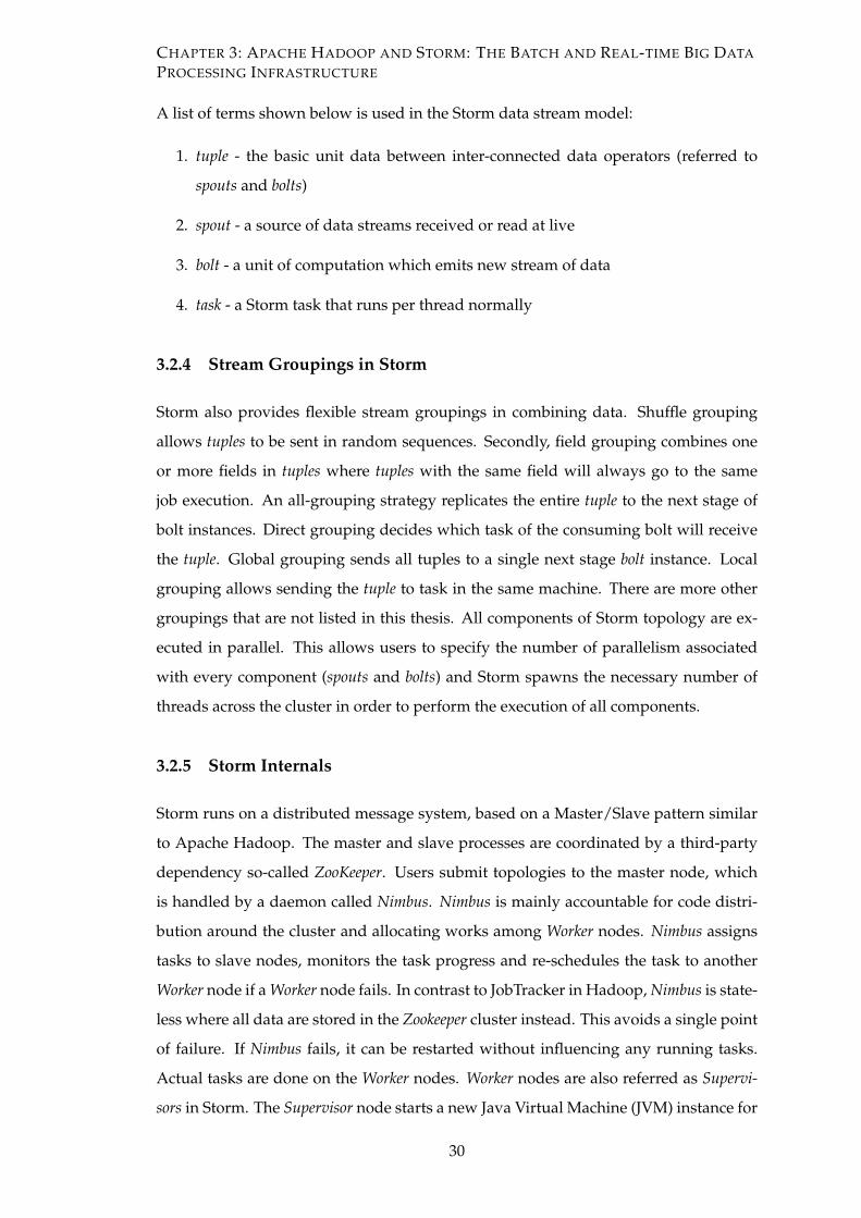
CHAPTER 3: APACHE HADOOP AND STORM: THE BATCH AND REAL-TIME BIG DATA
PROCESSING INFRASTRUCTURE
A list of terms shown below is used in the Storm data stream model:
1. tuple - the basic unit data between inter-connected data operators (referred to
spouts and bolts)
2. spout - a source of data streams received or read at live
3. bolt - a unit of computation which emits new stream of data
4. task - a Storm task that runs per thread normally
3.2.4 Stream Groupings in Storm
Storm also provides flexible stream groupings in combining data. Shuffle grouping
allows tuples to be sent in random sequences. Secondly, field grouping combines one
or more fields in tuples where tuples with the same field will always go to the same
job execution. An all-grouping strategy replicates the entire tuple to the next stage of
bolt instances. Direct grouping decides which task of the consuming bolt will receive
the tuple. Global grouping sends all tuples to a single next stage bolt instance. Local
grouping allows sending the tuple to task in the same machine. There are more other
groupings that are not listed in this thesis. All components of Storm topology are ex-
ecuted in parallel. This allows users to specify the number of parallelism associated
with every component (spouts and bolts) and Storm spawns the necessary number of
threads across the cluster in order to perform the execution of all components.
3.2.5 Storm Internals
Storm runs on a distributed message system, based on a Master/Slave pattern similar
to Apache Hadoop. The master and slave processes are coordinated by a third-party
dependency so-called ZooKeeper. Users submit topologies to the master node, which
is handled by a daemon called Nimbus. Nimbus is mainly accountable for code distri-
bution around the cluster and allocating works among Worker nodes. Nimbus assigns
tasks to slave nodes, monitors the task progress and re-schedules the task to another
Worker node if a Worker node fails. In contrast to JobTracker in Hadoop, Nimbus is state-
less where all data are stored in the Zookeeper cluster instead. This avoids a single point
of failure. If Nimbus fails, it can be restarted without influencing any running tasks.
Actual tasks are done on the Worker nodes. Worker nodes are also referred as Supervi-
sors in Storm. The Supervisor node starts a new Java Virtual Machine (JVM) instance for
30
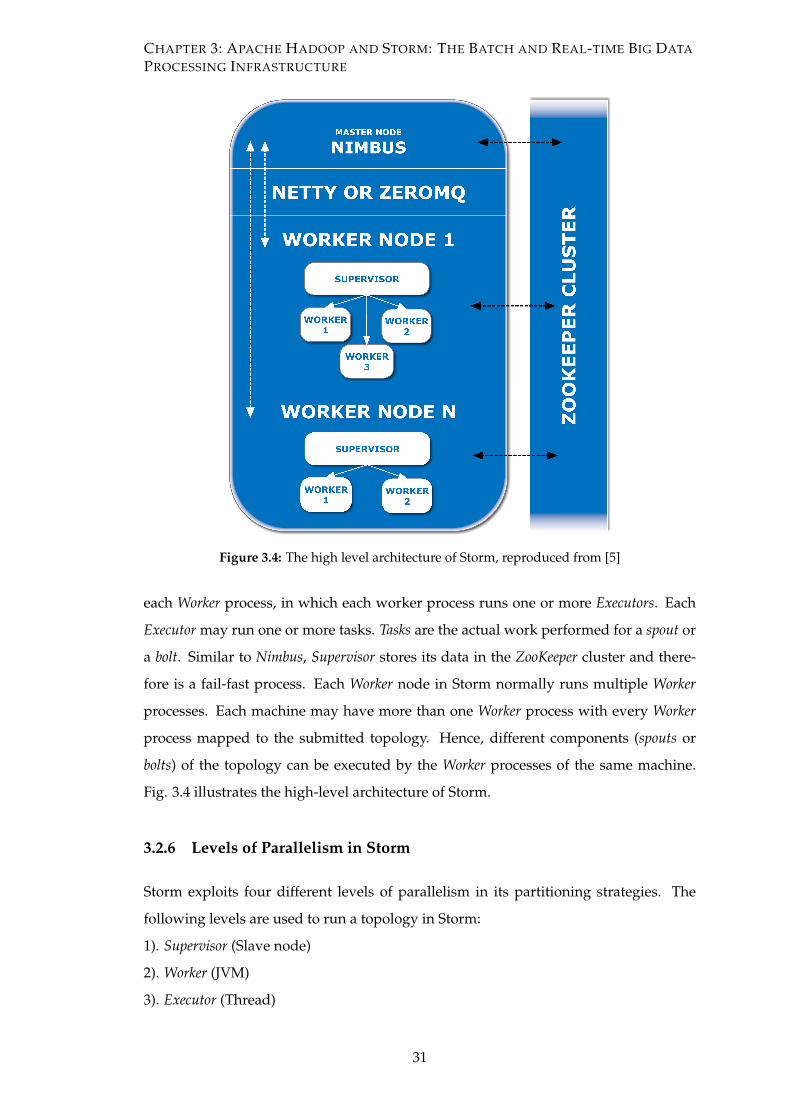
CHAPTER 3: APACHE HADOOP AND STORM: THE BATCH AND REAL-TIME BIG DATA
PROCESSING INFRASTRUCTURE
Figure 3.4: The high level architecture of Storm, reproduced from [5]
each Worker process, in which each worker process runs one or more Executors. Each
Executor may run one or more tasks. Tasks are the actual work performed for a spout or
a bolt. Similar to Nimbus, Supervisor stores its data in the ZooKeeper cluster and there-
fore is a fail-fast process. Each Worker node in Storm normally runs multiple Worker
processes. Each machine may have more than one Worker process with every Worker
process mapped to the submitted topology. Hence, different components (spouts or
bolts) of the topology can be executed by the Worker processes of the same machine.
Fig. 3.4 illustrates the high-level architecture of Storm.
3.2.6 Levels of Parallelism in Storm
Storm exploits four different levels of parallelism in its partitioning strategies. The
following levels are used to run a topology in Storm:
1). Supervisor (Slave node)
2). Worker (JVM)
3). Executor (Thread)
31
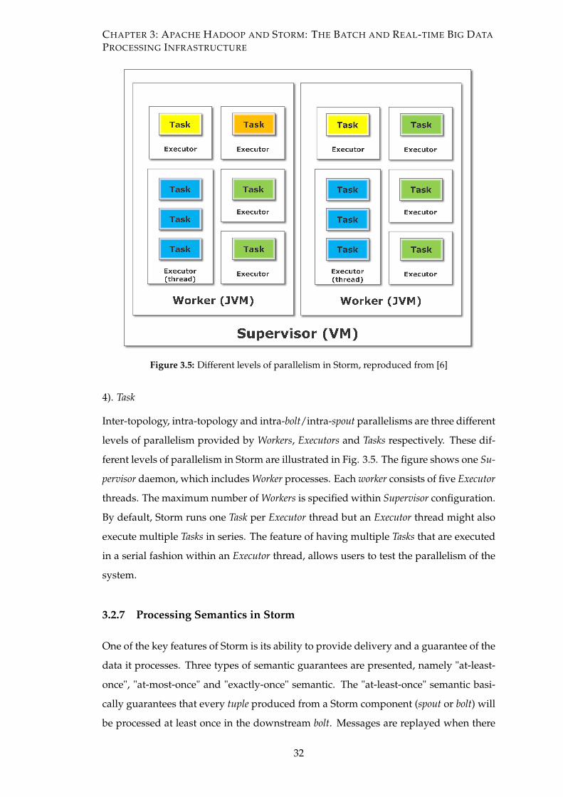
CHAPTER 3: APACHE HADOOP AND STORM: THE BATCH AND REAL-TIME BIG DATA
PROCESSING INFRASTRUCTURE
Figure 3.5: Different levels of parallelism in Storm, reproduced from [6]
4). Task
Inter-topology, intra-topology and intra-bolt/intra-spout parallelisms are three different
levels of parallelism provided by Workers, Executors and Tasks respectively. These dif-
ferent levels of parallelism in Storm are illustrated in Fig. 3.5. The figure shows one Su-
pervisor daemon, which includes Worker processes. Each worker consists of five Executor
threads. The maximum number of Workers is specified within Supervisor configuration.
By default, Storm runs one Task per Executor thread but an Executor thread might also
execute multiple Tasks in series. The feature of having multiple Tasks that are executed
in a serial fashion within an Executor thread, allows users to test the parallelism of the
system.
3.2.7 Processing Semantics in Storm
One of the key features of Storm is its ability to provide delivery and a guarantee of the
data it processes. Three types of semantic guarantees are presented, namely "at-least-
once", "at-most-once" and "exactly-once" semantic. The "at-least-once" semantic basi-
cally guarantees that every tuple produced from a Storm component (spout or bolt) will
be processed at least once in the downstream bolt. Messages are replayed when there
32
CHAPTER 3: APACHE HADOOP AND STORM: THE BATCH AND REAL-TIME BIG DATA
PROCESSING INFRASTRUCTURE
are failures. For at-most-once semantic, every tuple is processed once and dropped
in case of failures. Exactly-once semantic guarantees that no duplicated messages are
delivered to the processing bolts.
To provide "at-least-once" semantic, Storm topologies are augmented with "acker" bolts
that track tuples-tree for every tuple that is emitted by the spouts. Storm tagged every
processed tuple with a randomly generated unique 64-bit "message/tuple id". Trace
ids are then grouped together with tuples in spouts once the data streams are first pull
from the input sources. Whenever a tuple is processed, new tuple or multiple tuples can
be produced. For example, tuple containing the entire sentence is sharded into a set
of words by a bolt, producing new set of tuples: tuple of words and tuple of sequence
numbers from the input tuple of the sentence. Every produced tuple is then assigned to
a new random 64-bit id, and the list of new tuple ids that is associated with the output
tuples are retained in a provenance tree. Backflow mechanism is used to acknowledge
the tasks that have contributed to the output tuples when these tuples about to leave
the topology. In order to retire these tuples, the backflow mechanism reaches out to the
spouts that have already started processing tuples in the first place.
Exactly-once semantic in Storm can be achieved by transactional topology where strong
ordering of tuples can provide such capabilities. Each tuple is associated with a trans-
action id and is incremental with every tuple. If a tuple fails and needs to be replayed,
then it is re-emitted with the exact same transaction id.
3.2.8 Fault Tolerance Daemons in Storm
A Storm cluster has several different daemon processes: Nimbus that schedules jobs to
worker processes, Supervisors that start and kill Worker processes, the log viewer that
gives access to log files, and Storm UI that shows the status of a cluster. When a Worker
process dies, it is restarted by the Supervisor daemon. If failures are on the start-up
and heartbeats, Nimbus will re-schedule the Worker process to another machine. In the
mean time, tasks assigned on the failed machine will be timed-out and Nimbus will re-
assign those tasks to the new scheduled Worker. The Nimbus and Supervisor daemons
are supervised by daemon tools or monit so that if the Nimbus or Supervisor daemons
die, they will be backed-up as if nothing has happened. In addition, since all states are
stored in the Zookeeper cluster, the Nimbus and Supervisor daemons become fail-fast
and stateless.
33
CHAPTER 3: APACHE HADOOP AND STORM: THE BATCH AND REAL-TIME BIG DATA
PROCESSING INFRASTRUCTURE
Most notably, no running worker processes are affected by the death of Nimbus or
their Supervisors as cluster communication and heartbeats are all managed by the
Zookeeper cluster. This is in contrast to Hadoop where if a JobTracker dies, all run-
ning jobs are completely lost. Even if the Nimbus node is down, workers will still
continue to function and supervisors will continue to restart workers if the supervisor
daemon dies. However, if Nimbus goes down, workers cannot be reassigned to other
machines.
3.2.9 Daemon Metrics and Monitoring in Storm
Storm User Interface (UI) provides a web interface for visualization of running topol-
ogy; with a complete break-up of internal spouts and bolts. Storm UI also contributes
information regarding any errors coming in tasks and fine-grained stats on the through-
put and latencies of every component of the running topology. Storm UI helps in de-
bugging issues at high-level, for example as soon as an error happens in a topology,
a stack trace is displayed. The Storm’s built-in metrics feature provides framework-
level support for collecting and reporting metrics to external systems. Worker logs are
another source of valuable information used for troubleshooting any topology errors.
3.2.10 Auto Scaling in Storm
Storm supports configuring initial parallelism at various levels per topology; number
of worker processes, number of executors, number of tasks. Storm supports dynamic
re-balancing which allows increasing or decreasing the number of worker processes
and/or executors without restarting the cluster or the topology. Although the number
of executors for a component may change over time, the number of initial tasks con-
figured is always the same throughout the lifetime of a topology. Once all supervisor
nodes are fully saturated with worker processes and there is a need to scale out, one
simply has to begin a new supervisor node and pointing it to the Zookeeper cluster.
All resources on the newly added supervisor will then be available for scheduling. It
is possible to automate the logic of monitoring current resource consumption on each
node in the Storm cluster, and dynamically add more resources.
34
CHAPTER 3: APACHE HADOOP AND STORM: THE BATCH AND REAL-TIME BIG DATA
PROCESSING INFRASTRUCTURE
3.2.11 The Isolation Scheduler in Storm
Each worker process runs executors for a particular topology only where mixing of
different topology tasks is not allowed at worker process level. This provides topol-
ogy level run-time isolation. Furthermore, each executor thread runs one or more tasks
of the same component (spout or bolt) without mixing tasks across components. In
a shared cluster setup, a topology that needs a large number of tasks, and resources
(CPU cores, memory) can be submitted along with a smaller topology. To handle this,
the Storm's isolation scheduler provides multi-tenancy across topologies and avoids
shared-resource contention among topologies. It allows specifying which topology
should be isolated, that is run on a dedicated set of machines within a cluster. All
isolated topologies are given higher priority than non-isolated ones, taking resources
from the non-isolated.
3.2.12 Ease of Development in Storm
Storm provides a really simple, rich and intuitive API that simply describes the DAG
nature of processing flows (topology). Storm tuples, which provide the abstraction
of data flowing between nodes in the DAG, are dynamically typed. Developers can
start with writing topologies and run them in the local cluster mode or the pseudo-
distributed mode. In the local mode, threads are used to simulate worker nodes, al-
lowing developers to set breakpoints, halt execution, inspect variables, and profile their
topology before deploying it to the real cluster where all of this is much more difficult.
3.2.13 Discussion
There are a number of benefits Storm can provide for video transcoding. First, video
data can be gathered in terms of live video streams from IP cameras into the Storm
based data ingestion component called Spout. Due to its stream processing architecture,
the output from processing can be visualized on-the-fly, providing real-time transcoded
video streams ready to begin streaming to the client end. Since the input video stream
is distributed all over to the Storm cluster and all computers are utilized under the
proposed system, the CPU and memory usage of each computer can be reduced in real
time when the input data rate is lower than the total data processing rate. In the context
of a large-scale video transcoding system, more input video streams can be processed
35
CHAPTER 3: APACHE HADOOP AND STORM: THE BATCH AND REAL-TIME BIG DATA
PROCESSING INFRASTRUCTURE
in such system.
In cloud computing application, Storm can provide a shared video transcoding service
using the available public cloud services such as the Amazon Elastic Compute Cloud
(AWS EC2 [98]). Resource utilization of such shared cluster can be maximized for the
fact that not all clients are transcoding videos in a 24/7 basis. This allows idle clients
to share their available allocated compute resources to the cluster. In this way, on-
line clients can leverage resource availability of the remaining unused resources in the
shared cluster onto their transcoding processes.
An expanding cluster of such shared systems enables a cost effective way to share a
collection of massive transcoding resources among all customers by having customers
pay only for their contributed number of instances and charges for maintaining the
entire cluster. On the contrary, dedicated standalone instances in an on-demand basis
can cost a lot for a customer to transcode video at a larger scale.
36
CHAPTER 4
Distributed Video Transcoding on a
Selected Big Data Processing
Platform
Transcoding a large volume of daily recorded video files with a volume in terabytes or
petabytes gives rise to potential challenges in reducing the processing time. High cost
of reliable storages is needed to store the video reliably in traditional storage systems
and to stream the distributed data from traditional storage devices across the network
to the central processor, which can take up a long time and processing can be extremely
slow. When there are more cameras deployed along the way, more video streams are
needed to be stored. In order to store such a huge amount of videos, a way to easily
scale the video storage capacity up to a massive volume is required. The chapter first
presents the architecture of a Hadoop-based video transcoding system and its data
placement issues in heterogeneous systems. The remaining of this chapter presents
the architecture of the proposed Storm-based video transcoding system and its compo-
nents reflected in a Storm topology.
4.1 The Batch-oriented Distributed Video Transcoding Method
4.1.1 Adopting a Distributed File System in Storing Video Data
To store such a huge volume of video data reliably, the Hadoop Distributed File System
(HDFS) is adopted. HDFS is a fault-tolerant storage system, not only does it store
data in a distributed way across multiple machines and scales up incrementally, it also
37
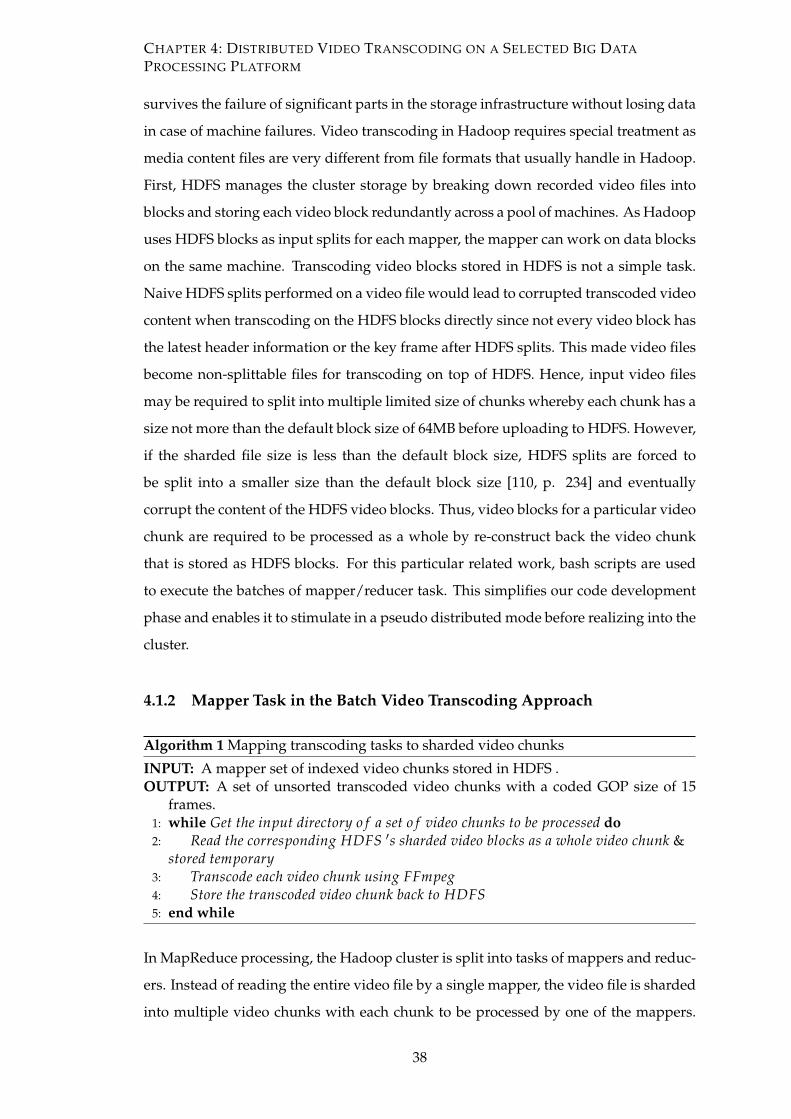
CHAPTER 4: DISTRIBUTED VIDEO TRANSCODING ON A SELECTED BIG DATA
PROCESSING PLATFORM
survives the failure of significant parts in the storage infrastructure without losing data
in case of machine failures. Video transcoding in Hadoop requires special treatment as
media content files are very different from file formats that usually handle in Hadoop.
First, HDFS manages the cluster storage by breaking down recorded video files into
blocks and storing each video block redundantly across a pool of machines. As Hadoop
uses HDFS blocks as input splits for each mapper, the mapper can work on data blocks
on the same machine. Transcoding video blocks stored in HDFS is not a simple task.
Naive HDFS splits performed on a video file would lead to corrupted transcoded video
content when transcoding on the HDFS blocks directly since not every video block has
the latest header information or the key frame after HDFS splits. This made video files
become non-splittable files for transcoding on top of HDFS. Hence, input video files
may be required to split into multiple limited size of chunks whereby each chunk has a
size not more than the default block size of 64MB before uploading to HDFS. However,
if the sharded file size is less than the default block size, HDFS splits are forced to
be split into a smaller size than the default block size [110, p. 234] and eventually
corrupt the content of the HDFS video blocks. Thus, video blocks for a particular video
chunk are required to be processed as a whole by re-construct back the video chunk
that is stored as HDFS blocks. For this particular related work, bash scripts are used
to execute the batches of mapper/reducer task. This simplifies our code development
phase and enables it to stimulate in a pseudo distributed mode before realizing into the
cluster.
4.1.2 Mapper Task in the Batch Video Transcoding Approach
Algorithm 1 Mapping transcoding tasks to sharded video chunks
INPUT: A mapper set of indexed video chunks stored in HDFS .OUTPUT: A set of unsorted transcoded video chunks with a coded GOP size of 15
frames.1: while Get the input directory o f a set o f video chunks to be processed do2: Read the corresponding HDFS ′s sharded video blocks as a whole video chunk &
stored temporary3: Transcode each video chunk using FFmpeg4: Store the transcoded video chunk back to HDFS5: end while
In MapReduce processing, the Hadoop cluster is split into tasks of mappers and reduc-
ers. Instead of reading the entire video file by a single mapper, the video file is sharded
into multiple video chunks with each chunk to be processed by one of the mappers.
38
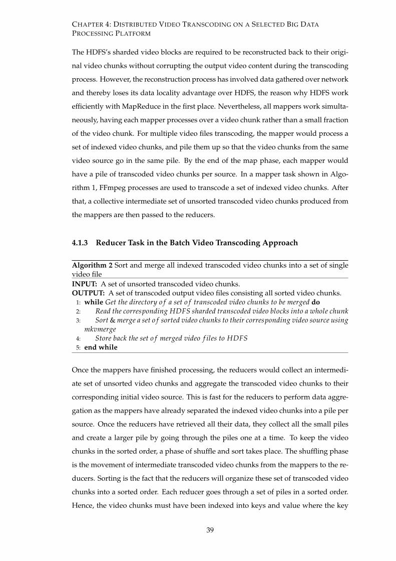
CHAPTER 4: DISTRIBUTED VIDEO TRANSCODING ON A SELECTED BIG DATA
PROCESSING PLATFORM
The HDFS’s sharded video blocks are required to be reconstructed back to their origi-
nal video chunks without corrupting the output video content during the transcoding
process. However, the reconstruction process has involved data gathered over network
and thereby loses its data locality advantage over HDFS, the reason why HDFS work
efficiently with MapReduce in the first place. Nevertheless, all mappers work simulta-
neously, having each mapper processes over a video chunk rather than a small fraction
of the video chunk. For multiple video files transcoding, the mapper would process a
set of indexed video chunks, and pile them up so that the video chunks from the same
video source go in the same pile. By the end of the map phase, each mapper would
have a pile of transcoded video chunks per source. In a mapper task shown in Algo-
rithm 1, FFmpeg processes are used to transcode a set of indexed video chunks. After
that, a collective intermediate set of unsorted transcoded video chunks produced from
the mappers are then passed to the reducers.
4.1.3 Reducer Task in the Batch Video Transcoding Approach
Algorithm 2 Sort and merge all indexed transcoded video chunks into a set of singlevideo fileINPUT: A set of unsorted transcoded video chunks.OUTPUT: A set of transcoded output video files consisting all sorted video chunks.
1: while Get the directory o f a set o f transcoded video chunks to be merged do2: Read the corresponding HDFS sharded transcoded video blocks into a whole chunk3: Sort & merge a set o f sorted video chunks to their corresponding video source using
mkvmerge4: Store back the set o f merged video f iles to HDFS5: end while
Once the mappers have finished processing, the reducers would collect an intermedi-
ate set of unsorted video chunks and aggregate the transcoded video chunks to their
corresponding initial video source. This is fast for the reducers to perform data aggre-
gation as the mappers have already separated the indexed video chunks into a pile per
source. Once the reducers have retrieved all their data, they collect all the small piles
and create a larger pile by going through the piles one at a time. To keep the video
chunks in the sorted order, a phase of shuffle and sort takes place. The shuffling phase
is the movement of intermediate transcoded video chunks from the mappers to the re-
ducers. Sorting is the fact that the reducers will organize these set of transcoded video
chunks into a sorted order. Each reducer goes through a set of piles in a sorted order.
Hence, the video chunks must have been indexed into keys and value where the key
39
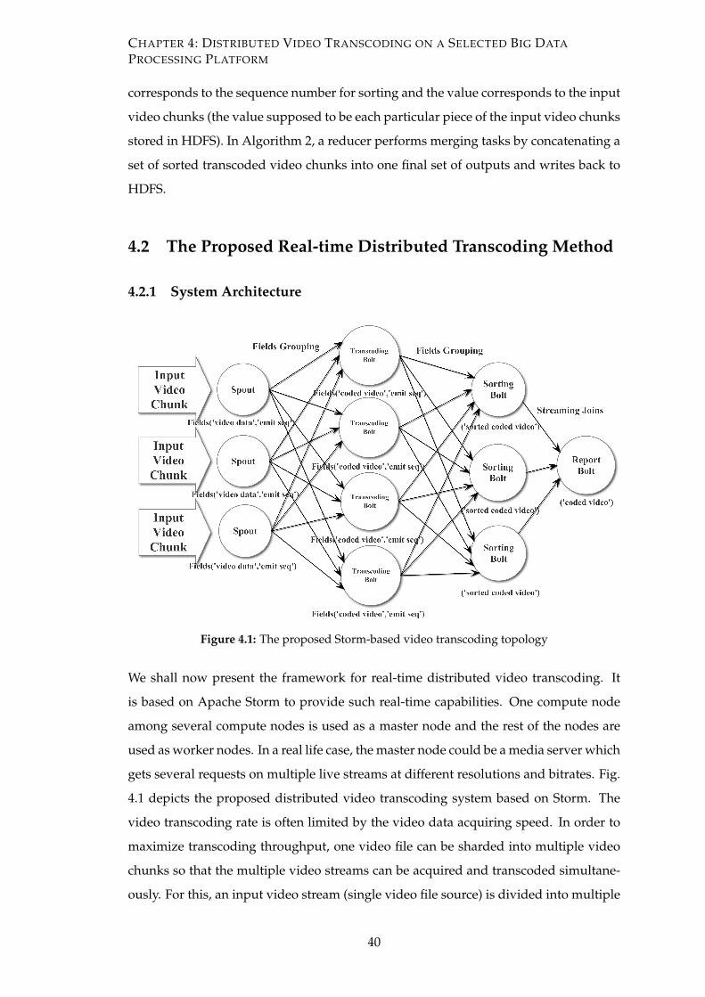
CHAPTER 4: DISTRIBUTED VIDEO TRANSCODING ON A SELECTED BIG DATA
PROCESSING PLATFORM
corresponds to the sequence number for sorting and the value corresponds to the input
video chunks (the value supposed to be each particular piece of the input video chunks
stored in HDFS). In Algorithm 2, a reducer performs merging tasks by concatenating a
set of sorted transcoded video chunks into one final set of outputs and writes back to
HDFS.
4.2 The Proposed Real-time Distributed Transcoding Method
4.2.1 System Architecture
Figure 4.1: The proposed Storm-based video transcoding topology
We shall now present the framework for real-time distributed video transcoding. It
is based on Apache Storm to provide such real-time capabilities. One compute node
among several compute nodes is used as a master node and the rest of the nodes are
used as worker nodes. In a real life case, the master node could be a media server which
gets several requests on multiple live streams at different resolutions and bitrates. Fig.
4.1 depicts the proposed distributed video transcoding system based on Storm. The
video transcoding rate is often limited by the video data acquiring speed. In order to
maximize transcoding throughput, one video file can be sharded into multiple video
chunks so that the multiple video streams can be acquired and transcoded simultane-
ously. For this, an input video stream (single video file source) is divided into multiple
40
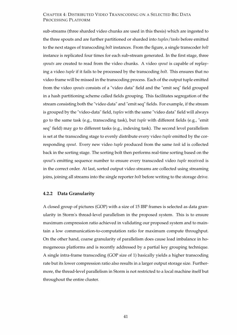
CHAPTER 4: DISTRIBUTED VIDEO TRANSCODING ON A SELECTED BIG DATA
PROCESSING PLATFORM
sub-streams (three sharded video chunks are used in this thesis) which are ingested to
the three spouts and are further partitioned or sharded into tuples/tasks before emitted
to the next stages of transcoding bolt instances. From the figure, a single transcoder bolt
instance is replicated four times for each sub-stream generated. In the first stage, three
spouts are created to read from the video chunks. A video spout is capable of replay-
ing a video tuple if it fails to be processed by the transcoding bolt. This ensures that no
video frame will be missed in the transcoding process. Each of the output tuple emitted
from the video spouts consists of a "video data" field and the "emit seq" field grouped
in a hash partitioning scheme called fields grouping. This facilitates segregation of the
stream consisting both the "video data" and "emit seq" fields. For example, if the stream
is grouped by the "video-data" field, tuples with the same "video data" field will always
go to the same task (e.g., transcoding task), but tuple with different fields (e.g., "emit
seq" field) may go to different tasks (e.g., indexing task). The second level parallelism
is set at the transcoding stage to evenly distribute every video tuple emitted by the cor-
responding spout. Every new video tuple produced from the same task id is collected
back in the sorting stage. The sorting bolt then performs real-time sorting based on the
spout's emitting sequence number to ensure every transcoded video tuple received is
in the correct order. At last, sorted output video streams are collected using streaming
joins, joining all streams into the single reporter bolt before writing to the storage drive.
4.2.2 Data Granularity
A closed group of pictures (GOP) with a size of 15 IBP frames is selected as data gran-
ularity in Storm's thread-level parallelism in the proposed system. This is to ensure
maximum compression ratio achieved in validating our proposed system and to main-
tain a low communication-to-computation ratio for maximum compute throughput.
On the other hand, coarse granularity of parallelism does cause load imbalance in ho-
mogeneous platforms and is recently addressed by a partial key grouping technique.
A single intra-frame transcoding (GOP size of 1) basically yields a higher transcoding
rate but its lower compression ratio also results in a larger output storage size. Further-
more, the thread-level parallelism in Storm is not restricted to a local machine itself but
throughout the entire cluster.
41
CHAPTER 4: DISTRIBUTED VIDEO TRANSCODING ON A SELECTED BIG DATA
PROCESSING PLATFORM
Figure 4.2: Processing data at a larger scale
4.2.3 Transcoding Videos at A Larger Scale
By referring to the experiment results of the proposed system in Table 5.10, the input
frame rate for Spout 1, 2 and 3 is 815 fps, 1568 fps and 1003 fps respectively. Transcoder
backends used in the experiment are capable of transcoding at 13 fps, 23 fps and 36 fps
when output resolution is set to 1080p. Therefore, the cluster takes 47 secs to transcode
1 sec of video frames. Meaning that by the end of 47 secs, 155756 frames are going to be
held in the data buffer and waiting to be processed. Since the cluster transcoding rate
is much lower than the total input frame rate, frames are keep on holding all way in the
queues. Thus, the system will never catch up with the input data rate and eventually
suffered from insufficient memory.
Fig. 4.2 shows how the stream processing system can handle the case where the input
frame rate is greater than the processing rate. In the previous example, our proposed
system acquires input videos at a total input video frame rate of 3386 frames per sec-
ond. To fully utilize such high input frame rate, Storm divides them into 47 small
buckets with each bucket transcoding a total of 72 frames per second. Basically, the op-
timized cluster size is equivalent to a cluster that is duplicated 47 times under the same
computers that the existing cluster is doing for one whole input stream acquiring at
3386 frames per second. This process is often refers to data sharding, where the entire
input stream is divided into multiple streams (e.g., 47 streams in our case) and running
the same transcoding program backend.
42
CHAPTER 4: DISTRIBUTED VIDEO TRANSCODING ON A SELECTED BIG DATA
PROCESSING PLATFORM
4.2.4 The Video Data Spout
The video data spout is the source of a storm-based video transcoder topology. At start-
up, it reads the GOP size, loads the video in exact GOP bytes sizes into main memory
and encode into base64 string characters before emitting them as Storm tuples. For the
input source of a camera stream, FFmpeg is used to read from the RTSP stream and the
video stream is converted to raw H.264 bit-streams. Similarly, the H.264 bit-streams are
then later encoded into base64 string characters before emitting to the transcoding bolt.
Algorithm 3 illustrates a reliable video data spout component. At initialization, the
video data is loaded into memory. Every time the nextTuple function is called, it will
emit a tuple in a list of GOPs in based64-encoded text, its emitting sequence and its
identification. Spout assigns every tuple with a global message identifier, which is later
used by a transcoding bolt to acknowledge (ack) the tuple. If the transcoding bolt fails
or the tuple experiences a timeout, the guaranteed message processing of Storm will
replay the tuple.
Algorithm 3 The GOP level of granularity for the input video spout method
INPUT: Input video frames.OUTPUT: A tuple grouped in a micro-batch list of 15 frames GOP, seqid and msgID.
1: function NEXTTUPLE() . The tuple to be emitted to the next consuming bolt2: msgID ← randomUUID3: while (bu f f er.size() < current computed GOP bytes size) do4: if nRead← input video stream read up to GOP byte size ! = empty then5: bu f f er ← nRead video bytes are concatenated to the previously stored bu f f er6: end if7: end while8: s← encode the bu f f er into base64 string characters9: seqid ++; . incrementing the emit sequence id for every tuple
10: The output collector emits tuple grouped in ((s, seqid), msgID)11: end function
4.2.5 The Transcoding Bolt
The transcoding bolt is the first stage of bolt instances found in the storm-based video
transcoder topology. In a bolt instance, the received tuple is decoded back to the video
bytes format and piped to the FFmpeg and FFprobe process respectively. The transcoded
output from the FFmpeg process is temporarily stored in key-value TreeMap. Fig. 4.3
illustrates the sample output data generated from the FFprobe process. FFprobe is used
to compute the GOP byte size for each video frame stored in TreeMap. Once the FFm-
43
CHAPTER 4: DISTRIBUTED VIDEO TRANSCODING ON A SELECTED BIG DATA
PROCESSING PLATFORM
peg process has completed the very last frame of a coded GOP, a single GOP packet
has been emitted to the reporter bolt in the final stage.
Algorithm 4 illustrates the algorithm of a transcoding bolt component. Similarly at
initialization, received tuples are loaded into memory. The tuple is then partitioned into
fields of "coded video" and "emit seq". The video source tuple received is converted
back to byte streams. Every time the next tuple is executed, a new output tuple in a
list of transcoded GOP in base64-coded text and its received sequence order will be
emitted. The bolt acknowledges (ack) the input tuple after it has successfully emitted
the transcoded GOP tuple. If the transcoding bolt fails or the input tuple experiences a
timeout, the guaranteed message processing of Storm will replay the tuple.
4.2.6 The Sorting Bolt
The sorting bolt is basically responsible for sorting the small piles of video tuples which
facilitates the final sort in the reporting bolt to create a larger pile from those small piles
stored in keys and value pair in terms of a sequence number and a set of video tuples
in accordance to their corresponding video source. This is done by using Treemap
where a set of video tuples are sorted in real time in a balanced binary search tree. This
sorting bolt can be neglected and needed only when there is way too many number
of transcoded video streams to be stored in memory for sorting purposes and which
could not handled by a reporting bolt alone.
4.2.7 The Reporting Bolt
Algorithm 5 shows a reporting bolt component. A reporting bolt is responsible for
gathering all transcoded GOP segments emitted from all worker nodes using streaming
joins. Every time the next tuple is received; the transcoded GOP is stored and sorted in
the correct order before writing them to the storage drive.
4.2.8 The Topology Builder
Algorithm 6 shows the spouts and bolts in building the topology and their parallelism
hint for thread-level parallelism. A spout emitted tuple consists of two fields, the GOP
and emitting sequence fields. The spout tuples are then distributed to the transcoding
bolts by fields grouping at parallelism of three. In the final stage, a reporter bolt gathers
44
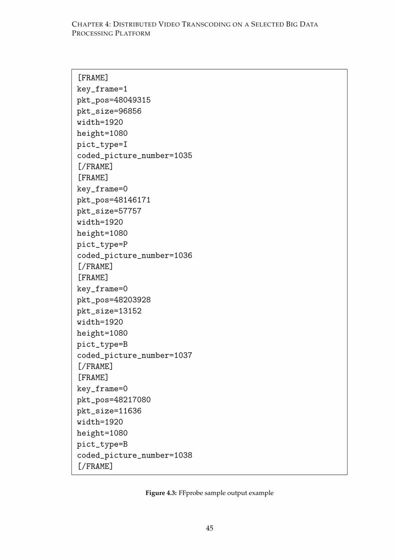
CHAPTER 4: DISTRIBUTED VIDEO TRANSCODING ON A SELECTED BIG DATA
PROCESSING PLATFORM
[FRAME]key_frame=1pkt_pos=48049315pkt_size=96856width=1920height=1080pict_type=Icoded_picture_number=1035[/FRAME][FRAME]key_frame=0pkt_pos=48146171pkt_size=57757width=1920height=1080pict_type=Pcoded_picture_number=1036[/FRAME][FRAME]key_frame=0pkt_pos=48203928pkt_size=13152width=1920height=1080pict_type=Bcoded_picture_number=1037[/FRAME][FRAME]key_frame=0pkt_pos=48217080pkt_size=11636width=1920height=1080pict_type=Bcoded_picture_number=1038[/FRAME]
Figure 4.3: FFprobe sample output example
45
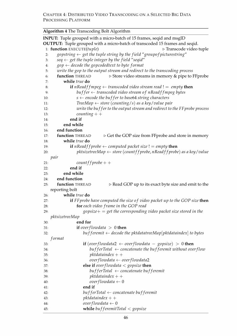
CHAPTER 4: DISTRIBUTED VIDEO TRANSCODING ON A SELECTED BIG DATA
PROCESSING PLATFORM
Algorithm 4 The Transcoding Bolt Algorithm
INPUT: Tuple grouped with a micro-batch of 15 frames, seqid and msgIDOUTPUT: Tuple grouped with a micro-batch of transcoded 15 frames and seqid.
1: function EXECUTE(tuple) . Transcode video tuple2: gopstring← get the tuple string by the f ield ”groupo f picturestring”3: seq← get the tuple integer by the f ield ”seqid”4: gop← decode the gopcodedtext to byte f ormat5: write the gop to the output stream and redirect to the transcoding process6: function THREAD . Store video streams in memory & pipe to FFprobe7: while true do8: if nRead f f mpeg← transcoded video stream read ! = empty then9: bu f f er ← transcoded video stream o f nRead f f mpeg bytes
10: s← encode the bu f f er to base64 string characters11: TreeMap← store (counting/s) as a key/value pair12: write the bu f f er to the output stream and redirect to the FFprobe process13: counting ++14: end if15: end while16: end function17: function THREAD . Get the GOP size from FFprobe and store in memory18: while true do19: if nRead f f probe← computed packet size ! = empty then20: pktsizetreeMap← store (count f f probe, nRead f f probe) as a key/value
pair21: count f f probe ++22: end if23: end while24: end function25: function THREAD . Read GOP up to its exact byte size and emit to the
reporting bolt26: while true do27: if FFprobe have computed the size o f video packet up to the GOP size then28: for each video f rame in the GOP read29: gopsize+ = get the corresponding video packet size stored in the
pktsizetreeMap30: end for31: if over f lowdata > 0 then32: bu f f eremit← decode the pktdatatreeMap[pktdataindex] to bytes
f ormat33: if (over f lowdata2 ← over f lowdata − gopsize) > 0 then34: bu f f erTotal ← concatenate the bu f f eremit without over f low35: pktdataindex ++36: over f lowdata← over f lowdata237: else if over f lowdata < gopsize then38: bu f f erTotal ← concatenate bu f f eremit39: pktdataindex ++40: over f lowdata← 041: end if42: bu f f erTotal ← concatenate bu f f eremit43: pktdataindex ++44: over f lowdata← 045: while bu f f eremitTotal < gopsize
46
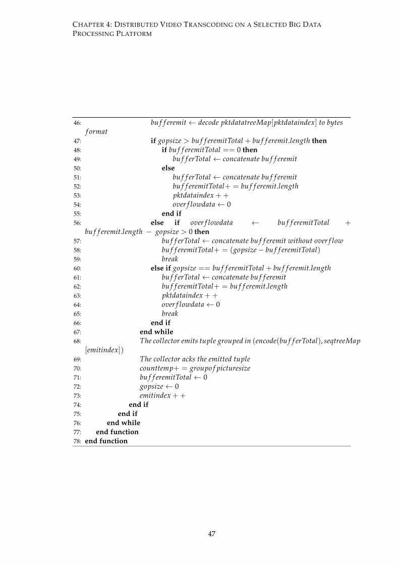
CHAPTER 4: DISTRIBUTED VIDEO TRANSCODING ON A SELECTED BIG DATA
PROCESSING PLATFORM
46: bu f f eremit← decode pktdatatreeMap[pktdataindex] to bytesf ormat
47: if gopsize > bu f f eremitTotal + bu f f eremit.length then48: if bu f f eremitTotal == 0 then49: bu f f erTotal ← concatenate bu f f eremit50: else51: bu f f erTotal ← concatenate bu f f eremit52: bu f f eremitTotal+ = bu f f eremit.length53: pktdataindex ++54: over f lowdata← 055: end if56: else if over f lowdata ← bu f f eremitTotal +
bu f f eremit.length − gopsize > 0 then57: bu f f erTotal ← concatenate bu f f eremit without over f low58: bu f f eremitTotal+ = (gopsize− bu f f eremitTotal)59: break60: else if gopsize == bu f f eremitTotal + bu f f eremit.length61: bu f f erTotal ← concatenate bu f f eremit62: bu f f eremitTotal+ = bu f f eremit.length63: pktdataindex ++64: over f lowdata← 065: break66: end if67: end while68: The collector emits tuple grouped in (encode(bu f f erTotal), seqtreeMap
[emitindex])69: The collector acks the emitted tuple70: counttemp+ = groupo f picturesize71: bu f f eremitTotal ← 072: gopsize← 073: emitindex ++74: end if75: end if76: end while77: end function78: end function
47
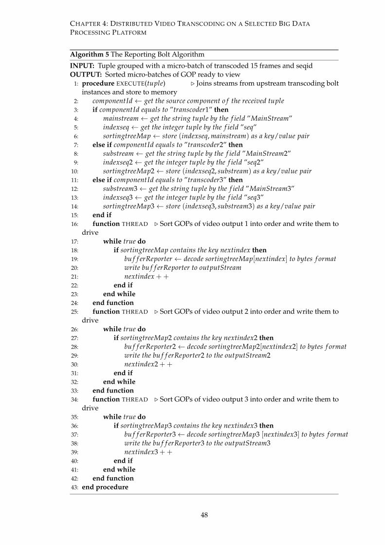
CHAPTER 4: DISTRIBUTED VIDEO TRANSCODING ON A SELECTED BIG DATA
PROCESSING PLATFORM
Algorithm 5 The Reporting Bolt Algorithm
INPUT: Tuple grouped with a micro-batch of transcoded 15 frames and seqidOUTPUT: Sorted micro-batches of GOP ready to view
1: procedure EXECUTE(tuple) . Joins streams from upstream transcoding boltinstances and store to memory
2: componentId← get the source component o f the received tuple3: if componentId equals to ”transcoder1” then4: mainstream← get the string tuple by the f ield ”MainStream”5: indexseq← get the integer tuple by the f ield ”seq”6: sortingtreeMap← store (indexseq, mainstream) as a key/value pair7: else if componentId equals to ”transcoder2” then8: substream← get the string tuple by the f ield ”MainStream2”9: indexseq2← get the integer tuple by the f ield ”seq2”
10: sortingtreeMap2← store (indexseq2, substream) as a key/value pair11: else if componentId equals to ”transcoder3” then12: substream3← get the string tuple by the f ield ”MainStream3”13: indexseq3← get the integer tuple by the f ield ”seq3”14: sortingtreeMap3← store (indexseq3, substream3) as a key/value pair15: end if16: function THREAD . Sort GOPs of video output 1 into order and write them to
drive17: while true do18: if sortingtreeMap contains the key nextindex then19: bu f f erReporter ← decode sortingtreeMap[nextindex] to bytes f ormat20: write bu f f erReporter to outputStream21: nextindex ++22: end if23: end while24: end function25: function THREAD . Sort GOPs of video output 2 into order and write them to
drive26: while true do27: if sortingtreeMap2 contains the key nextindex2 then28: bu f f erReporter2← decode sortingtreeMap2[nextindex2] to bytes f ormat29: write the bu f f erReporter2 to the outputStream230: nextindex2 ++31: end if32: end while33: end function34: function THREAD . Sort GOPs of video output 3 into order and write them to
drive35: while true do36: if sortingtreeMap3 contains the key nextindex3 then37: bu f f erReporter3← decode sortingtreeMap3 [nextindex3] to bytes f ormat38: write the bu f f erReporter3 to the outputStream339: nextindex3 ++40: end if41: end while42: end function43: end procedure
48

CHAPTER 4: DISTRIBUTED VIDEO TRANSCODING ON A SELECTED BIG DATA
PROCESSING PLATFORM
all transcoded GOPs by joining tuples to one point. Again, each tuple is grouped by
fields grouping.
4.2.9 The Storm Pluggable Scheduler
In Storm, Nimbus uses a scheduler to assign executors to supervisors. The default sched-
uler of Storm aims at scheduling computing resources evenly to the topology compo-
nents (spouts and bolts). In a homogenous Storm cluster, the default scheduler works
well in terms of fairness distribution among topology components but it is unpre-
dictable for users to locate the placement of every topology component in the Storm
cluster. In a heterogeneous platform such as one used in our proposed system, we
have faced unfair scheduling in the storm default scheduler where more executors are
assigned to a supervisor results in executing more tasks and underloading on the other
side. Therefore, we have implemented a custom scheduler to address this issue. On the
other hand, users can reserve the name of supervisors under storm.scheduler.meta in a
configuration file, in which users can specify any supervisors in a "key-value" pairs to
facilitate task scheduling. For instance, the scheduler ensures that a spout named "Main-
Spout" in the topology "video topology" runs on a supervisor named "supervisor1" can
be configured at supervisor.scheduler.meta. If a Storm’s component consists of three
executors, the scheduler will allocate three workers from three different selected super-
visors to the executors accordingly. The number of executors for a Storm’s component
is basically corresponding to the number of parallelism hint set in stream groupings.
Algorithm 7 shows the portion of the scheduler code for video spouts. First, we find
out all components and executors of the topology that are needed for scheduling. Next,
component’s executors are scheduled to specified supervisors for task execution. Similar
method is applied to the transcoding bolt instances and the reporter bolt instance in the
proposed system.
4.2.10 Storm Custom Stream Grouping
There are many stream groupings provided in Storm. These groupings are respon-
sible for the task assignment in which the emitted tuples are sent to the consuming
bolt instances. A key or fields grouping is a strategy used in the stream processing
framework to simplify the development of parallel stateful operators. Inside the fields
grouping approach, a stream of tuples is usually partitioned based on the key of the
49
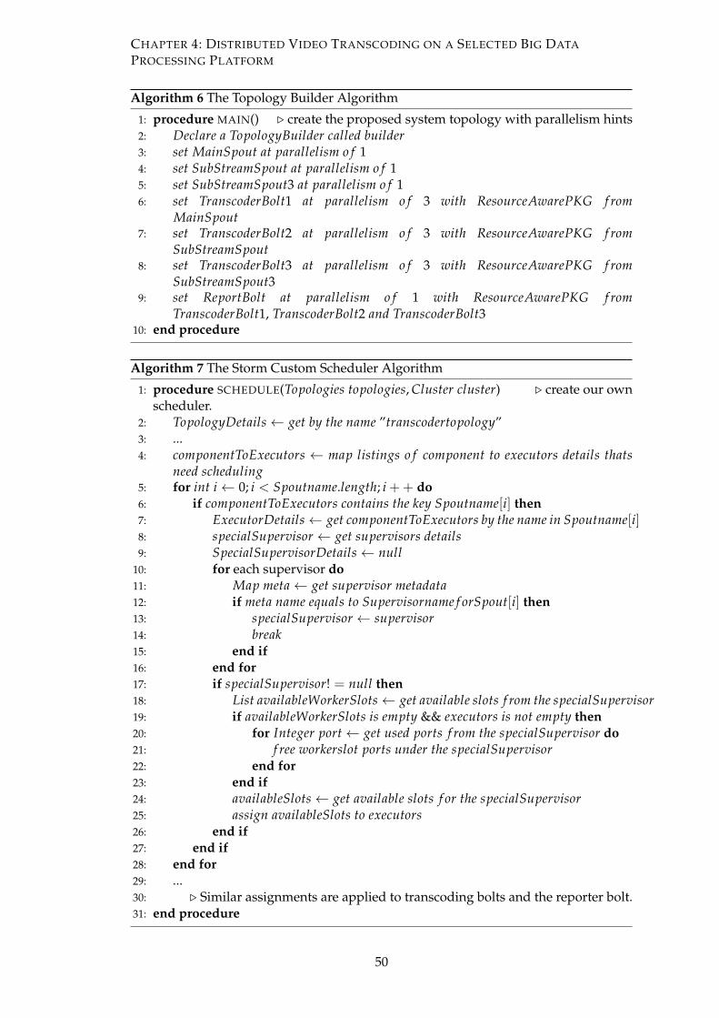
CHAPTER 4: DISTRIBUTED VIDEO TRANSCODING ON A SELECTED BIG DATA
PROCESSING PLATFORM
Algorithm 6 The Topology Builder Algorithm
1: procedure MAIN() . create the proposed system topology with parallelism hints2: Declare a TopologyBuilder called builder3: set MainSpout at parallelism o f 14: set SubStreamSpout at parallelism o f 15: set SubStreamSpout3 at parallelism o f 16: set TranscoderBolt1 at parallelism o f 3 with ResourceAwarePKG f rom
MainSpout7: set TranscoderBolt2 at parallelism o f 3 with ResourceAwarePKG f rom
SubStreamSpout8: set TranscoderBolt3 at parallelism o f 3 with ResourceAwarePKG f rom
SubStreamSpout39: set ReportBolt at parallelism o f 1 with ResourceAwarePKG f rom
TranscoderBolt1, TranscoderBolt2 and TranscoderBolt310: end procedure
Algorithm 7 The Storm Custom Scheduler Algorithm
1: procedure SCHEDULE(Topologies topologies, Cluster cluster) . create our ownscheduler.
2: TopologyDetails← get by the name ”transcodertopology”3: ...4: componentToExecutors ← map listings o f component to executors details thats
need scheduling5: for int i← 0; i < Spoutname.length; i ++ do6: if componentToExecutors contains the key Spoutname[i] then7: ExecutorDetails← get componentToExecutors by the name in Spoutname[i]8: specialSupervisor ← get supervisors details9: SpecialSupervisorDetails← null
10: for each supervisor do11: Map meta← get supervisor metadata12: if meta name equals to Supervisorname f orSpout[i] then13: specialSupervisor ← supervisor14: break15: end if16: end for17: if specialSupervisor! = null then18: List availableWorkerSlots← get available slots f rom the specialSupervisor19: if availableWorkerSlots is empty && executors is not empty then20: for Integer port← get used ports f rom the specialSupervisor do21: f ree workerslot ports under the specialSupervisor22: end for23: end if24: availableSlots← get available slots f or the specialSupervisor25: assign availableSlots to executors26: end if27: end if28: end for29: ...30: . Similar assignments are applied to transcoding bolts and the reporter bolt.31: end procedure
50
CHAPTER 4: DISTRIBUTED VIDEO TRANSCODING ON A SELECTED BIG DATA
PROCESSING PLATFORM
stream into several disjoint sub-streams, ensuring tuples with the same key are pro-
cessed by the workers of the same bolt. Typically, a hash function is used to map the
tuple key to its corresponding sub-stream. Such hash-based routing allows sub-stream
messages to be routed from their sources solely via their key, without needing to keep
any state or to coordinate among bolts. Fields grouping is also known as a "single-
choice" paradigm which causes imbalance in task distribution across the Storm clus-
ter since it disregards the frequency of messages with the same key appearing during
stream grouping. Hence, fields grouping basically groups data based on hash assign-
ment which is scalable, has low memory but is stateful and load imbalance. In order to
achieve excellent load balancing, another partitioning scheme called shuffle grouping
is used. This is done in a round-robin routing approach which sends messages to a
bolt in cyclic order, irrespective of their keys. However, this scheme is mostly used for
stateless computation. An additional aggregation phase and memory are required for
computation, and grouped by shuffle grouping to become stateful. Nasir, Muhammad
Anis Uddin, et al. [111] introduced Partial Key Grouping (PKG), a new stream parti-
tioning scheme that achieves better load balancing than fields grouping while incurring
less overhead memory compared to shuffle grouping. Authors in [111] focus on solv-
ing issues of load balancing on stateful applications when key distribution is skewed
(limited scalability). In PKG, the upstream spout creates a balanced partition of mes-
sages for the downstream bolts, attaining load balancing for each edge of DAG. They
claimed that by comparing it to fields grouping, PKG reduces load imbalance to multi-
ple orders of magnitude. Thus, the throughput and latency of an example application
can be improved by up to 45%.
4.2.11 The Resource-Aware Task Allocation Scheme
In a homogeneous computing environment, every node has identical performance and
capacity. Effective task scheduling is measured by the quantity of nodes instead of their
individual quality since the resources are allocated evenly across all available nodes.
For most cases, task scheduling and resource allocation in the homogeneous comput-
ing environment divide workload across all nodes evenly, which results in identical
workload distribution across all nodes. Contrary to the homogeneous computing en-
vironment, computing nodes have different computing performances and capacities
in heterogeneous systems. Under identical workload distribution, high-performance
nodes can process data faster than the low-performance nodes. This session proposes
51
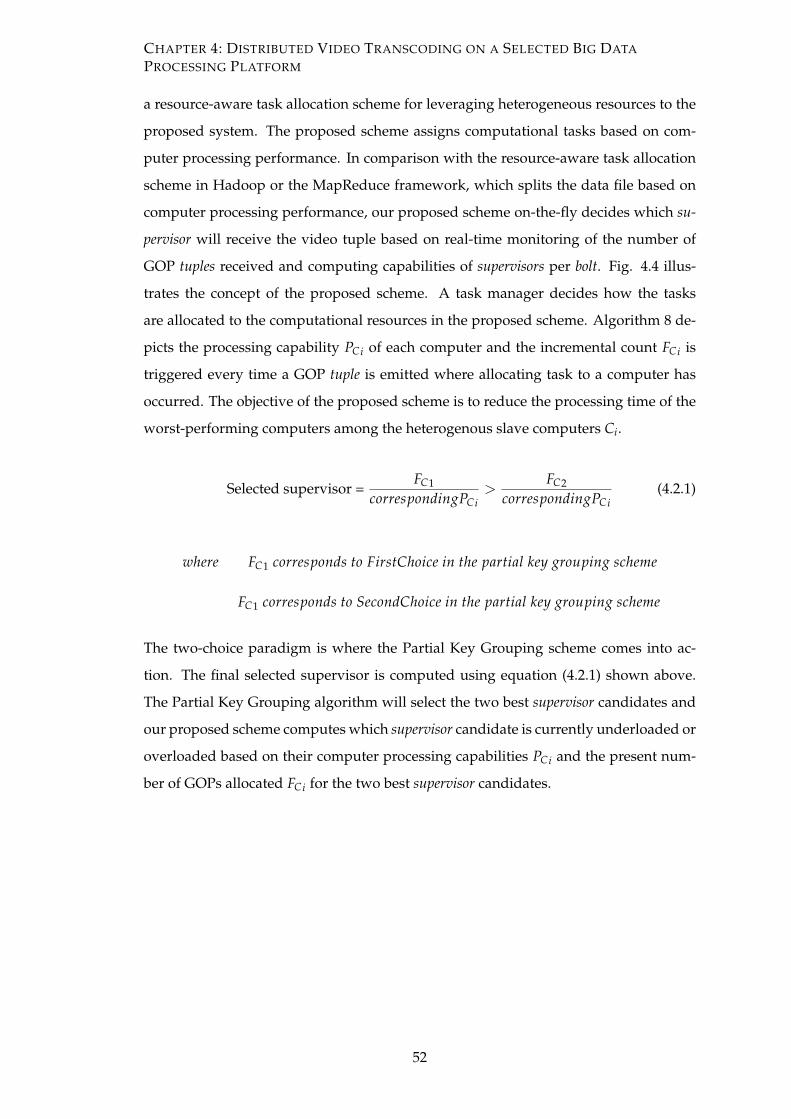
CHAPTER 4: DISTRIBUTED VIDEO TRANSCODING ON A SELECTED BIG DATA
PROCESSING PLATFORM
a resource-aware task allocation scheme for leveraging heterogeneous resources to the
proposed system. The proposed scheme assigns computational tasks based on com-
puter processing performance. In comparison with the resource-aware task allocation
scheme in Hadoop or the MapReduce framework, which splits the data file based on
computer processing performance, our proposed scheme on-the-fly decides which su-
pervisor will receive the video tuple based on real-time monitoring of the number of
GOP tuples received and computing capabilities of supervisors per bolt. Fig. 4.4 illus-
trates the concept of the proposed scheme. A task manager decides how the tasks
are allocated to the computational resources in the proposed scheme. Algorithm 8 de-
picts the processing capability PCi of each computer and the incremental count FCi is
triggered every time a GOP tuple is emitted where allocating task to a computer has
occurred. The objective of the proposed scheme is to reduce the processing time of the
worst-performing computers among the heterogenous slave computers Ci.
Selected supervisor =FC1
correspondingPCi>
FC2
correspondingPCi(4.2.1)
where FC1 corresponds to FirstChoice in the partial key grouping scheme
FC1 corresponds to SecondChoice in the partial key grouping scheme
The two-choice paradigm is where the Partial Key Grouping scheme comes into ac-
tion. The final selected supervisor is computed using equation (4.2.1) shown above.
The Partial Key Grouping algorithm will select the two best supervisor candidates and
our proposed scheme computes which supervisor candidate is currently underloaded or
overloaded based on their computer processing capabilities PCi and the present num-
ber of GOPs allocated FCi for the two best supervisor candidates.
52
CHAPTER 4: DISTRIBUTED VIDEO TRANSCODING ON A SELECTED BIG DATA
PROCESSING PLATFORM
Algorithm 8 The Resource-Aware Stream Grouping Algorithm
1: procedure PREPARE(WorkerTopologyContext, GlobalStreamId & a list o f targetTasks)2: this.targetTasks← targetTasks;3: if GlobalStreamId. f ields! = null then4: GlobalStreamId.outFields← get component output f ields f or the stream5: end if6: declare an integer array named assignedtuples with the size o f targetTasks.size()7: end procedure8: procedure CHOOSETASKS(int taskId, List o f values)9: List o f integer boltIds← ArrayList[1]
10: if values.size() > 0 then11: { i.e.Partial Key Grouping Algorithms . Any Grouping Algorithm12: ...13: f irstChoice← Math.abs(h1.hashBytes(raw).asLong())%targetTasks.size()14: secondChoice← Math.abs(h2.hashBytes(raw).asLong())%targetTasks.size()15: }16: switch f irstChoice do17: case 018: assert(b1← PC0)19: case 120: assert(b1← PC1)21: case 222: assert(b1← PC2)23: switch secondChoice do24: case 025: assert(b2← PC0)26: case 127: assert(b2← PC1)28: case 229: assert(b2← PC2)30: selected ← i f (assignedtuples[ f irstChoice] ∗ 15/b1) >
(assignedtuples[secondChoice] ∗ 15/b2) then choose secondChoice else choosef irstChoice . resource-aware task allocation, refer to equation (4.2.1)
31: boltIds add targetTasks.get(selected)32: assignedtuples[selected] + +;33: end if34: return boltIds;35: end procedure
53
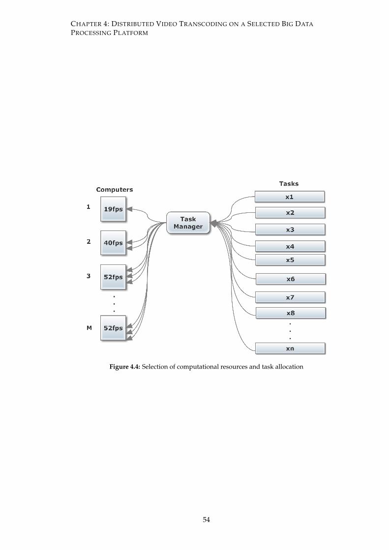
CHAPTER 4: DISTRIBUTED VIDEO TRANSCODING ON A SELECTED BIG DATA
PROCESSING PLATFORM
Figure 4.4: Selection of computational resources and task allocation
54
CHAPTER 5
Experimental Results and
Discussions
The proposed framework in Section 4.2 is implemented in this chapter. The first few
sections investigate the performance evaluation on some existing researches that have
been previously done on this area, comparing with the proposed system. The remain-
ing of this chapter validates our proposed system in terms of data granularity and fair
resource-aware task allocation to heterogenous systems. Finally, the produced output
videos are rated to ensure meeting the expected quality standard.
5.1 Performance Evaluation
Four computers with their CPU and GPU specifications listed in Table 5.1 were used in
the experiment. GPUs were used as a related work comparison to the proposed system.
A test sequence (Big Buck Bunny, 1920×1080, 24 fps, 9 minutes 57 seconds) was used to
simulate a real-time video stream and was transcoded into the H.264 format with mul-
tiple output resolutions (1920×1080 or 1080p, 1280×720 or 720p and 640×480 or 480p)
using the proposed real-time distributed system to obtain the maximum capability of
the system.
5.1.1 The Nvidia Hardware Encoder
Table 5.2 presents the average transcoding rate of the related work, NVENC when dif-
ferent output resolutions are selected. The input video stream is divided into multiple
sub-streams, allowing multiple transcoding instances to be executed simultaneously.
55
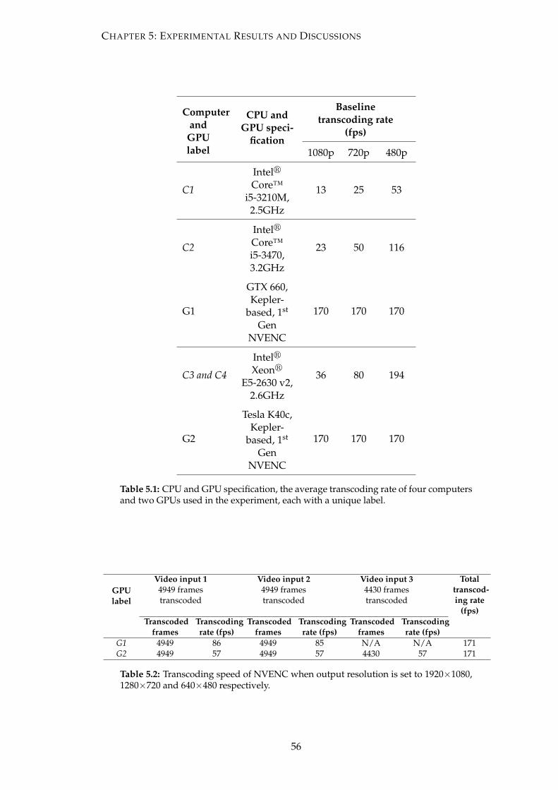
CHAPTER 5: EXPERIMENTAL RESULTS AND DISCUSSIONS
ComputerandGPUlabel
CPU andGPU speci-
fication
Baselinetranscoding rate
(fps)
1080p 720p 480p
C1
Intelr
Core™i5-3210M,2.5GHz
13 25 53
C2
Intelr
Core™i5-3470,3.2GHz
23 50 116
G1
GTX 660,Kepler-
based, 1st
GenNVENC
170 170 170
C3 and C4
Intelr
Xeonr
E5-2630 v2,2.6GHz
36 80 194
G2
Tesla K40c,Kepler-
based, 1st
GenNVENC
170 170 170
Table 5.1: CPU and GPU specification, the average transcoding rate of four computersand two GPUs used in the experiment, each with a unique label.
GPUlabel
Video input 1 Video input 2 Video input 3 Totaltranscod-ing rate
(fps)
4949 framestranscoded
4949 framestranscoded
4430 framestranscoded
Transcodedframes
Transcodingrate (fps)
Transcodedframes
Transcodingrate (fps)
Transcodedframes
Transcodingrate (fps)
G1 4949 86 4949 85 N/A N/A 171G2 4949 57 4949 57 4430 57 171
Table 5.2: Transcoding speed of NVENC when output resolution is set to 1920×1080,1280×720 and 640×480 respectively.
56
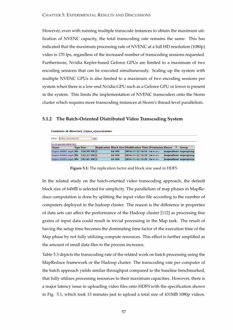
CHAPTER 5: EXPERIMENTAL RESULTS AND DISCUSSIONS
However, even with running multiple transcode instances to obtain the maximum uti-
lization of NVENC capacity, the total transcoding rate remains the same. This has
indicated that the maximum processing rate of NVENC at a full HD resolution (1080p)
video is 170 fps, regardless of the increased number of transcoding sessions requested.
Furthermore, Nvidia Kepler-based Geforce GPUs are limited to a maximum of two
encoding sessions that can be executed simultaneously. Scaling up the system with
multiple NVENC GPUs is also limited to a maximum of two encoding sessions per
system when there is a low-end Nvidia GPU such as a Geforce GPU or lower is present
in the system. This limits the implementation of NVENC transcoders onto the Storm
cluster which requires more transcoding instances at Storm's thread-level parallelism.
5.1.2 The Batch-Oriented Distributed Video Transcoding System
Figure 5.1: The replication factor and block size used in HDFS
In the related study on the batch-oriented video transcoding approach, the default
block size of 64MB is selected for simplicity. The parallelism of map phases in MapRe-
duce computation is done by splitting the input video file according to the number of
computers deployed in the hadoop cluster. The reason is the difference in properties
of data sets can affect the performance of the Hadoop cluster [112] as processing fine
grains of input data could result in trivial processing in the Map task. The result of
having the setup time becomes the dominating time factor of the execution time of the
Map phase by not fully utilizing compute resources. This effect is further amplified as
the amount of small data files to the process increases.
Table 5.3 depicts the transcoding rate of the related work on batch processing using the
MapReduce framework or the Hadoop cluster. The transcoding rate per computer of
the batch approach yields similar throughput compared to the baseline benchmarked,
that fully utilizes processing resources to their maximum capacities. However, there is
a major latency issue in uploading video files onto HDFS with the specification shown
in Fig. 5.1, which took 13 minutes just to upload a total size of 431MB 1080p videos.
57
CHAPTER 5: EXPERIMENTAL RESULTS AND DISCUSSIONS
Once the video transcoding batch job begins, the batch job continues until it is done.
There is no interaction with the user while the transcoding process is being executed.
The user has to wait until the job finishes since the transcoded video frames are un-
reachable during video transcoding as the output video frames are stored locally on
other compute nodes. Uploading output video files back to HDFS only begins when
the transcoded video chunks have been completely written to local temporary stor-
ages. Furthermore, the input video file is not sharded into size according to computing
ratios in this related study experiment, leaving poor load distribution in the hadoop
heterogeneous computing platform.
58
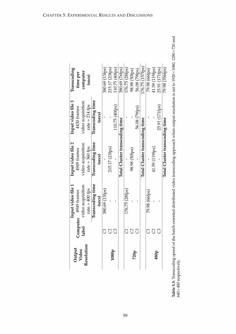
CHAPTER 5: EXPERIMENTAL RESULTS AND DISCUSSIONS
Out
put
Vid
eoR
esol
utio
n
Com
pute
rla
bel
Inpu
tvid
eofil
e1
Inpu
tvid
eofil
e2
Inpu
tvid
eofil
e3
Tran
scod
ing
tim
epe
rco
mpu
ter
(sec
s)
4949
fram
es49
49fr
ames
4430
fram
esvi
deo
acqu
isit
ion
rate
=40
0fp
svi
deo
acqu
isit
ion
rate
=36
0fp
svi
deo
acqu
isit
ion
rate
=21
4fp
sTr
ansc
odin
gti
me
(sec
s)Tr
ansc
odin
gti
me
(sec
s)Tr
ansc
odin
gti
me
(sec
s)
1080
p
C1
380.
69(1
3fps
)-
-38
0.69
(13f
ps)
C2
-21
5.17
(23f
ps)
-21
5.17
(23f
ps)
C3
--
110.
75(4
0fps
)11
0.75
(40f
ps)
Tota
lClu
ster
tran
scod
ing
tim
e38
0.69
(76f
ps)
720p
C1
176.
75(2
8fps
)-
-17
6.75
(28f
ps)
C2
-98
.98
(50f
ps)
-98
.98
(50f
ps)
C3
--
56.0
8(7
9fps
)56
.08
(79f
ps)
Tota
lClu
ster
tran
scod
ing
tim
e17
6.75
(157
fps)
480p
C1
79.9
8(6
6fps
)-
-79
.98
(66f
ps)
C2
-41
.59
(119
fps)
-41
.59
(119
fps)
C3
--
25.9
1(1
71fp
s)25
.91
(171
fps)
Tota
lClu
ster
tran
scod
ing
tim
e79
.98
(356
fps)
Tabl
e5.
3:Tr
ansc
odin
gsp
eed
ofth
eba
tch-
orie
nted
dist
ribu
ted
vide
otr
ansc
odin
gap
proa
chw
hen
outp
utre
solu
tion
isse
tto
1920×
1080
,128
0×72
0an
d64
0×48
0re
spec
tive
ly.
59
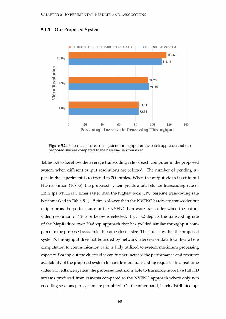
CHAPTER 5: EXPERIMENTAL RESULTS AND DISCUSSIONS
5.1.3 Our Proposed System
83.51
96.25
111.11
83.51
94.75
116.67
0 20 40 60 80 100 120 140
480p
720p
1080p
Percentage Increase in Processing Throughput
Vid
eo R
esol
utio
nTHE BATCH DISTRIBUTED VIDEO TRANSCODER THE PROPOSED SYSTEM
Figure 5.2: Percentage increase in system throughput of the batch approach and ourproposed system compared to the baseline benchmarked
Tables 5.4 to 5.6 show the average transcoding rate of each computer in the proposed
system when different output resolutions are selected. The number of pending tu-
ples in the experiment is restricted to 200 tuples. When the output video is set to full
HD resolution (1080p), the proposed system yields a total cluster transcoding rate of
115.2 fps which is 3 times faster than the highest local CPU baseline transcoding rate
benchmarked in Table 5.1, 1.5 times slower than the NVENC hardware transcoder but
outperforms the performance of the NVENC hardware transcoder when the output
video resolution of 720p or below is selected. Fig. 5.2 depicts the transcoding rate
of the MapReduce over Hadoop approach that has yielded similar throughput com-
pared to the proposed system in the same cluster size. This indicates that the proposed
system’s throughput does not bounded by network latencies or data localities where
computation to communication ratio is fully utilized to system maximum processing
capacity. Scaling out the cluster size can further increase the performance and resource
availability of the proposed system to handle more transcoding requests. In a real-time
video surveillance system, the proposed method is able to transcode more live full HD
streams produced from cameras compared to the NVENC approach where only two
encoding sessions per system are permitted. On the other hand, batch distributed ap-
60
CHAPTER 5: EXPERIMENTAL RESULTS AND DISCUSSIONS
proaches cannot to be implemented on real-time transcoding of live video streams since
they only consume data via files. Additionally, a full HD resolution video stream re-
quest is normally delivered using the original video source without transcoding. Thus,
the high transcoding rate at lower resolutions in the proposed system is more demand-
ing than the NVENC approach.
5.1.4 Load Distribution in the Proposed System
From Tables 5.4 to 5.6, one can see that the number of frames transcoded for all comput-
ers is similar to each other. The Storm’s task allocation scheme distributes video frames
across the cluster evenly. This is due to the fact that stream groupings used in Storm
apply a simple round-robin algorithm that does not consider heterogeneous processing
rates, leaving poor load distribution in the heterogeneous video transcoding platform.
Therefore, the performance of the entire system is bounded by the worst-performing
computer in the system. This issue has been addressed in sections 5.3 and 5.4 by ap-
plying the resource-aware task allocation scheme proposed in section 4.2.11.
61
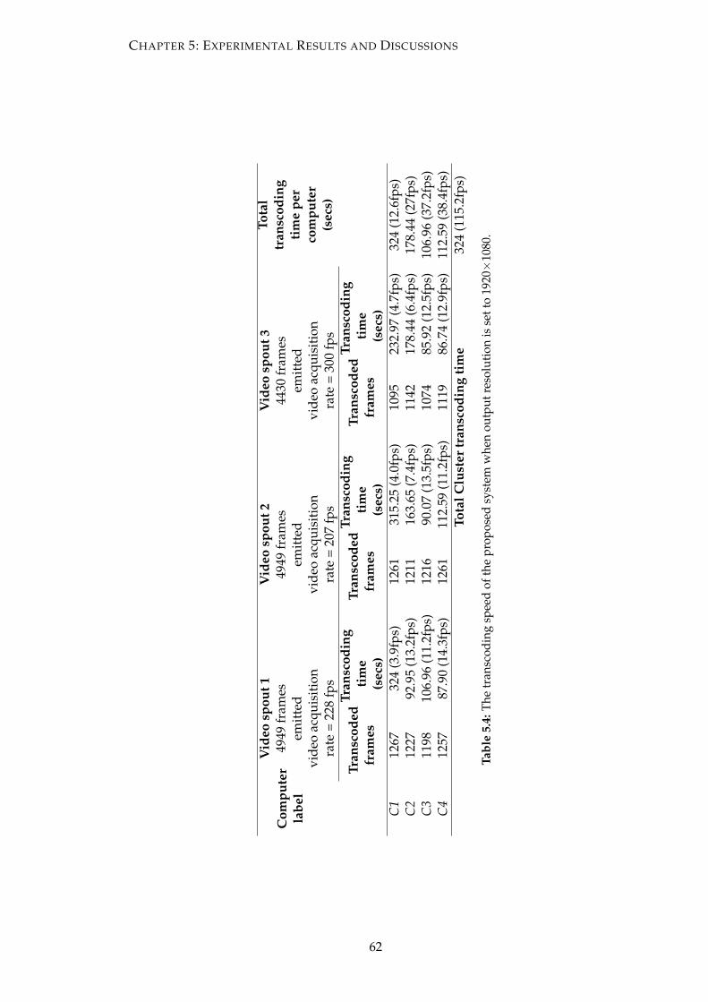
CHAPTER 5: EXPERIMENTAL RESULTS AND DISCUSSIONS
Com
pute
rla
bel
Vid
eosp
out 1
Vid
eosp
out2
Vid
eosp
out3
Tota
ltr
ansc
odin
gti
me
per
com
pute
r(s
ecs)
4949
fram
esem
itte
d49
49fr
ames
emit
ted
4430
fram
esem
itte
dvi
deo
acqu
isit
ion
rate
=22
8fp
svi
deo
acqu
isit
ion
rate
=20
7fp
svi
deo
acqu
isit
ion
rate
=30
0fp
s
Tran
scod
edfr
ames
Tran
scod
ing
tim
e(s
ecs)
Tran
scod
edfr
ames
Tran
scod
ing
tim
e(s
ecs)
Tran
scod
edfr
ames
Tran
scod
ing
tim
e(s
ecs)
C1
1267
324
(3.9
fps)
1261
315.
25(4
.0fp
s)10
9523
2.97
(4.7
fps)
324
(12.
6fps
)C
212
2792
.95
(13.
2fps
)12
1116
3.65
(7.4
fps)
1142
178.
44(6
.4fp
s)17
8.44
(27f
ps)
C3
1198
106.
96(1
1.2f
ps)
1216
90.0
7(1
3.5f
ps)
1074
85.9
2(1
2.5f
ps)
106.
96(3
7.2f
ps)
C4
1257
87.9
0(1
4.3f
ps)
1261
112.
59(1
1.2f
ps)
1119
86.7
4(1
2.9f
ps)
112.
59(3
8.4f
ps)
Tota
lClu
ster
tran
scod
ing
tim
e32
4(1
15.2
fps)
Tabl
e5.
4:Th
etr
ansc
odin
gsp
eed
ofth
epr
opos
edsy
stem
whe
nou
tput
reso
luti
onis
sett
o19
20×
1080
.
62
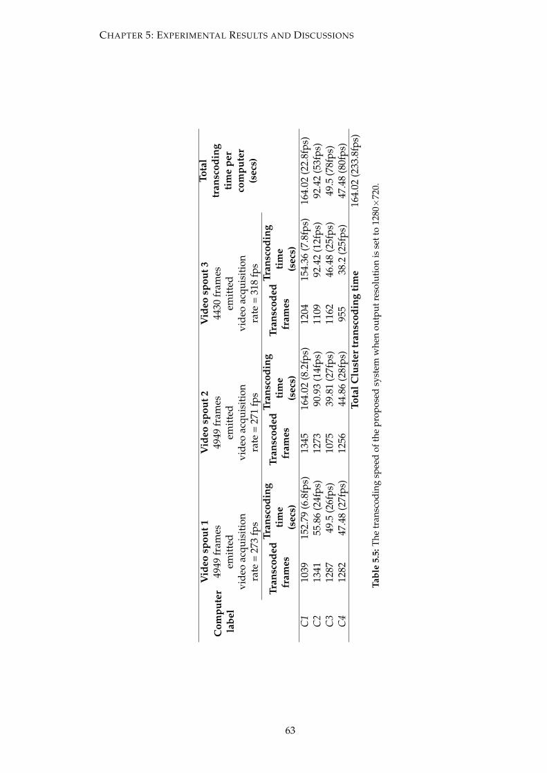
CHAPTER 5: EXPERIMENTAL RESULTS AND DISCUSSIONS
Com
pute
rla
bel
Vid
eosp
out 1
Vid
eosp
out2
Vid
eosp
out3
Tota
ltr
ansc
odin
gti
me
per
com
pute
r(s
ecs)
4949
fram
esem
itte
d49
49fr
ames
emit
ted
4430
fram
esem
itte
dvi
deo
acqu
isit
ion
rate
=27
3fp
svi
deo
acqu
isit
ion
rate
=27
1fp
svi
deo
acqu
isit
ion
rate
=31
8fp
s
Tran
scod
edfr
ames
Tran
scod
ing
tim
e(s
ecs)
Tran
scod
edfr
ames
Tran
scod
ing
tim
e(s
ecs)
Tran
scod
edfr
ames
Tran
scod
ing
tim
e(s
ecs)
C1
1039
152.
79(6
.8fp
s)13
4516
4.02
(8.2
fps)
1204
154.
36(7
.8fp
s)16
4.02
(22.
8fps
)C
213
4155
.86
(24f
ps)
1273
90.9
3(1
4fps
)11
0992
.42
(12f
ps)
92.4
2(5
3fps
)C
312
8749
.5(2
6fps
)10
7539
.81
(27f
ps)
1162
46.4
8(2
5fps
)49
.5(7
8fps
)C
412
8247
.48
(27f
ps)
1256
44.8
6(2
8fps
)95
538
.2(2
5fps
)47
.48
(80f
ps)
Tota
lClu
ster
tran
scod
ing
tim
e16
4.02
(233
.8fp
s)
Tabl
e5.
5:Th
etr
ansc
odin
gsp
eed
ofth
epr
opos
edsy
stem
whe
nou
tput
reso
luti
onis
sett
o12
80×
720.
63
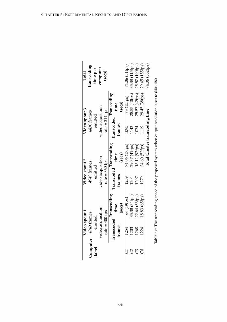
CHAPTER 5: EXPERIMENTAL RESULTS AND DISCUSSIONS
Com
pute
rla
bel
Vid
eosp
out 1
Vid
eosp
out2
Vid
eosp
out3
Tota
ltr
ansc
odin
gti
me
per
com
pute
r(s
ecs)
4949
fram
esem
itte
d49
49fr
ames
emit
ted
4430
fram
esem
itte
dvi
deo
acqu
isit
ion
rate
=40
0fp
svi
deo
acqu
isit
ion
rate
=36
0fp
svi
deo
acqu
isit
ion
rate
=21
4fp
s
Tran
scod
edfr
ames
Tran
scod
ing
tim
e(s
ecs)
Tran
scod
edfr
ames
Tran
scod
ing
tim
e(s
ecs)
Tran
scod
edfr
ames
Tran
scod
ing
tim
e(s
ecs)
C1
1254
66(1
9fps
)12
5974
.06
(17f
ps)
1095
73(1
5fps
)74
.06
(51f
ps)
C2
1203
35.3
8(3
4fps
)12
0429
.37
(41f
ps)
1142
28.5
5(4
0fps
)35
.38
(115
fps)
C3
1268
22.6
4(5
6fps
)12
0713
.12
(92f
ps)
1074
25.5
7(4
2fps
)25
.57
(190
fps)
C4
1224
18.8
3(6
5fps
)12
7924
.60
(52f
ps)
1119
29.4
5(3
8fps
)29
.45
(155
fps)
Tota
lClu
ster
tran
scod
ing
tim
e74
.06
(552
fps)
Tabl
e5.
6:Th
etr
ansc
odin
gsp
eed
ofth
epr
opos
edsy
stem
whe
nou
tput
reso
luti
onis
sett
o64
0×48
0.
64
CHAPTER 5: EXPERIMENTAL RESULTS AND DISCUSSIONS
5.2 Comparative Evaluation of the Fine- and Coarse-Grain Ap-
proach for the Proposed System
One of the important aspects in designing the architecture of our proposed system is
the issue of data granularity. This experiment is run on different granularity sizes with
the same number of parallelism, testing the behavior on how large or fine grained tasks
can affect the throughput and consistency of the proposed system. The best trade-off
between the load and communication overheads has to be found in order to attain
the greatest parallel performance. When the data granularity level is set too fine, the
greater potential for parallelism can cause the system performance to suffer from in-
creased communication overheads. On the other hand, the system performance can
suffer from load imbalance if data granularity is too coarse. In the following experi-
ments, the number of pending tuples is not restricted. Thus, the video acquisition rate
has increased drastically. Tables 5.7 to 5.9 and Figures. 5.6 to 5.8 show that the finer the
data granularity, the greater is the loss in the overall speedup from 12.7% (Transcoding
at 1080p) up to 30.5% (Transcoding at 480p). Fig. 5.3 depicts finer granularity of data
has negligible impact on the 1080p video transcoding throughput as the emitting rate
of tuples in Storm manages to catch up with the maximum transcoding capacity of all
computers. On the other hand, throughput degradation of computer C3 which imple-
ments grain sizes of 3 to 11 frames in Fig. 5.4 has illustrated that the tuple emitting
spout no longer catches up with the maximum rate of transcoding capacity in com-
puter C3. On the contrary, computers C1 & C2 experience less throughput degradation
in their input frame acquisition rate. This is the reason why sufficiently high emitting
throughput in Storm has managed to hide communication overheads caused by fine
granularity. Besides that, Fig. 5.5 has noticeably showed significant throughput degra-
dation in computers C2 & C3 where the emitting rate of fine granularity (3 to 9 frames)
has failed to keep up with computers C2 & C3 to their maximum video transcoding ca-
pacities. In order to catch up with such higher transcoding capacity of C2 & C3, video
data is delivered in batches of higher number of frames to hide communication over-
head. This is done by overlapping communication over computation which results in
a drastic increase of cluster throughput at the grain size of 11 shown in Fig. 5.8. Finally,
a coarser grained of 15 frames has allowed the parallel computers to perform almost
identical to their local baseline benchmarks which are to their maximum computing
capacities.
65
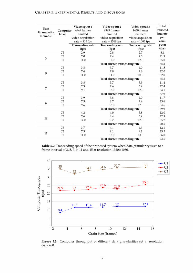
CHAPTER 5: EXPERIMENTAL RESULTS AND DISCUSSIONS
DataGranularity
(frames)
Computerlabel
Video spout 1 Video spout 2 Video spout 3 Totaltranscod-ing rate
percom-puter(fps)
4949 framesemitted
4949 framesemitted
4430 framesemitted
video acquisitionrate = 815 fps
video acquisitionrate = 1568 fps
video acquisitionrate = 1003 fps
Transcoding rate(fps)
Transcoding rate(fps)
Transcoding rate(fps)
3
C1 2.9 2.8 2.7 8.4C2 7.0 7.4 7.5 21.9C3 11.0 12.0 12.0 35.0
Total cluster transcoding rate 65.3
5
C1 3.8 3.7 4.0 11.5C2 7.4 7.0 7.6 22.0C3 11.0 11.0 10.0 32.0
Total cluster transcoding rate 65.5
7
C1 3.8 3.7 3.9 11.4C2 7.9 7.6 6.9 22.4C3 9.1 13.0 12.0 34.1
Total cluster transcoding rate 67.9
9
C1 3.9 3.8 4.0 11.7C2 7.5 8.7 7.4 23.6C3 9.6 13.0 12.0 34.6
Total cluster transcoding rate 69.9
11
C1 4.2 4.0 3.8 12.0C2 7.6 8.4 6.9 22.9C3 14.0 9.7 12.0 35.7
Total cluster transcoding rate 70.6
15
C1 3.7 4.1 4.3 12.1C2 7.3 9.1 9.1 25.5C3 11.0 12.0 13.0 36.0
Total cluster transcoding rate 73.6
Table 5.7: Transcoding speed of the proposed system when data granularity is set to aframe interval of 3, 5, 7, 9, 11 and 15 at resolution 1920×1080.
2 4 6 8 10 12 14 160
5
10
15
20
25
30
35
40
8.411.5 11.4 11.7 12 12.1
21.9 22 22.4 23.6 22.925.5
3532
34.1 34.6 35.7 36
Grain Size (frames)
Com
pute
rTh
roug
hput
(fps
)
C1C2C3
Figure 5.3: Computer throughput of different data granularities set at resolution640×480.
66
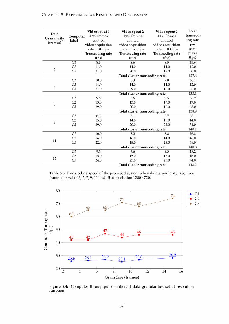
CHAPTER 5: EXPERIMENTAL RESULTS AND DISCUSSIONS
DataGranularity
(frames)
Computerlabel
Video spout 1 Video spout 2 Video spout 3 Totaltranscod-ing rate
percom-puter(fps)
4949 framesemitted
4949 framesemitted
4430 framesemitted
video acquisitionrate = 815 fps
video acquisitionrate = 1568 fps
video acquisitionrate = 1003 fps
Transcoding rate(fps)
Transcoding rate(fps)
Transcoding rate(fps)
3
C1 8.5 8.6 8.5 25.6C2 14.0 14.0 14.0 42.0C3 21.0 20.0 19.0 60.0
Total cluster transcoding rate 127.6
5
C1 10.0 8.3 7.8 26.1C2 14.0 14.0 14.0 42.0C3 21.0 29.0 15.0 65.0
Total cluster transcoding rate 133.1
7
C1 9.8 7.6 9.5 26.9C2 15.0 15.0 17.0 47.0C3 29.0 20.0 16.0 65.0
Total cluster transcoding rate 138.9
9
C1 8.3 8.1 8.7 25.1C2 15.0 14.0 15.0 44.0C3 29.0 20.0 22.0 71.0
Total cluster transcoding rate 140.1
11
C1 10.0 8.0 8.8 26.8C2 16.0 16.0 14.0 46.0C3 22.0 18.0 28.0 68.0
Total cluster transcoding rate 140.8
15
C1 9.3 9.6 9.3 28.2C2 15.0 15.0 16.0 46.0C3 24.0 25.0 25.0 74.0
Total cluster transcoding rate 148.2
Table 5.8: Transcoding speed of the proposed system when data granularity is set to aframe interval of 3, 5, 7, 9, 11 and 15 at resolution 1280×720.
2 4 6 8 10 12 14 1620
30
40
50
60
70
80
25.6 26.1 26.9 25.1 26.8 28.2
42 42
4744
46 46
60
65 65
7168
74
Grain Size (frames)
Com
pute
rTh
roug
hput
(fps
)
C1C2C3
Figure 5.4: Computer throughput of different data granularities set at resolution640×480.
67
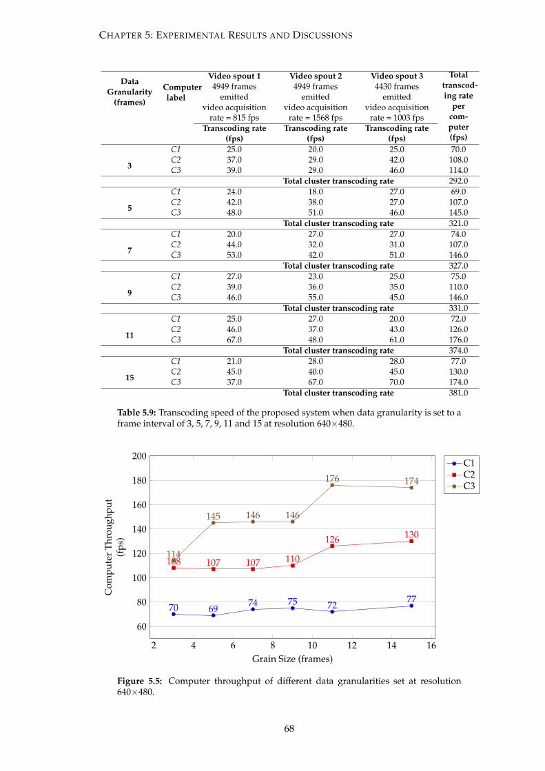
CHAPTER 5: EXPERIMENTAL RESULTS AND DISCUSSIONS
DataGranularity
(frames)
Computerlabel
Video spout 1 Video spout 2 Video spout 3 Totaltranscod-ing rate
percom-puter(fps)
4949 framesemitted
4949 framesemitted
4430 framesemitted
video acquisitionrate = 815 fps
video acquisitionrate = 1568 fps
video acquisitionrate = 1003 fps
Transcoding rate(fps)
Transcoding rate(fps)
Transcoding rate(fps)
3
C1 25.0 20.0 25.0 70.0C2 37.0 29.0 42.0 108.0C3 39.0 29.0 46.0 114.0
Total cluster transcoding rate 292.0
5
C1 24.0 18.0 27.0 69.0C2 42.0 38.0 27.0 107.0C3 48.0 51.0 46.0 145.0
Total cluster transcoding rate 321.0
7
C1 20.0 27.0 27.0 74.0C2 44.0 32.0 31.0 107.0C3 53.0 42.0 51.0 146.0
Total cluster transcoding rate 327.0
9
C1 27.0 23.0 25.0 75.0C2 39.0 36.0 35.0 110.0C3 46.0 55.0 45.0 146.0
Total cluster transcoding rate 331.0
11
C1 25.0 27.0 20.0 72.0C2 46.0 37.0 43.0 126.0C3 67.0 48.0 61.0 176.0
Total cluster transcoding rate 374.0
15
C1 21.0 28.0 28.0 77.0C2 45.0 40.0 45.0 130.0C3 37.0 67.0 70.0 174.0
Total cluster transcoding rate 381.0
Table 5.9: Transcoding speed of the proposed system when data granularity is set to aframe interval of 3, 5, 7, 9, 11 and 15 at resolution 640×480.
2 4 6 8 10 12 14 16
60
80
100
120
140
160
180
200
70 6974 75 72
77
108 107 107 110
126 130
114
145 146 146
176 174
Grain Size (frames)
Com
pute
rTh
roug
hput
(fps
)
C1C2C3
Figure 5.5: Computer throughput of different data granularities set at resolution640×480.
68
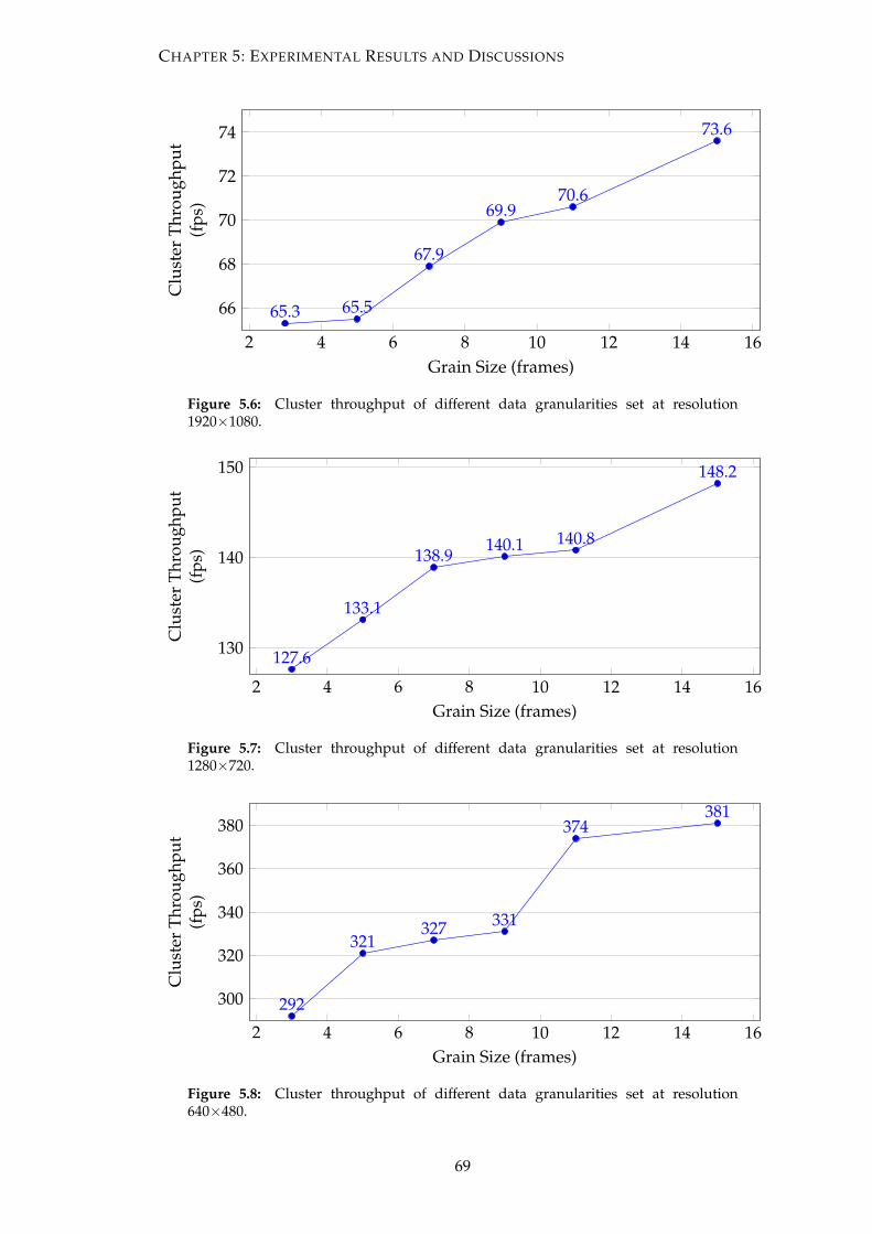
CHAPTER 5: EXPERIMENTAL RESULTS AND DISCUSSIONS
2 4 6 8 10 12 14 16
66
68
70
72
74
65.3 65.5
67.9
69.970.6
73.6
Grain Size (frames)
Clu
ster
Thro
ughp
ut(f
ps)
Figure 5.6: Cluster throughput of different data granularities set at resolution1920×1080.
2 4 6 8 10 12 14 16
130
140
150
127.6
133.1
138.9140.1 140.8
148.2
Grain Size (frames)
Clu
ster
Thro
ughp
ut(f
ps)
Figure 5.7: Cluster throughput of different data granularities set at resolution1280×720.
2 4 6 8 10 12 14 16
300
320
340
360
380
292
321327 331
374381
Grain Size (frames)
Clu
ster
Thro
ughp
ut(f
ps)
Figure 5.8: Cluster throughput of different data granularities set at resolution640×480.
69
CHAPTER 5: EXPERIMENTAL RESULTS AND DISCUSSIONS
5.3 Performance Evaluation of the Proposed Resource-Aware
Task Allocation Scheme
A resource-aware grouping strategy is implemented to reduce the impacts of system
heterogeneity to the proposed system. Three computers with their CPU specifications
listed in Table 5.1 were used in the experiment. Tables 5.10 to 5.12 demonstrate the
distribution of workload in Storm’s various stream grouping techniques. One can see
that by using the proposed resource-aware task allocation scheme onto either fields
grouping or the partial key grouping approach, the number of transcoded frames for
each computer is assigned in different amounts. Computers with higher transcoding
speed will receive more frames compared to the lower performance computers. This
is done by assigning the number of frames emitted for each supervisor based on their
computing ratios.
70
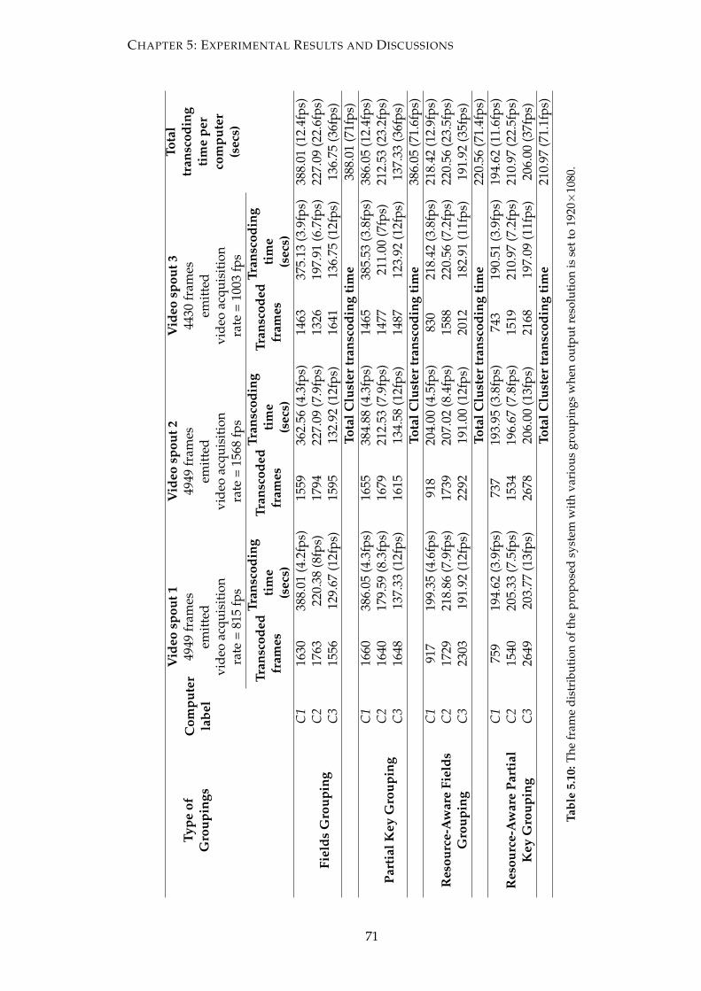
CHAPTER 5: EXPERIMENTAL RESULTS AND DISCUSSIONS
Type
ofG
roup
ings
Com
pute
rla
bel
Vid
eosp
out1
Vid
eosp
out2
Vid
eosp
out3
Tota
ltr
ansc
odin
gti
me
per
com
pute
r(s
ecs)
4949
fram
esem
itte
d49
49fr
ames
emit
ted
4430
fram
esem
itte
dvi
deo
acqu
isit
ion
rate
=81
5fp
svi
deo
acqu
isit
ion
rate
=15
68fp
svi
deo
acqu
isit
ion
rate
=10
03fp
s
Tran
scod
edfr
ames
Tran
scod
ing
tim
e(s
ecs)
T ran
scod
edfr
ames
Tran
scod
ing
tim
e(s
ecs)
Tran
scod
edfr
ames
Tran
scod
ing
tim
e(s
ecs)
Fiel
dsG
roup
ing
C1
1630
388.
01(4
.2fp
s)15
5936
2.56
(4.3
fps)
1463
375.
13(3
.9fp
s)38
8.01
(12.
4fps
)C
217
6322
0.38
(8fp
s)17
9422
7.09
(7.9
fps)
1326
197.
91(6
.7fp
s)22
7.09
(22.
6fps
)C
315
5612
9.67
(12f
ps)
1595
132.
92(1
2fps
)16
4113
6.75
(12f
ps)
136.
75(3
6fps
)To
talC
lust
ertr
ansc
odin
gti
me
388.
01(7
1fps
)
Part
ialK
eyG
roup
ing
C1
1660
386.
05(4
.3fp
s)16
5538
4.88
(4.3
fps)
1465
385.
53(3
.8fp
s)38
6.05
(12.
4fps
)C
216
4017
9.59
(8.3
fps)
1679
212.
53(7
.9fp
s)14
7721
1.00
(7fp
s)21
2.53
(23.
2fps
)C
316
4813
7.33
(12f
ps)
1615
134.
58(1
2fps
)14
8712
3.92
(12f
ps)
137.
33(3
6fps
)To
talC
lust
ertr
ansc
odin
gti
me
386.
05(7
1.6f
ps)
Res
ourc
e-A
war
eFi
elds
Gro
upin
g
C1
917
199.
35(4
.6fp
s)91
820
4.00
(4.5
fps)
830
218.
42(3
.8fp
s)21
8.42
(12.
9fps
)C
217
2921
8.86
(7.9
fps)
1739
207.
02(8
.4fp
s)15
8822
0.56
(7.2
fps)
220.
56(2
3.5f
ps)
C3
2303
191.
92(1
2fps
)22
9219
1.00
(12f
ps)
2012
182.
91(1
1fps
)19
1.92
(35f
ps)
Tota
lClu
ster
tran
scod
ing
tim
e22
0.56
(71.
4fps
)
Res
ourc
e-A
war
ePa
rtia
lK
eyG
roup
ing
C1
759
194.
62(3
.9fp
s)73
719
3.95
(3.8
fps)
743
190.
51(3
.9fp
s)19
4.62
(11.
6fps
)C
215
4020
5.33
(7.5
fps)
1534
196.
67(7
.8fp
s)15
1921
0.97
(7.2
fps)
210.
97(2
2.5f
ps)
C3
2649
203.
77(1
3fps
)26
7820
6.00
(13f
ps)
2168
197.
09(1
1fps
)20
6.00
(37f
ps)
Tota
lClu
ster
tran
scod
ing
tim
e21
0.97
(71.
1fps
)
Tabl
e5.
10:T
hefr
ame
dist
ribu
tion
ofth
epr
opos
edsy
stem
wit
hva
riou
sgr
oupi
ngs
whe
nou
tput
reso
luti
onis
sett
o19
20×
1080
.
71

CHAPTER 5: EXPERIMENTAL RESULTS AND DISCUSSIONS
Type
ofG
roup
ings
Com
pute
rla
bel
Vid
eosp
out1
Vid
eosp
out2
Vid
eosp
out3
Tota
ltr
ansc
odin
gti
me
per
com
pute
r(s
ecs)
4949
fram
esem
itte
d49
49fr
ames
emit
ted
4430
fram
esem
itte
dvi
deo
acqu
isit
ion
rate
=81
5fp
svi
deo
acqu
isit
ion
rate
=15
68fp
svi
deo
acqu
isit
ion
rate
=10
03fp
s
Tran
scod
edfr
ames
Tran
scod
ing
tim
e(s
ecs)
T ran
scod
edfr
ames
Tran
scod
ing
tim
e(s
ecs)
Tran
scod
edfr
ames
Tran
scod
ing
tim
e(s
ecs)
Fiel
dsG
roup
ing
C1
1597
185.
70(8
.6fp
s)15
8917
4.62
(9.1
fps)
1463
178.
41(8
.2fp
s)18
5.70
(26f
ps)
C2
1741
96.7
2(1
8fps
)17
9799
.83
(18f
ps)
1305
93.2
1(1
4fps
)99
.83
(50f
ps)
C3
1610
67.0
8(2
4fps
)15
8572
.05
(22f
ps)
1662
69.2
5(2
4fps
)72
.05
(70f
ps)
Tota
lClu
ster
tran
scod
ing
tim
e18
5.70
(146
fps)
Part
ialK
eyG
roup
ing
C1
1664
184.
89(9
fps)
1639
176.
24(9
.3fp
s)14
5818
2.25
(8fp
s)18
4.89
(26.
3fps
)C
216
5697
.41
(17f
ps)
1660
97.6
5(1
7fps
)14
8398
.87
(15f
ps)
98.8
7(4
9fps
)C
316
2865
.12
(25f
ps)
1650
71.7
4(2
3fps
)14
8867
.64
(22f
ps)
71.7
4(7
0fps
)To
talC
lust
ertr
ansc
odin
gti
me
184.
89(1
45.3
fps)
Res
ourc
e-A
war
eFi
elds
Gro
upin
g
C1
896
104.
19(8
.6fp
s)94
511
3.86
(8.3
fps)
812
105.
45(7
.7fp
s)11
3.86
(24f
ps)
C2
1735
108.
44(1
6fps
)17
4310
8.94
(16f
ps)
1576
105.
07(1
5fps
)10
8.94
(47f
ps)
C3
2318
96.5
8(2
4fps
)23
1096
.25
(24f
ps)
2042
92.8
2(2
2fps
)96
.58
(70f
ps)
Tota
lClu
ster
tran
scod
ing
tim
e11
3.86
(141
.6fp
s)
Res
ourc
e-A
war
ePa
rtia
lK
eyG
roup
ing
C1
894
113.
16(7
.9fp
s)89
011
4.10
(7.8
fps)
825
114.
58(7
.2fp
s)11
4.58
(22.
9fps
)C
217
2410
1.41
(17f
ps)
1728
96.0
0(1
8fps
)15
4410
2.93
(15f
ps)
102.
93(5
0fps
)C
323
2997
.04
(24f
ps)
2331
97.1
3(2
4fps
)20
6093
.64
(22f
ps)
97.1
3(7
0fps
)To
talC
lust
ertr
ansc
odin
gti
me
114.
58(1
43fp
s)
Tabl
e5.
11:T
hefr
ame
dist
ribu
tion
ofth
epr
opos
edsy
stem
wit
hva
riou
sgr
oupi
ngs
whe
nou
tput
reso
luti
onis
sett
o12
80×
720.
72
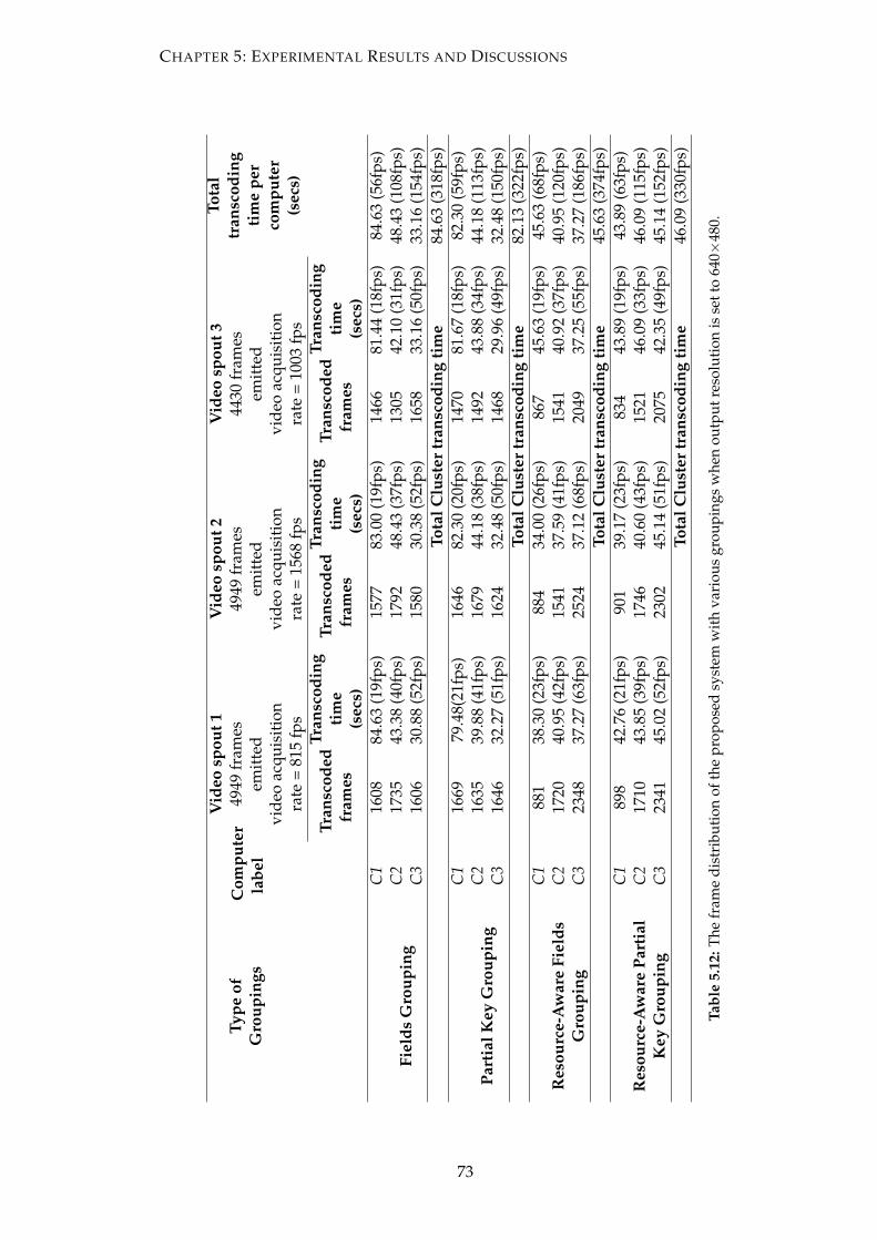
CHAPTER 5: EXPERIMENTAL RESULTS AND DISCUSSIONS
Type
ofG
roup
ings
Com
pute
rla
bel
Vid
eosp
out1
Vid
eosp
out2
Vid
eosp
out3
Tota
ltr
ansc
odin
gti
me
per
com
pute
r(s
ecs)
4949
fram
esem
itte
d49
49fr
ames
emit
ted
4430
fram
esem
itte
dvi
deo
acqu
isit
ion
rate
=81
5fp
svi
deo
acqu
isit
ion
rate
=15
68fp
svi
deo
acqu
isit
ion
rate
=10
03fp
s
Tran
scod
edfr
ames
Tran
scod
ing
tim
e(s
ecs)
T ran
scod
edfr
ames
Tran
scod
ing
tim
e(s
ecs)
Tran
scod
edfr
ames
Tran
scod
ing
tim
e(s
ecs)
Fiel
dsG
roup
ing
C1
1608
84.6
3(1
9fps
)15
7783
.00
(19f
ps)
1466
81.4
4(1
8fps
)84
.63
(56f
ps)
C2
1735
43.3
8(4
0fps
)17
9248
.43
(37f
ps)
1305
42.1
0(3
1fps
)48
.43
(108
fps)
C3
1606
30.8
8(5
2fps
)15
8030
.38
(52f
ps)
1658
33.1
6(5
0fps
)33
.16
(154
fps)
Tota
lClu
ster
tran
scod
ing
tim
e84
.63
(318
fps)
Part
ialK
eyG
roup
ing
C1
1669
79.4
8(21
fps)
1646
82.3
0(2
0fps
)14
7081
.67
(18f
ps)
82.3
0(5
9fps
)C
216
3539
.88
(41f
ps)
1679
44.1
8(3
8fps
)14
9243
.88
(34f
ps)
44.1
8(1
13fp
s)C
316
4632
.27
(51f
ps)
1624
32.4
8(5
0fps
)14
6829
.96
(49f
ps)
32.4
8(1
50fp
s)To
talC
lust
ertr
ansc
odin
gti
me
82.1
3(3
22fp
s)
Res
ourc
e-A
war
eFi
elds
Gro
upin
g
C1
881
38.3
0(2
3fps
)88
434
.00
(26f
ps)
867
45.6
3(1
9fps
)45
.63
(68f
ps)
C2
1720
40.9
5(4
2fps
)15
4137
.59
(41f
ps)
1541
40.9
2(3
7fps
)40
.95
(120
fps)
C3
2348
37.2
7(6
3fps
)25
2437
.12
(68f
ps)
2049
37.2
5(5
5fps
)37
.27
(186
fps)
Tota
lClu
ster
tran
scod
ing
tim
e45
.63
(374
fps)
Res
ourc
e-A
war
ePa
rtia
lK
eyG
roup
ing
C1
898
42.7
6(2
1fps
)90
139
.17
(23f
ps)
834
43.8
9(1
9fps
)43
.89
(63f
ps)
C2
1710
43.8
5(3
9fps
)17
4640
.60
(43f
ps)
1521
46.0
9(3
3fps
)46
.09
(115
fps)
C3
2341
45.0
2(5
2fps
)23
0245
.14
(51f
ps)
2075
42.3
5(4
9fps
)45
.14
(152
fps)
Tota
lClu
ster
tran
scod
ing
tim
e46
.09
(330
fps)
Tabl
e5.
12:T
hefr
ame
dist
ribu
tion
ofth
epr
opos
edsy
stem
wit
hva
riou
sgr
oupi
ngs
whe
nou
tput
reso
luti
onis
sett
o64
0×48
0.
73
CHAPTER 5: EXPERIMENTAL RESULTS AND DISCUSSIONS
5.4 Comparative Evaluation of Various Groupings to the Pro-
posed System
The load distribution of each grouping is plotted in Figures 5.9 to 5.20 and Figures 5.21
to 5.32 are plotted to illustrate the impacts of various groupings on the transcoding time
of the proposed system. In Storm’s default fields grouping and partial key grouping,
the transcoding time of the entire system is bounded by the worst-performing com-
puter C1 in the system when all GOP fragments are evenly distributed across heteroge-
neous computers in the Storm cluster. On the other hand, our proposed resource-aware
task allocation scheme implemented onto the Storm’s stream grouping strategies has
shown up to 44% performance improvement of the entire proposed system where in-
put GOP fragments are distributed strictly corresponding to the nodes’s computing
ratios in order to overcome performance degradation caused by system heterogeneity.
On the contrary, it is worth noting that partial key grouping is still the best approach
for distributing workload among computers with equal capabilities in homogeneous
systems.
74
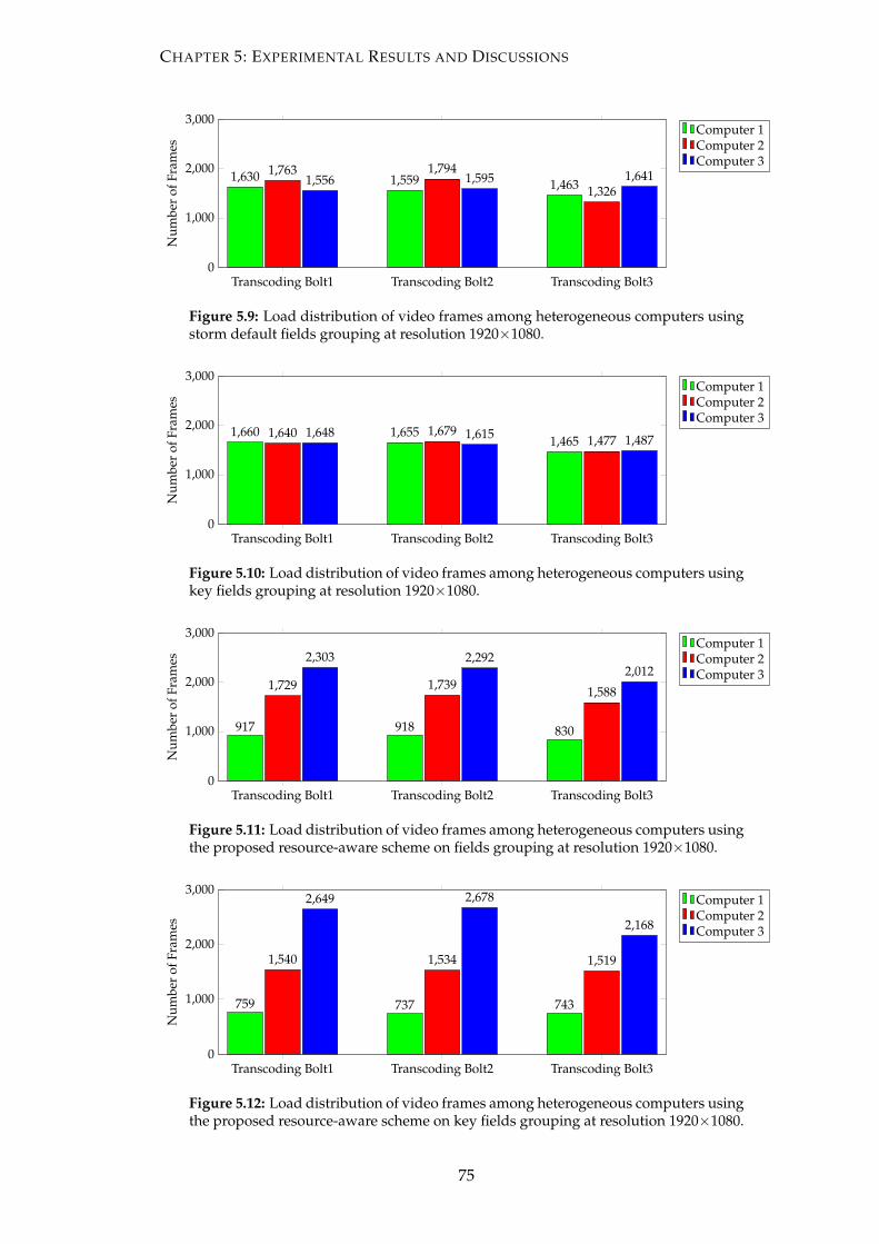
CHAPTER 5: EXPERIMENTAL RESULTS AND DISCUSSIONS
Transcoding Bolt1 Transcoding Bolt2 Transcoding Bolt30
1,000
2,000
3,000
1,630 1,559 1,4631,763 1,794
1,3261,556 1,595 1,641
Num
ber
ofFr
ames
Computer 1Computer 2Computer 3
Figure 5.9: Load distribution of video frames among heterogeneous computers usingstorm default fields grouping at resolution 1920×1080.
Transcoding Bolt1 Transcoding Bolt2 Transcoding Bolt30
1,000
2,000
3,000
1,660 1,6551,465
1,640 1,6791,477
1,648 1,615 1,487
Num
ber
ofFr
ames
Computer 1Computer 2Computer 3
Figure 5.10: Load distribution of video frames among heterogeneous computers usingkey fields grouping at resolution 1920×1080.
Transcoding Bolt1 Transcoding Bolt2 Transcoding Bolt30
1,000
2,000
3,000
917 918 830
1,729 1,739 1,588
2,303 2,2922,012
Num
ber
ofFr
ames
Computer 1Computer 2Computer 3
Figure 5.11: Load distribution of video frames among heterogeneous computers usingthe proposed resource-aware scheme on fields grouping at resolution 1920×1080.
Transcoding Bolt1 Transcoding Bolt2 Transcoding Bolt30
1,000
2,000
3,000
759 737 743
1,540 1,534 1,519
2,649 2,678
2,168
Num
ber
ofFr
ames
Computer 1Computer 2Computer 3
Figure 5.12: Load distribution of video frames among heterogeneous computers usingthe proposed resource-aware scheme on key fields grouping at resolution 1920×1080.
75
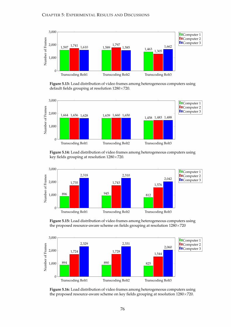
CHAPTER 5: EXPERIMENTAL RESULTS AND DISCUSSIONS
Transcoding Bolt1 Transcoding Bolt2 Transcoding Bolt30
1,000
2,000
3,000
1,597 1,589 1,4631,741 1,797
1,3051,610 1,585 1,662
Num
ber
ofFr
ames
Computer 1Computer 2Computer 3
Figure 5.13: Load distribution of video frames among heterogeneous computers usingdefault fields grouping at resolution 1280×720.
Transcoding Bolt1 Transcoding Bolt2 Transcoding Bolt30
1,000
2,000
3,000
1,664 1,6391,458
1,656 1,6601,4831,628 1,650
1,488
Num
ber
ofFr
ames
Computer 1Computer 2Computer 3
Figure 5.14: Load distribution of video frames among heterogeneous computers usingkey fields grouping at resolution 1280×720.
Transcoding Bolt1 Transcoding Bolt2 Transcoding Bolt30
1,000
2,000
3,000
896 945 812
1,735 1,7431,576
2,318 2,3102,042
Num
ber
ofFr
ames
Computer 1Computer 2Computer 3
Figure 5.15: Load distribution of video frames among heterogeneous computers usingthe proposed resource-aware scheme on fields grouping at resolution 1280×720
Transcoding Bolt1 Transcoding Bolt2 Transcoding Bolt30
1,000
2,000
3,000
894 890 825
1,724 1,7281,544
2,329 2,3312,060
Num
ber
ofFr
ames
Computer 1Computer 2Computer 3
Figure 5.16: Load distribution of video frames among heterogeneous computers usingthe proposed resource-aware scheme on key fields grouping at resolution 1280×720.
76
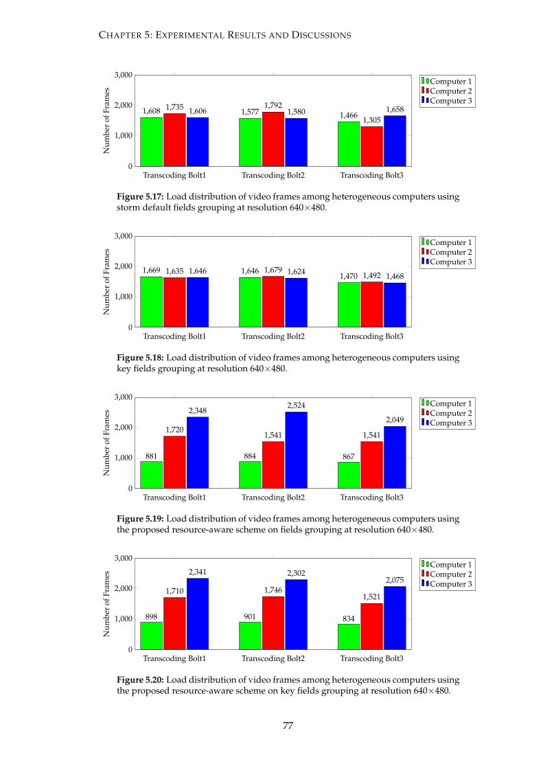
CHAPTER 5: EXPERIMENTAL RESULTS AND DISCUSSIONS
Transcoding Bolt1 Transcoding Bolt2 Transcoding Bolt30
1,000
2,000
3,000
1,608 1,577 1,4661,735 1,792
1,3051,606 1,580 1,658
Num
ber
ofFr
ames
Computer 1Computer 2Computer 3
Figure 5.17: Load distribution of video frames among heterogeneous computers usingstorm default fields grouping at resolution 640×480.
Transcoding Bolt1 Transcoding Bolt2 Transcoding Bolt30
1,000
2,000
3,000
1,669 1,6461,470
1,635 1,6791,4921,646 1,624 1,468
Num
ber
ofFr
ames
Computer 1Computer 2Computer 3
Figure 5.18: Load distribution of video frames among heterogeneous computers usingkey fields grouping at resolution 640×480.
Transcoding Bolt1 Transcoding Bolt2 Transcoding Bolt30
1,000
2,000
3,000
881 884 867
1,7201,541 1,541
2,3482,524
2,049
Num
ber
ofFr
ames
Computer 1Computer 2Computer 3
Figure 5.19: Load distribution of video frames among heterogeneous computers usingthe proposed resource-aware scheme on fields grouping at resolution 640×480.
Transcoding Bolt1 Transcoding Bolt2 Transcoding Bolt30
1,000
2,000
3,000
898 901 834
1,710 1,7461,521
2,341 2,3022,075
Num
ber
ofFr
ames
Computer 1Computer 2Computer 3
Figure 5.20: Load distribution of video frames among heterogeneous computers usingthe proposed resource-aware scheme on key fields grouping at resolution 640×480.
77
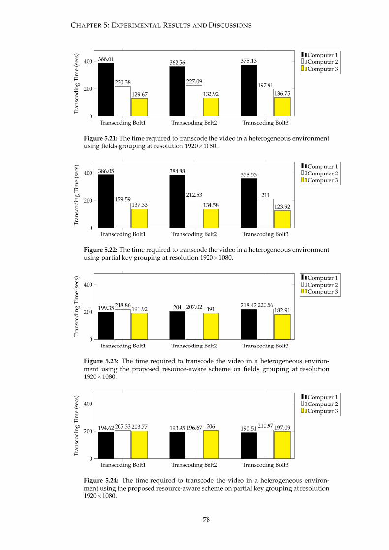
CHAPTER 5: EXPERIMENTAL RESULTS AND DISCUSSIONS
Transcoding Bolt1 Transcoding Bolt2 Transcoding Bolt30
200
400 388.01 362.56 375.13
220.38 227.09197.91
129.67 132.92 136.75
Tran
scod
ing
Tim
e(s
ecs) Computer 1
Computer 2Computer 3
Figure 5.21: The time required to transcode the video in a heterogeneous environmentusing fields grouping at resolution 1920×1080.
Transcoding Bolt1 Transcoding Bolt2 Transcoding Bolt30
200
400 386.05 384.88358.53
179.59212.53 211
137.33 134.58 123.92
Tran
scod
ing
Tim
e(s
ecs) Computer 1
Computer 2Computer 3
Figure 5.22: The time required to transcode the video in a heterogeneous environmentusing partial key grouping at resolution 1920×1080.
Transcoding Bolt1 Transcoding Bolt2 Transcoding Bolt30
200
400
199.35 204 218.42218.86 207.02 220.56191.92 191 182.91
Tran
scod
ing
T im
e(s
ecs) Computer 1
Computer 2Computer 3
Figure 5.23: The time required to transcode the video in a heterogeneous environ-ment using the proposed resource-aware scheme on fields grouping at resolution1920×1080.
Transcoding Bolt1 Transcoding Bolt2 Transcoding Bolt30
200
400
194.62 193.95 190.51205.33 196.67 210.97203.77 206 197.09
Tran
scod
ing
Tim
e(s
ecs) Computer 1
Computer 2Computer 3
Figure 5.24: The time required to transcode the video in a heterogeneous environ-ment using the proposed resource-aware scheme on partial key grouping at resolution1920×1080.
78
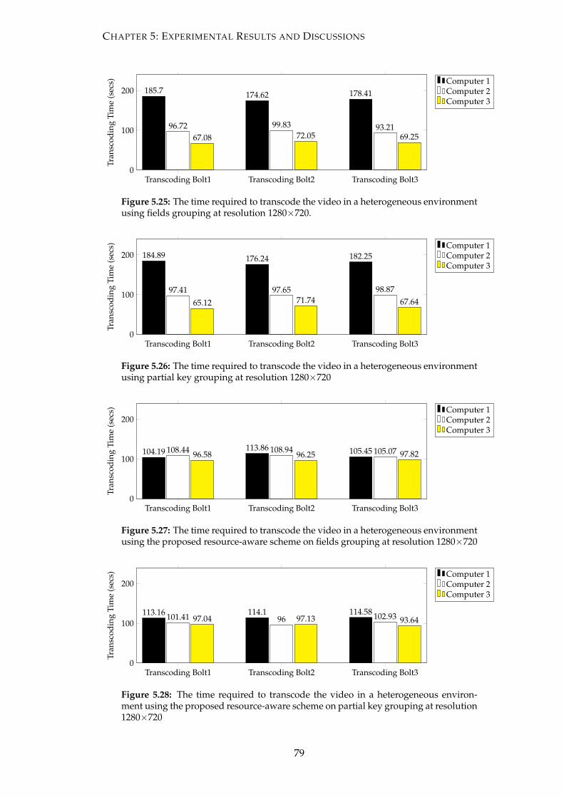
CHAPTER 5: EXPERIMENTAL RESULTS AND DISCUSSIONS
Transcoding Bolt1 Transcoding Bolt2 Transcoding Bolt30
100
200 185.7 174.62 178.41
96.72 99.83 93.2167.08 72.05 69.25
Tran
scod
ing
Tim
e(s
ecs) Computer 1
Computer 2Computer 3
Figure 5.25: The time required to transcode the video in a heterogeneous environmentusing fields grouping at resolution 1280×720.
Transcoding Bolt1 Transcoding Bolt2 Transcoding Bolt30
100
200 184.89 176.24 182.25
97.41 97.65 98.87
65.12 71.74 67.64
Tran
scod
ing
T im
e(s
ecs) Computer 1
Computer 2Computer 3
Figure 5.26: The time required to transcode the video in a heterogeneous environmentusing partial key grouping at resolution 1280×720
Transcoding Bolt1 Transcoding Bolt2 Transcoding Bolt30
100
200
104.19 113.86 105.45108.44 108.94 105.0796.58 96.25 97.82
Tran
scod
ing
Tim
e(s
ecs) Computer 1
Computer 2Computer 3
Figure 5.27: The time required to transcode the video in a heterogeneous environmentusing the proposed resource-aware scheme on fields grouping at resolution 1280×720
Transcoding Bolt1 Transcoding Bolt2 Transcoding Bolt30
100
200
113.16 114.1 114.58101.41 96 102.9397.04 97.13 93.64
Tran
scod
ing
T im
e(s
ecs) Computer 1
Computer 2Computer 3
Figure 5.28: The time required to transcode the video in a heterogeneous environ-ment using the proposed resource-aware scheme on partial key grouping at resolution1280×720
79
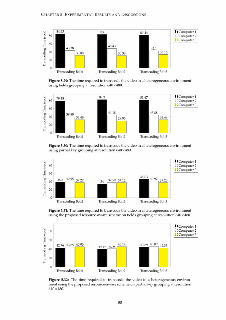
CHAPTER 5: EXPERIMENTAL RESULTS AND DISCUSSIONS
Transcoding Bolt1 Transcoding Bolt2 Transcoding Bolt30
20
40
60
8084.63 83 81.44
43.38 48.4342.1
30.88 30.38 33.16
Tran
scod
ing
Tim
e(s
ecs) Computer 1
Computer 2Computer 3
Figure 5.29: The time required to transcode the video in a heterogeneous environmentusing fields grouping at resolution 640×480.
Transcoding Bolt1 Transcoding Bolt2 Transcoding Bolt30
20
40
60
8079.48 82.3 81.67
39.88 44.18 43.8832.48 29.96 32.48
Tran
scod
ing
Tim
e(s
ecs) Computer 1
Computer 2Computer 3
Figure 5.30: The time required to transcode the video in a heterogeneous environmentusing partial key grouping at resolution 640×480.
Transcoding Bolt1 Transcoding Bolt2 Transcoding Bolt30
20
40
60
80
38.3 3445.6340.95 37.59 40.9237.27 37.12 37.25
Tran
scod
ing
Tim
e(s
ecs) Computer 1
Computer 2Computer 3
Figure 5.31: The time required to transcode the video in a heterogeneous environmentusing the proposed resource-aware scheme on fields grouping at resolution 640×480.
Transcoding Bolt1 Transcoding Bolt2 Transcoding Bolt30
20
40
60
80
42.76 39.1743.8943.85 40.6
46.0945.05 45.14 42.35
Tran
scod
ing
Tim
e(s
ecs)
Computer 1Computer 2Computer 3
Figure 5.32: The time required to transcode the video in a heterogeneous environ-ment using the proposed resource-aware scheme on partial key grouping at resolution640×480.
80
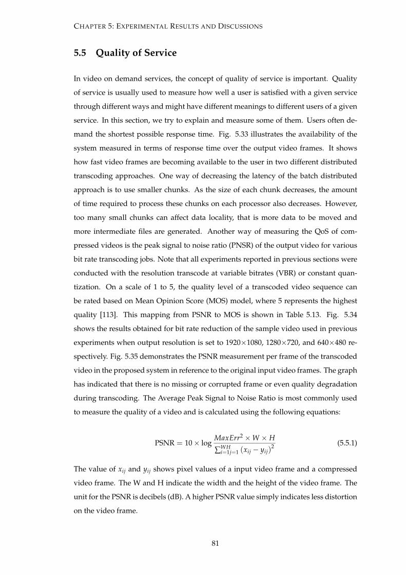
CHAPTER 5: EXPERIMENTAL RESULTS AND DISCUSSIONS
5.5 Quality of Service
In video on demand services, the concept of quality of service is important. Quality
of service is usually used to measure how well a user is satisfied with a given service
through different ways and might have different meanings to different users of a given
service. In this section, we try to explain and measure some of them. Users often de-
mand the shortest possible response time. Fig. 5.33 illustrates the availability of the
system measured in terms of response time over the output video frames. It shows
how fast video frames are becoming available to the user in two different distributed
transcoding approaches. One way of decreasing the latency of the batch distributed
approach is to use smaller chunks. As the size of each chunk decreases, the amount
of time required to process these chunks on each processor also decreases. However,
too many small chunks can affect data locality, that is more data to be moved and
more intermediate files are generated. Another way of measuring the QoS of com-
pressed videos is the peak signal to noise ratio (PNSR) of the output video for various
bit rate transcoding jobs. Note that all experiments reported in previous sections were
conducted with the resolution transcode at variable bitrates (VBR) or constant quan-
tization. On a scale of 1 to 5, the quality level of a transcoded video sequence can
be rated based on Mean Opinion Score (MOS) model, where 5 represents the highest
quality [113]. This mapping from PSNR to MOS is shown in Table 5.13. Fig. 5.34
shows the results obtained for bit rate reduction of the sample video used in previous
experiments when output resolution is set to 1920×1080, 1280×720, and 640×480 re-
spectively. Fig. 5.35 demonstrates the PSNR measurement per frame of the transcoded
video in the proposed system in reference to the original input video frames. The graph
has indicated that there is no missing or corrupted frame or even quality degradation
during transcoding. The Average Peak Signal to Noise Ratio is most commonly used
to measure the quality of a video and is calculated using the following equations:
PSNR = 10× logMaxErr2 ×W × H
∑WHi=1j=1 (xij − yij)
2 (5.5.1)
The value of xij and yij shows pixel values of a input video frame and a compressed
video frame. The W and H indicate the width and the height of the video frame. The
unit for the PSNR is decibels (dB). A higher PSNR value simply indicates less distortion
on the video frame.
81
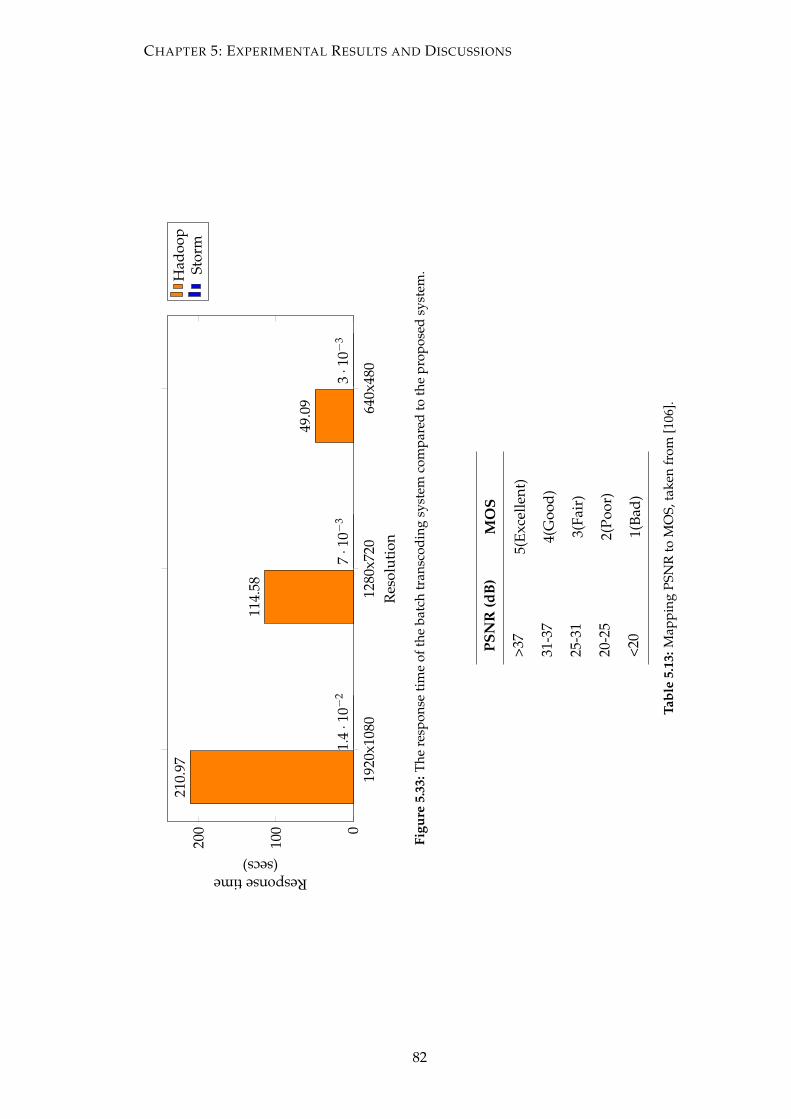
CHAPTER 5: EXPERIMENTAL RESULTS AND DISCUSSIONS
1920
x108
012
80x7
2064
0x48
00
100
200
210.
97
114.
58
49.0
9
1.4·1
0−2
7·1
0−3
3·1
0−3
Res
olut
ion
Responsetime(secs)
Had
oop
Stor
m
Figu
re5.
33:T
here
spon
seti
me
ofth
eba
tch
tran
scod
ing
syst
emco
mpa
red
toth
epr
opos
edsy
stem
.
PSN
R(d
B)
MO
S
>37
5(Ex
celle
nt)
31-3
74(
Goo
d)
25-3
13(
Fair
)
20-2
52(
Poor
)
<20
1(Ba
d)
Tabl
e5.
13:M
appi
ngPS
NR
toM
OS,
take
nfr
om[1
06].
82
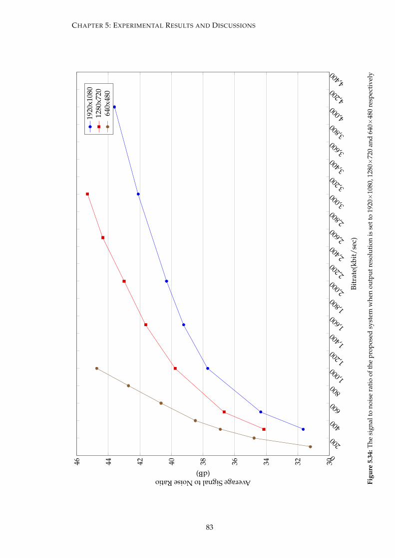
CHAPTER 5: EXPERIMENTAL RESULTS AND DISCUSSIONS
0
200
400
600
800
1,000
1,200
1,400
1,600
1,800
2,000
2,200
2,400
2,600
2,800
3,000
3,200
3,400
3,600
3,800
4,000
4,200
4,400
303234363840424446
Bitr
ate(
kbit
/sec
)
AverageSignaltoNoiseRatio(dB)
1920
x108
012
80x7
2064
0x48
0
Figu
re5.
34:T
hesi
gnal
tono
ise
rati
oof
the
prop
osed
syst
emw
hen
outp
utre
solu
tion
isse
tto
1920×
1080
,128
0×72
0an
d64
0×48
0re
spec
tive
ly
83
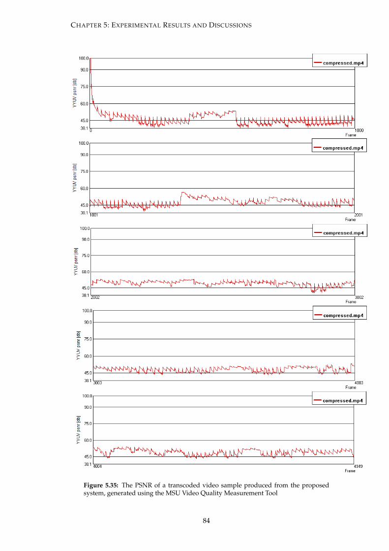
CHAPTER 5: EXPERIMENTAL RESULTS AND DISCUSSIONS
Figure 5.35: The PSNR of a transcoded video sample produced from the proposedsystem, generated using the MSU Video Quality Measurement Tool
84
CHAPTER 6
Conclusion and Future Works
6.1 Conclusion
In this work, we have proposed a distributed real-time video transcoding system, op-
erated on a heterogeneous computing platform. The proposed system is devised pri-
marily with real-time purposes that would be potentially useful for transcoding of live
streams at greater scale and speed which is demanding in today's large-scale video
surveillance system. Since input video streams are distributed to multiple computers
and all computers are utilized under the proposed system, the CPU load of all com-
puters can be reduced in real time. In the context of a large-scale video transcoding
system, more input video streams can be processed in such system.
Experiments have shown the practicality of the proposed system implemented on Apache
Storm. However, we found that the task allocation scheme used by Storm does not ef-
fectively distribute video frames among computers in heterogeneous systems accord-
ing to their processing powers, resulting in bottleneck in the overall transcoding time.
Subsequently, a resource-aware task allocation scheme is proposed and has overall re-
duced the amount of tasks allocated for the poor processing computer among hetero-
geneous computers. The proposed scheme has exhibited a good load balance of tasks
based on computing ratios, reducing the overall transcoding completion time of the
proposed system significantly.
Another key aspect when designing the proposed system is data granularity. A coarser
grain approach with micro batches of 15 frames GOP length has shown maximum
throughput and consistency achieved, having the same throughput as each computer
benchmarked under their local data. This method suggests that the data locality is not
85
CHAPTER 6: CONCLUSION AND FUTURE WORKS
a concern in affecting the acquiring throughput of the proposed system when a coarser
grain approach is used in data transmission. However, the performance of the pro-
posed system can suffer from load imbalance in a homogeneous environment if the
data is too coarse. This issue has been addressed by Nasir, Muhammad Anis Uddin, et
al. [111] using the partial key grouping strategy.
6.2 Future Work
Large-scale video transcoding systems in the field of distributed computing have at-
tracted increasing research interests in the last decade. As data intensive computing
problems evolve, there are many research activities and a series of issues remain to
be unsolved. Due to time and resource constraints, there are other interesting re-
search challenges such as an online resource-aware task allocation scheme, an intel-
ligent resource-aware scheduler and incorporation of hardware accelerators could be
subjected to further studies.
6.2.1 Online Resource-Aware GOP Allocation
Since the transcoding rate may vary slightly during the transcoding process, an of-
fline resource allocation scheme is not intelligent enough to dynamically allocate tasks
on-the-fly based on changed computing ratios. Therefore, the proposed future work
is to allow video frames to be dynamically assigned to computers according to their
processing capabilities to further optimize the system performance.
6.2.2 A Resource-Aware Scheduler
Similar to many other stream processing systems, Storm has been in the absence of
an intelligent scheduling mechanism to deal with heterogeneous systems. The cur-
rent default round-robin scheduler deployed in Storm neglects resource demands and
availability, and therefore can be inefficient in continuous run applications. R-Storm
is then proposed in [114] to maximize resource utilization while minimizing the net-
work latency and therefore increases the overall throughput of the system. In order
to maximize the utilization of every resource while minimizing the network distance
when scheduling tasks, the R-Storm scheduler efficiently schedules tasks closely to-
gether with their heterogeneous resource demands. This is true as scheduling every
86
CHAPTER 6: CONCLUSION AND FUTURE WORKS
spout task onto low performance but high memory machines will eventually increase
the processing throughput for the rest of the computation systems since more resource
availabilities are preserved. On the other hand, data locality is one of the widely
adopted scheduler decision in parallel systems. For example, the MapReduce frame-
work performs computation on a node where the required data is stored in order to
avoid intensive data loading and removal within the cluster. However, data locality
decisions from stream processing have different perspectives from batch processing as
stream processing often computes on streams coming from remote sources such as IP
cameras instead of static data that is stored locally or in the cluster. Hence, R-Storm has
considered data locality to be an effective strategy to minimize communication costs by
scheduling processor instances and data to be processed together on the same node or
nodes in the same rack.
6.2.3 Incorporation of GPU’s Parallel Processing to The Proposed System
In addition, GPU implementation of video transcoding can be incorporated for better
performance. We have experienced throughput degradation of the Nvidia Hardware
Encoder (NVENC) when using fine-grain or intra frame transcoding in Storm. There is
a number of challenges in making efficient GPU utilization in Storm. To achieve high
throughput, stream applications have to make use of batching strategies. Transferring
larger bulks of data (GOP size in our case) in between the cluster, GPUs and CPUs
can improve the GOP acquiring throughput. The distribution of frames in batches
also affects load balancing on GPUs if the data is too coarse. To achieve maximum
utilization of the whole system, distribution of workload between CPUs and GPUs has
to be considered.
87
Bibliography
[1] H Koumaras, C Skianis, G Gardikis, and A Kourtis. Analysis of h. 264 video en-
coded traffic. In Proceedings of the 5th International Network Conference (INC2005),
pages 441–448, 2005.
[2] NVIDIA. nvenc, nvidia gpu video encoding capabilities.
[3] Magor Corporation. The aerus service delivery platform, 1999.
[4] Konstantin Shvachko, Hairong Kuang, Sanjay Radia, and Robert Chansler. The
hadoop distributed file system. In 2010 IEEE 26th symposium on mass storage sys-
tems and technologies (MSST), pages 1–10. IEEE, 2010.
[5] Ankit Toshniwal, Siddarth Taneja, Amit Shukla, Karthik Ramasamy, Jignesh M
Patel, Sanjeev Kulkarni, Jason Jackson, Krishna Gade, Maosong Fu, Jake Don-
ham, et al. Storm@ twitter. In Proceedings of the 2014 ACM SIGMOD international
conference on Management of data, pages 147–156. ACM, 2014.
[6] Xinyao Zhang. The Analysis of Parallelism of Apache Storm. PhD thesis, Concordia
University, 2016.
[7] Fatih Porikli, François Brémond, Shiloh L Dockstader, James Ferryman, Anthony
Hoogs, Brian C Lovell, Sharath Pankanti, Bernhard Rinner, Peter Tu, Péter L
Venetianer, et al. Video surveillance: past, present, and now the future. IEEE
Signal Processing Magazine, 30(3):190–198, 2013.
[8] DJ Neal and Shawon Rahman. Video surveillance in the cloud. arXiv preprint
arXiv:1512.00070, 2015.
[9] Henning Schulzrinne. Real time streaming protocol (rtsp). 1998.
[10] World Wide Web Consortium et al. Html5 specification. Technical Specification,
Jun, 24:2010, 2010.
88
BIBLIOGRAPHY
[11] ONVIF. Core specification, 2012.
[12] Yucheng Low, Danny Bickson, Joseph Gonzalez, Carlos Guestrin, Aapo Kyrola,
and Joseph M Hellerstein. Distributed graphlab: a framework for machine learn-
ing and data mining in the cloud. Proceedings of the VLDB Endowment, 5(8):716–
727, 2012.
[13] Cheng Chu, Sang Kyun Kim, Yi-An Lin, YuanYuan Yu, Gary Bradski, Andrew Y
Ng, and Kunle Olukotun. Map-reduce for machine learning on multicore. Ad-
vances in neural information processing systems, 19:281, 2007.
[14] Min Chen, Shiwen Mao, and Yunhao Liu. Big data: a survey. Mobile Networks and
Applications, 19(2):171–209, 2014.
[15] Jeongnam Youn, Jun Xin, and Ming-Ting Sun. Fast video transcoding architec-
tures for networked multimedia applications. In Circuits and Systems, 2000. Pro-
ceedings. ISCAS 2000 Geneva. The 2000 IEEE International Symposium on, volume 4,
pages 25–28. IEEE, 2000.
[16] Ishfaq Ahmad, Xiaohui Wei, Yu Sun, and Ya-Qin Zhang. Video transcoding: an
overview of various techniques and research issues. IEEE Transactions on multi-
media, 7(5):793–804, 2005.
[17] Mathias Wien. Video coding fundamentals. In High Efficiency Video Coding, pages
23–71. Springer, 2015.
[18] Stephan Wenger and Thomas Stockhammer. Rtp payload format for h. 264 video.
2005.
[19] Tatjana Welzer, Hannu Jaakkola, and Bernhard Thalheim. Information Modelling
and Knowledge Bases XXVII, volume 280. Ios Press, 2016.
[20] Ming-Ting Sun. Compressed video over networks. CRC Press, 2000.
[21] Harkirat Singh, Chang Yeul Kwon, Seong Soo Kim, and Chiu Ngo. Iptv over
wirelesslan: promises and challenges. In 2008 5th IEEE Consumer Communications
and Networking Conference, pages 626–631. IEEE, 2008.
[22] Heiko Schwarz, Detlev Marpe, and Thomas Wiegand. Analysis of hierarchical b
pictures and mctf. In 2006 IEEE International Conference on Multimedia and Expo,
pages 1929–1932. IEEE, 2006.
89
BIBLIOGRAPHY
[23] On-Net Surveillance Systems Inc. Mjpeg vs mpeg4 understanding the differ-
ences, advantages and disadvantages of each compression technique. 2012.
[24] Didier Le Gall. Mpeg: A video compression standard for multimedia applica-
tions. Communications of the ACM, 34(4):46–58, 1991.
[25] Atul Puri. Video coding using the mpeg-2 compression standard. In Visual Com-
munications’ 93, pages 1701–1713. International Society for Optics and Photonics,
1993.
[26] Thierry Alpert, Vittorio Baroncini, Diana Choi, Laura Contin, Rob Koenen, Fer-
nando Pereira, and H Peterson. Subjective evaluation of mpeg-4 video codec
proposals: Methodological approach and test procedures. Signal Processing: Im-
age Communication, 9(4):305–325, 1997.
[27] Thomas Wiegand, Gary J Sullivan, Gisle Bjontegaard, and Ajay Luthra.
Overview of the h. 264/avc video coding standard. IEEE Transactions on circuits
and systems for video technology, 13(7):560–576, 2003.
[28] High Efficiency Video Coding. H. 265 and iso, 2013.
[29] Oliver Morgan. Wrappers and metadata sub group [digital video standards].
In The EBU-SMPTE Task Force: Building an Infrastructure for Managing Compressed
Video Systems (Ref. No: 1997/382), IEE Colloquium on, pages 5–1. IET, 1997.
[30] AMWA. A quick tour of wrappers and mxf. 2002.
[31] Source Wikipedia. Container Formats: Vqa, 3gp and 3g2, Adobe Captivate, Advanced
Systems Format, Anim, Annodex. University-Press Org, 2013.
[32] Sridhar Srinivasan, Pohsiang John Hsu, Tom Holcomb, Kunal Mukerjee,
Shankar L Regunathan, Bruce Lin, Jie Liang, Ming-Chieh Lee, and Jordi Ribas-
Corbera. Windows media video 9: overview and applications. Signal Processing:
Image Communication, 19(9):851–875, 2004.
[33] Eric Fleischman. Wave and avi codec registries. 1998.
[34] Alexander Noé. Matroska file format (under construction!). Jun, 24:1–51, 2007.
[35] Fernando CN Pereira and Touradj Ebrahimi. The MPEG-4 book. Prentice Hall
Professional, 2002.
90
BIBLIOGRAPHY
[36] Macromedia Flash. and flash video (flv) file format specification version 8, 2006.
[37] D Singer. 3gpp ts 26.244; transparent end-to-end packet switched streaming ser-
vice (pss); 3gpp file format (3gp), etsi 3gpp std., rev. 12.3. 0, march 2014, 2014.
[38] Anthony Vetro, Charilaos Christopoulos, and Huifang Sun. Video transcod-
ing architectures and techniques: an overview. IEEE signal processing magazine,
20(2):18–29, 2003.
[39] Jun Xin, Chia-Wen Lin, and Ming-Ting Sun. Digital video transcoding. Proceed-
ings of the IEEE, 93(1):84–97, 2005.
[40] Bo Shen, Wai-Tian Tan, and Frederic Huve. Dynamic video transcoding in mobile
environments. IEEE MultiMedia, 15(1):42–51, 2008.
[41] Martin Alexander Wilhelmsen, Håkon Kvale Stensland, Vamsidhar Reddy Gad-
dam, Asgeir Mortensen, Ragnar Langseth, Carsten Griwodz, and Pål Halvorsen.
Using a commodity hardware video encoder for interactive video streaming. In
Multimedia (ISM), 2014 IEEE International Symposium on, pages 251–254. IEEE,
2014.
[42] NVIDIA. Nvidia video encoder application note.
[43] NVIDIA. Video capture, encoding, and streaming in a multi-gpu system. Tech-
nical Report TB-05566-001-v01, 2010.
[44] Song Lin, Xinfeng Zhang, Qin Yu, Honggang Qi, and Siwei Ma. Parallelizing
video transcoding with load balancing on cloud computing. In 2013 IEEE Inter-
national Symposium on Circuits and Systems (ISCAS2013), pages 2864–2867. IEEE,
2013.
[45] Jeffrey Dean and Sanjay Ghemawat. Mapreduce: simplified data processing on
large clusters. Communications of the ACM, 51(1):107–113, 2008.
[46] Vinod Kumar Vavilapalli, Arun C Murthy, Chris Douglas, Sharad Agarwal, Ma-
hadev Konar, Robert Evans, Thomas Graves, Jason Lowe, Hitesh Shah, Siddharth
Seth, et al. Apache hadoop yarn: Yet another resource negotiator. In Proceedings
of the 4th annual Symposium on Cloud Computing, page 5. ACM, 2013.
[47] Nikolay Laptev, Kai Zeng, and Carlo Zaniolo. Very fast estimation for result and
accuracy of big data analytics: The earl system. In Data Engineering (ICDE), 2013
IEEE 29th International Conference on, pages 1296–1299. IEEE, 2013.
91
BIBLIOGRAPHY
[48] Jiong Xie, Shu Yin, Xiaojun Ruan, Zhiyang Ding, Yun Tian, James Majors, Adam
Manzanares, and Xiao Qin. Improving mapreduce performance through data
placement in heterogeneous hadoop clusters. In Parallel & Distributed Processing,
Workshops and Phd Forum (IPDPSW), 2010 IEEE International Symposium on, pages
1–9. IEEE, 2010.
[49] Tao Gu, Chuang Zuo, Qun Liao, Yulu Yang, and Tao Li. Improving mapreduce
performance by data prefetching in heterogeneous or shared environments. In-
ternational Journal of Grid & Distributed Computing, 6(5), 2013.
[50] Olli Lehtoranta, Erno Salminen, Ari Kulmala, Marko Hannikainen, and Timo D
Hamalainen. A parallel mpeg-4 encoder for fpga based multiprocessor soc. In
International Conference on Field Programmable Logic and Applications, 2005., pages
380–385. IEEE, 2005.
[51] Zhibin Xiao, Stephen Le, and Bevan Baas. A fine-grained parallel implemen-
tation of a h. 264/avc encoder on a 167-processor computational platform. In
2011 Conference Record of the Forty Fifth Asilomar Conference on Signals, Systems and
Computers (ASILOMAR), pages 2067–2071. IEEE, 2011.
[52] Kyoung Ill Kim, Su Young Bae, Dong Chun Lee, Chang Sik Cho, Hun Joo Lee,
and Kyu Chul Lee. Cloud-based gaming service platform supporting multiple
devices. ETRI Journal, 35(6):960–968, 2013.
[53] Svetislav Momcilovic, Aleksandar Ilic, Nuno Roma, and Leonel Sousa. Efficient
parallel video encoding on heterogeneous systems. 2014.
[54] Youngsub Ko, Youngmin Yi, and Soonhoi Ha. An efficient parallelization tech-
nique for x264 encoder on heterogeneous platforms consisting of cpus and gpus.
Journal of real-time image processing, 9(1):5–18, 2014.
[55] NVIDIA. nvenc, nvidia kepler hardware video encoder.
[56] Håkon Kvale Stensland, Martin Alexander Wilhelmsen, Vamsidhar Reddy Gad-
dam, Asgeir Mortensen, Ragnar Langseth, Carsten Griwodz, and Pål Halvorsen.
Using a commodity hardware video encoder for interactive applications. Interna-
tional Journal of Multimedia Data Engineering and Management (IJMDEM), 6(3):17–
31, 2015.
92
BIBLIOGRAPHY
[57] H Schwarz, T Hinz, H Kirchhoffer, D Marpe, and T Wiegand. Technical descrip-
tion of the hhi proposal for svc ce1. iso. Technical report, IEC JTC1/SC29/WG11,
Document, 2004.
[58] Heiko Schwarz, Detlev Marpe, and Thomas Wiegand. Overview of the scalable
video coding extension of the h. 264/avc standard. IEEE Transactions on circuits
and systems for video technology, 17(9):1103–1120, 2007.
[59] ISO ITU-T and IEC JTC. Generic coding of moving pictures and associated audio
information-part 2: video, 1995.
[60] Adrian Grange and Harald Alvestrand. A vp9 bitstream overview. 2013.
[61] Jim Bankoski, Paul Wilkins, and Yaowu Xu. Technical overview of vp8, an open
source video codec for the web. In ICME, pages 1–6, 2011.
[62] Dan Grois, Detlev Marpe, Amit Mulayoff, Benaya Itzhaky, and Ofer Hadar. Per-
formance comparison of h. 265/mpeg-hevc, vp9, and h. 264/mpeg-avc encoders.
In Picture Coding Symposium (PCS), 2013, pages 394–397. IEEE, 2013.
[63] Karine Pires and Gwendal Simon. Dash in twitch: Adaptive bitrate streaming
in live game streaming platforms. In Proceedings of the 2014 Workshop on Design,
Quality and Deployment of Adaptive Video Streaming, pages 13–18. ACM, 2014.
[64] Ramon Aparicio-Pardo, Karine Pires, Alberto Blanc, and Gwendal Simon.
Transcoding live adaptive video streams at a massive scale in the cloud. In Pro-
ceedings of the 6th ACM Multimedia Systems Conference, pages 49–60. ACM, 2015.
[65] Guntur Ravindra, Sumit Kumar, and Suresh Chintada. Distributed media
transcoding using a p2p network of set top boxes. In 2009 6th IEEE Consumer
Communications and Networking Conference, pages 1–2. IEEE, 2009.
[66] Can Yang, Yuanqiong Chen, and Yilong Shen. The research on a p2p transcoding
system based on distributed farming computing architecture. In Knowledge Engi-
neering and Software Engineering, 2009. KESE’09. Pacific-Asia Conference on, pages
55–58. IEEE, 2009.
[67] Dongyu Liu, Eric Setton, Bo Shen, and Songqing Chen. Pat: Peer-assisted
transcoding for overlay streaming to heterogeneous devices. In Proc. Int. Work-
shop Netw. Oper. Syst. Support Dig. Audio Video, 2007.
93
BIBLIOGRAPHY
[68] SPT Krishnan and Jose L Ugia Gonzalez. Google compute engine. In Building
Your Next Big Thing with Google Cloud Platform, pages 53–81. Springer, 2015.
[69] Amazon Elastic Compute Cloud. Amazon web services. Retrieved November,
9:2011, 2011.
[70] Sriram Krishnan. Programming Windows Azure: Programming the Microsoft Cloud.
" O’Reilly Media, Inc.", 2010.
[71] Minthu Ram Chiary and R Anand. Hadoop cluster on linode using ambari for
improvingtask assignment scheme running in the clouds.
[72] Zhiran Wang. Research on cloud computing-based online payment mode. In
Multimedia Information Networking and Security (MINES), 2011 Third International
Conference on, pages 559–563. IEEE, 2011.
[73] Jim Duval. My boss wants to transcode in the cloud. In SMPTE 2015 Annual
Technical Conference and Exhibition, pages 1–6. SMPTE, 2015.
[74] Adriana Garcia, Hari Kalva, and Borko Furht. A study of transcoding on cloud
environments for video content delivery. In Proceedings of the 2010 ACM multime-
dia workshop on Mobile cloud media computing, pages 13–18. ACM, 2010.
[75] Zhenhua Li, Yan Huang, Gang Liu, Fuchen Wang, Zhi-Li Zhang, and Yafei
Dai. Cloud transcoder: Bridging the format and resolution gap between inter-
net videos and mobile devices. In Proceedings of the 22nd international workshop
on Network and Operating System Support for Digital Audio and Video, pages 33–38.
ACM, 2012.
[76] Vijay Kumar Adhikari, Yang Guo, Fang Hao, Matteo Varvello, Volker Hilt, Moritz
Steiner, and Zhi-Li Zhang. Unreeling netflix: Understanding and improving
multi-cdn movie delivery. In INFOCOM, 2012 Proceedings IEEE, pages 1620–1628.
IEEE, 2012.
[77] Myoungjin Kim, Hanku Lee, Hyeokju Lee, and Seungho Han. Distributed video
transcoding system based on mapreduce for video content delivery, 2012.
[78] Haoyu Xu, Liangyou Wang, and Huang Xie. Design and experiment analysis
of a hadoop-based video transcoding system for next-generation wireless sensor
networks. International Journal of Distributed Sensor Networks, 2014, 2014.
94
BIBLIOGRAPHY
[79] Rainer Schmidt and Matthias Rella. An approach for processing large and non-
uniform media objects on mapreduce-based clusters. In International Conference
on Asian Digital Libraries, pages 172–181. Springer, 2011.
[80] Chenwei Song, Wenfeng Shen, Lianqiang Sun, Zhou Lei, and Weimin Xu. Dis-
tributed video transcoding based on mapreduce. In Computer and Information Sci-
ence (ICIS), 2014 IEEE/ACIS 13th International Conference on, pages 309–314. IEEE,
2014.
[81] F. Lao, X. Zhang, and Z. Guo. Parallelizing video transcoding using map-reduce-
based cloud computing. In 2012 IEEE International Symposium on Circuits and
Systems, pages 2905–2908, May 2012.
[82] Myoungjin Kim, Seungho Han, Yun Cui, Hanku Lee, and Changsung Jeong. Per-
formance optimization of a distributed transcoding system based on hadoop for
multimedia streaming services. International Information Institute (Tokyo). Informa-
tion, 18(5B):2099, 2015.
[83] Shyam Nandan Kumar. Advanced mechanism to handle big data of hd video
file for mobile devices. International Journal of Research in Engineering Technology
and Management, Paper Id: IJRETM-2014-02-06-006, 2(06):1–7, 2014.
[84] D Kesavaraja and A Shenbagavalli. Hadoop scalable video transcoding tech-
nique in cloud environment. In Intelligent Systems and Control (ISCO), 2015 IEEE
9th International Conference on, pages 1–6. IEEE, 2015.
[85] Akhmedov Khumoyun, Myoungjin Kim, Yun Cui, Seungho Han, Seunghyun
Seo, Seungbum Seo, and Hanku Lee. A study on multimedia transcoding ap-
proach by applying multiple mapreduce jobs. 2014.
[86] Myoungjin Kim, Yun Cui, Seungho Han, and Hanku Lee. Towards efficient de-
sign and implementation of a hadoop-based distributed video transcoding sys-
tem in cloud computing environment. International Journal of Multimedia and
Ubiquitous Engineering, 8(2):213–224, 2013.
[87] Fan Yang and Qi-Wei Shen. Distributed video transcoding on hadoop. Computer
Systems & Applications, 20(11):80–85, 2011.
[88] Rafael Pereira, Marcello Azambuja, Karin Breitman, and Markus Endler. An ar-
chitecture for distributed high performance video processing in the cloud. In
95
BIBLIOGRAPHY
2010 IEEE 3rd International Conference on Cloud Computing, pages 482–489. IEEE,
2010.
[89] Horacio Sanson, Luis Loyola, and Daniel Pereira. Scalable distributed architec-
ture for media transcoding. In International Conference on Algorithms and Architec-
tures for Parallel Processing, pages 288–302. Springer, 2012.
[90] Jorda Polo, Claris Castillo, David Carrera, Yolanda Becerra, Ian Whalley, Mal-
gorzata Steinder, Jordi Torres, and Eduard Ayguadé. Resource-aware adaptive
scheduling for mapreduce clusters. In ACM/IFIP/USENIX International Conference
on Distributed Systems Platforms and Open Distributed Processing, pages 187–207.
Springer, 2011.
[91] Raouf Boutaba, Lu Cheng, and Qi Zhang. On cloud computational models and
the heterogeneity challenge. Journal of Internet Services and Applications, 3(1):77–
86, 2012.
[92] Faraz Ahmad, Srimat T Chakradhar, Anand Raghunathan, and TN Vijaykumar.
Tarazu: optimizing mapreduce on heterogeneous clusters. In ACM SIGARCH
Computer Architecture News, volume 40, pages 61–74. ACM, 2012.
[93] Marek Rychly et al. Scheduling decisions in stream processing on heterogeneous
clusters. In Complex, Intelligent and Software Intensive Systems (CISIS), 2014 Eighth
International Conference on, pages 614–619. IEEE, 2014.
[94] Ping Zhou, Jingsheng Lei, and Wenjun Ye. Large-scale data sets clustering
based on mapreduce and hadoop. Journal of Computational Information Systems,
7(16):5956–5963, 2011.
[95] Dhruba Borthakur. Hdfs architecture guide. HADOOP APACHE PROJECT
http://hadoop. apache. org/common/docs/current/hdfs design. pdf, page 39, 2008.
[96] Benoy Antony, Branky Shao, Konstantin Boudnik, Cazen Lee, Kai Sasaki, and
Cheryl Adams. Professional hadoop. 2016.
[97] Zhenhua Guo, Geoffrey Fox, and Mo Zhou. Investigation of data locality in
mapreduce. In Proceedings of the 2012 12th IEEE/ACM International Symposium on
Cluster, Cloud and Grid Computing (ccgrid 2012), pages 419–426. IEEE Computer
Society, 2012.
96
BIBLIOGRAPHY
[98] EC Amazon. Amazon elastic compute cloud (amazon ec2). Amazon Elastic Com-
pute Cloud (Amazon EC2), 2010.
[99] Nodar Momtselidze and Ana TSITSAGI. Apache kafka-real-time data process-
ing. Journal of Technical Science and Technologies, 4(2):31–34, 2016.
[100] Nathan Marz. Storm wiki. URL https://github.com/nathanmarz/storm, 2012.
[101] Patrick Hunt, Mahadev Konar, Flavio Paiva Junqueira, and Benjamin Reed.
Zookeeper: Wait-free coordination for internet-scale systems. In USENIX Annual
Technical Conference, volume 8, page 9, 2010.
[102] Benjamin Edelman, Sonia Jaffe, and Scott Duke Kominers. To groupon or not to
groupon: The profitability of deep discounts. Marketing Letters, 27(1):39–53, 2016.
[103] Udi Manber, Ash Patel, and John Robison. Yahoo! Communications of the ACM,
43(8):35, 2000.
[104] Leonard Ray Teel. The weather channel. Weatherwise, 35(4):156–163, 1982.
[105] Carol Xiaojuan Ou and Robert M Davison. Technical opinion why ebay lost to
taobao in china: the glocal advantage. Communications of the ACM, 52(1):145–148,
2009.
[106] Winston Ma. Mobile entertainment. China’S Mobile Economy: Opportunities in the
Largest and Fastest Information Consumption Boom, pages 159–188, 2017.
[107] Jingzhi Guo, Iok Ham Lam, Ieong Lei, Xin Guan, Pei Hin Iong, and Meng Chao
Ieong. Alibaba international: building a global electronic marketplace. In e-
Business Engineering, 2006. ICEBE’06. IEEE International Conference on, pages 545–
548. IEEE, 2006.
[108] Min Jiang. The business and politics of search engines: A comparative study of
baidu and googleâAZs search results of internet events in china. New Media &
Society, 16(2):212–233, 2014.
[109] Rupa Mahanty and Prabhat Kumar Mahanti. Unleashing artificial intelligence
onto big data: A review. In Handbook of Research on Computational Intelligence
Applications in Bioinformatics, pages 1–16. IGI Global, 2016.
[110] Tom White. Hadoop: The definitive guide. " O’Reilly Media, Inc.", 2012.
97
BIBLIOGRAPHY
[111] Muhammad Anis Uddin Nasir, Gianmarco De Francisci Morales, David García-
Soriano, Nicolas Kourtellis, and Marco Serafini. The power of both choices: Prac-
tical load balancing for distributed stream processing engines. In 2015 IEEE 31st
International Conference on Data Engineering, pages 137–148. IEEE, 2015.
[112] Garvit Bansal, Anshul Gupta, Utkarsh Pyne, Manish Singhal, and Subhasis
Banerjee. A framework for performance analysis and tuning in hadoop based
clusters. In Smarter Planet and Big Data Analytics Workshop (SPBDA 2014), held in
conjunction with International Conference on Distributed Computing and Networking
(ICDCN 2014), Coimbatore, INDIA.
[113] Tarek Sheltami, Anas Al-Roubaiey, Elhadi Shakshuki, and Ashraf Mahmoud.
Video transmission enhancement in presence of misbehaving nodes in manets.
Multimedia systems, 15(5):273–282, 2009.
[114] Boyang Peng, Mohammad Hosseini, Zhihao Hong, Reza Farivar, and Roy Camp-
bell. R-storm: Resource-aware scheduling in storm. In Proceedings of the 16th
Annual Middleware Conference, pages 149–161. ACM, 2015.
98