Real-time cosmology with SKA

Yan Liu,1 Jing-Fei Zhang,1 and Xin Zhang∗1, 2, 3, †

1Department of Physics, College of Sciences, Northeastern University, Shenyang 110819, China2Ministry of Education’s Key Laboratory of Data Analytics and Optimization for Smart Industry,

Northeastern University, Shenyang 110819, China3Center for High Energy Physics, Peking University, Beijing 100080, China

In this work, we investigate what role the redshift drift data of Square Kilometre Array (SKA) willplay in the cosmological parameter estimation in the future. To test the constraint capability of theredshift drift data of SKA-only, the ΛCDM model is chosen as a reference model. We find that usingthe SKA1 mock data, the ΛCDM model can be loosely constrained, while the model can be wellconstrained when the SKA2 mock data are used. When the mock data of SKA are combined withthe data of the European Extremely Large Telescope (E-ELT), the constraints can be significantlyimproved almost as good as the data combination of the type Ia supernovae observation (SN), thecosmic microwave background observation (CMB), and the baryon acoustic oscillations observation(BAO). Furthermore, we explore the impact of the redshift drift data of SKA on the basis ofSN+CMB+BAO+E-ELT in the ΛCDM model, the wCDM model, the CPL model, and the HDEmodel. We find that the redshift drift measurement of SKA could help to significantly improve theconstraints on dark energy and could break the degeneracy between the cosmological parameters.Therefore, we conclude that redshift-drift observation of SKA would provide a good improvementin the cosmological parameter estimation in the future and has the enormous potential to be one ofthe most competitive cosmological probes in constraining dark energy.

I. INTRODUCTION

The accelerated expansion of the universe has beendiscovered and confirmed by cosmological observationsfor about twenty years, which is undoubtedly one of thegreatest scientific discoveries in the modern cosmology.However, the science behind the cosmic acceleration, i.e.,the nature of dark energy, still remains mysterious forus. To measure the physical property of dark energy,one should precisely measure the expansion history ofthe universe. Currently, the mainstream way is to mea-sure the cosmic distances (luminosity distance or angu-lar diameter distance) and the corresponding redshifts,and to establish a distance-redshift relation, by whichconstraints on the parameters of dark energy (and othercosmological parameters) can be made. However, a morestraightforward way is to directly measure the expansionrate of the universe at different redshifts, although thismeasurement is more difficult in the observational cos-mology.

With the fast advancement in technology over the pastseveral decades, the possibility of measuring the tempo-ral variation of astrophysical observable quantities overa few decades is becoming more and more realistic. Thiskind of real-time observations can be called the “real-time cosmology”. The most typical real-time observableis the redshift drift, which can give a direct measurementfor the expansion rate (namely, the Hubble parameter)of the universe in a specific range of redshift.

The approach of measuring the redshift drift was first

∗Corresponding author†Electronic address: zhangxin@mail.neu.edu.cn

proposed by Sandage, who suggested a direct measure-ment of the redshift variation for the extra–galacticsources [1]. At that time, obviously, such a measurementwas out of reach with the technological limitation of theday. Then, the method was further improved by Loeb,who suggested a more realistic way of measuring the red-shift drift using Lyman-α absorption lines of the distantquasars (QSOs) to detect the redshift variation [2]. Loebconcluded that the signal would be detectable when 100quasars can be observed over 10 years with a 10-meterclass telescope. Thus, the method of redshift drift mea-surement is also referred to as the “Sandage-Loeb” (SL)test.

Based on SL test, the scheduled European ExtremelyLarge Telescope (E-ELT), a giant 40-meter class opti-cal telescope, is equiped with a high-resolution spectro-graph to perform the COsmic Dynamics EXperiment(CODEX). The experiment is designed to detect the SL-test signals by observing the Lyman–α absorption lineswithin the redshift range of 2 . z . 5. The forecastof using the redshift drift from the E-ELT to constraindark energy models has been extensively discussed; see,e.g., Refs. [3–18]. It has been shown that the redshiftdrift in the redshift range of 2 < z < 5 is rather usefulto break the parameter degeneracies generated by otherobservations and thus can play an important role in thecosmological estimation in the future.

Square Kilometre Array (SKA) will soon start con-struction for the stage of Phase one. Actually, SKA canalso perform the research of real-time cosmology. Insteadof detecting the Lyman-α absorption lines of quasar,SKA will measure the spectral drift in the neutral hy-drogen (HI) emission signals of galaxies to implementthe measurement of redshift drift in the redshift rangeof 0 < z < 1. Obviously, the redshift drift data of SKA

arX

iv:1

907.

0752

2v4

[as

tro-

ph.C

O]

22

Mar

202

0

2

provide an important supplement to those of E-ELT.

In this work, we will study the real-time cosmologywith the redshift drift observation from SKA. We willsimulate the redshift drift data of SKA and use thesedata to constrain cosmological parameters. We have thefollowing aims in this work: (i) We wish to learn whatextent the cosmological parameters can be constrained toby using the redshift drift data of SKA-only. (ii) We wishto learn what will happen when the redshift drift data ofSKA and E-ELT are combined to perform constraints oncosmological parameters. (iii) We wish to learn what rolethe redshift drift data of SKA will play in the cosmolog-ical estimation in the future.

We will employ several typical and simple dark energymodels to perform the analysis of this work. We willconsider the Λ cold dark matter (ΛCDM) model in thiswork, which is the simplest cosmological model and isable to explain the various current cosmological observa-tions quite well. The wCDM model is the simplest exten-sion to the ΛCDM model, in which the equation-of-state(EoS) parameter w of dark energy is assumed to be aconstant. The Chevalliear-Polarski-Linder (CPL) [19, 20]model of dark energy is a further extension to the ΛCDMmodel, in which the form of w(a) = w0 +wa(1− a) withtwo free parameters w0 and wa is proposed to describethe cosmological evolution of the EoS of dark energy.We will also consider the holographic dark energy (HDE)model [21] in this work, which is a dynamical dark energymodel based on the consideration of quantum effectivefield theory and holographic principle of quantum grav-ity [22]. In the HDE model, the type (quintessence orquintom) and the cosmological evolution of dark energyare solely determined by a dimensionless constant c (notethat this is not the speed of light) [23]. For more detailedstudies on the HDE model, see e.g. Refs. [11, 13, 22–46]. In this work, we use these four typical, simple darkenergy models, namely, the ΛCDM, wCDM, CPL, andHDE models, as examples to make an analysis for thereal-time cosmology.

The structure of this paper is arranged as follows. InSect. II, we present the analysis method and the observa-tional data used in this work. In Sect. III, we report theconstraint results of cosmological parameters and makesome relevant discussions. In Sect. IV, the conclusion ofthis work is given.

II. METHOD AND DATA

We will simulate the redshift drift data of SKA, and usethese mock data to constrain the cosmological models.We will also simulate the redshift drift data of E-ELT,and make comparison and combination with the data ofSKA. In order to check how the redshift drift data ofSKA will break the parameter degeneracies generated byother cosmological observations, we will also consider thecurrent mainstream observations in this work.

A. A brief description of the dark energy models

In this subsection, we will briefly describe the darkenergy models employed in the analysis of this work. Ina spatially flat universe with a dark energy having anEoS w(z), the form of the Hubble expansion rate is givenby the Friedmann equation,

E2(z) ≡ H2(z)

H20

= Ωm(1 + z)3 + Ωr(1 + z)4

+ (1− Ωm − Ωr) exp(3

∫ z

0

1 + w(z′)

1 + z′dz′),

(1)

where Ωm and Ωr correspond to the present-day frac-tional densities of matter and radiation, respectively.Next, we will directly give the expressions of E(z) for theΛCDM, wCDM, CPL, and HDE models. Note that sincewe mainly focus on the evolution of the late universe, inthe following we shall neglect the radiation component.

• ΛCDM model: Since the cosmological constant Λcan explain the various cosmological observationsquite well, it has nowadays become the preferredand simplest candidate for dark energy, althoughit has been suffering the severe theoretical puzzles.The EoS of the cosmological constant is w = −1,and thus we have

E2(z) = Ωm(1 + z)3 + (1− Ωm). (2)

• wCDM model: In this model, the EoS of dark en-ergy is assumed to be a constant, i.e., w = constant,and thus it is the simplest case for the dynamicaldark energy. For this model, the expression of E(z)is given by

E2(z) = Ωm(1 + z)3 + (1− Ωm)(1 + z)3(1+w). (3)

• CPL model: In this model, the form of the EoSof dark energy w(a) is parameterized as w(a) =w0 + wa(1 − a) with two free parameters w0 andwa. Thus, we have

E2(z) = Ωm(1 + z)3 + (1− Ωm)

× (1 + z)3(1+w0+wa) exp

(−3waz

1 + z

).

(4)

• HDE model: In this model, the dark energy densityis assumed to be of the form ρde = 3c2M2

plR−2eh [22],

where c is a dimensionless parameter, Mpl isthe reduced Planck mass, and Reh is the futureevent horizon defined as Reh(t) = armax(t) =a(t)

∫∞tdt′/a(t′). The evolution of the universe in

this model is determined by the following two dif-ferential equations,

1

E(z)

dE(z)

dz= −Ωde(z)

1 + z

(1

2+

√Ωde(z)

c− 3

2Ωde(z)

),

(5)

3

dΩde(z)

dz= −2Ωde(z)(1− Ωde(z))

1 + z

(1

2+

√Ωde(z)

c

).

(6)Numerically solving the two differential equationswith the initial conditions E(0) = 1 and Ωde(0) =1−Ωm will directly give the evolutions of E(z) andΩde(z).

B. Current mainstream cosmological observations

SN data: We use the largest compilation of type Iasupernovae (SN) data in this work, which is named thePantheon compilation [47]. The Pantheon compilationconsists of 1048 SN data, which is composed of the subsetof 279 SN data from the Pan-STARRS1 Medium DeepSurvey in the redshift range of 0.03 < z < 0.65 and usefuldistance estimates of SN from SDSS, SNLS, various low-redshift and HST samples in the redshift range of 0.01 <z < 2.3. According to the observational point of view,using a modified version of the Tripp formula [48], in theSALT2 spectral model [49], the distance modulus can beexpressed as [47]

µ = mB −M + α× x1 − β × c+ ∆M + ∆B , (7)

where mB, x1, and c represent the log of the overallflux normalization, the light-curve shape parameter, andthe color in the light-curve fit of SN, respectively, Mrepersents the absolute B-band magnitude with x1 = 0and c = 0 for a fiducial SN, α and β are the coefficientsof the relation between luminosity and stretch and of therelation between luminosity and color, respectively, ∆M

is the distance correction from the host-galaxy mass ofthe SN, and ∆B is the distance correction from predictedbiases of simulations.

The luminosity distance dL to a supernova can be givenby

dL(z) =1 + z

H0

∫ z

0

dz′

E(z′), (8)

where E(z) = H(z)/H0. Note that we consider a flatuniverse throughout this work. The χ2 function for SNobservation is expressed as

χ2SN = (µ− µth)†C−1

SN(µ− µth), (9)

where CSN is the covariance matrix of the SN observation[47], and the theoretical distance modulus µth is given by

µth = 5 log10

dL

10pc. (10)

CMB data: For the cosmic microwave background(CMB) anisotropies data, we use the “Planck distancepriors” from the Planck 2015 data [50]. The distancepriors include the shift parameter R, the “acoustic scale”`A, and the baryon density ωb, defined by

R ≡√

ΩmH20 (1 + z∗)DA(z∗), (11)

`A ≡ (1 + z∗)πDA(z∗)

rs(z∗), (12)

ωb ≡ Ωbh2, (13)

where Ωm is the present-day fractional matter density,and DA(z∗) denotes the angular diameter distance at z∗with z∗ being the redshift of the decoupling epoch ofphotons. In a flat universe, DA can be expressed as

DA(z) =1

H0(1 + z)

∫ z

0

dz′

E(z′), (14)

and rs(a) can be given by

rs(a) =1√3

∫ a

0

da′

a′H(a′)√

1 + (3Ωb/4Ωγ)a′, (15)

where Ωb and Ωγ are the present-day energy densitiesof baryons and photons, respectively. In this work, weadopt 3Ωb/4Ωγ = 31500Ωbh

2(Tcmb/2.7K)−4 and Tcmb =2.7255 K. z∗ can be calculated by the fitting formula [51],

z∗ = 1048[1 + 0.00124(Ωbh2)−0.738][1 + g1(Ωmh

2)g2 ],(16)

where

g1 =0.0783(Ωbh

2)−0.238

1 + 39.5(Ωbh2)−0.76, g2 =

0.560

1 + 21.1(Ωbh2)1.81.

(17)The three values can be obtained from the Planck

TT+LowP data [50]: R = 1.7488±0.0074, `A = 301.76±0.14, and ωb = 0.02228 ± 0.00023. The χ2 function forCMB is

χ2CMB = ∆pi[Cov−1

CMB(pi, pj)]∆pj , ∆pi = pthi − pobs

i ,(18)

where p1 = R, p2 = `A, p3 = ωb, and Cov−1CMB is the

inverse covariance matrix and can be found in Ref. [50].BAO data: From the baryon acoustic oscillations

(BAO) measurements, we can obtain the distance ratioDV(z)/rs(zd) at the effective redshift. The spherical av-erage gives the expression of DV(z),

DV(z) ≡[D2

M(z)z

H(z)

]1/3

, (19)

where DM(z) = (1 + z)DA(z) is the the comoving angu-lar diameter distance [52]. rs(zd) is the comoving soundhorizon size at the redshift zd of the drag epoch and itscalculated value can be given by Eq. (15). zd is given bythe fitting formula [51],

zd =1291(Ωmh

2)0.251

1 + 0.659(Ωmh2)0.828[1 + b1(Ωbh

2)b2 ], (20)

with

b1 = 0.313(Ωmh2)−0.419[1 + 0.607(Ωmh

2)0.674],

b2 = 0.238(Ωmh2)0.223.

(21)

4

We use five BAO data points form the 6dF GalaxySurvey at zeff = 0.106 [53], the SDSS-DR7 at zeff = 0.15[54], and the BOSS-DR12 at zeff = 0.38, zeff = 0.51,and at zeff = 0.61 [52]. The data used in this work fromvarious surveys are show in the Table I.

The χ2 function for BAO measurements is

χ2BAO =

5∑i=1

(ξobsi − ξth

i )2

σ2i

, (22)

where ξth and ξobs represent the theoretically predictedvalue and the experimentally measured value of the i-thdata point for the BAO observations, respectively, andσi is the standard deviation of the i-th data point.

C. Redshift drift observations from E-ELT andSKA

The actual measurement for the SL-test signal is theshift in the spectroscopic velocity (∆v) for a source ina given time interval (∆to). The spectroscopic velocityshift is usually expressed as [2]

∆v =∆z

1 + z= H0∆to

[1− E(z)

1 + z

], (23)

where E(z) is determined by a specific cosmologicalmodel.

The measurement of velocity shift will be achieved bythe upcoming experiments such as the E-ELT and SKAthrough two different means. The E-ELT will be able toobserve the Lyman-α absorption lines of distant quasarsystems to achieve the measurement of ∆v in the redshiftrange of z ∈ [2, 5] [2, 55]. The SKA will measure thespectroscopic velocity shift ∆v by observing the neutralhydrogen emission signals of galaxies at the precision ofone percent in the redshift range of z ∈ [0, 1]. Obviously,the E-ELT and SKA experiments will be the ideal com-plements with each other, because of the explorations ofdifferent periods for the cosmic evolution.

E-ELT mock data: For the E-ELT data, as discussedin Ref. [6], the standard deviation on ∆v can be estimatedas

σ∆v = 1.35

(2370

S/N

)(NQSO

30

)−1/2(1 + zQSO

5

)xcm s−1,

(24)where S/N is the signal-to-noise ratio of the Lyman-αspectrum, NQSO is the number of observed quasars atthe effective redshift zQSO, and x is 1.7 for 2 ≤ z ≤ 4 and0.9 for z ≥ 4. In this work, we assume S/N = 3000 andNQSO = 30. We generate 30 mock data with a uniformdistribution for the E-ELT’s redshift drift observation insix redshift bins (the redshift interval ∆z = 0.5 for eachbin), and we assume the observation time of ∆to = 10years.

SKA mock data: For the case of SKA, we follow theprescription given in Refs. [56, 57] to produce the mock

data of redshift drift. It is shown in Refs. [56, 57] that ifSKA could have the full sensitivity and detect a billiongalaxies, the evolution of the frequency shift in redshiftspace would be estimated to a precision of one percent.Thus, we consider the following two scenarios:

1. For SKA Phase 1, in our simulation, we produce 3mock data of the drift ∆v in redshift 0 < z < 0.3with velocity uncertainties σ∆v respectively of 3%in the first bin, 5% in the second bin and 10% in thethird bin. The redshift interval ∆z is 0.1 for eachbin and the timespan ∆to is 40 years. Note thatalthough a timespan of 40 years is long integrationtime, it can be as a benchmark scenario to improvesensitivity and redshift coverage in the full SKAconfiguration.

2. For SKA Phase 2, we generate 10 mock data of thedrift ∆v in the redshift 0 < z < 1 with the velocityuncertainty σ∆v/∆v (relative error) ranging from1% to 10%. Here, we adopt the same treatmentmethod for the uncertainty as in Ref. [57], i.e., therelative error σ∆v/∆v is assumed to be linearly in-creased from 1% to 10% in the redshift range ofz ∈ [0, 1] (from low to high redshifts). To be morespecific, the relative error is assumed to be 1% inthe first bin, 2% in the second bin, and so forth.This could be reached in the timespan ∆to = 0.5years, which leads to an extremely competitive andideal scenario. Note that the requirement of thisscenario is 107 galaxies observed in each bin [57].

In addition, in the mock data simulation, we adopt thescheme accordant with our previous papers [7, 11–15, 17].In other words, the fiducial cosmology for the SL simu-lated data from E-ELT or SKA is chosen to be the best-fitcosmology according to the analysis of the data combina-tion of SN+CMB+BAO in ΛCDM model, wCDM model,CPL model, and HDE model, respectively.

III. RESULTS AND DISCUSSION

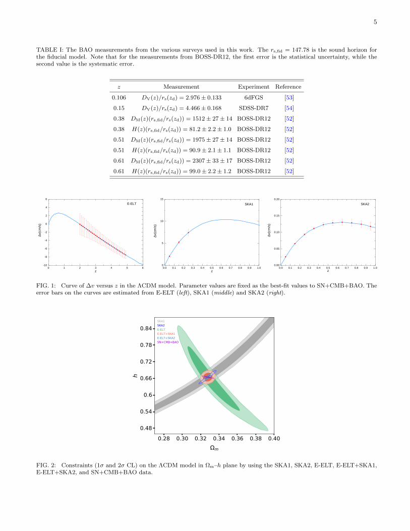
Since the ΛCDM model is widely regarded as a pro-totype of the standard cosmology, we take this model asa reference model to test the constraining power of theSKA-only mock data and make an analysis of constraintson cosmological parameters when the redshift drift dataof SKA and E-ELT are combined. In Fig. 1, we showthe simulated redshift-drift data for E-ELT, SKA1, andSKA2, using the ΛCDM model as the fiducial model.In this figure, the curve of ∆v(z) is plotted accordingto Eq. (23), with the fiducial values of parameters givenby the best fit to the SN+CMB+BAO data; the errorbars on ∆v, i.e., σ∆v, for each redshift bin, are plottedaccording to Eq. (24) for E-ELT, and according to thedetailed prescriptions described in the above section (thepart entitled “SKA mock data”) for SKA1 and SKA2.We find that in the E-ELT case the error of ∆v de-creases with the increase of redshift, and vice versa in

5

TABLE I: The BAO measurements from the various surveys used in this work. The rs,fid = 147.78 is the sound horizon forthe fiducial model. Note that for the measurements from BOSS-DR12, the first error is the statistical uncertainty, while thesecond value is the systematic error.

z Measurement Experiment Reference

0.106 DV(z)/rs(zd) = 2.976 ± 0.133 6dFGS [53]

0.15 DV(z)/rs(zd) = 4.466 ± 0.168 SDSS-DR7 [54]

0.38 DM(z)(rs,fid/rs(zd)) = 1512 ± 27 ± 14 BOSS-DR12 [52]

0.38 H(z)(rs,fid/rs(zd)) = 81.2 ± 2.2 ± 1.0 BOSS-DR12 [52]

0.51 DM(z)(rs,fid/rs(zd)) = 1975 ± 27 ± 14 BOSS-DR12 [52]

0.51 H(z)(rs,fid/rs(zd)) = 90.9 ± 2.1 ± 1.1 BOSS-DR12 [52]

0.61 DM(z)(rs,fid/rs(zd)) = 2307 ± 33 ± 17 BOSS-DR12 [52]

0.61 H(z)(rs,fid/rs(zd)) = 99.0 ± 2.2 ± 1.2 BOSS-DR12 [52]

0 1 2 3 4 5 6- 1 0

- 8

- 6

- 4

- 2

0

2

4

6

0 . 0 0 . 1 0 . 2 0 . 3 0 . 4 0 . 5 0 . 6 0 . 7 0 . 8 0 . 9 1 . 00

5

1 0

1 5

0 . 0 0 . 1 0 . 2 0 . 3 0 . 4 0 . 5 0 . 6 0 . 7 0 . 8 0 . 9 1 . 00 . 0 0

0 . 0 5

0 . 1 0

0 . 1 5

0 . 2 0E - E L T

∆v(cm

/s)

z

∆v(cm

/s)

z

S K A 1 S K A 2

∆v(cm

/s)z

FIG. 1: Curve of ∆v versus z in the ΛCDM model. Parameter values are fixed as the best-fit values to SN+CMB+BAO. Theerror bars on the curves are estimated from E-ELT (left), SKA1 (middle) and SKA2 (right).

0.28 0.30 0.32 0.34 0.36 0.38 0.40m

0.48

0.54

0.6

0.66

0.72

0.78

0.84

h

SKA1 SKA2E-ELTE-ELT+SKA1E-ELT+SKA2SN+CMB+BAO

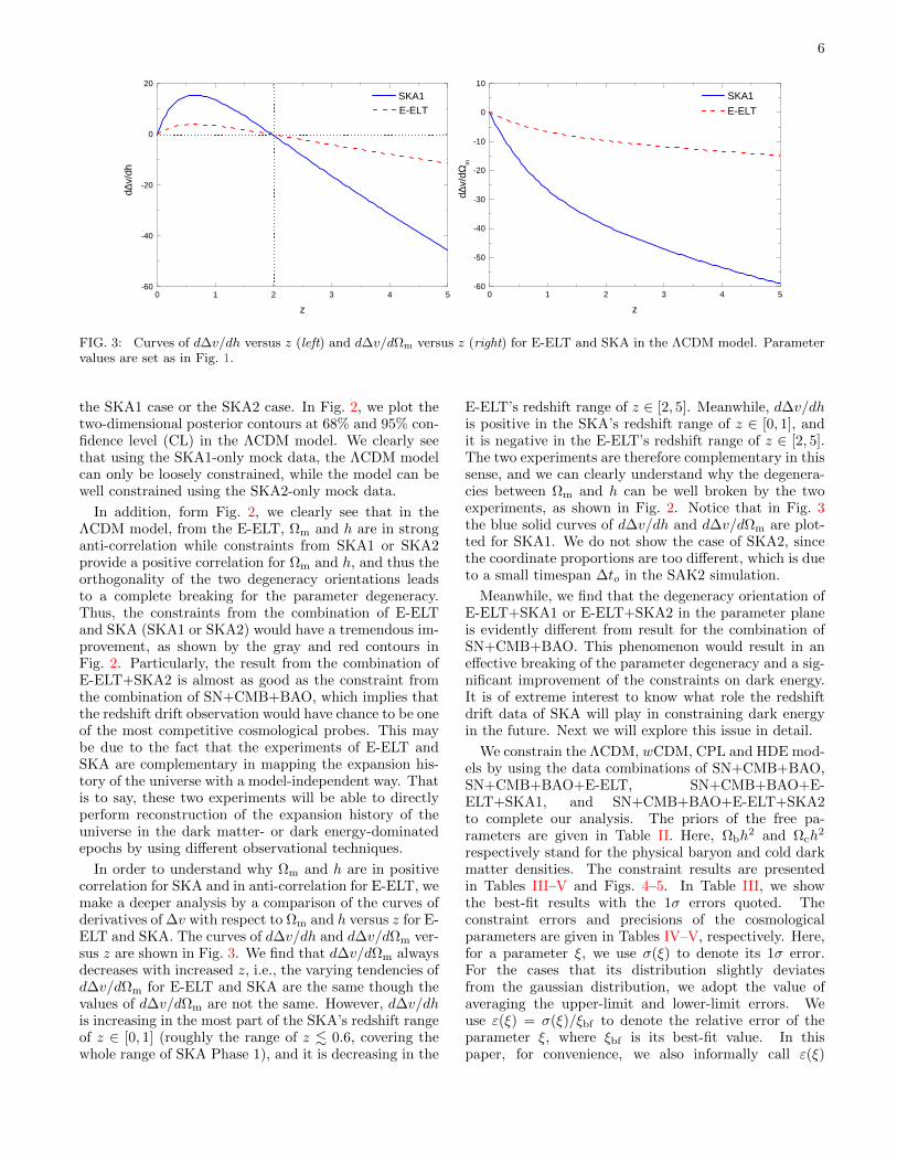
FIG. 2: Constraints (1σ and 2σ CL) on the ΛCDM model in Ωm–h plane by using the SKA1, SKA2, E-ELT, E-ELT+SKA1,E-ELT+SKA2, and SN+CMB+BAO data.

6

0 1 2 3 4 5- 6 0

- 4 0

- 2 0

0

2 0

0 1 2 3 4 5- 6 0

- 5 0

- 4 0

- 3 0

- 2 0

- 1 0

0

1 0

d∆v/d

h

z

S K A 1 E - E L T

d∆v/d

Ωm

z

S K A 1 E - E L T

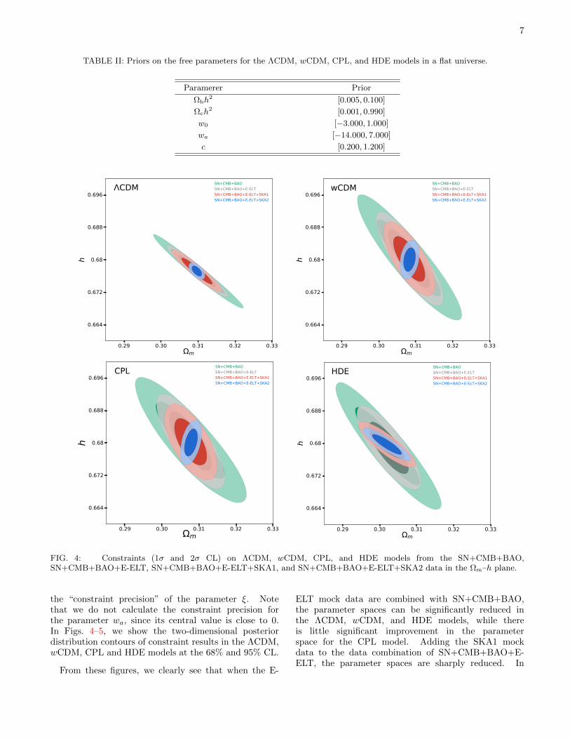
FIG. 3: Curves of d∆v/dh versus z (left) and d∆v/dΩm versus z (right) for E-ELT and SKA in the ΛCDM model. Parametervalues are set as in Fig. 1.

the SKA1 case or the SKA2 case. In Fig. 2, we plot thetwo-dimensional posterior contours at 68% and 95% con-fidence level (CL) in the ΛCDM model. We clearly seethat using the SKA1-only mock data, the ΛCDM modelcan only be loosely constrained, while the model can bewell constrained using the SKA2-only mock data.

In addition, form Fig. 2, we clearly see that in theΛCDM model, from the E-ELT, Ωm and h are in stronganti-correlation while constraints from SKA1 or SKA2provide a positive correlation for Ωm and h, and thus theorthogonality of the two degeneracy orientations leadsto a complete breaking for the parameter degeneracy.Thus, the constraints from the combination of E-ELTand SKA (SKA1 or SKA2) would have a tremendous im-provement, as shown by the gray and red contours inFig. 2. Particularly, the result from the combination ofE-ELT+SKA2 is almost as good as the constraint fromthe combination of SN+CMB+BAO, which implies thatthe redshift drift observation would have chance to be oneof the most competitive cosmological probes. This maybe due to the fact that the experiments of E-ELT andSKA are complementary in mapping the expansion his-tory of the universe with a model-independent way. Thatis to say, these two experiments will be able to directlyperform reconstruction of the expansion history of theuniverse in the dark matter- or dark energy-dominatedepochs by using different observational techniques.

In order to understand why Ωm and h are in positivecorrelation for SKA and in anti-correlation for E-ELT, wemake a deeper analysis by a comparison of the curves ofderivatives of ∆v with respect to Ωm and h versus z for E-ELT and SKA. The curves of d∆v/dh and d∆v/dΩm ver-sus z are shown in Fig. 3. We find that d∆v/dΩm alwaysdecreases with increased z, i.e., the varying tendencies ofd∆v/dΩm for E-ELT and SKA are the same though thevalues of d∆v/dΩm are not the same. However, d∆v/dhis increasing in the most part of the SKA’s redshift rangeof z ∈ [0, 1] (roughly the range of z . 0.6, covering thewhole range of SKA Phase 1), and it is decreasing in the

E-ELT’s redshift range of z ∈ [2, 5]. Meanwhile, d∆v/dhis positive in the SKA’s redshift range of z ∈ [0, 1], andit is negative in the E-ELT’s redshift range of z ∈ [2, 5].The two experiments are therefore complementary in thissense, and we can clearly understand why the degenera-cies between Ωm and h can be well broken by the twoexperiments, as shown in Fig. 2. Notice that in Fig. 3the blue solid curves of d∆v/dh and d∆v/dΩm are plot-ted for SKA1. We do not show the case of SKA2, sincethe coordinate proportions are too different, which is dueto a small timespan ∆to in the SAK2 simulation.

Meanwhile, we find that the degeneracy orientation ofE-ELT+SKA1 or E-ELT+SKA2 in the parameter planeis evidently different from result for the combination ofSN+CMB+BAO. This phenomenon would result in aneffective breaking of the parameter degeneracy and a sig-nificant improvement of the constraints on dark energy.It is of extreme interest to know what role the redshiftdrift data of SKA will play in constraining dark energyin the future. Next we will explore this issue in detail.

We constrain the ΛCDM, wCDM, CPL and HDE mod-els by using the data combinations of SN+CMB+BAO,SN+CMB+BAO+E-ELT, SN+CMB+BAO+E-ELT+SKA1, and SN+CMB+BAO+E-ELT+SKA2to complete our analysis. The priors of the free pa-rameters are given in Table II. Here, Ωbh

2 and Ωch2

respectively stand for the physical baryon and cold darkmatter densities. The constraint results are presentedin Tables III–V and Figs. 4–5. In Table III, we showthe best-fit results with the 1σ errors quoted. Theconstraint errors and precisions of the cosmologicalparameters are given in Tables IV–V, respectively. Here,for a parameter ξ, we use σ(ξ) to denote its 1σ error.For the cases that its distribution slightly deviatesfrom the gaussian distribution, we adopt the value ofaveraging the upper-limit and lower-limit errors. Weuse ε(ξ) = σ(ξ)/ξbf to denote the relative error of theparameter ξ, where ξbf is its best-fit value. In thispaper, for convenience, we also informally call ε(ξ)

7

TABLE II: Priors on the free parameters for the ΛCDM, wCDM, CPL, and HDE models in a flat universe.

Paramerer Prior

Ωbh2 [0.005, 0.100]

Ωch2 [0.001, 0.990]

w0 [−3.000, 1.000]

wa [−14.000, 7.000]

c [0.200, 1.200]

0.29 0.30 0.31 0.32 0.33m

0.664

0.672

0.68

0.688

0.696

h

CDM SN+CMB+BAOSN+CMB+BAO+E-ELTSN+CMB+BAO+E-ELT+SKA1SN+CMB+BAO+E-ELT+SKA2

0.29 0.30 0.31 0.32 0.33m

0.664

0.672

0.68

0.688

0.696

h

wCDM SN+CMB+BAOSN+CMB+BAO+E-ELTSN+CMB+BAO+E-ELT+SKA1SN+CMB+BAO+E-ELT+SKA2

0.29 0.30 0.31 0.32 0.33m

0.664

0.672

0.68

0.688

0.696

h

CPL SN+CMB+BAOSN+CMB+BAO+E-ELTSN+CMB+BAO+E-ELT+SKA1SN+CMB+BAO+E-ELT+SKA2

0.29 0.30 0.31 0.32 0.33m

0.664

0.672

0.68

0.688

0.696

h

HDE SN+CMB+BAOSN+CMB+BAO+E-ELTSN+CMB+BAO+E-ELT+SKA1SN+CMB+BAO+E-ELT+SKA2

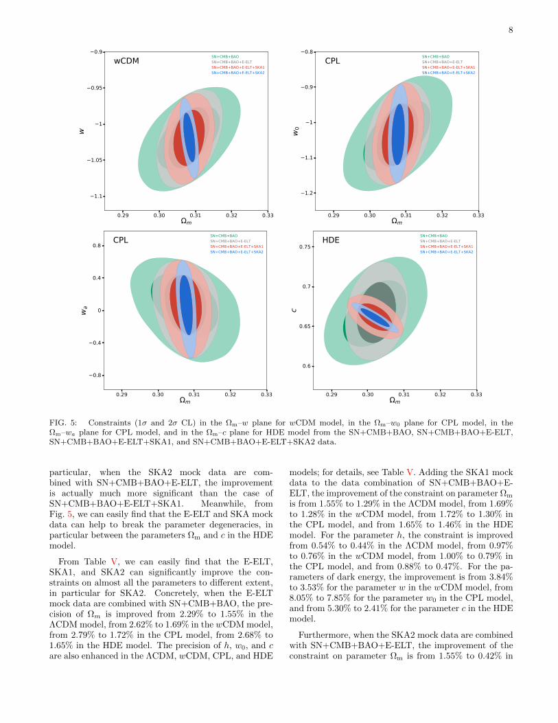
FIG. 4: Constraints (1σ and 2σ CL) on ΛCDM, wCDM, CPL, and HDE models from the SN+CMB+BAO,SN+CMB+BAO+E-ELT, SN+CMB+BAO+E-ELT+SKA1, and SN+CMB+BAO+E-ELT+SKA2 data in the Ωm–h plane.

the “constraint precision” of the parameter ξ. Notethat we do not calculate the constraint precision forthe parameter wa, since its central value is close to 0.In Figs. 4–5, we show the two-dimensional posteriordistribution contours of constraint results in the ΛCDM,wCDM, CPL and HDE models at the 68% and 95% CL.

From these figures, we clearly see that when the E-

ELT mock data are combined with SN+CMB+BAO,the parameter spaces can be significantly reduced inthe ΛCDM, wCDM, and HDE models, while thereis little significant improvement in the parameterspace for the CPL model. Adding the SKA1 mockdata to the data combination of SN+CMB+BAO+E-ELT, the parameter spaces are sharply reduced. In

8

0.29 0.30 0.31 0.32 0.33m

1.1

1.05

1

0.95

0.9

w

wCDM SN+CMB+BAOSN+CMB+BAO+E-ELTSN+CMB+BAO+E-ELT+SKA1SN+CMB+BAO+E-ELT+SKA2

0.29 0.30 0.31 0.32 0.33m

1.2

1.1

1

0.9

0.8

w0

CPL SN+CMB+BAOSN+CMB+BAO+E-ELTSN+CMB+BAO+E-ELT+SKA1SN+CMB+BAO+E-ELT+SKA2

0.29 0.30 0.31 0.32 0.33m

0.8

0.4

0

0.4

0.8

wa

CPL SN+CMB+BAOSN+CMB+BAO+E-ELTSN+CMB+BAO+E-ELT+SKA1SN+CMB+BAO+E-ELT+SKA2

0.29 0.30 0.31 0.32 0.33m

0.6

0.65

0.7

0.75

c

HDE SN+CMB+BAOSN+CMB+BAO+E-ELTSN+CMB+BAO+E-ELT+SKA1SN+CMB+BAO+E-ELT+SKA2

FIG. 5: Constraints (1σ and 2σ CL) in the Ωm–w plane for wCDM model, in the Ωm–w0 plane for CPL model, in theΩm–wa plane for CPL model, and in the Ωm–c plane for HDE model from the SN+CMB+BAO, SN+CMB+BAO+E-ELT,SN+CMB+BAO+E-ELT+SKA1, and SN+CMB+BAO+E-ELT+SKA2 data.

particular, when the SKA2 mock data are com-bined with SN+CMB+BAO+E-ELT, the improvementis actually much more significant than the case ofSN+CMB+BAO+E-ELT+SKA1. Meanwhile, fromFig. 5, we can easily find that the E-ELT and SKA mockdata can help to break the parameter degeneracies, inparticular between the parameters Ωm and c in the HDEmodel.

From Table V, we can easily find that the E-ELT,SKA1, and SKA2 can significantly improve the con-straints on almost all the parameters to different extent,in particular for SKA2. Concretely, when the E-ELTmock data are combined with SN+CMB+BAO, the pre-cision of Ωm is improved from 2.29% to 1.55% in theΛCDM model, from 2.62% to 1.69% in the wCDM model,from 2.79% to 1.72% in the CPL model, from 2.68% to1.65% in the HDE model. The precision of h, w0, and care also enhanced in the ΛCDM, wCDM, CPL, and HDE

models; for details, see Table V. Adding the SKA1 mockdata to the data combination of SN+CMB+BAO+E-ELT, the improvement of the constraint on parameter Ωm

is from 1.55% to 1.29% in the ΛCDM model, from 1.69%to 1.28% in the wCDM model, from 1.72% to 1.30% inthe CPL model, and from 1.65% to 1.46% in the HDEmodel. For the parameter h, the constraint is improvedfrom 0.54% to 0.44% in the ΛCDM model, from 0.97%to 0.76% in the wCDM model, from 1.00% to 0.79% inthe CPL model, and from 0.88% to 0.47%. For the pa-rameters of dark energy, the improvement is from 3.84%to 3.53% for the parameter w in the wCDM model, from8.05% to 7.85% for the parameter w0 in the CPL model,and from 5.30% to 2.41% for the parameter c in the HDEmodel.

Furthermore, when the SKA2 mock data are combinedwith SN+CMB+BAO+E-ELT, the improvement of theconstraint on parameter Ωm is from 1.55% to 0.42% in

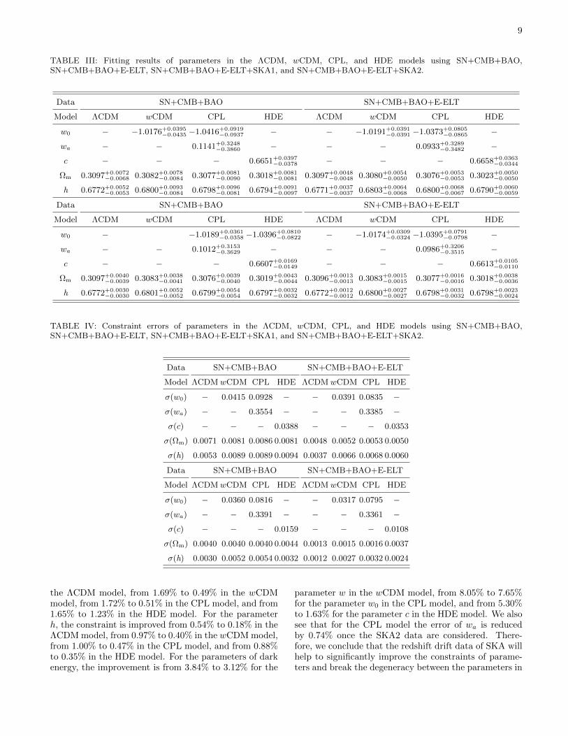
9

TABLE III: Fitting results of parameters in the ΛCDM, wCDM, CPL, and HDE models using SN+CMB+BAO,SN+CMB+BAO+E-ELT, SN+CMB+BAO+E-ELT+SKA1, and SN+CMB+BAO+E-ELT+SKA2.

Data SN+CMB+BAO SN+CMB+BAO+E-ELT

Model ΛCDM wCDM CPL HDE ΛCDM wCDM CPL HDE

w0 − −1.0176+0.0395−0.0435 −1.0416+0.0919

−0.0937 − − −1.0191+0.0391−0.0391 −1.0373+0.0805

−0.0865 −

wa − − 0.1141+0.3248−0.3860 − − − 0.0933+0.3289

−0.3482 −

c − − − 0.6651+0.0397−0.0378 − − − 0.6658+0.0363

−0.0344

Ωm 0.3097+0.0072−0.0068 0.3082+0.0078

−0.0084 0.3077+0.0081−0.0090 0.3018+0.0081

−0.0081 0.3097+0.0048−0.0048 0.3080+0.0054

−0.0050 0.3076+0.0053−0.0053 0.3023+0.0050

−0.0050

h 0.6772+0.0052−0.0053 0.6800+0.0093

−0.0084 0.6798+0.0096−0.0081 0.6794+0.0091

−0.0097 0.6771+0.0037−0.0037 0.6803+0.0064

−0.0068 0.6800+0.0068−0.0067 0.6790+0.0060

−0.0059

Data SN+CMB+BAO SN+CMB+BAO+E-ELT

Model ΛCDM wCDM CPL HDE ΛCDM wCDM CPL HDE

w0 − −1.0189+0.0361−0.0358 −1.0396+0.0810

−0.0822 − −1.0174+0.0309−0.0324 −1.0395+0.0791

−0.0798 −

wa − − 0.1012+0.3153−0.3629 − − − 0.0986+0.3206

−0.3515 −

c − − − 0.6607+0.0169−0.0149 − − − 0.6613+0.0105

−0.0110

Ωm 0.3097+0.0040−0.0039 0.3083+0.0038

−0.0041 0.3076+0.0039−0.0040 0.3019+0.0043

−0.0044 0.3096+0.0013−0.0013 0.3083+0.0015

−0.0015 0.3077+0.0016−0.0016 0.3018+0.0038

−0.0036

h 0.6772+0.0030−0.0030 0.6801+0.0052

−0.0052 0.6799+0.0054−0.0054 0.6797+0.0032

−0.0032 0.6772+0.0012−0.0012 0.6800+0.0027

−0.0027 0.6798+0.0031−0.0032 0.6798+0.0023

−0.0024

TABLE IV: Constraint errors of parameters in the ΛCDM, wCDM, CPL, and HDE models using SN+CMB+BAO,SN+CMB+BAO+E-ELT, SN+CMB+BAO+E-ELT+SKA1, and SN+CMB+BAO+E-ELT+SKA2.

Data SN+CMB+BAO SN+CMB+BAO+E-ELT

Model ΛCDM wCDM CPL HDE ΛCDM wCDM CPL HDE

σ(w0) − 0.0415 0.0928 − − 0.0391 0.0835 −

σ(wa) − − 0.3554 − − − 0.3385 −

σ(c) − − − 0.0388 − − − 0.0353

σ(Ωm) 0.0071 0.0081 0.0086 0.0081 0.0048 0.0052 0.0053 0.0050

σ(h) 0.0053 0.0089 0.0089 0.0094 0.0037 0.0066 0.0068 0.0060

Data SN+CMB+BAO SN+CMB+BAO+E-ELT

Model ΛCDM wCDM CPL HDE ΛCDM wCDM CPL HDE

σ(w0) − 0.0360 0.0816 − − 0.0317 0.0795 −

σ(wa) − − 0.3391 − − − 0.3361 −

σ(c) − − − 0.0159 − − − 0.0108

σ(Ωm) 0.0040 0.0040 0.0040 0.0044 0.0013 0.0015 0.0016 0.0037

σ(h) 0.0030 0.0052 0.0054 0.0032 0.0012 0.0027 0.0032 0.0024

the ΛCDM model, from 1.69% to 0.49% in the wCDMmodel, from 1.72% to 0.51% in the CPL model, and from1.65% to 1.23% in the HDE model. For the parameterh, the constraint is improved from 0.54% to 0.18% in theΛCDM model, from 0.97% to 0.40% in the wCDM model,from 1.00% to 0.47% in the CPL model, and from 0.88%to 0.35% in the HDE model. For the parameters of darkenergy, the improvement is from 3.84% to 3.12% for the

parameter w in the wCDM model, from 8.05% to 7.65%for the parameter w0 in the CPL model, and from 5.30%to 1.63% for the parameter c in the HDE model. We alsosee that for the CPL model the error of wa is reducedby 0.74% once the SKA2 data are considered. There-fore, we conclude that the redshift drift data of SKA willhelp to significantly improve the constraints of parame-ters and break the degeneracy between the parameters in

10

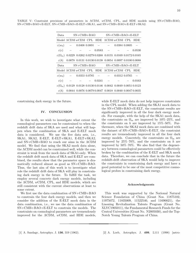
TABLE V: Constraint precisions of parameters in ΛCDM, wCDM, CPL, and HDE models using SN+CMB+BAO,SN+CMB+BAO+E-ELT, SN+CMB+BAO+E-ELT+SKA1, and SN+CMB+BAO+E-ELT+SKA2.

Data SN+CMB+BAO SN+CMB+BAO+E-ELT

Model ΛCDM wCDM CPL HDE ΛCDM wCDM CPL HDE

ε(w0) − 0.0408 0.0891 − − 0.0384 0.0805 −

ε(c) − − − 0.0583 − − − 0.0530

ε(Ωm) 0.0229 0.0262 0.0279 0.0268 0.0155 0.0169 0.0172 0.0165

ε(h) 0.0078 0.0131 0.0130 0.0138 0.0054 0.0097 0.0100 0.0088

Data SN+CMB+BAO SN+CMB+BAO+E-ELT

Model ΛCDM wCDM CPL HDE ΛCDM wCDM CPL HDE

ε(w0) − 0.0353 0.0785 − − 0.0312 0.0765 −

ε(c) − − − 0.0241 − − − 0.0163

ε(Ωm) 0.0129 0.0128 0.0130 0.0146 0.0042 0.0049 0.0051 0.0123

ε(h) 0.0044 0.0076 0.0079 0.0047 0.0018 0.0040 0.0047 0.0035

constraining dark energy in the future.

IV. CONCLUSION

In this work, we wish to investigate what extent thecosmological parameters can be constrained to when theredshift drift data of SKA are used and what will hap-pen when the combination of SKA and E-ELT mockdata is considered. We use the five data sets, i.e.,SKA1, SKA2, E-ELT, E-ELT+SKA1, E-ELT+SKA2,and SN+CMB+BAO to reach our aims in the ΛCDMmodel. We find that using the SKA2 mock data alone,the ΛCDM model can be constrained well, while the con-straint is weak from the mock data of SKA1-only. Whenthe redshift drift mock data of SKA and E-ELT are com-bined, the results show that the parameter space is dra-matically reduced almost as good as SN+CMB+BAO.Thus, the last aim of this work is to investigate whatrole the redshift drift data of SKA will play in constrain-ing dark energy in the future. To fulfill the task, weemploy several concrete dark energy models, includingthe ΛCDM, wCDM, CPL, and HDE models, which arestill consistent with the current observations at least tosome extent.

We first use the data combination of SN+CMB+BAOto constrain the four dark energy models, and then weconsider the addition of the E-ELT mock data in thedata combination, i.e., we use the data combination ofSN+CMB+BAO+E-ELT to constrain the models. Theconstraints on cosmological parameters are tremendouslyimproved for the ΛCDM, wCDM, and HDE models,

while E-ELT mock data do not help improve constraintsin the CPL model. When adding the SKA1 mock data tothe SN+CMB+BAO+E-ELT, the constraint results aresignificantly improved in all the four dark energy mod-els. For example, with the help of the SKA1 mock data,the constraints on Ωm are improved by 10%–25%, andthe constraints on h are improved by 15%–50%. Fur-thermore, when the SKA2 mock data are combined withthe dataset of SN+CMB+BAO+E-ELT, the constraintresults are tremendously improved in all the four darkenergy models. Concretely, the constraints on Ωm areimproved by 25%–70%, and the constraints on h areimproved by 50%–70%. We also find that the degener-acy between cosmological parameters could be effectivelybroken by the combination of the E-ELT and SKA mockdata. Therefore, we can conclude that in the future theredshift-drift observation of SKA would help to improvethe constraints in constraining dark energy and have agood potential to be one of the most competitive cosmo-logical probes in constraining dark energy.

Acknowledgments

This work was supported by the National NaturalScience Foundation of China (Grant Nos. 11875102,11975072, 11835009, 11522540, and 11690021), theLiaoning Revitalization Talents Program (Grant No.XLYC1905011), the Fundamental Research Funds for theCentral Universities (Grant No. N2005030), and the Top-Notch Young Talents Program of China.

[1] A. Sandage, Astrophys. J. 136, 319 (1962). [2] A. Loeb, Astrophys. J. 499, L111 (1998) [astro-

11

ph/9802122].[3] H. B. Zhang, W. H. Zhong, Z. H. Zhu and S. He, Phys.

Rev. D 76, 123508 (2007) [arXiv:0705.4409 [astro-ph]].[4] P. S. Corasaniti, D. Huterer and A. Melchiorri, Phys.

Rev. D 75, 062001 (2007) [astro-ph/0701433].[5] A. Balbi and C. Quercellini, Mon. Not. R. Astron. Soc.

382, 1623 (2007) [arXiv:0704.2350 [astro-ph]].[6] J. Liske et al., Mon. Not. Roy. Astron. Soc. 386, 1192

(2008) [arXiv:0802.1532 [astro-ph]].[7] J. Zhang, L. Zhang and X. Zhang, Phys. Lett. B 691, 11

(2010) [arXiv:1006.1738 [astro-ph.CO]].[8] M. Martinelli et al., Phys. Rev. D 86, 123001 (2012)

[arXiv:1210.7166 [astro-ph.CO]].[9] S. Yuan and T. J. Zhang, JCAP 1502, no. 02, 025 (2015)

[arXiv:1311.1583 [astro-ph.CO]].[10] M. J. Zhang and W. B. Liu, arXiv:1311.6858 [astro-

ph.CO].[11] J. J. Geng, J. F. Zhang and X. Zhang, JCAP 1407, 006

(2014) [arXiv:1404.5407 [astro-ph.CO]].[12] J. J. Geng, J. F. Zhang and X. Zhang, JCAP 1412, no.

12, 018 (2014) [arXiv:1407.7123 [astro-ph.CO]].[13] J. J. Geng, Y. H. Li, J. F. Zhang and X. Zhang, Eur.

Phys. J. C 75, no. 8, 356 (2015) [arXiv:1501.03874 [astro-ph.CO]].

[14] R. Y. Guo and X. Zhang, Eur. Phys. J. C 76, no. 3, 163(2016) [arXiv:1512.07703 [astro-ph.CO]].

[15] D. Z. He, J. F. Zhang and X. Zhang, Sci.China Phys. Mech. Astron. 60 (2017) no.3, 039511doi:10.1007/s11433-016-0472-1 [arXiv:1607.05643 [astro-ph.CO]].

[16] R. Lazkoz, I. Leanizbarrutia and V. Salzano, Eur. Phys.J. C 78, no. 1, 11 (2018) [arXiv:1712.07555 [astro-ph.CO]].

[17] J. J. Geng, R. Y. Guo, A. Wang, J. F. Zhang andX. Zhang, Commun. Theor. Phys. 70, no. 4, 445 (2018)[arXiv:1806.10735 [astro-ph.CO]].

[18] Y. Liu, R. Y. Guo, J. F. Zhang and X. Zhang, JCAP1905, 016 (2019) [arXiv:1811.12131 [astro-ph.CO]].

[19] M. Chevallier and D. Polarski, Int. J. Mod. Phys. D 10,213 (2001) [gr-qc/0009008].

[20] E. V. Linder, Phys. Rev. Lett. 90, 091301 (2003) [astro-ph/0208512].

[21] A. G. Cohen, D. B. Kaplan and A. E. Nelson, Phys. Rev.Lett. 82, 4971 (1999) [hep-th/9803132].

[22] M. Li, Phys. Lett. B 603, 1 (2004) [hep-th/0403127].[23] X. Zhang, Int. J. Mod. Phys. D 14, 1597 (2005) [astro-

ph/0504586].[24] X. Zhang and F. Q. Wu, Phys. Rev. D 72, 043524 (2005)

[astro-ph/0506310].[25] X. Zhang, Phys. Rev. D 74, 103505 (2006)

doi:10.1103/PhysRevD.74.103505 [astro-ph/0609699].[26] X. Zhang, Phys. Lett. B 648, 1 (2007)

doi:10.1016/j.physletb.2007.02.069 [astro-ph/0604484].[27] X. Zhang and F. Q. Wu, Phys. Rev. D 76, 023502 (2007)

[astro-ph/0701405].[28] J. Zhang, X. Zhang and H. Liu, Phys. Lett.

B 651, 84 (2007) doi:10.1016/j.physletb.2007.06.019[arXiv:0706.1185 [astro-ph]].

[29] J. f. Zhang, X. Zhang and H. y. Liu, Eur. Phys. J.C 52, 693 (2007) doi:10.1140/epjc/s10052-007-0408-2[arXiv:0708.3121 [hep-th]].

[30] J. F. Zhang, X. Zhang and H. Liu, Eur. Phys. J.C 54, 303 (2008) doi:10.1140/epjc/s10052-008-0532-7[arXiv:0801.2809 [astro-ph]].

[31] C. Gao, F. Wu, X. Chen and Y. G. Shen, Phys. Rev. D79, 043511 (2009) [arXiv:0712.1394 [astro-ph]].

[32] M. Li, X. D. Li, S. Wang and X. Zhang, JCAP 0906,036 (2009) [arXiv:0904.0928 [astro-ph.CO]].

[33] X. Zhang, Phys. Rev. D 79, 103509 (2009)doi:10.1103/PhysRevD.79.103509 [arXiv:0901.2262[astro-ph.CO]].

[34] C. J. Feng and X. Zhang, Phys. Lett. B 680, 399 (2009)doi:10.1016/j.physletb.2009.09.040 [arXiv:0904.0045 [gr-qc]].

[35] M. Li, X. Li and X. Zhang, Sci. China Phys. Mech. As-tron. 53, 1631 (2010) [arXiv:0912.3988 [astro-ph.CO]].

[36] J. L. Cui, L. Zhang, J. F. Zhang and X. Zhang,Chin. Phys. B 19, 019802 (2010) doi:10.1088/1674-1056/19/1/019802 [arXiv:0902.0716 [astro-ph.CO]].

[37] Y. H. Li, S. Wang, X. D. Li and X. Zhang, JCAP1302, 033 (2013) doi:10.1088/1475-7516/2013/02/033[arXiv:1207.6679 [astro-ph.CO]].

[38] J. F. Zhang, M. M. Zhao, J. L. Cui andX. Zhang, Eur. Phys. J. C 74, no. 11, 3178 (2014)doi:10.1140/epjc/s10052-014-3178-7 [arXiv:1409.6078[astro-ph.CO]].

[39] J. L. Cui and J. F. Zhang, Eur. Phys. J. C 74, 2849(2014) [arXiv:1402.1829 [astro-ph.CO]].

[40] J. F. Zhang, J. L. Cui and X. Zhang, Eur. Phys. J. C 74,no. 10, 3100 (2014) [arXiv:1409.6562 [astro-ph.CO]].

[41] J. F. Zhang, M. M. Zhao, Y. H. Li and X. Zhang, JCAP1504, 038 (2015) doi:10.1088/1475-7516/2015/04/038[arXiv:1502.04028 [astro-ph.CO]].

[42] X. Zhang, Phys. Rev. D 93, no. 8, 083011 (2016)doi:10.1103/PhysRevD.93.083011 [arXiv:1511.02651[astro-ph.CO]].

[43] S. Wang, Y. F. Wang, D. M. Xia and X. Zhang,Phys. Rev. D 94, no. 8, 083519 (2016)doi:10.1103/PhysRevD.94.083519 [arXiv:1608.00672[astro-ph.CO]].

[44] M. M. Zhao, D. Z. He, J. F. Zhang andX. Zhang, Phys. Rev. D 96, no. 4, 043520 (2017)doi:10.1103/PhysRevD.96.043520 [arXiv:1703.08456[astro-ph.CO]].

[45] L. Feng, Y. H. Li, F. Yu, J. F. Zhang andX. Zhang, Eur. Phys. J. C 78, no. 10, 865 (2018)doi:10.1140/epjc/s10052-018-6338-3 [arXiv:1807.03022[astro-ph.CO]].

[46] J. F. Zhang, H. Y. Dong, J. Z. Qi and X. Zhang,arXiv:1906.07504 [astro-ph.CO].

[47] D. M. Scolnic et al., Astrophys. J. 859, no. 2, 101 (2018)[arXiv:1710.00845 [astro-ph.CO]].

[48] R. Tripp, A&A 331, 815 (1998)[49] SNLS Collaboration (J. Guy et al.) A&A 523 (2010) A7

[arXiv:1010.4743[astro-ph.CO]][50] P. A. R. Ade et al. [Planck Collaboration], Astron. Astro-

phys. 594, A14 (2016) [arXiv:1502.01590 [astro-ph.CO]].[51] W. Hu and N. Sugiyama, Astrophys. J. 471, 542 (1996)

[astro-ph/9510117].[52] S. Alam et al. [BOSS Collaboration], Mon. Not. Roy.

Astron. Soc. 470, no. 3, 2617 (2017) [arXiv:1607.03155[astro-ph.CO]].

[53] F. Beutler et al., Mon. Not. Roy. Astron. Soc. 416, 3017(2011) [arXiv:1106.3366 [astro-ph.CO]].

[54] A. J. Ross, L. Samushia, C. Howlett, W. J. Percival,A. Burden and M. Manera, Mon. Not. Roy. Astron. Soc.449, no. 1, 835 (2015) [arXiv:1409.3242 [astro-ph.CO]].

[55] J. Liske et al., Top Level Requirements For ELT-HIRES,

12

Document ESO 204697 Version 1 (2014).[56] H. R. Klckner et al., PoS AASKA 14, 027 (2015)

[arXiv:1501.03822 [astro-ph.CO]].[57] C. J. A. P. Martins, M. Martinelli, E. Calabrese and

M. P. L. P. Ramos, Phys. Rev. D 94, no. 4, 043001 (2016)[arXiv:1606.07261 [astro-ph.CO]].

[58] N. Aghanim et al. [Planck Collaboration],arXiv:1807.06209 [astro-ph.CO].

[59] Y. Y. Xu and X. Zhang, Eur. Phys. J. C 76, no. 11, 588(2016) [arXiv:1607.06262 [astro-ph.CO]].