Real-Time Cloud Simulation and Rendering

byMark Jason Harris

A dissertation submitted to the faculty of the University of North Carolina at ChapelHill in partial fulfillment of the requirements for the degree of Doctor of Philosophy inthe Department of Computer Science.

Chapel Hill2003

Approved by:

Anselmo Lastra, Advisor

Gary Bishop, Reader

Ming C. Lin, Reader

David Leith, Reader

Frederick P. Brooks, Jr., Committee Member

ii

iii

c© 2003

Mark Jason Harris

ALL RIGHTS RESERVED

iv

v

ABSTRACTMARK JASON HARRIS: Real-Time Cloud Simulation and Rendering.

(Under the direction of Anselmo Lastra.)

Clouds are a ubiquitous, awe-inspiring, and ever-changing feature of the outdoors.

They are an integral factor in Earth’s weather systems, and a strong indicator of weather

patterns and changes. Their effects and indications are important to flight and flight

training. Clouds are an important component of the visual simulation of any outdoor

scene, but the complexity of cloud formation, dynamics, and light interaction makes

cloud simulation and rendering difficult in real time. In an interactive flight simulation,

users would like to fly in and around realistic, volumetric clouds, and to see other aircraft

convincingly pass within and behind them. Ideally, simulated clouds would grow and

disperse as real clouds do, and move in response to wind and other forces. Simulated

clouds should be realistically illuminated by direct sunlight, internal scattering, and

reflections from the sky and the earth below. Previous real-time techniques have not

provided users with such experiences.

I present a physically-based, visually-realistic cloud simulation suitable for inter-

active applications such as flight simulators. Clouds in the system are modeled us-

ing partial differential equations describing fluid motion, thermodynamic processes,

buoyant forces, and water phase transitions. I also simulate the interaction of clouds

with light, including self-shadowing and multiple forward light scattering. I implement

both simulations—dynamic and radiometric—entirely on programmable floating point

graphics hardware. The speed and parallelism of graphics hardware enables simulation

of cloud dynamics in real time. I exploit the relatively slow evolution of clouds in calm

skies to enable interactive visualization of the simulation. The work required to simu-

late a single time step is automatically spread over many frames while the user views

the results of the previous time step. I use dynamically-generated impostors to ac-

celerate cloud rendering. These techniques enable incorporation of realistic, simulated

clouds into real applications without sacrificing interactivity.

Beyond clouds, I also present general techniques for using graphics hardware to sim-

ulate dynamic phenomena ranging from fluid dynamics to chemical reaction-diffusion.

I demonstrate that these simulations can be executed faster on graphics hardware than

on traditional CPUs.

vi

vii

ACKNOWLEDGMENTS

I would like to thank Anselmo Lastra, who is always available and attentive, and has

patiently guided me through the steps of my Ph.D. I thank him for being a great

advisor, teacher, and friend. Anselmo convinced me that my initial work on clouds

was a good start at a Ph.D. topic. Without his honest encouragement I may have left

graduate school much earlier.

I thank my committee—Professors Fred Brooks, Gary Bishop, David Leith, Ming

Lin, and Parker Reist—for their feedback and for many enlightening discussions. I

thank Parker Reist for many interesting conversations about clouds and light scattering,

and David Leith for later filling in for Professor Reist. I also thank Dinesh Manocha for

his guidance, especially during my first year at UNC as part of the Walkthrough Group.

I would not have completed this work without Fred Brooks, Mary Whitton, and the

Effective Virtual Environments group, who were kind enough to let me “wildcat” with

research outside of the group’s primary focus.

I began working on cloud rendering at iROCK Games during an internship in the

summer and fall of 2000. Robert Stevenson gave me the task of creating realistic,

volumetric clouds for the game Savage Skies (iROCK Games, 2002). I thank Robert

and the others who helped me at iROCK, including Brian Stone, Wesley Hunt, and

Paul Rowan.

NVIDIA Corporation has given me wonderful help and support over the past two

years, starting with an internship in the Developer Technology group during the summer

of 2001, followed by two years of fellowship support. I also thank everyone from NVIDIA

who provided help, especially John Spitzer, David Kirk, Steve Molnar, Chris Wynn,

Sebastien Domine, Greg James, Cass Everritt, Ashu Rege, Simon Green, Jason Allen,

Jeff Juliano, Stephen Ehmann, Pat Brown, Mike Bunnell, Randy Fernando, and Chris

Seitz. Also, Section 4.2, which will appear as an article in (Fernando, 2004), was edited

by Randy Fernando, Simon Green, and Catherine Kilkenny, and Figures 4.2, 4.3, 4.4,

4.5, and 4.6 were drawn by Spender Yuen.

viii

Discussions with researchers outside of UNC have been enlightening. I have enjoyed

conversations about general purpose computation on GPUs with Nolan Goodnight,

Cliff Woolley, and Dave Luebke of the University of Virginia, Aaron Lefohn of the

University of Utah, and Tim Purcell of Stanford University. Recently, Kirk Riley of

Purdue University helped me with scattering phase function data and the MiePlot

software (Laven, 2003).

I am especially thankful for my fellow students. On top of being great friends, they

have been a constant source of encouragement and creative ideas. Rui Bastos gave me

help with global illumination as well as general guidance over the years. Bill Baxter,

Greg Coombe, and Thorsten Scheuermann collaborated with me on two of the papers

that became parts of this dissertation. Some students were my teachers as much as

they were my classmates. I can always turn to Bill Baxter for help with fluid dynamics

and numerical methods. Wesley Hunt is an expert programmer and has been helpful

in answering many software engineering questions. Sharif Razzaque provides creative

insight with a side of goofiness.

Computer science graduate students at UNC would have a rough time without the

daily help of the staff of our department. I am grateful for the support of these people,

especially Janet Jones, David Harrison, Sandra Neely, Tim Quigg, Karen Thigpen, and

the department facilities staff.

The research reported in this dissertation was supported in parts by an NVIDIA Fel-

lowship and funding from iROCK Games, The Link Foundation, NIH National Center

for Research Resources grant P41 RR 02170, Department of Energy ASCI program, Na-

tional Science Foundation grants ACR-9876914, IIS-0121293, and ACI-0205425, Office

of Naval Research grant N00014-01-1-0061, and NIH National Institute of Biomedical

Imaging and Bioengineering grant P41 EB-002025.

My friends in Chapel Hill helped me maintain sanity during stressful times. Bill

Baxter, Mike Brown, Greg Coombe, Scott Cooper, Caroline Green, David Marshburn,

Samir Naik, Andrew Nashel, Chuck Pisula, Sharif Razzaque, Stefan Sain, Alicia Tribble,

Kelly Ward, and Andrew Zaferakis helped ensure that no matter how hard I worked, I

played just as hard.

Finally, I thank my parents, Jay and Virginia Harris, who inspire me with their

dedication, attention to detail, and ability to drop everything and go to the beach.

ix

Contents

List of Figures xiii

List of Tables xv

List of Abbreviations xvii

List of Symbols xix

1 Introduction 1

1.1 Overview . . . . . . . . . . . . . . . . . . . . . . . . . . . . . . . . . . . 2

1.1.1 Cloud Dynamics Simulation . . . . . . . . . . . . . . . . . . . . 3

1.1.2 Cloud Radiometry Simulation . . . . . . . . . . . . . . . . . . . 3

1.1.3 Efficient Cloud Rendering . . . . . . . . . . . . . . . . . . . . . 4

1.1.4 Physically-based Simulation on GPUs . . . . . . . . . . . . . . . 4

1.2 Thesis . . . . . . . . . . . . . . . . . . . . . . . . . . . . . . . . . . . . 5

1.3 Organization . . . . . . . . . . . . . . . . . . . . . . . . . . . . . . . . 6

2 Cloud Dynamics and Radiometry 8

2.1 Cloud Dynamics . . . . . . . . . . . . . . . . . . . . . . . . . . . . . . 9

2.1.1 The Equations of Motion . . . . . . . . . . . . . . . . . . . . . . 10

2.1.2 The Euler Equations . . . . . . . . . . . . . . . . . . . . . . . . 12

2.1.3 Ideal Gases . . . . . . . . . . . . . . . . . . . . . . . . . . . . . 12

2.1.4 Parcels and Potential Temperature . . . . . . . . . . . . . . . . 13

2.1.5 Buoyant Force . . . . . . . . . . . . . . . . . . . . . . . . . . . . 14

2.1.6 Environmental Lapse Rate . . . . . . . . . . . . . . . . . . . . . 14

2.1.7 Saturation and Relative Humidity . . . . . . . . . . . . . . . . . 15

2.1.8 Water Continuity . . . . . . . . . . . . . . . . . . . . . . . . . . 16

2.1.9 Thermodynamic Equation . . . . . . . . . . . . . . . . . . . . . 16

x

2.1.10 Dynamics Model Summary . . . . . . . . . . . . . . . . . . . . . 18

2.2 Cloud Radiometry . . . . . . . . . . . . . . . . . . . . . . . . . . . . . 19

2.2.1 Absorption, Scattering, and Extinction . . . . . . . . . . . . . . 19

2.2.2 Optical Properties . . . . . . . . . . . . . . . . . . . . . . . . . 19

2.2.3 Single and Multiple Scattering . . . . . . . . . . . . . . . . . . . 20

2.2.4 Optical Depth and Transparency . . . . . . . . . . . . . . . . . 21

2.2.5 Phase Function . . . . . . . . . . . . . . . . . . . . . . . . . . . 21

2.2.6 Light Transport . . . . . . . . . . . . . . . . . . . . . . . . . . . 23

2.3 Summary . . . . . . . . . . . . . . . . . . . . . . . . . . . . . . . . . . 28

3 Related Work 29

3.1 Cloud Modeling . . . . . . . . . . . . . . . . . . . . . . . . . . . . . . . 29

3.1.1 Particle Systems . . . . . . . . . . . . . . . . . . . . . . . . . . 30

3.1.2 Metaballs . . . . . . . . . . . . . . . . . . . . . . . . . . . . . . 31

3.1.3 Voxel Volumes . . . . . . . . . . . . . . . . . . . . . . . . . . . . 31

3.1.4 Procedural Noise . . . . . . . . . . . . . . . . . . . . . . . . . . 32

3.1.5 Textured Solids . . . . . . . . . . . . . . . . . . . . . . . . . . . 32

3.2 Cloud Dynamics Simulation . . . . . . . . . . . . . . . . . . . . . . . . 32

3.3 Light Scattering and Cloud Radiometry . . . . . . . . . . . . . . . . . . 35

3.3.1 Spherical Harmonics Methods . . . . . . . . . . . . . . . . . . . 35

3.3.2 Finite Element Methods . . . . . . . . . . . . . . . . . . . . . . 37

3.3.3 Discrete Ordinates . . . . . . . . . . . . . . . . . . . . . . . . . 38

3.3.4 Monte Carlo Integration . . . . . . . . . . . . . . . . . . . . . . 39

3.3.5 Line Integral Methods . . . . . . . . . . . . . . . . . . . . . . . 40

4 Physically-Based Simulation on Graphics Hardware 43

4.1 Why Use Graphics Hardware? . . . . . . . . . . . . . . . . . . . . . . . 44

4.1.1 Classes of GPUs . . . . . . . . . . . . . . . . . . . . . . . . . . 46

4.1.2 General-Purpose Computation on GPUs . . . . . . . . . . . . . 47

4.2 Fluid Simulation on the GPU . . . . . . . . . . . . . . . . . . . . . . . 49

4.2.1 The Navier-Stokes Equations . . . . . . . . . . . . . . . . . . . 50

4.2.2 A Brief Vector Calculus Review . . . . . . . . . . . . . . . . . . 51

4.2.3 Solving the Navier-Stokes Equations . . . . . . . . . . . . . . . 53

4.2.4 Implementation . . . . . . . . . . . . . . . . . . . . . . . . . . . 59

4.2.5 Performance . . . . . . . . . . . . . . . . . . . . . . . . . . . . . 68

4.2.6 Applications . . . . . . . . . . . . . . . . . . . . . . . . . . . . . 69

xi

4.2.7 Extensions . . . . . . . . . . . . . . . . . . . . . . . . . . . . . . 72

4.2.8 Vorticity Confinement . . . . . . . . . . . . . . . . . . . . . . . 72

4.3 Simulation Techniques for DX8 GPUs . . . . . . . . . . . . . . . . . . . 73

4.3.1 CML and Related Work . . . . . . . . . . . . . . . . . . . . . . 75

4.3.2 Common Operations . . . . . . . . . . . . . . . . . . . . . . . . 77

4.3.3 State Representation and Storage . . . . . . . . . . . . . . . . . 79

4.3.4 Implementing CML Operations . . . . . . . . . . . . . . . . . . 79

4.3.5 Numerical Range of CML Simulations . . . . . . . . . . . . . . 81

4.3.6 Results . . . . . . . . . . . . . . . . . . . . . . . . . . . . . . . . 82

4.3.7 Discussion of Precision Limitations . . . . . . . . . . . . . . . . 88

4.4 Summary . . . . . . . . . . . . . . . . . . . . . . . . . . . . . . . . . . 89

5 Simulation of Cloud Dynamics 91

5.1 Solving the Dynamics Equations . . . . . . . . . . . . . . . . . . . . . . 92

5.1.1 Fluid Flow . . . . . . . . . . . . . . . . . . . . . . . . . . . . . . 92

5.1.2 Water Continuity . . . . . . . . . . . . . . . . . . . . . . . . . . 93

5.1.3 Thermodynamics . . . . . . . . . . . . . . . . . . . . . . . . . . 93

5.2 Implementation . . . . . . . . . . . . . . . . . . . . . . . . . . . . . . . 94

5.3 Hardware Implementation . . . . . . . . . . . . . . . . . . . . . . . . . 95

5.4 Flat 3D Textures . . . . . . . . . . . . . . . . . . . . . . . . . . . . . . 96

5.4.1 Vectorized Iterative Solvers . . . . . . . . . . . . . . . . . . . . 97

5.5 Interactive Applications . . . . . . . . . . . . . . . . . . . . . . . . . . 100

5.5.1 Simulation Amortization . . . . . . . . . . . . . . . . . . . . . . 100

5.6 Results . . . . . . . . . . . . . . . . . . . . . . . . . . . . . . . . . . . . 101

5.7 Summary . . . . . . . . . . . . . . . . . . . . . . . . . . . . . . . . . . 104

6 Cloud Illumination and Rendering 107

6.1 Cloud Illumination Algorithms . . . . . . . . . . . . . . . . . . . . . . . 107

6.1.1 Light Scattering Illumination . . . . . . . . . . . . . . . . . . . 108

6.1.2 Validity of Multiple Forward Scattering . . . . . . . . . . . . . . 109

6.1.3 Computing Multiple Forward Scattering . . . . . . . . . . . . . 113

6.1.4 Eye Scattering . . . . . . . . . . . . . . . . . . . . . . . . . . . . 114

6.1.5 Phase Function . . . . . . . . . . . . . . . . . . . . . . . . . . . 115

6.1.6 Cloud Rendering Algorithms . . . . . . . . . . . . . . . . . . . . 116

6.2 Efficient Cloud Rendering . . . . . . . . . . . . . . . . . . . . . . . . . 126

6.2.1 Head in the Clouds . . . . . . . . . . . . . . . . . . . . . . . . . 128

xii

6.2.2 Objects in the Clouds . . . . . . . . . . . . . . . . . . . . . . . 128

6.3 Results . . . . . . . . . . . . . . . . . . . . . . . . . . . . . . . . . . . . 131

6.3.1 Impostor Performance . . . . . . . . . . . . . . . . . . . . . . . 131

6.3.2 Illumination Performance . . . . . . . . . . . . . . . . . . . . . 132

6.4 Summary . . . . . . . . . . . . . . . . . . . . . . . . . . . . . . . . . . 132

7 Conclusion 133

7.1 Limitations and Future Work . . . . . . . . . . . . . . . . . . . . . . . 134

7.1.1 Cloud Realism . . . . . . . . . . . . . . . . . . . . . . . . . . . 134

7.1.2 Creative Control . . . . . . . . . . . . . . . . . . . . . . . . . . 138

7.1.3 GPGPU and Other phenomena . . . . . . . . . . . . . . . . . . 139

Bibliography 141

xiii

List of Figures

1.1 Interactive flight through clouds at sunset. . . . . . . . . . . . . . . . . 7

1.2 Simulated cumulus clouds roll above a valley. . . . . . . . . . . . . . . . 7

2.1 Definition of scattering angle. . . . . . . . . . . . . . . . . . . . . . . . 22

2.2 An example of strong forward scattering from a water droplet. . . . . 24

2.3 Droplet size spectra in cumulus clouds. . . . . . . . . . . . . . . . . . . 25

2.4 Light transport in clouds. . . . . . . . . . . . . . . . . . . . . . . . . . 27

4.1 Historical performance comparison of CPUs and GPUs. . . . . . . . . . 45

4.2 GPU fluid simulator results. . . . . . . . . . . . . . . . . . . . . . . . . 49

4.3 Fluid simulation grid. . . . . . . . . . . . . . . . . . . . . . . . . . . . . 51

4.4 Computing fluid advection. . . . . . . . . . . . . . . . . . . . . . . . . . 57

4.5 Updating grid boundaries and interior. . . . . . . . . . . . . . . . . . . 62

4.6 Boundary update mechanism. . . . . . . . . . . . . . . . . . . . . . . . 68

4.7 2D fluid simulation performance comparison. . . . . . . . . . . . . . . . 70

4.8 3D coupled map lattice simulations. . . . . . . . . . . . . . . . . . . . . 74

4.9 2D coupled map lattice boiling simulation. . . . . . . . . . . . . . . . . 74

4.10 Mapping of CML operations to graphics hardware. . . . . . . . . . . . 80

4.11 Using dependent texturing to compute arbitrary functions. . . . . . . . 81

4.12 CMLlab: an interative framework for constructing CML simulations. . 83

4.13 A 3D CML boiling simulation. . . . . . . . . . . . . . . . . . . . . . . . 83

4.14 A 2D CML simulation of Rayleigh-Benard convection. . . . . . . . . . . 84

4.15 Reaction-diffusion in 3D. . . . . . . . . . . . . . . . . . . . . . . . . . . 84

4.16 A variety of 2D reaction diffusion results. . . . . . . . . . . . . . . . . . 89

4.17 Reaction-diffusion used to create a dynamic bump-mapped disease texture. 90

5.1 2D cloud simulation sequence. . . . . . . . . . . . . . . . . . . . . . . . 93

5.2 Flat 3D Texture layout. . . . . . . . . . . . . . . . . . . . . . . . . . . 96

5.3 Vectorized Red-Black grid. . . . . . . . . . . . . . . . . . . . . . . . . . 98

5.4 Interactive flight through simulated clouds in SkyWorks. . . . . . . . . 98

5.5 2D cloud simulation performance comparison. . . . . . . . . . . . . . . 105

5.6 3D cloud simulation performance comparison. . . . . . . . . . . . . . . 106

xiv

6.1 Accuracy of the multiple forward scattering approximation. . . . . . . . 110

6.2 Clouds rendered with single scattering. . . . . . . . . . . . . . . . . . . 111

6.3 Clouds rendered with multiple forward scattering. . . . . . . . . . . . . 111

6.4 Clouds rendered with isotropic scattering. . . . . . . . . . . . . . . . . 112

6.5 Clouds rendered with anisotropic scattering. . . . . . . . . . . . . . . . 112

6.6 Approximating skylight with multiple light sources. . . . . . . . . . . . 121

6.7 An oriented light volume (OLV). . . . . . . . . . . . . . . . . . . . . . 121

6.8 Dynamically generated cloud impostors. . . . . . . . . . . . . . . . . . 129

6.9 Impostor translation error metric. . . . . . . . . . . . . . . . . . . . . . 129

6.10 Impostor splitting. . . . . . . . . . . . . . . . . . . . . . . . . . . . . . 130

6.11 Impostor performance chart. . . . . . . . . . . . . . . . . . . . . . . . . 130

xv

List of Tables

2.1 Constant values and user-specified dynamics parameters. . . . . . . . . 18

3.1 A categorization of previous work in computer graphics on clouds. . . . 30

4.1 Vector calculus operators. . . . . . . . . . . . . . . . . . . . . . . . . . 52

4.2 CML boiling simulation performance . . . . . . . . . . . . . . . . . . . 86

5.1 Iterative solver convergence comparison. . . . . . . . . . . . . . . . . . 99

5.2 2D cloud simulation performance. . . . . . . . . . . . . . . . . . . . . . 101

5.3 3D cloud simulation performance. . . . . . . . . . . . . . . . . . . . . . 102

5.4 Advection cost comparison. . . . . . . . . . . . . . . . . . . . . . . . . 103

xvi

xvii

List of Abbreviations

CCN Cloud Condensation Nuclei

GPU Graphics Processing Unit

GPGPU General-Purpose Computation on GPUs

OLV Oriented Light Volume

RGBA Red, Green, Blue, Alpha

xviii

xix

List of Symbols

Cloud dynamics symbols

α Specific volume, page 16

δx Grid spacing

Γ Lapse rate, see Equation (2.11), page 15

p Standard pressure, page 13

P Helmholtz-hodge projection operator, page 54

ν Kinematic viscosity, page 11

Π Exner Function, see Equation (2.8)

ρ Density

θ Potential temperature, see Equation (2.8)

θv Virtual potential temperature, page 14

θv0Reference virtual potential temperature, page 14

~F External forces, page 11

~fvc Vorticity confinement force, see Equation (4.17), page 72

~x Spatial position

~Ψ Normalized vorticity gradient field, page 72

~ψ Vorticity, page 72

~u Velocity

xx

B Buoyancy magnitude, see Equation (2.10), page 14

C Condensation rate, see Equation (2.14), page 16

cp specific heat capacity of dry air at constant pressure, page 13

cv specific heat capacity of dry air at constant volume, page 13

dQ Heating rate, see Equation (2.15), page 16

es Saturation water vapor pressure, see Equation (2.12), page 15

g Gravitational acceleration

L Latent heat of vaporization of water, page 17

p Air pressure

qc Condensed cloud water mixing ratio

qH Hydrometeor mass mixing ratio, page 14

qs Saturation water vapor mixing ratio, see Equation (2.13), page 16

qv Water vapor mixing ratio

R Ideal gas constant, page 12

Rd Ideal gas constant for dry air, page 12

RH Relative humidity, page 15

T Temperature

t Time

Tv Virtual temperature, see Equation (2.4), page 12

z Altitude

Cloud radiometry symbols

α Opacity, page 21

η Material number density

xxi

λ Light wavelength

σa Particle absorption cross section, page 20

σs Particle scattering cross section

τ Optical Depth, see Equation (2.19), page 21

$ Single scattering albedo, page 20

~ω Light direction

K Extinction coefficient, page 19

Ka Absorption coefficient, page 20

Ks Scattering coefficient, page 20

L Radiance, page 24

P Phase function, page 22

PHG Henyey-Greenstein phase function, see Equation (2.22), page 23

Piso Isotropic phase function, see Equation (2.22), page 24

Pray Rayleigh phase function, see Equation (2.21), page 23

T Transmittance, see Equation (2.20), page 21

xxii

Chapter 1

Introduction

If Clouds were the mere result of the condensation of Vapour in the massesof atmosphere which they occupy, if their variations were produced by themovements of the atmosphere alone, then indeed might the study of thembe deemed an useless pursuit of shadows, an attempt to describe formswhich, being the sport of winds, must be ever varying, and therefore not tobe defined. . . But the case is not so with clouds. . .

So began Luke Howard, the “Godfather of the Clouds”, in his ground-breaking 1802 es-

say on the classification of the forms of clouds (Howard, 1804). Howard’s classification

system—most noted for its three main classes cirrus, stratus, and cumulus—is still in

use today, and is well-known even among lay people. Howard’s work and its influence

on the world exemplify the importance of clouds to humankind. Long before his time,

people had looked to the clouds as harbingers of changing weather, but Howard knew

that understanding and predicting changes in the weather required a better under-

standing of clouds. This understanding could not be improved without a concrete yet

flexible nomenclature with which clouds could be discussed among scientists. Howard’s

contemporaries were immediately taken with his classification, and his fame quickly ex-

panded outside of the circle of amateur scientists to which he presented his work. His

fans included the landscape painter John Constable and Johann Wolfgang von Geoethe,

who immortalized Howard and his classification in a poem, Howards Ehrengedachtnis

(“In Honor of Howard”) (Hamblyn, 2001).

As Howard, Goethe, and Constable knew so well, clouds are a ubiquitous feature

of our world. They provide a fascinating dynamic backdrop to the outdoors, creating

an endless array of formations and patterns. As with stars, observers often attribute

fanciful creatures to the shapes they form; but this game is endless, because unlike

constellations, cloud shapes change within minutes. Beyond their visual fascination,

2

clouds are also an integral factor in Earth’s weather systems. Clouds are the vessels

from which rain pours, and the shade they provide can cause temperature changes

below. The vicissitudes of temperature and humidity that create clouds also result in

tempestuous winds and storms. Their stunning beauty, physical and visual complexity,

and pertinence to weather has made clouds an important area of study for meteorology,

physics, art, and computer graphics.

Cloud realism is especially important to flight simulation. Nearly all pilots these

days spend time training in flight simulators. To John Wojnaroski, a former USAF

fighter pilot and an active developer of the open-source FlightGear Flight Simulator

project (FlightGear, 2003), realistic clouds are an important part of flight that is missing

from current professional simulators (Wojnaroski, 2003):

One sensation that clouds provide is the sense of motion, both in the simand in real life. Not only are clouds important, they are absolutely essentialto give the sky substance. Like snowflakes, no two clouds are alike andwhen you talk to folks involved in soaring1 you realize that clouds are thefingerprints that tell you what the air is doing.

The complexity of cloud formation, dynamics, and light interaction makes cloud

simulation and rendering difficult in real time. In an interactive flight simulation, users

would like to fly in and around realistic, volumetric clouds, and to see other aircraft

convincingly pass within and behind them. Ideally, simulated clouds would grow and

disperse as real clouds do; get blown by the wind; and move in response to forces

induced by passing aircraft. Simulated clouds should be realistically illuminated by

direct sunlight, internal scattering, and reflections from the sky and the earth below.

Previous real-time techniques have not provided users with such experiences.

1.1 Overview

My research goal has been to produce a system that allows users to fly through dynamic,

realistically illuminated clouds. Thus, the two main functional goals of my research are

cloud simulation and cloud rendering. Cloud simulation itself has two components:

cloud dynamics simulation and cloud radiometry simulation—to use Luke Howard’s

words, the “sport of winds” and the “pursuit of shadows”. These functional goals,

along with the use of graphics hardware as a tool to achieve them, lead to a natural

1Soaring, also called gliding, is motorless flight.

3

decomposition of my work into four areas: cloud dynamics simulation, cloud radiom-

etry simulation, efficient cloud rendering, and physically-based simulation on graphics

hardware.

1.1.1 Cloud Dynamics Simulation

Clouds are the visible manifestation of complex and invisible atmospheric processes.

The atmosphere is a fluid. Fluid dynamics therefore governs the motion of the air,

and as a result, of clouds. Clouds are composed of small particles of liquid water

carried by currents in the air. The water in clouds condenses from water vapor that is

carried up from the earth to higher altitudes, and eventually evaporates. The balance

of evaporation and condensation is called water continuity. The convective currents

that carry water vapor and other gases are caused by temperature variations in the

atmosphere, and can be described using thermodynamics.

Fluid dynamics, thermodynamics, and water continuity are the major processes

that must be modeled in order to simulate realistic clouds. The physics of clouds are

complex, but by breaking them down into simple components, accurate models are

achievable. In this dissertation I present a realistic model for the simulation of clouds

based on these processes. I take advantage of the parallelism and flexibility of modern

graphics processors to implement interactive simulation. I also describe a technique,

simulation amortization, for improving application performance by spreading the work

required for each simulation step over multiple rendering frames.

1.1.2 Cloud Radiometry Simulation

Clouds absorb very little light energy. Instead, each water droplet reflects, or scatters

nearly all incident light. Clouds are composed of millions of these tiny water droplets.

Nearly every photon that enters a cloud is scattered many times before it emerges. The

light exiting the cloud reaches your eyes, and is therefore responsible for the cloud’s

appearance. Accurate generation of images of clouds requires simulation of the multi-

ple light scattering that occurs within them. The complexity of the scattering makes

exhaustive simulation impossible. Instead, approximations must be used to reduce the

cost of the simulation.

I present a useful approximation for multiple scattering that works well for clouds.

This approximation, called multiple forward scattering takes advantage of the fact that

water droplets scatter light mostly in the forward direction—the direction in which it

4

was traveling before interaction with the droplet. This approximation leads to simple

algorithms that take advantage of graphics hardware features, resulting in fast cloud

illumination simulation.

1.1.3 Efficient Cloud Rendering

After efficiently computing the dynamics and illumination of clouds, there remains

the task of generating a cloud image. The translucent nature of clouds means that

they cannot be represented as simple geometric “shells”, like the polygonal models

commonly used in computer graphics. Instead, a volumetric representation must be

used to capture the variations in density within the cloud. Rendering such volumetric

models requires much computation at each pixel of the image. This computation can

result in excessive rendering times for each frame.

In order to make cloud rendering feasible for interactive applications, I have de-

veloped a technique for amortizing the rendering cost of clouds over multiple frames.

The technique that I use borrows the concept of dynamically-generated impostors from

traditional geometric model rendering. A dynamically-generated impostor is an image

of an object. The image is generated at a given viewpoint, and then rendered in place

of the object until movement of the viewpoint introduces excessive error in the image.

The result is that the cost of rendering the image is spread over many frames. In this

dissertation I show that impostors are especially useful for accelerating cloud rendering.

I also introduce some modifications to traditional impostors that allow them to be used

even when objects such as aircraft pass through clouds, and when the user’s viewpoint

is inside a cloud.

1.1.4 Physically-based Simulation on GPUs

Central to my research is the use of graphics hardware to perform the bulk of the

computation. The recent rapid increase in the speed and programmability of graphics

processors has enabled me to use graphics processing units (GPUs) for more than just

rendering clouds. I perform all cloud simulation—both dynamics and radiometry—

entirely on the GPU.

Using the GPU for simulation does more than just free the CPU for other com-

putations; it results in an overall faster simulation. In this dissertation I demonstrate

that GPU implementations of a variety of physically-based simulations outperform im-

plementations that perform all computation on the CPU. Also, because my goal is to

5

render the results of the simulation, performing simulation on the rendering hardware

obviates any cost for transferring the results to GPU memory. General-purpose com-

putation on GPUs has recently become an active research area in computer graphics.

Section 4.1.2 provides an overview of much of the recent and past work in the area.

1.2 Thesis

My thesis is

Realistic, dynamic clouds can be simulated and rendered in real time using

efficient algorithms executed entirely on programmable graphics processors.

In support of my thesis, I have investigated and implemented real-time cloud illumi-

nation techniques as well as cloud simulation techniques to produce dynamic models of

realistic clouds. I have exploited the parallelism of graphics hardware to implement ef-

ficient simulation and rendering. To support my goal of interactive visualization, I have

also developed techniques for amortizing simulation and rendering costs over multiple

rendering frames. The end result is a fast, visually realistic cloud simulation system

suitable for integration with interactive applications. To my knowledge, my work is the

first to perform simulation of both cloud dynamics and radiometry in an interactive

application (See Table 3.1). Figures 1.1 and 1.2 show examples of the results of my

work.

Simulation on graphics hardware results in high performance—my 3D cloud simu-

lation operates at close to 30 iterations per second on a 32× 32× 32 grid, and about 4

iterations per second on a 64× 64× 64 grid. Because the components of the simulation

are stable for large time steps, I can use an iteration time step size of a few seconds.

Therefore, I am able to simulate the dynamics of clouds faster than real time. This,

when combined with the smooth interactive frame rates I achieve through simulation

amortization, supports my thesis goal of real-time cloud dynamics simulation.

Using the multiple forward scattering approximation, I have developed a graphics

hardware algorithm for computing the illumination of the volumetric cloud that re-

sults from my cloud dynamics simulation. This radiometry simulation requires only

20–50 ms to compute. By applying the simulation amortization approach to both the

dynamics and radiometry simulations, I am able to simulate cloud dynamics and ra-

diometry in real time.

6

To accelerate cloud rendering, I employ dynamically generated impostors. Impos-

tors allow an image of a cloud to be re-used for several rendering frames. This reduces

the overall rendering cost per frame, allowing the application to run at high frame rates.

Through the combination of these efficient algorithms executed on graphics hardware,

I have achieved my thesis goals of real-time simulation and rendering of realistic clouds.

1.3 Organization

This dissertation is organized as follows. The next chapter provides a brief introduc-

tion to the physical principles of cloud dynamics and radiometry. Chapter 3 describes

previous work in cloud rendering and simulation. Chapter 4 presents techniques I have

developed for implementing physically-based simulations on graphics hardware. It also

describes in detail the solution of the Navier-Stokes equations for incompressible fluid

flow. Chapter 5 extends this fluid simulation to a simulation of cloud dynamics, in-

cluding thermodynamics and water continuity. Chapter 6 presents the multiple forward

scattering approximation that I use to simulate cloud radiometry, and then describes

efficient algorithms for computing the illumination of both static and dynamic cloud

models. Finally, Chapter 7 concludes and describes directions for future work.

7

Figure 1.1: This image, captured in my SkyWorks cloud rendering engine, shows ascene from interactive flight through static particle-based clouds at sunset. Efficientcloud rendering techniques enable users to fly around and through clouds like these atover 100 frames per second.

Figure 1.2: Simulated cumulus clouds roll above a valley. This simulation, running ona 64 × 32 × 32 grid, can be viewed at over 40 frames per second while the simulationupdates at over 10 iterations per second.

8

Chapter 2

Cloud Dynamics and Radiometry

Realistic visual simulation of clouds requires simulation of two distinct aspects of clouds

in nature: dynamics and radiometry. Cloud dynamics includes the motion of air in the

atmosphere, the condensation and evaporation of water, and the exchanges of heat

that occur as a result of both of these. Cloud radiometry is the study of how light

interacts with clouds. Both cloud dynamics and radiometry are sufficiently complex

that efficient simulation is difficult without the use of simplifying assumptions. In this

chapter I present the mathematics of cloud dynamics and radiometry, and propose

some useful simplifications that enable efficient simulation. My intent is to provide a

brief introduction to the necessary physical concepts and equations at a level useful to

computer scientists. Readers familiar with these subjects may prefer to skip or skim

this chapter. In most cases, I provide only equations that I use in my simulation models,

and omit extraneous details.

2.1 Cloud Dynamics

The dynamics of cloud formation, growth, motion and dissipation are complex. In the

development of a cloud simulation, it is important to understand these dynamics so

that good approximations can be chosen that allow efficient implementation without

sacrificing realism. The outcome of the following discussion is a system of partial

differential equations that I solve at each time step of my simulation using numerical

integration. In Section 2.1.10, I summarize the model to provide the reader a concise

listing of the equations. All of the equations that make up my cloud dynamics model

originate from the atmospheric physics literature. All can be found in most cloud and

atmospheric dynamics texts, including (Andrews, 2000; Houze, 1993; Rogers and Yau,

10

1989). I refer the reader to these books for much more detailed information.

The basic quantities1 necessary to simulate clouds are the velocity, ~u = (u, v, w),

air pressure, p, temperature, T , water vapor, qv, and condensed cloud water, qc. These

water content variables are mixing ratios—the mass of vapor or liquid water per unit

mass of air. The visible portion of a cloud is its condensed water, qc. Therefore this

is the desired output of a cloud simulation for my purposes. Cloud simulation requires

a system of equations that models cloud dynamics in terms of these variables. These

equations are the equations of motion, the thermodynamic equation, and the water

continuity equations.

2.1.1 The Equations of Motion

To simplify computation, I assume that air in the atmosphere (and therefore any cloud

it contains) is an incompressible, homogeneous fluid. A fluid is incompressible if the

volume of any sub-region of the fluid is constant over time. A fluid is homogeneous if its

density, ρ, is constant in space. The combination of incompressibility and homogeneity

means that density is constant in both space and time. These assumptions are common

in fluid dynamics, and do not decrease the applicability of the resulting mathematics

to the simulation of clouds. Clearly, air is a compressible fluid—if sealed in a box

and compressed it’s density (and temperature) will increase. However the atmosphere

cannot be considered a sealed box—air under pressure is free to move. As a result,

little compression occurs at the velocities that interest us for cloud dynamics.

I simulate fluids (and clouds) on a regular Cartesian grid with spatial coordinates

~x = (x, y, z) and time variable t. The fluid is represented by its velocity field ~u(~x, t) =

(dx/dt, dy/dt, dz/dt) = (u(~x, t), v(~x, t), w(~x, t)) and a scalar pressure field p(~x, t). These

fields vary in both space and time. If the velocity and pressure are known for the initial

time t = 0, then the state of the fluid over time can be described by the Navier-Stokes

equations for incompressible flow.

∂~u

∂t= − (~u ·∇) ~u−

1

ρ∇p+ ν∇2~u+ ~F (2.1)

∇· ~u = 0 (2.2)

1I define each symbol or variable as I come to it. The List of Symbols in the front matter providesreferences to the point of definition of most symbols.

11

In Equation (2.1), ρ is the (constant) fluid density, ν is the kinematic viscosity, and~F = (fx, fy, fz) represents any external forces that act on the fluid. Equation (2.1)

is called the momentum equation, and Equation (2.2) is the continuity equation. The

Navier-Stokes equations can be derived from the conservation principles of momentum

and mass, respectively, as shown in (Chorin and Marsden, 1993). Because ~u is a vector

quantity, there are four equations and four unknowns (u, v, w, and p). The four terms

on the right-hand side of Equation (2.1) represent accelerations. I will examine each of

them in turn.

Advection

The velocity of a fluid causes the fluid to transport objects, densities, and other quan-

tities along with the flow. Imagine squirting dye into a moving fluid. The dye is

transported, or advected, along the fluid’s velocity field. In fact, the velocity of a fluid

carries itself along just as it carries the dye. The first term on the right-hand side

of Equation (2.1) represents this self-advection of the velocity field, and is called the

advection term.

Pressure

Because the molecules of a fluid can move around each other, they tend to “squish”

and “slosh”. When force is applied to a fluid, it does not instantly propagate through

the entire volume. Instead, the molecules close to the force push on those farther away,

and pressure builds up. Because pressure is force per unit area, any pressure in the

fluid naturally leads to acceleration. (Think of Newton’s second law, ~F = m~a.) The

second term, called the pressure term, represents this acceleration.

Diffusion

Some fluids are “thicker” than others. For example, molasses and maple syrup flow

slowly, but rubbing alcohol flows quickly. We say that thick fluids have a high viscosity.

Viscosity is a measure of how resistive a fluid is to flow. This resistance results in

diffusion of the momentum (and therefore velocity), so the third term is called the

diffusion term.

12

External Forces

The fourth term of the momentum equation encapsulates acceleration due to external

forces applied to the fluid. These forces may be either local forces or body forces. Local

forces are applied to a specific region of the fluid—for example, the force of a fan

blowing air. Body forces, such as the force of gravity, apply evenly to the entire fluid.

2.1.2 The Euler Equations

Air in Earth’s atmosphere has very low viscosity. Therefore, at the scales that interest

us, the diffusion term of the momentum equation is negligible, and the motion of air

in the atmosphere can be described by the simpler Euler equations of incompressible

fluid motion.∂~u

∂t= − (~u · ∇) ~u−

1

ρ∇p+Bk + ~F (2.3)

∇· ~u = 0 (2.4)

In these equations I have separated the buoyancy force, Bk, from the rest of the external

forces, ~F , because buoyancy is handled separately in my implementation. Buoyancy is

described in Section 2.1.5.

2.1.3 Ideal Gases

Air is a mixture of several gases, including nitrogen and oxygen (78% and 21% by

volume, respectively), and a variety of trace gases. This mixture is essentially uniform

over the entire earth and up to an altitude of about 90 km. There are a few gases in

the atmosphere whose concentrations vary, including water vapor, ozone, and carbon

dioxide. These gases have a large influence on The Earth’s weather, due to their effects

on radiative transfer and the fact that water vapor is a central factor in cloud formation

and atmospheric thermodynamics (Andrews, 2000). All of the gases mentioned above

are ideal gases. An ideal gas is a gas that obeys the ideal gas law, which states that at

the same pressure, p, and temperature, T , any ideal gas occupies the same volume:

p = ρRT, (2.5)

where ρ is the gas density and R is known as the gas constant. For dry air, this constant

is Rd = 287 J kg−1 K−1. In meteorology, air is commonly treated as a mixture of two

ideal gases: “dry air” and water vapor. Together, these are referred to as moist air

13

(Rogers and Yau, 1989). For moist air, Equation (2.5) can be modified to

p = ρRdTv, (2.6)

where Tv is the virtual temperature, which is approximated by

Tv ≈ T (1 + 0.61qv) . (2.7)

Virtual temperature accounts for the effects of water vapor, qv, on air temperature, and

is defined as the temperature that dry air would have if its pressure and density were

equal to those of a given sample of moist air.

2.1.4 Parcels and Potential Temperature

A conceptual tool used in the study of atmospheric dynamics is the air parcel—a small

mass of air that can be thought of as “traceable” relative to its surroundings. The

parcel approximation is useful in developing the mathematics of cloud simulation. We

can imagine following a parcel throughout its lifetime. As the parcel is warmed at

constant pressure, it expands and its density decreases. It becomes buoyant and rises

through the cooler surrounding air. Conversely, when a parcel cools, it contracts and

its density decreases. It then falls through the warmer surrounding air. When an air

parcel changes altitude without a change in heat (not to be confused with temperature),

it is said to move adiabatically. Because air pressure (and therefore temperature) varies

with altitude, the parcel’s pressure and temperature change. The ideal gas law and

the laws of thermodynamics can be used to derive Poisson’s equation for adiabatic

processes, which relates the temperature and pressure of a gas under adiabatic changes

(Rogers and Yau, 1989):(

T

T0

)

=

(

p

p0

)κ

, (2.8)

κ =Rd

cp=cp − cvcp

≈ 0.286.

Here, T0 and p0 are initial values of temperature and pressure, and T and p are the

values after an adiabatic change in altitude. The constants cp = 1005 J kg−1 K−1 and

cv = 718 J kg−1 K−1 are the specific heat capacities of dry air at constant pressure and

volume, respectively.

We can more conveniently account for adiabatic changes of temperature and pres-

14

sure using the concept of potential temperature. The potential temperature, θ, of a

parcel of air can be defined (using Equation (2.8)) as the final temperature that a par-

cel would have if it were moved adiabatically from pressure p and temperature T to

pressure p :

θ =T

Π= T

(

p

p

)κ

(2.9)

Π is called the Exner function, and the typical value of p is standard pressure at sea

level, 100 kPa. Potential temperature is convenient to use in atmospheric modeling

because it is constant under adiabatic changes of altitude, while absolute temperature

must be recalculated at each altitude.

2.1.5 Buoyant Force

Changes in the density of a parcel of air relative to its surroundings result in a buoyant

force on the parcel. If the parcel’s density is less than the surrounding air, the buoyant

force is upward; if the density is greater, the force is downward. Equation (2.5) relates

the density of an ideal gas to its temperature and pressure. A common simplification in

cloud modeling is to regard the effects of local pressure changes on density as negligible,

resulting in the following equation for the buoyant force per unit mass (Houze, 1993):

B = g

(

θv

θv0

− qH

)

(2.10)

Here, g is the acceleration due to gravity, qH is the mass mixing ratio of hydrometeors,

which includes all forms of water other than water vapor, and θv0is the reference

virtual potential temperature, usually between 290 and 300 K.In the case of the simple

two-state bulk water continuity model to be described in Section 2.1.8, qH is just the

mixing ratio of liquid water, qc. θv is the virtual potential temperature, which accounts

for the effects of water vapor on the potential temperature of air. Virtual potential

temperature is approximated (using Equations (2.7) and (2.9)) by θv ≈ θ (1 + 0.61qv).

2.1.6 Environmental Lapse Rate

The Earth’s atmosphere is in static equilibrium. The so-called hydrostatic balance of

the opposing forces of gravity and air pressure results in an exponential decrease of

15

pressure with altitude (Rogers and Yau, 1989):

p(z) = p0

(

1−zΓ

T0

)g/(ΓRd)

(2.11)

Here, z is altitude in meters, g is gravitational acceleration, 9.81 m s−2 and p0 and T0

are the pressure and temperature at the base altitude. Typically, p0 ≈ 100 kPa and T0

is in the range 280–310 K. The lapse rate, Γ, is the rate of decrease of temperature with

altitude. In the Earth’s atmosphere, temperature decreases approximately linearly with

height in the troposphere, which extends from sea level to about 15 km (the tropopause).

Therefore, I assume that Γ is a constant. A typical value for Γ is around 10 K km−1. I

use Equations (2.9) and (2.11) to compute the environmental temperature and pressure

of the atmosphere in the absence of disturbances, and as I describe in Section 2.1.7,

compare them to the local temperature and pressure to compute the saturation point

of the air.

2.1.7 Saturation and Relative Humidity

Cloud water continuously changes phases from liquid to vapor and vice versa. When

the rates of condensation and evaporation are equal, air is saturated. The water vapor

pressure at saturation is called the saturation vapor pressure, denoted by es(T ). When

the water vapor pressure exceeds the saturation vapor pressure, the air becomes super-

saturated. Rather than remain in this state, condensation may occur, leading to cloud

formation. A useful empirical approximation for saturation vapor pressure is

es(T ) = 611.2 exp

(

17.67T

T + 243.5

)

, (2.12)

with T in ◦C and es(T ) in Pa. This is the formula for a curve fit to data in standard

meteorological tables to within 0.1% over the range −30◦C ≤ T ≤ 30◦C (Rogers and

Yau, 1989).

A useful measure of moisture content of air is relative humidity, which is the ratio of

water vapor pressure, e, in the air to the saturation vapor pressure (usually expressed

as a percentage): RH = e/es(T ). Because vapor mixing ratio is directly proportional

to vapor pressure (qv ≈ 0.622e/p), I use the equivalent definition RH = qv/qvs (be-

cause qvs ≈ 0.622es/p). Combining this with Equation (2.12) results in an empirical

16

expression for the saturation vapor mixing ratio:

qs(T ) =380.16

pexp

(

17.67T

T + 243.5

)

. (2.13)

2.1.8 Water Continuity

I use a simple Bulk Water Continuity model as described in (Houze, 1993) to describe

the evolution of the water vapor mixing ratio, qv, and the condensed cloud water mixing

ratio, qc. Cloud water is water that has condensed but whose droplets have not grown

large enough to precipitate. The water mixing ratios at a given location are affected by

both advection and phase changes (from gas to liquid and vice versa). In this model,

the rates of evaporation and condensation must be balanced, resulting in the water

continuity equation,

∂qv∂t

+ (u ·∇)qv = −

(

∂qc∂t

+ (u · ∇)qc

)

= C, (2.14)

where C is the condensation rate.

2.1.9 Thermodynamic Equation

Changes of temperature of an air parcel are governed by the First Law of Thermo-

dynamics, which is an expression of conservation of energy. For an ideal gas, the

thermodynamic energy equation can be written

cvdT + pdα = dQ, (2.15)

where dQ is the heating rate and α is the specific volume, ρ−1. The first term in

Equation (2.15) is the rate of change of internal energy of the parcel, and the second

term is the rate at which work is done by the parcel on its environment (Rogers and

Yau, 1989). Equation (2.5) is equivalent to pα = RdT . Taking the derivative of both

sides results in pdα+αdp = RddT . Using this equation and the fact that cp = Rd + cv,

Equation (2.15) becomes

cpdT − αdp = dQ. (2.16)

It is helpful to express the thermodynamic energy equation in terms of potential

17

temperature, because θ is the temperature variable that I use in my model. Differenti-

ating both sides of T = Πθ results in

dT = Πdθ + θdΠ = Πdθ + TdΠ

Π.

We substitute this into Equation (2.16) and simplify the result using the following steps.

cpΠdθ + cpTdΠ

Π− αdp = dQ,

cpΠdθ +cpκT

pdp− αdp = dQ,

cpΠdθ = dQ.

The resulting simplified thermodynamic energy equation is

dθ =1

cpΠdQ.

While adiabatic motion is a valid approximation for air that is not saturated with

water vapor, the potential temperature of saturated air cannot be assumed to be con-

stant. If expansion of a moist parcel continues beyond the saturation point, water vapor

condenses and releases latent heat, warming the parcel. A common assumption in cloud

modeling is that this latent heating and cooling due to condensation and evaporation

are the only non-adiabatic heat sources (Houze, 1993). This assumption results in a

simple expression for the change in heat, dQ = −Ldqv, where L is the latent heat of

vaporization of water, 2.501 J kg−1at 0◦C (L changes by less than 10% within ±40◦C).

In this situation, the following form of the thermodynamic equation can be used:

dθ =−L

cpΠdqv. (2.17)

Because both temperature and water vapor are carried along with the velocity of

the air, advection must be taken into account in the thermodynamic equation. The

thermodynamic energy equation that I solve in my simulation is

∂θ

∂t+ (u · ∇)θ =

−L

cpΠ

(

∂qv∂t

+ (u ·∇)qv

)

. (2.18)

Notice from Equation (2.14) that we can substitute −C for the quantity in parentheses.

18

constant description valuep Standard pressure at sea level 100 kPag Gravitational acceleration 9.81 m s−2

Rd Ideal gas constant for dry air 287 J kg−1 K−1

L Latent heat of vaporization of water 2.501 J kg−1

cp Specific heat capacity (dry air, constant pressure) 1005 J kg−1 K−1

parameter description default / rangep0 Pressure at sea level 100 kPaT0 Temperature at sea level 280–310 KΓ Temperature lapse rate 10 K km−1

Table 2.1: Constant values and user-specified parameters in the cloud dynamics model.

2.1.10 Dynamics Model Summary

The three main components of my cloud dynamics model are the Euler equations for

incompressible motion, (2.3) and (2.4) (Section 2.1.2); the thermodynamic equation,

(2.18) (Section 2.1.9); and the water continuity equation, (2.14) (Section 2.1.8). These

equations depend on other equations to compute some of their variable quantities.

The equations of motion depend on buoyant acceleration, Equation (2.10) (Section

2.1.5). The method of solving the equations of motion is given in Chapter 4. The water

continuity equations depend on the saturation mixing ratio, which is computed using

Equation (2.13) (Section 2.1.7). The equation for saturation mixing ratio depends

on the temperature, T , which must be computed from potential temperature using

Equation (2.8) (Section 2.1.4). It also depends on the pressure, p. Rather than solve

for the exact pressure, I assume that local variations are very small2, and use Equation

(2.11) (Section 2.1.6) to compute the pressure at a given altitude.

The unknowns in the equations are velocity, ~u, pressure p, potential temperature,

θ, water vapor mixing ratio, qv, and condensed cloud water mixing ratio, qc. Table

2.1 summarizes the constants and user defined parameters in the dynamics model, and

chapter 5 discusses the boundary conditions and initial values I use in the simulation.

2The result of this pressure assumption is that pressure changes due to air motion are not accountedfor in phase changes (and therefore thermodynamics). For visual simulation, this is not a big loss,because clouds behave visually realistically despite the omission. Computing the pressure exactlyis difficult and expensive. The equations of motion depend on the gradient of the pressure, not itsabsolute value. The solution method that I use computes pressure accurate to within a constant factor.The gradient is correctly computed, but the absolute pressure cannot be assumed to be accurate.

19

2.2 Cloud Radiometry

Clouds appear as they do because of the way in which light interacts with the matter

that composes them. The study of light and its interaction with matter is called

Radiometry. In order to generate realistic images of clouds, one needs an understanding

of the radiometry of clouds. The visible portions of clouds are made up of many

tiny droplets of condensed water. The most common interaction between light and

these droplets is light scattering. In this section I define some important radiometry

terminology, and present the mathematics necessary to simulate light scattering in

clouds and other scattering media.

There are many excellent resources on radiometry and light scattering. The material

in this chapter is mostly compiled from (Bohren, 1987; Premoze et al., 2003; van de

Hulst, 1981).

2.2.1 Absorption, Scattering, and Extinction

Once a photon is emitted, one of two fates awaits it when it interacts with matter:

absorption and scattering. Absorption is the phenomenon by which light energy is

converted into another form upon interacting with a medium. For example, black

pavement warms in sunlight because it absorbs light and transforms it into heat en-

ergy. Scattering, on the other hand, can be thought of as an elastic collision between

matter and a photon in which the direction of the photon may change. Both scattering

and absorption remove energy from a beam of light as it passes through a medium,

attenuating the beam. Extinction describes the total attenuation of light energy by

absorption and scattering. The amount of extinction in a medium is measured by its

extinction coefficient, K = Ks + Ka, where Ks is the scattering coefficient and Ka is

the absorption coefficient (defined in Section 2.2.2). Any light that interacts with a

medium undergoes either scattering or absorption. If it does not interact, then it is

transmitted. Extinction (and therefore scattering and absorption) is proportional to

the number of particles per unit volume. Non-solid media that scatter and absorb light

are commonly called participating media.

2.2.2 Optical Properties

Several optical properties determine how any medium interacts with light, and thus

how it appears to an observer. These optical properties, which may vary spatially

20

(~x = (x, y, z) represents spatial position), depend on physical properties such as the

material number density, η(~x) (the number of particles per unit volume), the phase

function (see Section 2.2.5), and the absorption and scattering cross sections of particles

in the medium, σa and σs, respectively. The cross sections are proportional (but not

identical) to the physical cross sections of particles, and thus have units of area. The

scattering cross section accounts for the fraction of the total light incident on a particle

that is scattered, and the absorption cross section accounts for the fraction that is

absorbed. These cross sections depend on the type and size of particles.

Computing scattering for every particle in a medium is intractable. Instead, coeffi-

cients are used to describe the bulk optical properties at a given location in a medium.

The scattering coefficient describes the average scattering of a medium, and is defined

Ks(~x) = σsη(~x). Similarly, the absorption coefficient is Ka(~x) = σaη(~x). These coef-

ficients assume that either the cross sections of particles in the medium are uniform,

or that any variation is accounted for (perhaps via statistical methods) in σs and σa.

The coefficients are measured in units of inverse length (cm−1or m−1), and therefore

their reciprocals have units of length and may be interpreted as the mean free paths

for scattering and absorption. In other words 1/σs is related to the average distance

between scattering events. Another interpretation is that the absorption (scattering)

coefficient is the probability of absorption (scattering) per unit length traveled by a

photon in the medium.

The single scattering albedo $ = Ks/(Ks + Ka) is the fraction of attenuation by

extinction that is due to scattering, rather than absorption. Single scattering albedo

is the probability that a photon “survives” an interaction with a medium. $ varies

between 0 (no scattering) and 1 (no absorption). In reality, neither of these extremes

is ever reached, but for water droplets in air, absorption is essentially negligible at the

wavelength of visible light. Thus, cloud appearance is entirely attributable to scattering

(Bohren, 1987). The dark areas in clouds are caused by scattering of light out of the

cloud, rather than by absorption (See “Out-scattering” in Section 2.2.6).

2.2.3 Single and Multiple Scattering

The previous section discussed the mean free path between scattering events, 1/σs. If

the physical extents of a medium are smaller than this distance, then on average a

photon passing through it is scattered at most once. Scattering of light by a single

particle is called single scattering. Media that are either physically very thin or very

21

transparent are optically thin. For such media, light scattering can be approximated

using single scattering models. Clear air and “steam” (actually droplets of condensed

water vapor) from a cup of coffee are examples of this.

Multiple scattering is scattering of light from multiple particles in succession. Models

that account for only single scattering cannot accurately represent media such as clouds

and fallen snow, which are optically thick (Bohren, 1987). Because these media have

very high single scattering albedo (close to 1), and are often optically thick, nearly all

light that enters them exits, but only after many scattering events. Multiple scattering

explains the bright white and diffuse appearance of clouds.

2.2.4 Optical Depth and Transparency

Optical Depth is a dimensionless measure of how opaque a medium is to light passing

through it. For a homogeneous medium, or a homogeneous segment of medium, it is

the product of the physical material thickness, ds, and the extinction coefficient K. For

an inhomogeneous medium, the optical depth τ(s, s′) of an arbitrary segment between

the parameters s and s′ is

τ(s, s′) =

∫ s′

s

K (~x+ t~ω) dt, (2.19)

where ~ω is the direction of propagation of light.

A more intuitively grasped concept is that of transmittance (also known as trans-

parency). Transmittance T (s, s′) is computed from optical depth as

T (s, s′) = e−τ(s,s′) (2.20)

Transmittance is the percentage of light leaving point ~x at parameter s that reaches

point ~x′ at parameter s′. The opacity of the segment is the inverse of the transmittance:

α(s, s′) = 1 − T (s, s′). An optical depth of τ(s, s′) = 1 indicates that there is e−1 ≈

37% chance that the light will travel at least the length of the segment without being

scattered or absorbed. An infinite optical depth means that the medium is opaque.

2.2.5 Phase Function

The optical properties discussed so far characterize the relative amounts of scattering

and absorption, but they do nothing to account for the directionality of scattering. A

22

φ

Figure 2.1: The scattering angle, φ, is the angle between the incident (denoted by thevertical arrows) and scattered light directions.

phase function is a function of direction that determines how much light from incident

direction ~ω′ is scattered into the exitant direction ~ω. The use of the term “phase”

derives from astronomy (lunar phase), and is unrelated to the phase of a wave (Blinn,

1982b; van de Hulst, 1981). The phase function depends on the phase angle φ between

~ω′ and ~ω (see Figure 2.1), and on the wavelength of the incident light. The phase

function is dimensionless, and is normalized, because it is a probability distribution

(Premoze et al., 2003):∫

4π

P (~ω, ~ω′) d~ω′ = 1.

The phase function also satisfies reciprocity, so P (~ω, ~ω′) = P (~ω′, ~ω).

The shape of a phase function is highly dependent on the size, refractive index, and

shape of the particle, and therefore differs from particle to particle. Given knowledge

of the type and size distribution of particles, it is common to use an average phase

function that captures the most important features of scattering in the medium. (Hence

I dropped the positional dependence of the phase function in the previous equation.)

There are a number of commonly used phase functions that have arisen from the study

of different classes of particles that occur in Earth’s atmosphere. Each has advantages

for different applications. A useful survey of several phase functions can be found in

(Premoze et al., 2003).

23

Rayleigh Phase Function

Scattering by very small particles such as those found in clear air can be approximated

using Rayleigh scattering, developed by Lord Rayleigh (Strutt, 1871). The phase func-

tion for Rayleigh scattering is

Pray (φ) =3

4

(1 + cos2 φ)

λ4, (2.21)

where λ is the wavelength of the incident light. The dependence on wavelength explains

many well-known phenomena, including the blueness of the sky—blue light (∼ 0.4 µm)

is scattered about ten times more than red (∼ 0.7 µm).

Mie Scattering and the Henyey-Greenstein Phase Function

Gustav Mie developed a theory of scattering by larger particles (Mie, 1908). Mie

scattering theory is much more complicated and expensive to evaluate than Rayleigh

scattering, but some simplifying assumptions can be made. A popular approximation

for Mie scattering is the Henyey-Greenstein phase function (Henyey and Greenstein,

1941):

PHG (φ) =1

4π

1− g2

(1− 2g cosφ+ g2)3/2. (2.22)

This is the polar form for an ellipse centered at one of its foci. Anisotropy of the

scattering is controlled by the symmetry parameter g, which defines the eccentricity of

the ellipse. Positive values of g indicate that most of the incident light is scattered in

the forward direction, negative values indicate backward scattering, and g = 0 indicates

isotropic scattering. A useful result of Mie scattering is that particles that are large with

respect to the wavelength of light result in highly anisotropic scattering. In particular,

large particles scatter much more strongly in the forward direction (A phase angle of

0◦—the scattering direction is equal to the incident direction.), as shown in Figure 2.2.

Cloud droplets vary in size, but a typical cloud has droplets that range from 1–50 µm.

The wavelength of visible light is in the range 0.4–0.7 µm. Figure 2.3 shows an example

distribution of particle sizes in a cumulus cloud.

2.2.6 Light Transport

The previous sections discussed the optical properties of light scattering media, and how

they affect the way in which materials interact with light. In order to fully describe this

24

0.5

1

30

210

60

240

90

270

120

300

150

330

180 0

Logarithmic scale

0.5

1

30

210

60

240

90

270

120

300

150

330

180 0

Linear scale

25 µm droplet λ = 0.65 µm

Figure 2.2: An example of strong forward scattering from a water droplet. Thesepolar plots display relative scattering intensity with respect to scattering angle for0.65µm (red) light incident on a 25µm spherical water droplet. The left plot uses alogarithmic intensity scale to provide a detailed representation of the scattering func-tion. The right plot uses a linear scale to show clearly that scattering from large waterdroplets is strongly dominated by scattering in the forward direction (notice that itappears as a simple line at zero degrees). The plot data were generated with MiePlotsoftware (Laven, 2003).

interaction, I need to present the mathematics of light transport. These mathematics

describe the intensity distribution of light exiting a medium, given the incident intensity

distribution and the optical properties and geometry of the medium.

When light passes through a highly scattering medium, it undergoes a series of in-

teractions with particles. These scattering and absorption events modify the direction

and intensity distribution of the incoming light field. The light in a beam with exi-

tant direction ~ω can be both attenuated and intensified. Intensity is attenuated due

to absorption and out-scattering—scattering of light from direction ~ω into other direc-

tions. The light can be intensified due to in-scattering—scattering of light from other

directions into direction ~ω. In this section I discuss each of the factors in attenuation

and intensification in order to present a single light transport equation, as in (Premoze

et al., 2003).

In what follows, I use the term radiance to describe the intensity of light. Radiance,

L, is a measure of light intensity. It is defined as radiant power per unit area per

25

10 20 30 400

5

10

15

20

25

30

35

40

Droplet diameter, µm

Dro

plet

num

ber

per

cm3

Trade−windcumulus

5 10 15 200

50

100

150

200

250

Droplet diameter, µmD

ropl

et n

umbe

r pe

r cm

3

Continentalcumulus

Figure 2.3: Droplet size spectra in trade-wind cumulus off the coast of Hawaii (left) andcontinental cumulus over the Blue Mountains near Sydney, Australia (right) (Based on(Rogers and Yau, 1989)).

unit solid angle, and is usually measured in watts per square meter per steradian

(W m−2 sr−1).

Absorption

As I mentioned before, the absorption coefficient Ka is the probability of absorption

per unit length. Thus, the change in radiance dL due to absorption over distance ds in

direction ~ω isdL (~x, ~ω)

ds= −Ka (~x)L(~x, ω) . (2.23)

Out-scattering

Out-scattering is computed in the same way as absorption, with the substitution of the

coefficient of scattering. The change in radiance dL due to out-scattering over distance

ds in direction ~ω isdL (~x, ~ω)

ds= −Ks (~x)L(~x, ω) . (2.24)

26

Extinction

Because K = Ks + Ka, Equations (2.23) and (2.24) can be combined into a single

equation,dL (~x, ~ω)

ds= −K (~x)L(~x, ω) . (2.25)

The solution of this equation is the origin of Equation (2.20) for transmittance.

In-scattering

To compute the effects of in-scattering, we must account not only for the amount of

scattering, but also the directionality of the scattering. For this we need to incorporate

the phase function. Also, because light from any incident direction may be scattered

into direction ~ω, we must integrate over the entire sphere of incoming directions. Thus,

the change in radiance dL due to in-scattering over distance ds in direction ~ω is

dL (~x, ~ω)

ds= Ks(~x)

∫

4π

P (~x, ~ω, ~ω′)L(~x, ~ω′)d~ω′, (2.26)

where ~ω′ is the incoming direction of the in-scattered light. In general, this can be

computationally expensive to evaluate due to the spherical integral, so in practice,

simplifying assumptions are used to reduce the expense.

Light Transport

Equations (2.25) and (2.26) combine to form a single differential equation for light

transport in a scattering and absorbing medium:

dL (~x, ~ω)

ds= −K(~x)L(~x, ~ω) +Ks(~x)

∫

4π

P (~x, ~ω, ~ω′)L(~x, ~ω′)d~ω′, (2.27)

As pointed out in (Max, 1995), this equation can be solved by bringing the extinction

term to the left-hand side and multiplying by the integrating factor

exp

(∫ s

0

K(t)dt

)

.

Integration of the resulting equation along the ray parameterized by t between t = 0

(the edge of the medium where the light is incident) and t = D (the edge of the medium

where the light exits) produces the following expression for the exitant radiance at t = D

27

{ { {

In-scattering

Out-scattering

Transmission

Figure 2.4: An overview of light transport in clouds. As labeled, the arrows demonstratelight paths for in-scattering, out-scattering, and transmission. To accurately renderimages of clouds, the effects of all three of these must be integrated along light pathsthrough the cloud. Due to the expense of integrating in-scattering for all incidentdirections, computational simplifications are used in practice.

(Max, 1995):

L(D, ~ω) = L(0, ~ω)T (0, D) +

∫ D

0

g(s)T (s,D)ds. (2.28)

Here L(0, ~ω) is the incident radiance,

g(s) = Ks(~x(s))

∫

4π

P (~x, ~ω, ~ω′)L(~x(s), ~ω′)d~ω′ (2.29)

and T (s, s′) is the transmittance as defined in Equation (2.20). For consistency, I have

parameterized the position ~x along the ray by s.

To understand Equation (2.28), it makes sense for our purposes to examine it in

terms of cloud illumination. Imagine a person observing a cloud along the viewing

direction −~ω as in Figure 2.4. Then the first term represents the intensity of light

from behind the cloud traveling in direction ~ω that reaches the observer. This is the

extinction term. The second term is the in-scattering term, which represents light

scattered into the view direction over the entire traversal of the cloud from all other

directions ~ω. Notice that the in-scattering term incorporates the transmittance T (s,D).

This is because light may be attenuated after it is scattered into the view direction.

In order to determine the intensity of light scattered to any point ~p in the cloud

from another point ~p′, we must first determine the intensity of light at point ~p. Because

this intensity also depends on absorption and scattering, the problem is recursive. This

28

is the multiple scattering problem, and it is clear why accurate solutions are very

expensive. Fortunately, as mentioned in Section 2.2.5, scattering in clouds is strongly

peaked in the forward direction. I save computation by approximating the spherical

integral in (2.29) with an integral over a small solid angle around the forward direction.

This simplification focuses computation in the directions of greatest importance. In

Chapter 6 I present details of this simplification and use it to derive algorithms for

efficiently computing cloud illumination.

2.3 Summary

In this chapter, I have described the mathematics necessary for simulation of cloud

dynamics and radiometry. The equations of my cloud dynamics model are summarized

in Section 2.1.10. The equations needed for radiometry simulation are more concise.

They are the light transport equation, (2.28), along with the phase function (Section

2.2.5), transmittance (Equation (2.20)), and the in-scattering term (Equation (2.29)).

In Chapter 4, I introduce the concepts necessary to perform dynamics simulation on

the GPU, and complete the discussion of cloud dynamics simulation in Chapter 5. I

give details of cloud radiometry simulation in Chapter 6. The following chapter covers

related work in both areas.

Chapter 3

Related Work

Much effort has been made in computer graphics on the synthesis of real-world imagery.

The sky is an essential part of realistic outdoor scenery. Because of this, cloud rendering

has been an active area of research in computer graphics for the past twenty years. In

Chapter 2, I described two important aspects of visual simulation of clouds—radiometry

and dynamics. In this chapter I cover related work in those areas. To demonstrate

where my work fits in among the related works, Table 3.1 provides a representative

list of previous work categorized by contributions in cloud dynamics, cloud radiometry,

and interactivity.

While simulation and illumination of clouds are essential to this dissertation, a

survey of previous work on clouds would be incomplete without a description of the

variety of methods that have been used to model clouds, so this is where I begin.

3.1 Cloud Modeling

As is true for any object or phenomenon, there are multiple ways to model clouds. An

explicit representation of every water droplet in a cloud would require far too much

computation and storage, so most researchers have used much coarser models. In

this section I describe five general methods that have been used to model and render

clouds: particle systems, metaballs, voxel volumes, procedural noise, and textured

solids. Note that these techniques are not mutually exclusive; multiple techniques have

been combined with good results.

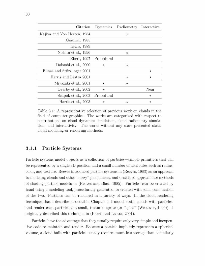
30

Citation Dynamics Radiometry Interactive

Kajiya and Von Herzen, 1984 ?

Gardner, 1985

Lewis, 1989

Nishita et al., 1996 ?

Ebert, 1997 Procedural

Dobashi et al., 2000 ? ?

Elinas and Sturzlinger 2001 ?

Harris and Lastra 2001 ? ?

Miyazaki et al., 2001 ? ?

Overby et al., 2002 ? Near

Schpok et al., 2003 Procedural ?

Harris et al., 2003 ? ? ?

Table 3.1: A representative selection of previous work on clouds in thefield of computer graphics. The works are categorized with respect tocontributions on cloud dynamics simulation, cloud radiometry simula-tion, and interactivity. The works without any stars presented staticcloud modeling or rendering methods.

3.1.1 Particle Systems

Particle systems model objects as a collection of particles—simple primitives that can

be represented by a single 3D position and a small number of attributes such as radius,

color, and texture. Reeves introduced particle systems in (Reeves, 1983) as an approach

to modeling clouds and other “fuzzy” phenomena, and described approximate methods

of shading particle models in (Reeves and Blau, 1985). Particles can be created by

hand using a modeling tool, procedurally generated, or created with some combination

of the two. Particles can be rendered in a variety of ways. In the cloud rendering

technique that I describe in detail in Chapter 6, I model static clouds with particles,

and render each particle as a small, textured sprite (or “splat” (Westover, 1990)). I

originally described this technique in (Harris and Lastra, 2001).

Particles have the advantage that they usually require only very simple and inexpen-

sive code to maintain and render. Because a particle implicitly represents a spherical

volume, a cloud built with particles usually requires much less storage than a similarly

31

detailed cloud represented with other methods. This advantage may diminish as detail

increases, because many tiny particles are needed to achieve high detail. In this situa-

tion other techniques, such as those described in the following sections, may be more

desirable.

3.1.2 Metaballs

Metaballs (or “blobs”) represent volumes as the superposition of potential fields of

a set of sources, each of which is defined by a center, radius, and strength (Blinn,

1982a). These volumes can be rendered in a number of ways, including ray tracing

and splatting. Alternatively, isosurfaces can be extracted and rendered, but this might

not be appropriate for clouds. Nishita et al. used metaballs to model clouds by first

creating a basic cloud shape by hand-placing a few metaballs, and then adding detail via

a fractal method of generating new metaballs on the surfaces of existing ones (Nishita

et al., 1996). Dobashi et al. used metaballs to model clouds extracted from satellite

images (Dobashi et al., 1999). In (Dobashi et al., 2000), clouds simulated on a voxel

grid were converted into metaballs for rendering with splatting.

3.1.3 Voxel Volumes

Voxels are another common representation for clouds. A voxel is the three-dimensional

analog of a pixel. It is a single cell of a regular grid subdivision of a rectangular prism.

Voxel models provide a uniform sampling of the volume, and can be rendered with

both forward and backward methods. There is a large body of existing work on volume

rendering that can be drawn upon when rendering clouds represented as voxel volumes

(Levoy, 1988; Westover, 1990; Wilson et al., 1994; Cabral et al., 1994; Kniss et al.,

2002). Voxel grids are typically used when physically-based simulation is involved.

Kajiya and Von Herzen performed a simple physical cloud simulation and stored the

results in a voxel volume which they rendered using ray tracing (Kajiya and Von Herzen,

1984). Dobashi, et al. simulated clouds on a voxel grid using a cellular automata model

similar to (Nagel and Raschke, 1992), converted the grid to metaballs, and rendered

them using splatting (Dobashi et al., 2000). Miyazaki, et al. 2001 also performed cloud

simulation on a grid using a method known as a Coupled Map Lattice (CML), and

then rendered the resulting clouds in the same way as Dobashi et al. (Miyazaki et al.,

2001). (Overby et al., 2002) solved a set of partial differential equations to generate

clouds on a voxel grid and rendered them using my SkyWorks (Harris and Lastra, 2001)

32

rendering engine. I have solved a similar set of PDEs on a voxel grid using graphics

hardware (Harris et al., 2003). I describe my simulation technique in detail in Chapter

5 and the rendering in Chapter 6.

3.1.4 Procedural Noise

Procedural solid noise techniques are another important technique for generating mod-

els of clouds. These methods use noise as a basis, and perform various operations on

the noise to generate random but continuous density data to fill cloud volumes (Lewis,

1989; Perlin, 1985). Ebert has done much work in modeling “solid spaces” using pro-

cedural solid noise, including offline computation of realistic images of smoke, steam,

and clouds (Ebert and Parent, 1990; Ebert, 1997; Ebert et al., 2002). Ebert modeled

clouds using a union of implicit functions. He then perturbed the solid space defined

by the implicit functions using procedural solid noise, and rendered it using a scan

line renderer. Schpok et al. recently extended Ebert’s techniques to take advantage

of programmable graphics hardware for fast animation and rendering (Schpok et al.,

2003).

3.1.5 Textured Solids

Others have chosen surface representations of clouds rather than volume represen-

tations. Gardner used fractal texturing on the surface of ellipsoids to simulate the

appearance of clouds (Gardner, 1985). By combining multiple textured and shaded

ellipsoids, he was able to create convincing cloudy scenes reminiscent of the landscape

paintings of John Constable. Lewis also used ellipsoids for clouds, but with procedu-

ral solid noise (Lewis, 1989). More recently, Elinas and Sturzlinger used a variation of

Gardner’s method to interactively render clouds composed of multiple ellipsoids (Elinas

and Sturzlinger, 2001).

3.2 Cloud Dynamics Simulation

Cloud simulation has been of interest to meteorologists and atmospheric scientists since

the advent of high performance computing, but it has only recently drawn much interest

from the computer graphics community. Scientific simulations of clouds and weather are

typically very complex, requiring many hours of computation to simulate a relatively

short time of cloud development.

33

The earliest simulations in atmospheric science were simple one-dimensional models

such as the one presented by (Srivastava, 1967). His model represented only vertical

motion and computed changes under the influences of condensation and precipitation.

Later models extended the simulation to two dimensions, but the extreme computa-

tional expense of three dimensions was prohibitive, so researchers tended to resort to

slab symmetry or axial symmetry (Rogers and Yau, 1989). These symmetries limit

simulation to two dimensions, but they at least provide the ability to simulate hor-

izontal wind shear, which is important to cloud dynamics. One of the earliest such

simulations was presented in (Takeda, 1971). Because rotational flow—including vor-

tices with both horizontal and vertical axes of rotation—is common in real clouds, three

dimensional simulation is essential for high accuracy. Steiner presented the first fully

three-dimensional model, and in a comparison with a similar two-dimensional model,

he showed important differences in the rotational motion of the clouds (Steiner, 1973).

Three-dimensional cloud simulation has progressed since then. For a more detailed

survey of cloud simulation in atmospheric physics, see (Rogers and Yau, 1989).

Simulations from atmospheric physics are too expensive for computer graphics ap-

plications other than scientific visualization. Because they are used to understand our

atmosphere and weather, many of them include a high level of detail that is not visible

in nature, including very specific tracking of water state and droplet size distributions,

complex microphysics, and detailed fluid dynamics at a variety of scales. If the goal

is simply to create realistic images and animations of clouds, much less detailed visual

simulations can be used.

Kajiya and Von Herzen were the first in computer graphics to demonstrate a visual

cloud simulation (Kajiya and Von Herzen, 1984). They solved a very simple set of par-

tial differential equations to generate cloud data sets for their ray tracing algorithm.

The PDEs they solved were the Navier-Stokes equations of incompressible fluid flow;

a simple thermodynamic equation to account for advection of temperature and latent

heat effects; and a simple water continuity equation. The simulation required about 10

seconds per time step (one second of cloud evolution) to update a 10× 10× 20 grid on

a VAX 11/780. Overby et al. described a similar but slightly more detailed physical

model based on PDEs (Overby et al., 2002). They used the stable fluid simulation

algorithm of (Stam, 1999) to solve the Navier-Stokes equations. The stability of this

method allows much larger time steps, so Overby et al. were able to achieve simulation

rates of one iteration per second on a 15 × 50 × 15 grid using an 800MHz Pentium

III. I have implemented a faster and slightly more realistic cloud simulation using pro-

34

grammable floating point graphics hardware. This work is described briefly in (Harris

et al., 2003), and in more detail in Chapter 5.

Other researchers have tried simpler, but less realistic rule-based simulation tech-

niques. Neyret used an animated particle system to model cloud behavior, using a set

of heuristics to approximate the rolling behavior of convective clouds (Neyret, 1997).

(Dobashi et al., 2000) used a simple cellular automata (CA) model of cloud forma-

tion to animate clouds offline. The model was based on the simple CA introduced by

(Nagel and Raschke, 1992). Nagel and Raschke’s original CA had rules for the spread

of humidity between neighboring cells and for the formation of clouds in humid cells,

but included no mechanism for evaporation. Dobashi et al. added a stochastic rule

for evaporation so that the clouds would appear to grow and dissipate. Their model

achieved a simulation time of about 0.5 seconds on a 256 × 256 × 20 volume using a

dual 500 MHz Pentium III.

In similar work, Miyazaki et al. used a coupled map lattice (Kaneko, 1993) rather

than a cellular automaton (Miyazaki et al., 2001). This model was an extension of an

earlier coupled map lattice model from the physics literature (Yanagita and Kaneko,

1997). Coupled map lattices (CML) are an extension of CA with continuous state values

at the cells, rather than discrete values. In Chapter 4, I describe work I have done

on performing CML simulations on programmable graphics hardware (Harris et al.,

2002). The CML of Miyazaki et al. used rules based on atmospheric fluid dynamics,

including a rule used to approximate incompressibility and rules for advection, vapor

and temperature diffusion, buoyancy, and phase changes. They were able to simulate

a 3–5 s time step on a 256× 256× 40 lattice in about 10 s on a 1 GHz Pentium III.

Of the previous work in cloud simulation for computer graphics, my work is most

similar to the work by Kajiya and Von Herzen and Overby et al. However, there are

several differences. Both Overby et al. and Kajiya and Von Herzen use a buoyancy

force that is proportional to potential temperature. My model also accounts for the

negative buoyancy effects of condensed water mass and the positive buoyancy effects

of water vapor (see Section 2.1.5). This increases the realism of air currents. Overby

et al. also assume that saturation is directly proportional to pressure, but they pro-

vide no information about how they model pressure in their system. My system uses

a well-known exponential relationship between saturation and temperature (described

in Section 2.1.7), and does not explicitly model pressure. In addition, Overby et al.

introduce two effects that are physically unrealistic. One is a computation meant to ac-

count for the expansion of rising air. The other is an artificial momentum-conservation

35

computation. These computations are superfluous because the Navier-Stokes equations

already account for these phenomena. Overby et al. were able to achieve rates of one

simulation iteration per second. Extrapolating to the fastest current CPU speeds, their

system would likely improve to a few iterations per second. I achieve similar rates

on volumes that are larger by a factor of about 20 (64 × 64 × 64 vs. 15 × 50 × 15)

due to the speed of the graphics hardware. Finally, none of the previous simulations

have been integrated into truly interactive, high frame rate applications. I describe the

integration of cloud simulation with an interactive flight application in Section 5.5.

3.3 Light Scattering and Cloud Radiometry

Some of the earliest work on simulating light scattering for computer graphics was

presented in (Blinn, 1982b). Motivated by the need to render the rings of Saturn,

Blinn described an approximate method for computing the appearance of cloudy or

dusty surfaces via statistical simulation of the light-matter interaction. Blinn made

a simplifying assumption in his model—that the primary effect of light scattering is

due to reflection from a single particle in the medium, and multiple reflections can

be considered negligible. This single scattering assumption has become common in

computer graphics, but as Blinn and others have noted (Bohren, 1987), it is only

valid for media with particles of low single scattering albedo. Blinn also simplified the

problem by limiting application of his model to plane parallel atmospheres, rather than

handling scattering in arbitrary domains.

As I discussed in Chapter 2, accurate computation of light scattering in media

with high single scattering albedo is expensive, because it requires evaluation of a

double integral equation. In practice, researchers either use simplifying assumptions

to reduce the complexity of the problem, or perform long offline computations. There

are multiple ways to compute light scattering, and many simplifications that can be

applied. I will group previous work in this area into five categories: Spherical Harmonics

Methods, Finite Element Methods, Discrete Ordinates, Monte Carlo Integration, and

Line Integral Methods.

3.3.1 Spherical Harmonics Methods

The spherical harmonics Y ml (θ, φ) are the angular portion of the solution of Laplace’s

equation in spherical coordinates (Weisstein, 1999). The spherical harmonics form a

36

complete orthonormal basis. This means that an arbitrary function f(θ, φ) can be

represented by an infinite series expansion in terms of spherical harmonics:

f(θ, φ) =∞∑

l=0

l∑

m=0

Aml Y

ml (θ, φ).

The method of determining the coefficients, Aml , of the series is analogous to deter-

mining the coefficients of a Fourier series expansion of a function. If the value of f

is known at a number of samples, then a series of linear equations can be formulated

and solved for the coefficients. Spherical harmonics methods have been used by (Bhate

and Tokuta, 1992; Kajiya and Von Herzen, 1984; Stam, 1995) to compute multiple

scattering.

Kajiya and Von Herzen presented a ray tracing technique for rendering arbitrary

volumes of scattering media. In addition to a simple single scattering model, they

also described a solution method for multiple scattering that uses spherical harmonics

(Kajiya and Von Herzen, 1984). Their single scattering simulation method stored the

cloud density and illumination data on voxel grids, and their algorithm required two

passes. In the first pass, scattering and absorption were integrated along paths from

the light source through the cloud to each voxel where the resulting intensities were

stored. In the second pass, eye rays were traced through the volume of intensities

and scattering of light to the eye was computed, resulting in a cloud image. For

multiple scattering, the authors derived a discrete spherical harmonics approximation

to the multiple scattering equation, and solved the resulting matrix of partial differential

equations using relaxation. This matrix solution replaces the first integration pass of

the single scattering algorithm. As mentioned in (Stam, 1995), this method is known as

the PN -method in the transport theory literature, where N is the degree of the highest

harmonic in the spherical harmonic expansion.

Following Kajiya and Von Herzen’s lead, two pass algorithms for computing light

scattering in volumetric media—including the algorithms I will present later in this

dissertation—are now common. Interestingly, (Max, 1994) points out that while Kajiya

and Von Herzen attempted to compute multiple scattering for the case of an isotropic

phase function, it is not clear if they succeeded; all of the images in the paper seem to

have been computed with the simpler single scattering model.

Stam explained in (Stam, 1995) that while (Kajiya and Von Herzen, 1984) derived

a very general N -term expression for multiple scattering using a spherical harmonics

37

expansion, they truncated the expansion after the first term to produce their results.

He showed that this truncation results in a diffusion type equation for the scattered

portion of the illumination field. In media where scattering events are very frequent—

“optically thick” media—multiple scattering can be approximated as diffusion of the

light energy. In other words, at any location in the medium, photons can be found

traveling in arbitrary directions. The light is said to be diffuse. Stam presented this

diffusion approximation in more detail. Like Kajiya and Von Herzen, Stam represented

the scattering medium on a voxel grid. He described two ways to solve for the intensity.

In the first method, he discretized the diffusion approximation on the grid to formulate

a system of linear equations that he then solved using the multigrid method. (See

(Briggs et al., 2000) for more information on multigrid methods.) The second method

is a finite element method (see Section 3.3.2) in which he used a series expansion of

basis functions, specifically Gaussian kernel functions of distance. This expansion led

to a matrix system that he solved using LU decomposition.

3.3.2 Finite Element Methods

The finite element method is another technique for solving integral equations that has

been applied to light transport. In the finite element method, an unknown function is

approximated by dividing the domain of the function into a number of small pieces,

or elements, over which the function can be approximated using simple basis functions

(often polynomials). As a result, the unknown function can be represented with a finite

number of unknowns and solved numerically (Cohen and Wallace, 1993).

A common application of finite elements in computer graphics is the radiosity

method for computing diffuse reflection among surfaces. In the radiosity method, the

surfaces of a scene represent the domain of the radiosity function. An integral equation

characterizes the intensity, or radiosity, of light reflected from the surfaces. To solve

the radiosity equation, the surfaces are first subdivided into a number of small elements

on which the radiosity will be represented by a sum of weighted basis functions. This

formulation results in a system of linear equations that can be solved for the weights.

The coefficients of this system are integrals over parts of the surfaces. Intuitively, light

incident on an arbitrary point in the scene can be reflected to any other point; hence

the coefficients are integrals over the scene. In the finite element case, these integrals

are evaluated for every pair of elements in the scene, and are called form factors (Cohen

and Wallace, 1993).

38

Rushmeier and Torrance extended the radiosity method to include radiative transfer

in volumes of participating media (Rushmeier and Torrance, 1987). This zonal method,

like the radiosity method, was originally developed for radiant heat transfer analysis.

The zonal method divides the volume of a participating medium into finite elements

which are assumed to have constant radiosity. As with the radiosity method, form

factors are computed for every pair combination of surface elements in the scene, as

well as every pair of volume elements and all surface-volume pairs. This is complicated

by the fact that the form factors involve a double integral over points in both elements,

as well as along the path between the elements. As in the radiosity method, a system

of simultaneous linear radiosity equations is formulated based on these form factors.

The solution of this system is the steady-state diffuse radiosity at each element of the

environment, including the effects of scattering and absorption by the participating

medium. Rushmeier and Torrance’s presentation of the zonal method was limited to

isotropic scattering media, with no mention of phase functions.

Nishita et al. introduced approximations and a rendering technique for global illu-

mination of clouds, accounting for multiple anisotropic scattering and skylight (Nishita

et al., 1996). This method can also be considered a finite element method, because

the volume is divided into voxels and radiative transfer between voxels is computed.

Nishita et al. made two simplifying observations that reduced the cost of the computa-

tion. The first observation was that the phase function of cloud water droplets is highly

anisotropic, favoring forward scattering (see Section 2.2.5). The result of this is that

not all directions contribute strongly to the illumination of a given volume element.

Therefore, Nishita et al. computed a “reference pattern” of voxels that contributed

significantly to a given point. This pattern is constant at every position in the volume,

because the sun can be considered to be infinitely distant. Thus, the same sampling

pattern can be used to update the illumination of each voxel. The second observation

they made was that only the first few orders of scattering contribute strongly to the

illumination of a given voxel. Therefore, Nishita et al. only computed up to the third

order of scattering. In my cloud illumination algorithms, I also take advantage of the

anisotropy of scattering by cloud droplets (see Chapter 6).

3.3.3 Discrete Ordinates

The method of discrete ordinates allocates the radiosity exiting each volume element

into a collection of M discrete directions. The intensity is assumed to be constant over

39

each direction “bin”. This method can be used to account for anisotropic scattering. If

an interaction between a pair of elements can be represented by only one direction bin

(this is unreasonable for elements that are close), then the number of non-zero elements

in the matrix of linear coefficients is MN2, where N = n3 is the number of elements in

the volume (Max, 1994). Chandresekhar used the discrete ordinates method in early

radiative transfer work (Chandresekhar, 1960). However, Max points out that this

method introduces sampling artifacts because it effectively shoots energy from elements

in infinitesimal beams along the discrete directions, missing the regions between them.

In work inspired by (Patmore, 1993), Max improved on the basic method of discrete

ordinates by efficiently spreading the shot radiosity over an entire direction bin, rather

than along discrete directions. The method achieves a large speedup by handling a

whole plane of source elements simultaneously, which reduces the computation time to

O(MN logN +M2N).

3.3.4 Monte Carlo Integration

Monte Carlo Integration is a statistical method that uses sequences of random numbers

to solve integral equations. In complex problems like light transport, where computing

all possible light-matter interactions would be impossible, Monte Carlo methods reduce

the complexity by randomly sampling the integration domain. With enough samples,

chosen intelligently based on importance, an accurate solution can be found with much

less computation than a complete model would require. The technique of intelligently

choosing samples is called importance sampling, and the specific method depends on

the problem being solved. A common application of Monte Carlo methods in computer

graphics is Monte Carlo ray tracing. In this technique, whenever a light ray traversing a

scene interacts with matter (either a solid surface or a participating medium), statistical

methods are used to determine whether the light is absorbed or scattered (for solids,

this scattering may be thought of as reflection or refraction). If the light is scattered, the

scattered ray direction is also chosen using stochastic methods. Importance sampling

is typically used to determine the direction via the evaluation of a probability function.

A useful introduction to Monte Carlo ray tracing can be found in (Veach, 1997).

Blasi, et al. presented a technique for rendering arbitrary volumes of participating

media using Monte Carlo ray tracing (Blasi et al., 1993). They placed no restrictions

on the medium, allowing arbitrary distributions of density and phase function, and

accounting for multiple scattering. They demonstrated an importance sampling tech-

40

nique that uses the phase function as a probability function to determine the outgoing

direction of scattered rays. This way, the in-scattering integral of Equation (2.27) does

not have to be evaluated over the entire sphere of incoming directions, and a large

amount of computation is saved. Using the phase function for importance sampling

ensures that the most significant contributions of scattering are used to determine the

intensity. In this way, the technique is similar to the “reference pattern” technique used

by (Nishita et al., 1996).

Photon mapping is a variation of pure Monte Carlo ray tracing in which photons

(particles of radiant energy) are traced through a scene (Jensen, 1996). Many photons

are traced through the scene, starting at the light sources. Whenever a photon lands

on a nonspecular surface it is stored in a photon map–a data structure that stores the

position, incoming direction, and radiance of each photon hit. The radiance on a surface

can be estimated at any point from the photons closest to that point. Photon mapping

requires two passes; the first pass builds the photon map, and the second generates an

image from the photon map. Image generation is typically performed using ray tracing

from the eye. The photon map exhibits the flexibility of Monte Carlo ray tracing

methods, but avoids the grainy noise that often plagues them. Jensen and Christensen

extended the basic photon map to incorporate the effects of participating media (Jensen

and Christensen, 1998). To do so, they introduced a volume photon map to store

photons within participating media, and derived a formula for estimating the radiance

in the media using this map. Their techniques enable simulation of multiple scattering,

volume caustics (focusing of light onto participating media caused by specular reflection

or refraction), and color transfer between surfaces and volumes of participating media.

3.3.5 Line Integral Methods

Recently, interest in simulating light scattering has grown among developers of interac-

tive applications. For view-dependent effects and dynamic phenomena, the techniques

described in the previous sections are not practical. While those techniques accurately

portray the effects of multiple scattering, they require a large amount of computation.

For interactive applications, simplifications must be made.

A first step in simplifying the computation is to ignore volumetric scattering alto-

gether. With or without scattering, visualization of the shadowing effects of absorption

by the medium is desirable. This requires at least one pass through the volume (along

the direction of light propagation) to integrate the intensity of transmitted light. Be-

41

cause methods that make this simplification perform the intensity integration along

lines from the light source through the volume, I call them line integral methods. Ka-

jiya and Von Herzen’s original single scattering algorithm, described in Section 3.3.1, is

a line integral method. Intuitively, line integral methods are limited to single scattering

because they cannot propagate light back to points already traversed. In Chapter 6, I

demonstrate that line integral methods can be used to compute multiple scattering in

the forward direction, and that they are therefore useful for interactive cloud rendering.

(Dobashi et al., 2000) described a simple line integral technique for computing the

illumination of clouds using the standard blending operations provided by computer

graphics APIs such as OpenGL (Segal and Akeley, 2001). Dobashi et al. represented

clouds as collections of large “particles” represented by textured billboards. To compute

illumination, they rendered the particles in order of increasing distance from the sun

into an initially white frame buffer. They configured OpenGL blending operations

so that each pixel covered by a particle was darkened by an amount proportional to

attenuation by the particle. After rendering a particle, they read the color of the pixel

at the center of projection of the particle from the frame buffer. They stored this value

as the intensity of incident light that reached the particle through the cloud. Traversal

of the particles in order of increasing distance from the light source evaluates the line

integral of extinction through each pixel (see Chapter 6). Because pixels are darkened

by every particle that overlaps them, this method computes accurate self-shadowing of

the cloud. After this first pass, they rendered particles from back to front with respect

to the view point, using the intensities computed in the first pass. They configured

blending to integrate absorption and single scattering along lines through each pixel of

the image, resulting in a realistic image of the clouds. Dobashi et al. further enhanced

this realism by computing the shadowing of the terrain by the clouds and shafts of light

between the clouds.

As I mentioned previously, the volume must be traversed at least once to integrate

attenuation due to absorption. During this traversal, it makes sense to also integrate

scattering along the direction of traversal. In Chapter 6, I show how the method of

(Dobashi et al., 2000) can be extended to compute this multiple forward scattering.

I originally presented this technique in (Harris and Lastra, 2001), and extended it to

voxel clouds in (Harris et al., 2003).

Kniss, et al. presented a similar line integral approach for absorption and multiple

forward scattering in the context of direct volume rendering (Kniss et al., 2002). They

rendered volumes of translucent media from 3D textures by rendering slices of the

42

volume oriented to face along the halfway vector between the light and view directions.

This “half angle slice” technique allowed them to interleave light transport integration

with the display of the volume. The method traverses the volume slices in order of

increasing distance from the light source, performing alternate display and illumination

passes. Three buffers are maintained: two for the computation of the illumination of

the volume (current and next), and one (typically the frame buffer) for display of the

volume. During the display pass, the current slice is rendered from the observer’s point

of view. The slice is textured with the 3D volume texture blended with the current

illumination buffer. This results in self-shadowing of the volume as in (Dobashi et al.,

2000), as well as incorporating the scattering computed during the illumination pass

as in (Harris and Lastra, 2001). During the illumination pass, the slice is rendered

into the next illumination buffer from the light’s point of view, and blended with the

current illumination buffer to compute the next step in the line integral of extinction

and forward in-scattering. During this blending, the current buffer is sampled multiple

times at jittered locations, and the samples are averaged. This accomplishes a blurring

of the forward-scattered light—an ad hoc approximation of multiple scattering over a

small solid angle around the forward direction. Even though this method is ad hoc, it

is physically-based because multiple scattering in media with a high single scattering

albedo results in “blurring” of the light intensity (the light is diffuse).

Chapter 4

Physically-Based Simulation on

Graphics Hardware

Interactive 3D graphics environments, such as games, virtual environments, and flight

simulators are becoming increasingly visually realistic, in part due to the power of

graphics hardware. However, these applications often lack rich dynamic phenomena,

such as fluids, clouds, and smoke, which are common in the real world. A large body

of work in computer graphics has been dedicated to simulating and modeling natural

dynamics. One of my goals has been to accelerate such physically-based simulations

by performing the computation on graphics hardware.

Graphics hardware is an efficient processor of images—it can use texture images as

input, and it outputs images via rendering. Techniques for physically-based simulation

of volumetric dynamic phenomena often represent the state of simulations as grids

or lattices of values. Images—arrays of values—map well to state values on a grid.

Two-dimensional lattices can be represented by 2D textures, and 3D lattices can be

represented by 3D textures or collections of 2D textures. This natural correspondence,

as well as the programmability and performance of graphics hardware, motivated my

research.

In this chapter I discuss techniques for simulation of dynamic phenomena on graph-

ics hardware. Section 4.1 motivates the use of graphics hardware for general purpose

computation, and Section 4.1.2 describes previous work in this area. Air is a fluid,

so cloud dynamics are first and foremost fluid dynamics. In Section 4.2 I discuss the

solution of the Navier-Stokes equations for incompressible fluid flow. I then describe in

detail some techniques for performing fluid simulation on a Graphics Processing Unit

(GPU). In the next chapter, I discuss the application of these techniques to cloud sim-

44

ulation. In Section 4.3 I discuss methods for performing physically-based simulation

on the previous, less-capable generation of GPUs.

4.1 Why Use Graphics Hardware?

GPUs are designed to be efficient coprocessors for rendering and shading. The pro-

grammability now available in GPUs such as the NVIDIA GeForce FX (NVIDIA Cor-

poration, 2003) and the ATI Radeon 9800 (ATI Technologies, Inc., 2003) makes them

useful coprocessors for more diverse applications. Because the time between new gener-

ations of GPUs is currently much less than for CPUs, faster coprocessors are available

more often than faster central processors (see Figure 4.1). GPU performance tracks

rapid improvements in semiconductor technology more closely than CPU performance.

This is because CPUs are designed for low latency computations, while GPUs are op-

timized for high throughput of vertices and fragments (Lindholm et al., 2001). Low

latency on memory-intensive applications typically requires large caches, which use a lot

of silicon area. Additional transistors are used to greater effect in GPU architectures

because they are applied to additional processors and functional units that increase

throughput. In addition, programmable GPUs are inexpensive, readily available, easily

upgradeable, and compatible with multiple operating systems and hardware architec-

tures.

More importantly, interactive computer graphics applications have many compo-

nents vying for processing time. Often it is difficult to efficiently perform simulation,

rendering, and other computational tasks simultaneously without a drop in perfor-

mance. Because my intent is visual simulation, rendering is an essential part of any

solution. Moving simulation onto the GPU that renders the results of a simulation not

only reduces computational load on the main CPU, but also avoids the substantial bus

traffic required to transmit the results of a CPU simulation to the GPU for rendering.

In this way, methods of dynamic simulation on the GPU provide an additional tool for

load balancing in complex interactive applications.

Graphics hardware also has disadvantages. My first work on GPU simulation was

done in collaboration with Greg Coombe, Thorsten Scheuermann, and Anselmo Lastra

(Harris et al., 2002). In this work, we used NVIDIA GeForce 3 (NVIDIA Corporation,

2001) and GeForce 4 (NVIDIA Corporation, 2002a) GPUs. The main problems we

encountered with these GPUs were the difficulty of programming them and the lack

of high precision fragment operations and storage. These problems were related—

45

Figure 4.1: A graph of performance increase over time for CPUs and GPUs. GPUperformance has increased at a faster rate than CPUs. (Graph and data courtesy ofAnselmo Lastra.)

programming difficulty increased with the effort required to ensure that we conserved

precision wherever possible.

Within a year of our first experiments, these issues were mostly resolved by the latest

GPUs and software. Following a recent research trend in the use of high-level shading

languages to program graphics hardware (Peercy et al., 2000; Proudfoot et al., 2001),

NVIDIA released its Cg shading language (Mark et al., ). Cg has greatly increased

the ease with which GPUs can be used for general-purpose computation. Also, the

new generation of GPUs, the NVIDIA GeForce FX series (NVIDIA Corporation, 2003)

and the ATI Radeon 9700/9800 (ATI Technologies, Inc., 2003), provide floating point

precision throughout the graphics pipeline. This has enabled the application of GPUs

to high-fidelity visual simulations of natural phenomena and other systems of partial

differential equations that require storage and computation of high dynamic range

numbers. Previously, the lack of floating point capability limited the application of

GPUs to either low dynamic range simulations or more ad hoc techniques such as

cellular automata (Harris et al., 2002). Future generations of GPUs will likely continue

46

to improve in flexibility and performance.

4.1.1 Classes of GPUs

Graphics processors are evolving rapidly. Manufacturers such as NVIDIA and ATI

typically launch a new architecture once a year, with an update about six months later.

As a result I have used processors of varying speed and capability in my research. In

this chapter, I discuss techniques for performing physically-based simulation on two

generations of GPUs. To improve clarity, I will rely on a common classification used in

the graphics industry.

There are two standard graphics programming interfaces that are used for most

commercial applications: OpenGL (Segal and Akeley, 2001) and DirectX (DX) (Mi-

crosoft, 2003). While the core of OpenGL does not change very often,1 Microsoft has

released new versions of DirectX on a schedule very similar to GPU release schedules.

As a result, it has become convenient to classify GPUs by the DirectX version that

they support. In what follows, I will use the following classification of GPUs.

Pre-DX8 GPUs These GPUs are not programmable beyond advanced texture

blending capabilities, and fragment precision is limited to eight bits per channel. This

class includes NVIDIA GPUs prior to the GeForce 3, and ATI GPUs prior to the

Radeon 8500. Per-pixel lighting and bump mapping require multiple passes on these

processors.

DX8 GPUs These GPUs are the first to include an assembly language for vertex

processing (“vertex programs” or “vertex shaders”). Vertex programs cannot branch.

Fragment precision is limited to eight bits per channel, except for some proprietary 16-

bit dual channel formats. Fragment and texture processing is much more configurable,

with enough functionality for simple programmability. Bump mapping and simple per-

pixel lighting models can be computed in a single pass. Examples of DX8 GPUs are

the ATI Radeon 8500 and NVIDIA GeForce 3.

DX9 GPUs These GPUs extend vertex programs to enable data-dependent branch-

ing, and add a fragment program assembly language. Fragment programs cannot

branch, but support conditional writes of the result of instructions. Floating point

1Nevertheless, new GPU features are typically exposed earlier in OpenGL, through its standardizedextension protocol.

47

fragment precision is now supported, although not standardized.2 Complex rendering,

shading, and even simulation operations can be computed in a single pass. Examples

of DX9 GPUs are the NVIDIA GeForce FX 5900 Ultra and the ATI Radeon 9800.

DX9+ GPUs The first of these GPUs are in production as I write this, but their

details have not been announced. One can speculate on the features these processors

will introduce, such as branching in fragment programs, or the ability to read texture

memory in vertex programs. More advanced features may include primitive- or object-

level programmability, with the ability to generate vertices on the fly. Whether GPUs

will move further toward general-purpose programmability or continue to add more

advanced application specific functionality—for example, custom support for global

illumination algorithms—remains to be seen.

4.1.2 General-Purpose Computation on GPUs

The use of computer graphics hardware for general-purpose computation has been an

area of active research for many years, beginning on machines like the Ikonas (England,

1978), the Pixel Machine (Potmesil and Hoffert, 1989), and Pixel-Planes 5 (Rhoades

et al., 1992). The wide deployment of GPUs in the last several years has resulted in an

increase in experimental research with graphics hardware. Trendall and Steward give

a detailed summary of the types of computation available on modern GPUs (Trendall

and Steward, 2000).

Within the realm of graphics applications, programmable graphics hardware has

been used for procedural texturing and shading (Rhoades et al., 1992; Olano and Lastra,

1998; Peercy et al., 2000; Proudfoot et al., 2001). Graphics hardware has also been

used for volume visualization (Cabral et al., 1994; Wilson et al., 1994; Kniss et al.,

2002). Recently, new methods have been developed for using current GPUs for global

illumination, including ray tracing (Carr et al., 2002; Purcell et al., 2002), photon

mapping (Purcell et al., 2003), and radiosity (Carr et al., 2003; Coombe et al., 2003).

Other researchers have found ways to use graphics hardware for non-graphics ap-

plications. The use of rasterization hardware for robot motion planning was described

in (Lengyel et al., 1990). (Hoff et al., 1999) described the use of z-buffer techniques for

the computation of Voronoi diagrams. The PixelFlow SIMD graphics computer (Eyles

et al., 1997) was used to crack UNIX password encryption (Kedem and Ishihara, 1999),

2The ATI Radeon 9700/9800 provides 24-bit (per channel) floating point, while the NVIDIAGeForce FX family supports 16- and 32-bit formats.

48

and graphics hardware has been used in the computation of artificial neural networks

(Bohn, 1998).

My initial work in this area used a Coupled Map Lattice (CML) to simulate dynamic

phenomena that can be described by partial differential equations. Related to this is the

visualization of flows described by PDEs, which has been implemented using graphics

hardware to accelerate line integral convolution and Lagrangian-Eulerian advection

(Heidrich et al., 1999; Jobard et al., 2001; Weiskopf et al., 2001). Greg James of

NVIDIA has demonstrated the “Game of Life” cellular automata and a 2D physically-

based water simulation running on NVIDIA GPUs (James, 2001a; James, 2001b; James,

2001c). More recently, Kim and Lin used GPUs to simulate dendritic ice crystal growth

(Kim and Lin, 2003), and Li et al. used them to perform Lattice Boltzmann simulation

of fluid flow (Li et al., 2003).

Research on general-purpose uses of GPUs, which I call “GPGPU”, has seen a mi-

nor boom in the time since we began our work on simulation using GPUs. Strzodka

showed how to combine multiple 8-bit texture channels to create virtual 16-bit precise

operations (Strzodka, 2002). Level set segmentation of images and volume data on

GPUs has been demonstrated by (Strzodka and Rumpf, 2001; Lefohn and Whitaker,

2002; Lefohn et al., 2003). Other recent GPGPU research includes image-based mod-

eling (Yang et al., 2002; Hillesland et al., 2003), collision detection (Hoff et al., 2001;

Govindaraju et al., 2003), and computational geometry (Mustafa et al., 2001; Krishnan

et al., 2002; Guha et al., 2003; Stewart et al., 2003).

Researchers have recently embraced the power of the GPU for performing ma-

trix computations. Larsen and McAllister used texturing operations to perform large

matrix-matrix multiplies (Larsen and McAllister, 2001). This work preceded our own,

and was mostly a proof-of-concept application, because they used GPUs without sup-

port for floating point textures. Thompson, et al. used the programmable vertex

processor of an NVIDIA GeForce 3 GPU to solve the 3-Satisfiability problem and to

perform matrix multiplication (Thompson et al., 2002). Others have used the GPU to

solve sparse linear systems, using techniques such as Red-Black Jacobi iteration, Conju-

gate Gradient and multigrid methods (Bolz et al., 2003; Goodnight et al., 2003; Harris

et al., 2003; Kruger and Westermann, 2003). These four papers also all demonstrate

fluid simulation on the GPU.

This wide variety of applications demonstrates that the GPU has become an ex-

tremely powerful computational workhorse. It is especially adept at SIMD computation

applied to grid or matrix data. The GPU has proven to be a nearly ideal platform for

49

Figure 4.2: Colored “dye” carried by a swirling fluid. The inset images show the velocityfield of each fluid. Velocity in the x and y directions are stored in the red and greencolor channels, respectively.

visual simulation of fluids, which I discuss in the following section. I extend the simu-

lation to clouds in Chapter 5.

4.2 Fluid Simulation on the GPU

Clouds are only one example of fluids in nature; other examples include the flow of

rivers, smoke curling from a glowing cigarette, steam rushing from a teapot, weather

patterns, and the mixing of paint. All are phenomena that we would like to portray

realistically in interactive graphics applications. Fluid simulation is a useful building

block that is the starting point to simulating a variety of natural phenomena. Because

of the large amount of parallelism in graphics hardware and the parallel nature of the

computations required to simulate fluids, fluid simulation can be performed significantly

faster on GPUs than on CPUs. Using an NVIDIA GeForce FX, I have achieved a two- to

four-times speedup over an equivalent CPU simulation. Figure 4.2 shows some results

from my simple GPU fluid simulator.

The techniques I describe are based on the“Stable Fluids” method of (Stam, 1999).

However, while Stam’s simulations used a CPU implementation, I use graphics hard-

ware because GPUs are well suited to the type of computations required by fluid simu-

50

lation. The simulation I describe is performed on a grid of cells. Programmable GPUs

are designed to perform computations on pixels, which can be used to represent a grid

of cells. GPUs achieve high performance because they contain multiple simple proces-

sors that can process several pixels in parallel. They are also optimized to perform

multiple texture lookups per cycle. Because my simulation grids are stored in textures,

this speed and parallelism are just what I need for fast fluid simulation.

The scope of the simulation concepts that I can cover here is necessarily lim-

ited. Cloud simulation requires simulation of a continuous volume of fluid on a two-

dimensional rectangular domain, and I use these requirements to limit my discussion.

I do not simulate free surface boundaries between fluids, such as the interface between

sloshing water and air, because clouds are a mixture of air, water vapor, and condensed

water droplets. There are many extensions to the basic techniques I use, some of which

I mention later in this chapter.

4.2.1 The Navier-Stokes Equations

The most important quantity to represent in a fluid simulation is the velocity of the

fluid, because velocity determines how the fluid moves itself and the things that are in it.

I define the velocity vector field of a fluid on a Cartesian grid such that for every discrete

position ~x = (x, y), there is an associated velocity at time t, ~u(~x, t) = (u(~x, t), v(~x, t)),

as shown in Figure 4.3. I restrict discussion here to two dimensions for simplicity.

Extension of the mathematics to three dimensions is straightforward. In the next

chapter, I discuss issues in implementing 3D fluid simulations on the GPU.

The key to fluid simulation is to take steps in time, and at each time step, correctly

determine the current velocity field. I do this by solving the Navier-Stokes equations

for incompressible flow. Once I have the velocity field, I can do interesting things with

it, like use it to move objects, smoke densities, cloud water concentrations, and other

quantities that can be displayed in applications. For the sake of convenience, I repeat

the Navier-Stokes equations here. Refer to Section 2.1.1 for more details.

∂~u

∂t= − (~u ·∇) ~u−

1

ρ∇p+ ν∇2~u+ ~F (4.1)

∇· ~u = 0 (4.2)

As described in Chapter 2, the four terms on the right-hand side of Equation 4.1 repre-

sent acceleration due to advection, pressure, diffusion, and external forces, respectively.

51

(0,N-1) (1,N-1) (2,N-1) (M-1,N-1)

(0,2) (1,2) (2,2) (M-1,2)

(0,1) (1,1) (2,1) (M-1,1)

(0,0) (1,0) (2,0) (M-1,0)

δx

δy

Figure 4.3: The state of the fluid simulation is represented on an M ×N grid like theone shown here. The arrows represent velocity.

I will return to the Navier-Stokes equations after a quick review of the vector calculus

needed to solve them. For a detailed derivation and more details, I recommend (Chorin

and Marsden, 1993) and (Griebel et al., 1998).

Visual simulation of fluids has recently been a popular topic of computer graphics

research. Foster and Metaxas presented techniques for simulating the motion of hot

gases (Foster and Metaxas, 1997). Stam described a stable numerical technique for

interactive simulation of fluid motion (Stam, 1999). The method I use for fluid simula-

tion on the GPU is based on Stam’s algorithm. Fedkiw, et al. extended Stam’s stable

fluid simulation techniques to simulate realistic smoke (Fedkiw et al., 2001). My cloud

simulation implements some key features of their simulation on the GPU.

4.2.2 A Brief Vector Calculus Review

Equations 4.1 and 4.2 contain three different uses of the symbol ∇ (often pronounced

“del”), which is also known as the nabla operator. The three applications of nabla are

the gradient, divergence, and Laplacian operators, as shown in Table 1. The subscripts

52

Operator Type Definition Finite Difference Form

Gradient Scalar ∇p =(

∂p∂x, ∂p

∂y

)

∇p =(

pi+1,j−pi−1,j

2δx,

pi,j+1−pi,j−1

2δy

)

Divergence Vector ∇·u = ∂u∂x

+ ∂v∂y

∇·u =ui+1,j−ui−1,j

2δx+

vi,j+1−vi,j−1

2δy

Laplacian Scalar ∇2p = ∂2p∂x2 + ∂2p

∂y2 ∇2p =pi+1,j−2pi,j+pi−1,j

(δx)2+

pi,j+1−2pi,j+pi,j−1

(δy)2

Table 4.1: Vector calculus operators used in fluid simulation.

i and j used in the expressions in the table refer to discrete locations on a Cartesian

grid, and δx and δy are the grid spacing in the x and y dimensions, respectively (see

Figure 4.3).

The gradient of a scalar field is a vector of partial derivatives of the scalar field.

Divergence, which appears in Equation (4.2), has an important physical significance.

It is the rate at which “density” exits a given region of space. In the Navier-Stokes

equations it is applied to the velocity of the flow, and measures the net change in

velocity across a surface surrounding a small piece of the fluid. Equation (4.2), the

continuity equation, enforces the incompressibility assumption by ensuring that the fluid

always has zero divergence. This means that velocity is neither created nor destroyed

(except by external forces), and that momentum is conserved. The dot product in the

divergence operator results in a sum of partial derivatives (rather than a vector, as with

the gradient operator). This means that the divergence operator can only be applied

to a vector field, such as the velocity ~u = (u, v).

Notice that the gradient of a scalar field is a vector field, and the divergence of a

vector field is a scalar field. If the divergence operator is applied to the result of the

gradient operator, the result is the Laplacian operator ∇·∇ = ∇2. If the grid cells are

square (δx = δy, which we assume for the remainder of this dissertation), the Laplacian

simplifies to

∇2p =pi+1,j + pi−1,j + pi,j+1 + pi,j−1 − 4pi,j

(δx)2 (4.3)

The Laplacian operator appears commonly in physics, most notably in the form

of diffusion equations, such as the heat equation. Equations of the form ∇2x = b are

known as Poisson equations. The case where b = 0 is Laplace’s Equation, which is

the origin of the Laplacian operator. In Equation (4.1), the Laplacian is applied to a

53

vector field. This is a notational simplification—the operator is applied separately to

each scalar component of the vector field.

4.2.3 Solving the Navier-Stokes Equations

Analytical solutions of the Navier-Stokes equations can only be found for a few simple

physical configurations. However, it is possible to use numerical integration techniques

to solve them incrementally. My goal is to display the evolution of the flow over time, so

an incremental numerical solution works well. The algorithm I use to solve the Navier-

Stokes equations is based on the “stable fluids” technique described in (Stam, 1999).

In this section I describe the mathematics of each step in the algorithm, following the

derivations presented in (Chorin and Marsden, 1993; Stam, 1999). In Section 4.2.4 I

describe my implementation on the GPU using the Cg shading language (Mark et al.,

).

First I need to transform the equations into a form that is more amenable to nu-

merical solution. Recall that the two-dimensional Navier-Stokes equations are three

equations that we can solve for the quantities u, v, and p. However it is not obvious

how to solve them. The following section describes a transformation that leads to a

straightforward algorithm.

The Helmholtz-Hodge Decomposition

Basic vector calculus says that any vector ~v can be decomposed into a set of basis

vector components whose sum is ~v. For example, we commonly represent vectors on a

Cartesian grid as a pair of distances along the grid axes: ~v = (x, y). The same vector

can be written ~v = xı + y, where ı and are unit basis vectors aligned to the axes of

the grid.

In the same way that we can decompose a vector into a sum of vectors, we can also

decompose a vector field into a sum of vector fields. Let D be the region in space, or

in this case the plane, on which a fluid is defined. Let this region have a smooth (in

other words, it has no discontinuities) boundary, ∂D, with normal direction n. We can

use the following theorem.

Helmholtz-Hodge Decomposition Theorem A vector field ~w on D can be uniquely

decomposed in the form

~w = ~u+∇p (4.4)

54

where ~u has zero divergence and is parallel to ∂D; that is, ~u · n = 0 on ∂D.

I use the theorem without proof. For details and a proof of this theorem, refer to

Section 1.3 of (Chorin and Marsden, 1993).

This theorem states that any vector field can be decomposed into the sum of two

other vector fields: a divergence-free vector field, and the gradient of a scalar field. It

is a powerful tool, leading to two useful realizations.

First Realization Solution of the Navier-Stokes equations involves several computa-

tions to update the velocity at each time step: advection, diffusion and force application.

The result is a new velocity field, ~w, with nonzero divergence. But the continuity equa-

tion requires that each time step ends with a divergence-free velocity. Fortunately, the

Helmholtz-Hodge Decomposition Theorem states that the divergence of the velocity

can be corrected by subtracting the gradient of the pressure field:

~u = ~w −∇p. (4.5)

Second Realization The theorem also leads to a method for computing the pressure

field. If we apply the divergence operator to both sides of Equation (4.4), we obtain

∇· ~w = ∇· (~u+∇p) = ∇· ~u+∇2p.

But Equation (4.2) enforces that ∇· ~u = 0, so this simplifies to

∇2p = ∇· ~w, (4.6)

which is a Poisson equation (see Section 4.2.2) for the pressure of the fluid, sometimes

called the Poisson-pressure equation. This means that after we arrive at our divergent

velocity, ~w, we can solve Equation (4.6) for p, and then use ~w and p to compute the

new divergence free field, ~u, using Equation (4.5). We return to this later.

Now we need a way to compute ~w. To do this, we return to the comparison of vectors

and vector fields. We know, given the definition of the dot product, that we can find

the projection of a vector ~r onto a unit vector s by computing the dot product of ~r

and s. The dot product is a projection operator for vectors that maps a vector ~r onto

its component in the direction of s. We can use the Helmholtz-Hodge Decomposition

Theorem to define a projection operator, P, that projects a vector field ~w onto its

55

divergence-free component, ~u. If we apply P to Equation (4.4), we get

P~w = P~u+ P (∇p) .

However, by the definition of P, P~w = P~u = ~u. Therefore, P (∇p) = 0. Now we use

these ideas to simplify the Navier-Stokes equations.

First, apply the new projection operator to both sides of Equation (4.1):

P∂~u

∂t= P

(

−(~u ·∇)~u−1

ρ∇p+ ν∇2~u+ ~F

)

.

Because ~u is divergence-free, so is the derivative on the left-hand side, so P (∂~u/∂t) =

∂~u/∂t. Also, P (∇p) = 0, so the pressure term drops out. We are left with the following

equation:∂~u

∂t= P

(

−(~u ·∇)~u+ ν∇2~u+ ~F)

. (4.7)

The great thing about this equation is that it symbolically encapsulates the algo-

rithm for simulating fluid flow. We first compute what is inside the parentheses on

the right-hand side. From left to right, we compute the advection, diffusion, and force

terms. Application of these three steps results in a divergent velocity field, ~w, to which

we apply the projection operator P to get a new divergence-free field, ~u. To do so, we

solve Equation (4.6) for p, and then subtract the gradient of p from ~w as in Equation

(4.5).

In a typical implementation, the various components are not computed and added

together, as in Equation (4.7). Instead, the solution is found via composition of trans-

formations on the state; in other words, each component is a step that takes a field as

input, and produces a new field as output. We can define an operator S which is equiv-

alent to the solution of Equation (4.7) over a single time step. The operator is defined

as the composition of operators for advection (A), diffusion (D), force application (F),

and projection (P):

S = P ◦ F ◦ D ◦ A (4.8)

Thus, a step of the simulation algorithm can be expressed as S(~u) = P ◦ F ◦ D ◦

A(~u). The operators are applied right-to-left; first advection, followed by diffusion,

force application and projection. This is exactly the algorithm that I describe in Section

4.2.4. Note that time is omitted above for clarity, but in practice, the time step must

56

be used in the computation of each operator. Next I look more closely at the advection

and diffusion steps, and then approach the solution of the Poisson equations.

Advection

Advection is the process by which a fluid’s velocity transports itself and other quantities

in the fluid. To compute the advection of a quantity, we must update the quantity at

each grid point. Because we are computing how a quantity moves along the velocity

field, it helps to imagine that each grid cell is represented by a particle. A first attempt

at computing the result of advection might be to update the grid as we would update a

particle system. Just move the position, ~r, of each particle forward along the velocity

field the distance it would travel in time δt:

~r(t+ δt) = ~r(t) + ~u(t)δt.

This is Euler’s method ; it is a simple method for explicit (or forward) integration

of ordinary differential equations. (There are more accurate methods, such as the

midpoint method and the Runge-Kutta methods.)

There are two problems with this approach: The first is that simulations that use

explicit methods for advection are unstable for large time steps, and can “blow up”

if the magnitude of ~u(t)δt is greater than the size of a single grid cell. The second

problem is specific to GPU implementation. I implement my simulation in fragment

programs, which cannot change the image-space output location of the fragments they

write. This forward-integration method requires the ability to “move” the particle at

each grid cell, so it cannot be implemented on current GPUs.

The solution is to invert the problem and use an implicit method (Stam, 1999).

Rather than advecting quantities by computing where a particle moves over the current

time step, trace the trajectory of the particle from each grid cell back in time to its

former position, and copy the quantities at that position to the starting grid cell. To

update a quantity q (this could be velocity, density, temperature, or any quantity

carried by the fluid), use the following equation:

q (~x, t+ δt) = q (~x− ~u (~x, t) δt, t) . (4.9)

Not only is this method easily implemented on the GPU, but as Stam showed,

it is stable for arbitrary time steps and velocities. Figure 4.4 depicts the advection

57

u(x,t) u(x,t)δt

Figure 4.4: Computing fluid advection.

computation at the cell marked with a circle. Tracing the velocity field back in time

leads to an ‘x.’ The four grid values nearest the ‘x’ (connected by a dashed square in

the figure) are bilinearly interpolated and the result is written to the starting grid cell.

Viscous Diffusion

As explained in Chapter 2, viscous fluids have a certain amount of resistance to flow,

which results in diffusion (or dissipation) of velocity. A partial differential equation for

viscous diffusion is∂~u

∂t= ν∇2~u. (4.10)

As in advection, there are multiple ways to solve this equation. An obvious approach

is to formulate an explicit, discrete form in order to develop a simple algorithm:

~u(~x, t+ δt) = ~u(~x, t) + νδt∇2~u(~x, t).

In this equation ∇2 is the discrete form of the Laplacian operator, Equation (4.3). Like

the explicit Euler method for computing advection, this method is unstable for large

values of δt and ν (Stam, 2003). I use Stam’s implicit formulation of Equation (4.10):

(

I− νδt∇2)

~u (~x, t+ δt) = ~u (~x, t) . (4.11)

58

Here, I is the identity matrix. This formulation is stable for arbitrary time steps and

viscosities. Equation (4.11) is a (somewhat disguised) Poisson equation for velocity.

Remember that the use of the Helmholtz-Hodge decomposition results in a Poisson

equation for pressure. These equations can be solved using an iterative relaxation

technique.

Solution of Poisson Equations

There are two Poisson equations that I must solve: the Poisson-pressure equation and

the viscous diffusion equation. Poisson equations are common in physics and are well

understood. I use an iterative solution technique that starts with an approximate

solution and improves it every iteration.

The Poisson equation is a matrix equation of the form A~x = ~b, where ~x is the vector

of unknown values (p or ~u in this case); ~b is a vector of constants; and A is a matrix.

In the Poisson equations, A is implicitly represented in the Laplacian operator ∇2 , so

it need not be explicitly stored as a matrix. Iterative solution techniques start with an

initial “guess” for the solution, ~x(0), and each step k produces an improved solution,

~x(k). The superscript notation indicates the iteration number. The simplest iterative

technique is called Jacobi iteration. A derivation of Jacobi iteration for general matrix

equations can be found in (Golub and Van Loan, 1996).

More sophisticated methods (such as Conjugate Gradient and multigrid) converge

faster, but I use Jacobi iteration because of its simplicity and ease of implementation.

For details and examples of more sophisticated solvers, see (Bolz et al., 2003; Goodnight

et al., 2003; Kruger and Westermann, 2003).

Equations (4.6) and (4.11) appear different, but both can be discretized using Equa-

tion (4.3) and rewritten in the form

x(k+1)i,j =

x(k)i−1,j + x

(k)i+1,j + x

(k)i,j−1 + x

(k)i,j+1 + αbi,j

β, (4.12)

where α and β are constants. The values of x, b, α, and β are different for the two

equations. In the Poisson-pressure equation, x represents pδt,3 b represents ∇· ~w,

α = (δx)2, and β = 4. For the viscous diffusion equation, x and b both represent ~u,

α = (δx)2/νδt, and β = 4 + α.

3Note that the solution of this equation is actually pδt, not p. This is not a problem, becausethis pressure serves only to compute the pressure gradient used in the projection step. Because δt isconstant over the grid, it does not affect the gradient.

59

I formulate the equations this way because it lets me use the same code to solve

both equations. To solve the equations, I simply run a number of iterations in which

I apply Equation (4.12) at every grid cell, using the results of the previous iteration

as input to the next (x(k+1) becomes x(k)). Because Jacobi iteration converges slowly,

I need to execute many iterations. Fortunately, Jacobi iterations are cheap to execute

on the GPU, so I can run many iterations in a very short time.

Initial and Boundary Conditions

Any differential equation problem defined on a finite domain requires boundary condi-

tions in order to be well-posed. The boundary conditions determine how values at the

edges of the simulation domain are computed. Also, to compute the evolution of the

flow over time, we must know how it started—in other words, its initial conditions. For

my fluid simulation, I assume the fluid initially has zero velocity and zero pressure (that

is, zero deviation from the environmental pressure) everywhere. Boundary conditions

require a bit more discussion.

During each time step, I solve equations for two quantities—velocity and pressure—

and I need boundary conditions for both. Because my fluid is simulated on a rectangular

grid, I assume that it is a fluid in a box and cannot flow through the sides of the box.

For velocity, I use the no-slip condition, which specifies that velocity goes to zero at

the boundaries4. The correct solution of the Poisson-pressure equation requires pure

Neumann boundary conditions: ∂p/∂n = 0. This means that at a boundary, the rate of

change of pressure in the direction normal to the boundary is zero. I revisit boundary

conditions at the end of Section 4.2.4.

4.2.4 Implementation

Now that I have described the problem and the basics of solving it, I can move forward

with the implementation. A good place to start is to lay out some pseudocode for the

algorithm. The algorithm is the same every time step, so this pseudocode represents a

single time step. The variables u and p hold the velocity and pressure field data.

// Apply the first 3 operators in Equation (4.8).

u = advect(u);

u = diffuse(u);

4In cloud simulation, as I describe in Chapter 5, I use no-slip conditions only along the ground.

60

u = addForces(u);

// Now apply the projection operator to the result.

p = computePressure(u);

u = subtractPressureGradient(u, p);

In practice, temporary storage is needed because most of these operations cannot

be performed in place. For example, the advection step in the pseudocode is more

accurately written as

uTemp = advect(u);

swap(u, uTemp);

This pseudocode contains no implementation-specific details. In fact, the same pseu-

docode describes CPU and GPU implementations equally well. My goal is to perform

all steps on the GPU. In order to clarify this type of general-purpose computation on

GPUs, in the next section I make some analogies between operations in a typical CPU

fluid simulation and their counterparts on the GPU.

CPU-GPU Analogies

Fundamental to any computer are its memory and processing models, so any applica-

tion must consider data representation and computation. In this section I discuss the

differences between CPUs and GPUs with regard to both of these.

Textures = Arrays My simulation represents data on a two-dimensional grid. The

natural representation for this grid on the CPU is an array. The analog of an array on

the GPU is a texture. Although textures are not as flexible as arrays, their flexibility is

improving as graphics hardware evolves. Textures on current GPUs support all basic

operations necessary to implement a fluid simulation. Because textures usually have

three or four color channels, they provide a natural data structure for vector data types

with two to four components. Alternatively, multiple scalar fields can be stored in

a single texture. The most basic operation is an array (or memory) read, which is

accomplished by using a texture lookup. Thus, the GPU analog of an array index is a

texture coordinate.

Loop Bodies = Fragment Programs A CPU implementation of the simulation

performs the steps in the algorithm by looping, using a pair of nested loops to iterate

61

over each cell in the grid as in (Stam, 2003). At each cell, the same computation

is performed. GPUs do not have the capability to perform this inner loop over each

texel in a texture. However, the fragment pipeline is designed to perform identical

computations at each fragment. To the programmer, it appears as if there is a processor

for each fragment, and that all fragments are updated simultaneously. In the parlance of

parallel programming, this model is known as Single Instruction Multiple Data (SIMD)

computation. Thus, the GPU analog of computation inside nested loops over an array

is a fragment program applied in SIMD fashion to each fragment.

Feedback = Texture Update In Section 4.2.3, I described how I use Jacobi iter-

ation to solve Poisson equations. This type of iterative method uses the result of an

iteration as input for the next iteration. This feedback is common in numerical meth-

ods. The outer loop of fluid simulation performs an iteration for each time step, and

uses the results (velocity, etc.) of each iteration as input to the next.

In a CPU implementation, one typically does not even consider feedback, because it

is trivially implemented using variables and arrays which can be both read and written.

On the GPU, though, the output of fragment processors is always written to the frame

buffer. Think of the frame buffer as a two-dimensional array that cannot be directly

read. There are two ways to get the contents of the frame buffer into a texture which

can be read:

1. copy to texture (CTT) copies from the frame buffer to a texture, and

2. render to texture (RTT) uses a texture as the frame buffer so the GPU can write

directly to it.

CTT and RTT function equally well, but have a performance tradeoff. For the sake of

generality, I do not assume the use of either, and refer to the process of writing to a

texture as a texture update.

I mentioned earlier that, in practice, each of the five steps in the algorithm updates

a temporary grid and then performs a swap. RTT requires the use of two textures

to implement feedback, because rendering to a texture while it is bound for reading

is illegal (under the current specification (Poddar and Womack, 2001)). The swap in

this case is merely a swap of texture IDs. The performance cost of RTT is therefore

constant. CTT, on the other hand, requires only one texture. The frame buffer acts as

a temporary grid, and a swap is performed by copying the data from the frame buffer

to the texture. The performance cost of this copy is proportional to the texture size.

62

Interior: A Quad Primitive

Boundaries: Line Primitives

= Location of Pixels

Figure 4.5: Updating a grid involves rendering a quad for the interior and lines for theboundaries. Separate fragment programs are applied to interior and border fragments.

Slab Operations

I break down the steps of my simulation into what I call slab operations5 (“slabop,”

for short). Each slabop consists of processing one or more (often all) fragments in the

frame buffer—usually with a fragment program active—followed by a texture update.

Fragment processing is driven by rendering geometric primitives. For this application,

the geometry I render is simple—just quad and line primitives.

There are two types of fragments to process in any slab operation: interior frag-

ments and boundary fragments. My 2D grid reserves a single-cell perimeter to store

and compute boundary conditions. Typically a different computation is performed on

the interior and at the boundaries. To update the interior fragments, I render a quadri-

lateral primitive that covers all but a one-pixel border on the perimeter of the frame

buffer. I render four line primitives to update the boundary cells. I apply separate

fragment programs to interior and border fragments (see Figure 4.5).

5I call them slab operations because GPU simulation in 3D requires the 3D grid to be divided intoa stack of 2D “slabs”, because the frame buffer is limited to two dimensions.

63

Implementation in Fragment Programs

Now that I have described the steps of the algorithm, the data representation, and

how to perform a slab operation, I can write the fragment programs that perform

computations at each cell.

Advection The fragment program implementation of advection follows nearly ex-

actly from Equation (4.9). There is one slight difference. Because texture coordinates

are not in the same units as the simulation domain (the texture coordinates are in the

range [0, N ], where N is the grid resolution), I must scale the velocity into grid space.

This is reflected in the Cg code in Listing 4.1 with the multiplication of the local ve-

locity by the parameter rdx, which represents the reciprocal of the grid scale δx. The

texture wrap mode must be set to CLAMP so that back-tracing outside the range [0,

N ] will be clamped to the boundary texels. The boundary conditions described later

correctly update these texels so that this situation operates correctly.

In this code, the parameter u is the velocity field texture, and x is the field that is to

be advected. This could be the velocity or another quantity, such as dye concentration.

The function f4texRECTbilerp() is a utility function that performs bilinear interpo-

lation of the four texels closest to the texture coordinates passed to it. Because current

GPUs do not support automatic bilinear interpolation in floating point textures, it

must be implemented directly in the code.

Viscous Diffusion With the description of the Jacobi iteration technique given in

Section 4.2.3, writing a Jacobi iteration fragment program is simple, as shown in Listing

4.2.

Notice that the rBeta parameter is the reciprocal of β from Section 4.2.3. To solve

the diffusion equation, set alpha to (δx)2/νδt , rBeta to 1/(4 + (δx)2/νδt), and the x

and b parameters to the velocity texture. Then, run a number of iterations (usually I

use 20 to 50, but more can be used to reduce the error).

Force Application The simplest step in the algorithm is computing the acceleration

caused by external forces. In my simple 2D fluid simulation, the user can apply an

impulse to the fluid by clicking and dragging with the mouse. To implement this, I

draw a spot into the velocity texture at the position of the click. The color of the

64

void advect ( float2 coords : WPOS , // g r i d coord ina t e sout float4 xNew : COLOR , // advec ted q ty

uniform float timestep ,uniform float rdx , // 1 / g r i d s c a l e .uniform samplerRECT u , // input v e l o c i t yuniform samplerRECT x ) // q ty to advec t .

{// f o l l ow the v e l o c i t y f i e l d ‘ ‘ back in time ’ ’float2 pos = coords − timestep ∗ rdx ∗ f2texRECT (u , coords ) ;

// I n t e r p o l a t e and wr i t e to the output fragment .xNew = f4texRECTbilerp (x , pos ) ;

}

Listing 4.1: Advection Cg program.

void jacobi ( half2 coords : WPOS , // g r i d coord ina t e sout half4 xNew : COLOR , // r e s u l t

uniform half alpha ,uniform half rBeta , // r e c i p r o c a l be tauniform samplerRECT x , // x vec t o r (Ax = b )uniform samplerRECT b ) // b vec t o r (Ax = b )

{// l e f t , r i g h t , bottom , and top x sampleshalf4 xL = h4texRECT (x , coords − half2 ( 1 , 0 ) ) ;half4 xR = h4texRECT (x , coords + half2 ( 1 , 0 ) ) ;half4 xB = h4texRECT (x , coords − half2 ( 0 , 1 ) ) ;half4 xT = h4texRECT (x , coords + half2 ( 0 , 1 ) ) ;

// b sample , from centerhalf4 bC = h4texRECT (b , coords ) ;

// e va l ua t e j a c o b i i t e r a t i o nxNew = ( xL + xR + xB + xT + alpha ∗ bC ) ∗ rBeta ;

}

Listing 4.2: Jacobi iteration Cg program.

65

spot encodes the direction and magnitude of the impulse: the red channel contains

the magnitude in x, and the green channel contains the magnitude in y. The spot is

actually a two-dimensional Gaussian “splat.”

I use a fragment program to check each fragment’s distance from the impulse posi-

tion and compute a quantity ~c which is added to the velocity texture:

~c = ~Fδt · e−[(x−xp)2+(y−yp)2]/r

Here, ~F is the force computed from the direction and length of the mouse drag, r is the

desired impulse radius, and (x, y) and (xp, yp) are the fragment position and impulse

(click) position in window coordinates, respectively.

Projection In Section 4.2.3 I described how the projection step is divided into two

operations: solving the Poisson-pressure equation for p, and subtracting the gradient

of p from the intermediate velocity field. This requires three fragment programs: the

Jacobi iteration program given previously, a program to compute the divergence of

the intermediate velocity field, and a program to subtract the gradient of p from the

intermediate velocity field.

The divergence program in Listing 4.3 takes the intermediate velocity field as pa-

rameter w, and the reciprocal of the grid scale as parameter rdx, and computes the

divergence according to the finite difference formula given in Table 4.2.2.

The divergence is written to a temporary texture, which is then used as input to the

b parameter of the Jacobi iteration program. The x parameter of the Jacobi program

is set to the pressure texture, which is first cleared to all zero values (in other words,

I use zero as an initial guess for the pressure field). The alpha and rBeta parameters

are set to (δx)2 and 1/4, respectively.

To achieve good convergence on the solution, I typically use 40 to 80 Jacobi itera-

tions. Through experimentation, I have found that this results in visually convincing

behavior, and that using more iterations does not provide much visual improvement.

Section 5.4.1 provides more details about the solvers I use for cloud simulation.

After the Jacobi iterations are finished, I bind the pressure field texture to the

parameter p in the program in Listing 4.4, which computes the gradient of p according

to the definition in Table 4.2.2 and subtracts it from the intermediate velocity field

texture in parameter w.

66

void divergence ( half2 coords : WPOS , // g r i d coord ina t e sout half4 div : COLOR , // d i ve rgence ( output )

uniform half halfrdx , // 0 . 5 / g r i d s c a l euniform samplerRECT w ) // vec to r f i e l d

{half4 vL = h4texRECT (w , coords − half2 ( 1 , 0 ) ) ;half4 vR = h4texRECT (w , coords + half2 ( 1 , 0 ) ) ;half4 vB = h4texRECT (w , coords − half2 ( 0 , 1 ) ) ;half4 vT = h4texRECT (w , coords + half2 ( 0 , 1 ) ) ;

div = halfrdx ∗ ( ( vR . x − vL . x ) + ( vT . y − vB . y ) ) ;}

Listing 4.3: Divergence Cg program.

void gradient ( half2 coords : WPOS , // g r i d coord ina t e sout half4 uNew : COLOR , // new v e l o c i t y ( output )

uniform half halfrdx , // 0 . 5 / g r i d s c a l euniform samplerRECT p , // pres sureuniform samplerRECT w ) // v e l o c i t y

{half pL = h1texRECT (p , coords − half2 ( 1 , 0 ) ) ;half pR = h1texRECT (p , coords + half2 ( 1 , 0 ) ) ;half pB = h1texRECT (p , coords − half2 ( 0 , 1 ) ) ;half pT = h1texRECT (p , coords + half2 ( 0 , 1 ) ) ;

uNew = h4texRECT (w , coords ) ;uNew . xy −= halfrdx ∗ half2 (pR − pL , pT − pB ) ;

}

Listing 4.4: Cg program to subtract the pressure gradient.

67

void boundary ( half2 coords : WPOS , // g r i d coord ina t e shalf2 offset : TEX1 , // boundary o f f s e t

out half4 bv : COLOR , // output va lueuniform half scale , // s c a l e parameteruniform samplerRECT x ) // s t a t e f i e l d

{bv = scale ∗ h4texRECT (x , coords + offset ) ;

}

Listing 4.5: Boundary condition Cg program.

Boundary Conditions Section 4.2.3 explains that my “fluid in a box” requires no-

slip (zero) velocity boundary conditions and pure Neumann pressure boundary condi-

tions. In Section 4.2.4 I showed how I implement boundary conditions by reserving the

one-pixel perimeter of the grid for storing boundary values. I update these values by

drawing line primitives over the border, using a fragment program that sets the values

appropriately.

The grid discretization affects the computation of boundary conditions. The no-slip

condition dictates that velocity equals zero at the boundaries, and the pure Neumann

pressure condition requires the normal pressure derivative to be zero at the boundaries.

The boundary is defined to lie on the edge between the boundary cell and its nearest

interior cell, but grid values are defined at cell centers. Therefore, boundary values

must be computed such that the average of the two cells adjacent to any edge satisfies

the boundary condition.

The equation for the velocity boundary on the left side, for example, is

~u0,j + ~u1,j

2= 0, (4.13)

for j ∈ [0, N ], where N is the grid resolution. In order to satisfy this equation, u0,j must

be set equal to −u1,j. The pressure equation works out similarly. Using the forward

difference approximation of the derivative,

p1,j − p0,j

δx= 0. (4.14)

In order to satisfy this equation, p0,j must be set equal to p1,j. The other three bound-

aries are handled in the same way.

I use the fragment program in Listing 4.5 to implement both types of boundary

68

(0,0)

(0,2)

(0,1)

(0,0)

(1,0) (2,N) (M-2,N-1)

(1,2) (2,N-1) (M-2,N-2)

(1,1) (2,1) (M-2,1)

(1,0) (2,0) (M-2,0)

(M-1,N-1)

(M-1,N-2)

(M-1,1)

(M-1,0)

Figure 4.6: Boundary Conditions on an M ×N Grid. The arrows indicate how offsetsare used to copy values from just inside the boundaries to the boundary cells.

conditions. Figure 4.6 demonstrates how the program works. The x parameter repre-

sents the texture (velocity or pressure) from which interior values are read. The offset

parameter contains the correct offset to the interior cells adjacent to the current bound-

ary. The coords parameter contains the position in texture coordinates of the fragment

being processed, so adding offset to it addresses a neighboring texel. At each bound-

ary, I set offset to adjust the texture coordinates to address the texel just inside the

boundary. For the left boundary, I set it to (1, 0) so that it addresses the texel just to

the right; for the bottom boundary, I use (0, 1), and so on. The scale parameter can be

used to scale the value copied to the boundary. For velocity boundaries, scale is set to

−1, and for pressure it is set to 1, to correctly implement Equations (4.13) and (4.14),

respectively.

4.2.5 Performance

In my tests, the results of which are shown in Figure 4.7, the basic fluid simulator

presented in this chapter runs about twice as fast on an NVIDIA GeForce FX 5900

Ultra GPU as it does on an Intel Pentium 4 CPU (2GHz). The bottleneck of the

simulation is iterative solution of the poisson-pressure equation. In Section 5.4.1, I

69

describe a vectorized Jacobi solver which performs fewer operations per iteration by

packing four neighboring pressure values into each RGBA (Red, Green, Blue, Alpha)

texel and updating them simultaneously. As shown in Figure 4.7, this increases the

speedup of the GPU simulation to up to five times faster than the CPU.

4.2.6 Applications

In this section I discuss a variety of applications of the GPU fluid simulation techniques.

Simulating Liquids and Gases

The most direct use of the simulation techniques is to simulate a continuous volume of

liquid or gas. As it stands, the simulation only represents the velocity of the fluid, which

is not very interesting. It is more interesting if there is something else in the fluid. My

fluid and cloud simulations do this by maintaining additional scalar fields. In my simple

2D fluid simulation (shown in Figure 4.2), this field represents the concentration of dye

carried by the fluid. (Because it is an RGB texture, it is really three scalar fields—

one for each of the three dye colors.) Quantities like this are known as passive scalars

because they are carried along by the fluid, but do not affect how it flows.

If d is the concentration of dye, then in conjunction with the Navier-Stokes equa-

tions, the evolution of the dye field is governed by the following equation:

∂d

∂t= −(~u · ∇)d.

To simulate how the dye is carried by the fluid, I apply the advection operator to the

scalar field, just as I do for the velocity. If I also want to account for the diffusion of

the dye in the fluid, I can add a diffusion term:

∂d

∂t= −(~u · ∇)d+ γ∇2d+ S (4.15)

where γ is the coefficient of the diffusion of dye in the liquid. To implement dye

diffusion, Jacobi iteration can be used just as it is used for viscous diffusion of velocity.

I added another term to Equation (4.15), S. This term represents any sources of dye.

I implement this term in the same way as external forces on the velocity—by adding

dye wherever the user clicks.

70

0 10 100 1000

32x32

64x64

128x128

256x256

512x512

1024x1024

2.161.78

1.231.031.00

3.172.02

1.741.10

1.00

4.212.162.22

1.091.00

4.782.13

2.811.31

1.00

5.152.30

3.191.47

1.00

4.992.30

2.861.021.00

Sim

ulat

ion

Grid

Res

olut

ion

Simulation Iterations Per Second (log scale)

2D Fluid Simulation Performance Comparison

Values to the right of bars represent

speedup over pentium 4.

NVIDIA GeForce FX 5900 Ultra (256 MB) w/ vectorized SolverNVIDIA GeForce FX 5900 Ultra (256 MB)NVIDIA Quadro FX 1000 (128 MB) w/ vectorized solverNVIDIA Quadro FX 1000 (128 MB)Intel Pentium 4 2GHz (512 MB)

Figure 4.7: A comparison of two-dimensional fluid simulation performance on variousGPUs and a CPU. The lengths of the bars represent the execution speed, in iterationsper second, of the simulation running on each processor at a variety of resolutions.For comparison, the speedup each processor achieves over a 2 GHz Pentium 4 CPU isprinted at the end of each bar. Two different poisson solvers were used on the GPUs.The first is the basic Jacobi solver presented in this chapter. The second is a faster,vectorized Jacobi solver that is described in Section 5.4.1. In these tests, the Jacobisolver was run for 40 iterations at each time step.

71

Buoyancy and Convection

Temperature is an important factor in the flow of many fluids. Convection currents are

caused by the changes in density associated with temperature changes. These currents

affect our weather, our oceans and lakes, and even our coffee. To simulate these effects,

I need to add buoyancy to my simulation.

A simple way to incorporate buoyancy is to add a scalar field for temperature, T ,

and a buoyancy operator that adds force where the local temperature is higher than a

given ambient temperature, T0:

fbuoy = σ(T − T0)k. (4.16)

In this equation, k is the vertical direction and σ is a constant scale factor. This force

can be implemented in a simple fragment program that evaluates Equation (4.16) at

each fragment, scales the result by the time step, and adds it to the current velocity.

Smoke

At this point, my fluid simulation has almost everything it needs to simulate smoke.

What I have presented so far is similar to the smoke simulation technique originally

presented by (Fedkiw et al., 2001). In addition to calculating the velocity and pressure

fields, a smoke simulation must maintain scalar fields for smoke density, d, and tem-

perature, T . The smoke density is advected by the velocity field, just like the dye I

described earlier. The buoyant force is modified to account for the gravitational pull

on dense smoke:

fbuoy = (−κd+ σ(T − T0)) k,

where κ is a constant mass scale factor.

By adding a source of smoke density and heat (possibly representing a smoke stack

or the tip of a cigarette) at a given location on the grid, smoke can be simulated. The

paper by Fedkiw et al. describes two other differences from my basic simulation. They

use a staggered grid to improve accuracy, and add a vorticity confinement force to

increase the amount of swirling motion in the smoke. I use both of these techniques

in my cloud simulation, which I describe in Chapter 5 along with extension to three

dimensions.

72

4.2.7 Extensions

The fluid simulation presented in this section is a building block that can serve as

the basis for more complex simulations. There are many ways to extend this basic

simulation. I describe two of them here.

4.2.8 Vorticity Confinement

Fluids such as smoke and convective clouds typically contain rotational flows at a variety

of scales. As Fedkiw et al. explained, numerical dissipation caused by simulation on a

coarse grid damps out these interesting features (Fedkiw et al., 2001). Therefore, they

used vorticity confinement to restore these fine-scale motions. Overby, et al. also used

vorticity confinement in their cloud simulation (Overby et al., 2002), as do I. Vorticity

confinement works by first computing the vorticity, ~ψ = ∇ × ~u. From the vorticity a

normalized vorticity gradient field ~Ψ is computed:

~Ψ =~η

|~η|.

Here ~η = ∇∣

∣

∣

~ψ∣

∣

∣. The vectors in this vector field point from areas of lower vorticity to

areas of higher vorticity. The vorticity confinement force is computed from this field:

~fvc = εδx(

~Ψ× ~ψ)

(4.17)

Here, ε is a user-controlled scale parameter and δx is the grid scale. ~fvc is applied (just

like any other force) to the velocity field to restore the dissipated vorticity.

Arbitrary Boundaries

I assumed previously that the fluid exists in a rectangular box with flat, solid sides.

If boundaries of arbitrary shape and location are important, the simulation must ac-

count for these boundaries. Incorporating arbitrary boundaries requires applying the

boundary conditions (discussed in Section 4.2.3) at arbitrary locations. This means

that at each cell, the direction in which the boundaries lie must be determined in order

to compute the correct boundary values. This requires more decisions to be made at

each cell, leading to a slower and more complicated simulation. In fact, on a three-

dimensional grid there are 26 neighboring cells to check. That may be very expensive

73

on current GPUs that do not support true branching in fragment programs.6 Future

GPUs will likely support branching in fragment programs, though, making such a tech-

nique more useful. Many interesting effects can be created this way, such as smoke

flowing around obstacles, or fog rolling over land. Moving boundaries can even be in-

corporated, as in (Fedkiw et al., 2001). Refer to that paper as well as (Griebel et al.,

1998) for implementation details.

Free Surface Flow

Another assumption I made previously is that the fluid is continuous—the only bound-

aries I represent are the solid boundaries of the box. Therefore I cannot simulate things

like the ocean surface, where there is an interface between the water and air. This type

of interface is called a free surface. Extending the simulation to incorporate a free sur-

face requires tracking the location of the surface as it moves through cells. Methods for

implementing free surface flow can be found in (Griebel et al., 1998). As with arbitrary

boundaries, this technique also requires more computation than simple continuous fluid

simulation, but it is certainly implementable on current GPUs, and will become more

efficient on future GPUs.

4.3 Simulation Techniques for DX8 GPUs

DX9 GPUs support floating point computation and storage and are fully programmable

via rich vertex and fragment assembly languages. This functionality enables the type of

computations described in the previous section. In contrast, DX8 graphics processors

such as the NVIDIA GeForce 3 had limited programmability and supported only fixed

point texture values and fragment computations. The vertex unit of DX8 GPUs has

a complete assembly language, but fragment programmability consists of APIs that

enable configuration of a number of switches. The wide array of texture addressing and

blending modes that these switches control provides many output combinations, but

the programming model is extremely rigid. Mapping complex algorithms onto these

processors requires clever tricks with textures and coordinates that can often result in

hard to find bugs.

The limitations of DX8 GPUs mean that they cannot be used to accurately solve

real systems of PDEs, such as the fluid dynamics equations discussed in the previous

6However, I believe the decisions can probably be implemented using masking rather than branch-ing.

74

Figure 4.8: 3D coupled map lattice simulations running on a DX8 GPU. Left: boiling.Right: chemical reaction-diffusion.

Figure 4.9: A sequence of stills (10 iterations apart) from a 2D boiling simulationrunning on DX8 graphics hardware.

75

section. For completeness, in this section I discuss the results of our attempts at

performing a limited type of physically-based simulation on DX8 graphics hardware. I

collaborated with Greg Coombe, Thorsten Scheuermann, and Anselmo Lastra on this

work (Harris et al., 2002).

A recent approach to the simulation of dynamic phenomena, the coupled map lattice,

uses a set of simple local operations to model complex global behavior (Kaneko, 1993).

When implemented using computer graphics hardware, coupled map lattices (CML)

provide a simple, fast and flexible method for the visual simulation of a wide variety

of dynamic systems and phenomena. In this section I describe the implementation of

CML systems with DX8-class graphics hardware, and demonstrate the flexibility and

performance of these systems by presenting several fast interactive 2D and 3D visual

simulations. Our CML boiling simulation runs at speeds ranging from 8 iterations per

second for a 128x128x128 3D lattice to over 1700 iterations per second for a 64x64 2D

lattice on an NVIDIA GeForce 4 GPU.

4.3.1 CML and Related Work

A coupled map lattice is a mapping of continuous dynamic state values to nodes on a

lattice that interact (are ‘coupled’) with a set of other nodes in the lattice according

to specified rules. Coupled map lattices were developed by Kaneko for the purpose of

studying spatio-temporal dynamics and chaos (Kaneko, 1993). Since their introduction,

CML techniques have been used extensively in the fields of physics and mathematics

for the simulation of a variety of phenomena, including boiling (Yanagita, 1992), con-

vection (Yanagita and Kaneko, 1993), cloud dynamics (Yanagita and Kaneko, 1997),

chemical reaction-diffusion (Kapral, 1993), and the formation of sand ripples and dunes

(Nishimori and Ouchi, 1993). CML techniques were recently introduced to the field of

computer graphics for the purpose of cloud modeling and animation (Miyazaki et al.,

2001). Lattice Boltzmann computation is a similar technique that has been used for

simulating fluids, particles, and other classes of phenomena (Qian et al., 1996). Li et

al. recently implemented a Lattice Boltzmann fluid simulation on a DX8-class GPU

(Li et al., 2003).

A cellular automaton (CA) is a grid of discrete-state cells whose state evolves over

discrete time steps according to a set of rules based on the states of neighboring cells

(von Neumann, 1966; Wolfram, 1984; Toffoli and Margolus, 1987). A CML is an

extension of a CA in which the discrete state values of CA cells are replaced with

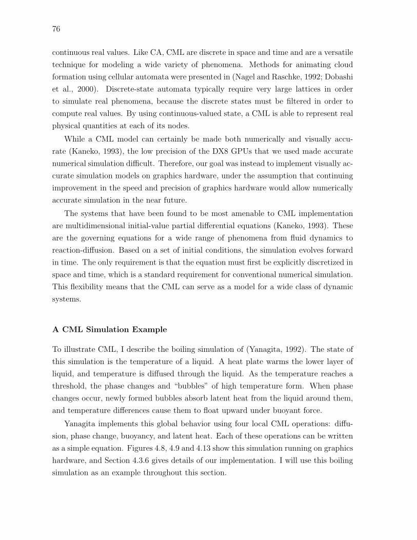
76

continuous real values. Like CA, CML are discrete in space and time and are a versatile

technique for modeling a wide variety of phenomena. Methods for animating cloud

formation using cellular automata were presented in (Nagel and Raschke, 1992; Dobashi

et al., 2000). Discrete-state automata typically require very large lattices in order

to simulate real phenomena, because the discrete states must be filtered in order to

compute real values. By using continuous-valued state, a CML is able to represent real

physical quantities at each of its nodes.

While a CML model can certainly be made both numerically and visually accu-

rate (Kaneko, 1993), the low precision of the DX8 GPUs that we used made accurate

numerical simulation difficult. Therefore, our goal was instead to implement visually ac-

curate simulation models on graphics hardware, under the assumption that continuing

improvement in the speed and precision of graphics hardware would allow numerically

accurate simulation in the near future.

The systems that have been found to be most amenable to CML implementation

are multidimensional initial-value partial differential equations (Kaneko, 1993). These

are the governing equations for a wide range of phenomena from fluid dynamics to

reaction-diffusion. Based on a set of initial conditions, the simulation evolves forward

in time. The only requirement is that the equation must first be explicitly discretized in

space and time, which is a standard requirement for conventional numerical simulation.

This flexibility means that the CML can serve as a model for a wide class of dynamic

systems.

A CML Simulation Example

To illustrate CML, I describe the boiling simulation of (Yanagita, 1992). The state of

this simulation is the temperature of a liquid. A heat plate warms the lower layer of

liquid, and temperature is diffused through the liquid. As the temperature reaches a

threshold, the phase changes and “bubbles” of high temperature form. When phase

changes occur, newly formed bubbles absorb latent heat from the liquid around them,

and temperature differences cause them to float upward under buoyant force.

Yanagita implements this global behavior using four local CML operations: diffu-

sion, phase change, buoyancy, and latent heat. Each of these operations can be written

as a simple equation. Figures 4.8, 4.9 and 4.13 show this simulation running on graphics

hardware, and Section 4.3.6 gives details of our implementation. I will use this boiling

simulation as an example throughout this section.

77

4.3.2 Common Operations

A detailed description of the implementation of the specific simulations that we modeled

using CML would require too much space, so I instead describe a few common CML

operations, followed by details of their implementation. My goal in these descriptions is

to impart a feel for the kinds of operations that can be performed on DX8 GPUs. The

example equations used in this section assume a two-dimensional lattice. Extension to

three dimensions is straightforward.

Diffusion and the Laplacian

The Laplacian, described in Section 4.2.2, appears often in the partial differential equa-

tions that describe natural phenomena. It is an isotropic measure of the second spatial

derivative of a scalar function. Intuitively, it can be used to detect regions of rapid

change, and for this reason it is commonly used for edge detection in image processing.

The Laplacian appears in all of the CML simulations that we implemented. The boiling

simulation described previously includes a thermal diffusion operation. We implement

this using an explicit form of the diffusion operator. The low precision of GeForce 3

fragment processing would cause excessive error to build up over multiple steps of an

iterative, implicit procedure. Also, because the diffusion coefficient required by the

boiling simulation is very small, instability is not a concern.

It is not possible on DX8 hardware to write a short fragment program to perform

computations such as the Laplacian. The Cg programs in Section 4.2.4 address neigh-

boring fragments by simply adding offsets to the texture coordinates. For example, the

vector coords-half2(1,0) represents the coordinates of the fragment just to the left

of the current fragment position. On DX9 GPUs, a single texture can be bound and

read multiple times using different computed texture coordinates.

To implement the same offset on a DX8 GPU, the offset must be applied before

the coordinates reach the fragment end of the pipeline. The texture coordinates of

each vertex must be offset so that the rasterized coordinates at each fragment will

also be offset. To sample one texture multiple times using different coordinates, the

same texture must be bound to multiple texture units, and different offset texture

coordinates must be provided to each texture unit. Finally, to perform the arithmetic

that combines these samples, texture blending operations must be configured to blend

the results of the multiple texture units. To say the least, programming DX8 hardware

is not straightforward.

78

Directional Forces

Most dynamic simulations involve the application of force. Like all operations in a CML

model, forces are applied via computations on the state of a node and its neighbors.

As an example, I describe a buoyancy operator used in convection and cloud formation

simulations (Miyazaki et al., 2001; Yanagita and Kaneko, 1993; Yanagita and Kaneko,

1997).

This buoyancy operator uses temperature state T to compute a buoyant velocity at

a node and add it to the node’s vertical velocity state, v:

v′i,j = vi,j +cb2

(2Ti,j − Ti+1,j − Ti−1,j) .

The subscripts represent the grid coordinates of the values. This equation expresses

that a node is buoyed upward if it is warmer than its horizontal neighbors, and pushed

downward if it is cooler. The strength of the buoyancy is controlled via the parameter

cb.

Computation on Neighbors

Sometimes an operation requires more complex computation than the arithmetic of

the simple buoyancy operation described above. The buoyancy operation of the boil-

ing simulation described in Section 4.3.1 must also account for phase change, and is

therefore more complicated:

T ′

i,j = Ti,j −cb2Ti,j [ρ(Ti,j+1)− ρ(Ti,j−1)] ,

ρ(T ) = tanh [α(T − Tc)] .

Here, cb is the buoyancy strength coefficient, α is a constant that scales the phase

change range, and ρ(T ) is an approximation of density relative to temperature, T .

The hyperbolic tangent is used to simulate the rapid change of density of a substance

around the phase change temperature, Tc. A change in density of a lattice node relative

to its vertical neighbors causes the temperature of the node to be buoyed upward or

downward. The thing to notice in this equation is that simple arithmetic will not

suffice—the hyperbolic tangent function must be applied to the temperature at the

neighbors above and below node (i, j). I discuss how to compute arbitrary functions

using dependent texturing in Section 4.3.4.

79

4.3.3 State Representation and Storage

Section 4.2.4 describes how textures are used for state field storage. On DX8 GPUs,

the frame buffer and textures are limited to storage of 8-bit unsigned integers,7 so

state values must be converted to this format before being written to texture. Physical

simulation also requires the use of signed values. Most texture storage, however, uses

unsigned fixed point values. Although fragment-level programmability available in

these GPUs uses signed arithmetic internally, the unsigned data stored in the textures

must be biased and scaled before and after processing.

4.3.4 Implementing CML Operations

An iteration of a CML simulation consists of successive application of simple operations

on the lattice. These operations consist of three steps: setup the graphics hardware

rendering state, render a single quadrilateral fit to the view port, and store the rendered

results into a texture. I refer to each of these setup-render-copy operations as a single

pass. In practice, due to limited GPU resources (for example, the number of texture

units), a CML operation may span multiple passes.

The setup portion of a pass simply sets the state of the hardware to correctly

perform the rest of the pass. Interior and boundary fragments can be processed in the

same manner as described in Section 4.2.4 for the latest GPUs.

The render-copy portion of each pass performs 4 suboperations: Neighbor Sampling,

Computation on Neighbors, New State Computation, and State Update. Figure 4.10

illustrates the mapping of the suboperations to graphics hardware. Neighbor sampling

and Computation on Neighbors are performed by the configurable texture mapping

hardware. New State Computation performs arithmetic on the results of the previous

suboperations using programmable texture blending. Finally, State Update feeds the

results of one pass to the next by rendering or copying the texture blending results to

a texture. State Update is performed using either copy to texture or render to texture,

as I described in Section 4.2.4.

Neighbor Sampling Since state is stored in textures, neighbor sampling is per-

formed by offsetting texture coordinates toward the neighbors of the texel being up-

dated. For example, to sample the four nearest neighbor nodes of node (i, j), the

7While two-channel, 16-bit textures are available on these GPUs, they do not support dynamictexture updates for this format.

80

Graphics Pipeline

Feedback

Texture Blending(Register

Combiners)

RenderTo

Texture

Vertex Program

(Set Texture Coordinates)

Texture Shaders

Texture Unit 0

Texture Unit 1

Texture Unit n

CML Operation

Iteration

SelectNeighbors

CombineSamples

(Arithmetic)

StoreNew State

Sample Neighbors

f(Neighbor 1)

f(Neighbor 2)

f(Neighbor n)

Figure 4.10: Components of a CML operation map to graphics hardware pipeline com-ponents.

texture coordinates at the corners of the quadrilateral rendered over the viewport are

offset in the direction of each neighbor by the width of a single texel. Texture co-

ordinate interpolation ensures that as rasterization proceeds, every texel’s neighbors

will be correctly sampled. Note that beyond sampling just the nearest neighbors of

a node, weighted averages of nearby nodes can be computed by exploiting the linear

texture interpolation hardware available in GPUs. Care must be taken, though, since

the precision used for the interpolation coefficients is sometimes lower than the rest of

the texture pipeline.

Computation on Neighbors As I described in Section 4.3.2, many simulations

compute complex functions of the neighbors they sample. In many cases, these func-

tions can be computed ahead of time and stored in a texture for use as a lookup table.

NVIDIA GeForce 3 and 4 GPUs provide a mechanism called texture shaders that pro-

vide a choice among many texture addressing modes for multiple texture units. ATI

Radeon 8500 provides similar functionality. I have implemented table lookups using

the DEPENDENT_GB_TEXTURE_2D_NV texture shader mode of the GeForce 3. This mode

81

T

f

[s, t]

[r, g, b]

[ f (Ts,t)]

Figure 4.11: An arbitrary function can be implemented in graphics hardware by per-forming a table lookup using dependent texturing.

provides memory indirect texture addressing—the green and blue colors read from one

texture unit are used as texture coordinates for a lookup into a second texture unit.

By binding a precomputed lookup table texture to the second texture unit, arbitrary

functions can be computed using the state of the nodes as input (See Figure 4.11).

New State Computation Once the values of neighboring texels have been sampled

and optionally used for function table lookups, the next step is to compute the new state

of the lattice. I use programmable hardware texture blending to perform arithmetic

operations including addition, multiplication, and dot products. On the GeForce 3 and

4, I implement this using register combiners (NVIDIA Corporation, 2002b). Register

combiners take the RGBA output of texture shaders and rasterization as input, and

provide arithmetic operations, user-defined constants, and temporary registers. The

result of these computations is written to the frame buffer.

4.3.5 Numerical Range of CML Simulations

The physically-based nature of CML simulations means that the ranges of state values

for different simulations can vary widely. DX8-class graphics hardware, on the other

hand, operates only on fixed point fragment values in the range [−1, 1] (and even [0, 1]

at some points). This means that we must normalize the range of a simulation into

[−1, 1] before it can be implemented in graphics hardware.

Because the hardware uses limited-precision fixed point numbers, some simulations

will be more robust to this normalization than others. The robustness of a simulation

depends on several factors. Dynamic range is the ratio between a simulation’s largest

absolute value and its smallest non-zero absolute value. If a simulation has a high dy-

namic range, it may not be robust to normalization unless the precision of computation

82

is high enough to represent the dynamic range. I refer to a simulation’s resolution as

the smallest absolute numerical difference that it must be able to discern. A simu-

lation with a required resolution finer than the resolution of the numbers used in its

computation will not be robust. Finally, as the arithmetic complexity of a simulation

increases, it will incur more roundoff error, which may reduce its robustness when using

low-precision arithmetic.

For example, the boiling simulation (Section 4.3.1) has a range of approximately

[0, 10], but its values do not get very close to zero, so its dynamic range is less than

ten. Also, its resolution is fairly coarse, since the event to which it is most sensitive—

phase change—is near the top of its range. For these reasons, boiling is fairly robust

under normalization. Reaction-diffusion has a range of [0, 1] so it does not require

normalization. Its dynamic range, however, is on the order of 105, which is much

higher than that of the 8-bit numbers stored in textures. Fortunately, by scaling the

coefficients of reaction-diffusion, we can reduce this dynamic range somewhat to get

interesting results. However, as we describe in Section 4.3.6, it suffers from precision

errors (See Section 4.3.7 for more discussion of precision issues). With the floating point

hardware available in the latest GPUs, simulations can be run within their natural

ranges.

4.3.6 Results

I designed and built an interactive framework, “CMLlab”, for constructing and exper-

imenting with CML simulations (Figure 4.12). The user constructs a simulation from

a set of general purpose operations, such as diffusion and advection, or special purpose

operations designed for specific simulations, such as the buoyancy operations described

in Section 4.3.2. Each operation processes a set of input textures and produces a single

output texture. The user connects the outputs and inputs of the selected operations

into a directed acyclic graph. An iteration of the simulation consists of traversing the

graph in depth-first fashion so that each operation is performed in order. The state

textures resulting from an iteration are used as input state for the next iteration, and

for displaying the simulated system. The results of intermediate passes in a simulation

iteration can be displayed to the user in place of the result textures. This is useful for

visually debugging the operation of a new simulation.

While 2D simulations in our framework use only 2D textures for storage of lattice

state, 3D simulations can be implemented in two ways. The obvious way is to use 3D

83

Figure 4.12: CMLlab, my interactive framework for building and experimenting withCML simulations. CMLlab provides the ability to connect various CML operationsto generate unique simulations. This image shows a 2D reaction-diffusion simulationrunning in the CMLlab application window.

Figure 4.13: A 3D CML boiling simulation running in an interactive environment (thesteam is a particle system).

84

Figure 4.14: A 2D CML simulation of Rayleigh-Benard convection. The left panelshows temperature; the right panel shows 2D velocity encoded in the blue and greencolor channels.

Figure 4.15: A sequence from a 3D version of the Gray-Scott reaction-diffusion model.

85

textures. However, the extra overhead of copying from the frame buffer to each slice

of a 3D texture can make simulations run much slower. Instead, we implemented 3D

simulations using a collection of 2D textures that represent slabs of the 3D volume.

While this is faster than updating a 3D texture, it has disadvantages. For example, we

cannot take advantage of the built in trilinear filtering and texture boundaries (clamp

or repeat) that are provided in hardware for 3D textures. In the next chapter, I describe

a method of using a single 2D texture to represent a 3D grid.

It is worth noting that we trade optimal performance for flexibility in the CMLLab

framework. Because we want to allow a variety of models to be built from a set of

operations, we often incur the expense of some extra texture copies in order to keep

operations separate. Thus, our implementation is not optimal - even faster rates are

achievable on the same hardware by sacrificing operator reuse.

To demonstrate the utility of hardware CML simulation in interactive 3D graphics

applications, we integrated the simulation system into a virtual environment built on

a 3D game engine, “Wild Magic” (Eberly, 2001). Figure 4.13 is an image of a boiling

witch’s brew captured from a real-time demo we built with the engine. The demo

uses our 3D boiling simulation (Section 4.3.6) and runs at 45 frames per second on an

NVIDIA GeForce 4.

In the following sections I describe three of the CML simulations that we imple-

mented. The test computer I used was a PC with a single 2.0 GHz Pentium 4 processor

and 512 MB of RAM. Tests were performed on this machine with both an NVIDIA

GeForce 3 Ti 500 GPU with 64 MB of RAM, and an NVIDIA GeForce 4 Ti 4600 GPU

with 128 MB of RAM.

Boiling

I implemented 2D and 3D boiling simulations as described in (Yanagita, 1992). Rather

than simulate all components of the boiling phenomenon (temperature, pressure, veloc-

ity, phase of matter, surface tension, etc.), their model simulates only the temperature

of the liquid as it boils. The simulation is composed of successive application of ther-

mal diffusion, bubble formation and buoyancy, and latent heat transfer operations. The

first two of these are described in Section 4.3.2, and Section 4.3.1 gives an overview

of the model. For details of the latent heat transfer computation, I refer the reader

to (Yanagita, 1992). Our implementation requires seven passes per iteration for the

2D simulation, and 9 passes per slice for the 3D simulation. Table 4.3.6 shows the

simulation speed for a range of resolutions. For details of my boiling simulation imple-

86

Iterations Per Second SpeedupResolution Software GeForce 3 GeForce 4 GeForce 3 GeForce 4

64× 64 266.5 1252.9 1752.5 4.7 6.6128× 128 61.8 679.0 926.6 11.0 15.0256× 256 13.9 221.3 286.6 15.9 20.6512× 512 3.3 61.2 82.3 18.5 24.9

1024× 1024 0.9 15.5 21.6 17.2 2432× 32× 32 25.5 104.3 145.8 4.1 5.764× 64× 64 3.2 37.2 61.8 11.6 19.3

128× 128× 128 0.4 NA 8.3 NA 20.8

Table 4.2: A speed comparison of a hardware CML boiling simulation to a softwareversion. “NA” means that the simulation was not performed on GeForce 3 due tomemory size limitations.

mentation, see (Harris, 2002b).

Convection

The Rayleigh-Benard convection CML model of (Yanagita and Kaneko, 1993) simulates

convection using four CML operations: buoyancy (Section 4.3.2), thermal diffusion

(Section 4.3.2, temperature and velocity advection, and viscosity and pressure effect.

The viscosity and pressure effect is implemented as8

~u′ = ~u+kv

4∇2~u+ kp∇(∇· ~u),

where ~u is the velocity, kv is the viscosity and kp is the coefficient of the “pressure

effect” (Yanagita and Kaneko, 1993). The first two terms of this equation account for

viscous diffusion of the velocity, and the last term is the flow caused by the gradient of

the mass flow around the lattice (Miyazaki et al., 2001). This operation is an ad hoc

simplification of the viscous diffusion and projection operations used in fluid simulation

(See Section 4.2). Details of the discrete implementation of this operation are available

in (Yanagita and Kaneko, 1993; Miyazaki et al., 2001).

The remaining operation is advection of temperature and velocity by the velocity

field. Yanagita and Kaneko implement this using an explicit method that distributes

state from a node to its neighbors according to the velocity at the node. As I noted in

Section 4.2.3, this is not possible on current graphics hardware because the fragment

8Clearly the last term in this equation should be ∇·∇~u, but (Yanagita and Kaneko, 1993) chosethis formulation. Their reasoning is unclear.

87

processors cannot perform random access writes. Instead, I used an implicit method

like the one described previously. In order to implement this technique on DX8-class

hardware, I used a texture shader-based advection operation. This operation advects

state stored in a texture using the GL_OFFSET_TEXTURE_2D_NV dependent texture ad-

dressing mode of the GeForce 3 and 4. A description of this method of advection can

be found in (Weiskopf et al., 2001). My 2D convection implementation (Figure 4.14)

requires 10 passes per iteration. I did not implemented a 3D convection simulation

because GeForce 3 and 4 do not have a 3D equivalent of the offset texture operation.

Due to the precision limitations of the graphics hardware, my implementation of

convection did not behave exactly as described in (Yanagita and Kaneko, 1993). I do

observe the formation of convective rolls, but the motion the flow is quite turbulent. I

believe that this is a result of low-precision arithmetic.

Reaction-Diffusion

Reaction-diffusion processes were proposed in (Turing, 1952) and introduced to com-

puter graphics by (Turk, 1991; Witkin and Kass, 1991). They are a well-studied model

for the interaction of chemical reactants, and are interesting due to their complex and of-

ten chaotic behavior. The patterns that emerge are reminiscent of patterns occurring in

nature (Lee et al., 1993). Using our CMLlab environment, Greg Coombe implemented

the Gray-Scott reaction-diffusion model (Pearson, 1993). This is a two-chemical system

defined by the following initial value partial differential equations.

∂U

∂t= Du∇

2U − UV 2 + F (1− U)

∂V

∂t= Dv∇

2V + UV 2 − (F + k)V

Here F , k, Du, and Dv are parameters given in (Pearson, 1993). Greg implemented 2D

and 3D versions of this process, as shown in Figure 4.12 (2D), and Figures 4.8 and 4.15

(3D). Reaction-diffusion was relatively simple to implement in our framework because

we were able to reuse the existing diffusion operator. In 2D this simulation requires two

passes per iteration, and in 3D it requires three passes per slice. A 256x256 lattice runs

at 400 iterations per second in our interactive framework, and a 128x128x32 lattice

runs at 60 iterations per second.

The low precision of DX8 GPUs reduces the variety of patterns that the Gray-

Scott model produces. We have seen a variety of results, but much less diversity than

88

produced by a floating point implementation. As with convection, this is caused by the

effects of low-precision arithmetic.

4.3.7 Discussion of Precision Limitations

The low-precision of the fragment processors on DX8 GPUs limits their usefulness

for physically-based simulation. The register combiners in the GeForce 3 and 4 per-

form arithmetic using nine-bit signed fixed point values. Without floating point, the

programmer must scale and bias values to maintain them in ranges that maximize pre-

cision. This is not only difficult, it is also subject to arithmetic error. Some simulations

(such as boiling) handle this error well, and behave as predicted by a floating point

implementation. Others, such as reaction-diffusion, are more sensitive to precision

errors.

I analyzed the error introduced by low precision and did some experiments to de-

termine how much precision is needed for the reaction-diffusion implementation (For

full details, see (Harris, 2002a)). I hypothesize that the diffusion operation is very sus-

ceptible to roundoff error, because in my experiments in CMLlab, iterated application

of a diffusion operator never fully diffuses its input. I derived the error εd induced by

each application of diffusion (in 2D) to a node (i, j) as

εd ≈ ε(3 +3d

4+ xi,j)

where d is the diffusion coefficient, xi,j is the value at node (i, j), and ε is the amount

of roundoff error in each arithmetic operation. Since d and xi,j are in the range [0, 1],

this error has an upper bound of |εd| ≤ 4.75ε. With 8 bits of precision, ε is at most 2−9.

This error is fairly large, meaning that a simulation that is sensitive to small numbers

will quickly diverge.

In an attempt to better understand the precision needs of more sensitive simulations,

we implemented a software version of the reaction-diffusion simulation with adjustable

fixed point precision. Through experimentation, we found that with 14 or more bits

of fixed point precision, the behavior of this simulation is visually very similar to a

single-precision floating point implementation. Like the floating point version, a diverse

variety of patterns grow, evolve, and sometimes develop unstable formations that never

cease to change. Figure 4.16 shows a variety of patterns generated with this 14-bit

fixed point simulation.

Upon the release of the NVIDIA GeForce FX, I verified that a floating point GPU

89

Figure 4.16: The result of the 2D gray-scott reaction diffusion with varying parameters.By varying the fixed-point computation precision we determined that 14 bits of precisionwere sufficient to approximate the results of a 32-bit floating point simulation. Withthe advent of floating point GPUs, this is no longer necessary (see Section 4.3.7).

implementation of the Gray-Scott reaction diffusion model can generate the same rich

variety of patterns as a software implementation. This model is implemented using

a single Cg fragment program. I demonstrated the use of reaction-diffusion as a pat-

tern generator for making frightening bump-mapped “disease” spots appear on a 3D

character model, as shown in Figure 4.17 (Harris and James, 2003).

4.4 Summary

I began this chapter with a discussion of the trend that I call General-Purpose Com-

putation on GPUs (GPGPU) and categorized GPUs according to the version of the

DirectX API that they support. For completeness, the last part of the chapter (Section

4.3), describes simulation of coupled map lattice models and simple PDEs on lower-

precision DX8-class GPUs. The most important part of this chapter is Section 4.2, in

which I explain the “Stable Fluids” algorithm for fluid simulation, and a method for

implementing it on the GPU. This technique is the core on which I build my GPU

cloud simulation in the next chapter.

90

Figure 4.17: This image demonstrates a 2D Gray-Scott reaction-diffusion simulationrunning on an NVIDIA GeForce FX GPU. The results of the simulation are convertedinto bump and color maps used to create creepy moving ”disease” spots.

Chapter 5

Simulation of Cloud Dynamics

Clouds can form in many ways. Convective clouds form when moist air is warmed and

becomes buoyant. The air rises, carrying water vapor with it, expanding and cooling as

it goes. As the temperature and pressure of the air decrease, its saturation point—the

equilibrium level of evaporation and condensation—is reduced. When the water vapor

content of the rising air becomes greater than its saturation point, condensation occurs,

which yields the microscopic condensed cloud water particles that we see as clouds in

the sky. Condensation increases the drag on the air, causing it to slow its ascent, which

creates a natural limit on the vertical extent of a cloud layer. Stratus clouds usually

form when masses of warm and cool air mix due to radiative cooling or lifting of the

air over terrain (Orographic lifting). An example of the formation of stratus clouds by

mixing is the fog that often rolls into the city of San Francisco.

I have developed a cloud dynamics simulation based on partial differential equations

that model fluid flow, thermodynamics, and water condensation and evaporation, as

well as various forces and other factors that influence these equations. These equations

are described in detail in Chapter 2. Aided by Bill Baxter and Thorsten Scheuermann,

I implemented the discrete form of these equations using programmable floating-point

graphics hardware (Harris et al., 2003). All computation and rendering is performed

on the GPU; the CPU provides only high-level control. In this chapter I describe

the implementation of the simulation in detail, along with two useful optimizations: a

representation of volume data in two-dimensional textures, and an efficient packing of

scalar fields to best exploit the vector operations of the fragment processor. Figure 5.1

shows a sequence from a two-dimensional cloud simulation, and Figures 1.2 and 5.4

show 3D clouds.

In order to incorporate dynamic 3D clouds into interactive graphics applications,

92

the per-frame simulation cost must be small enough that it does not interfere with

the application. In Section 5.5 I describe a method for amortizing the simulation cost

over multiple frames, allowing the application to budget time for the simulation in each

frame. This technique greatly improves interactivity, allowing a user to view the results

of a simulation at 60 frames per second or higher while the simulation progresses at

several iterations per second. I integrated cloud simulation with an interactive flight

application (Harris and Lastra, 2001) that reduces the high cost of slice-based volume

cloud rendering by using dynamically-generated impostors. I describe algorithms for

efficient rendering of illuminated clouds in Chapter 6.

5.1 Solving the Dynamics Equations

As I described in Chapter 2, my simulation solves the Euler equations of incompressible

fluid flow, (2.3) and (2.4), the water continuity equation, (2.14), and the thermodynamic

equation, (2.18).

5.1.1 Fluid Flow

My cloud model is based on the equations of fluid flow, so my simulator is built on top

of a standard fluid simulator much like the ones described by (Stam, 1999; Fedkiw et al.,

2001). It solves the equations of motion using the stable two step technique described

in those papers and detailed in Chapter 4. In the first step, I use the semi-Lagrangian

advection technique that Stam described to compute an intermediate velocity field ~u′,

and add to it the buoyancy force, Equation (2.10), and vorticity confinement force,

Equation (4.17). This step solves Equation (2.3) without the pressure term. In the

second step, the intermediate field ~u′ is made incompressible (so that it satisfies both

Equation (2.3) and Equation (2.4)) using the Helmholtz-Hodge decomposition (see

Section 4.2.3).

Using the advection technique as for velocity, I also advect the potential tempera-

ture, θ, and water variables, qv and qc. During advection, I apply different boundary

conditions for each of the variables. For the velocity, I use the no-slip condition (~u = 0)

on the bottom boundary, and free-slip condition (∂~u/∂n = 0) on the top. At the sides,

I set the horizontal velocities to the user-defined horizontal wind speeds. I set the

top and side temperature boundaries to the user-defined ambient temperature. I use

periodic side boundaries for qv to simulate water vapor being blown in from outside

93

Figure 5.1: A sequence of stills (left-to-right, top-to-bottom) from my 2D cloud simu-lation, running on a 128x128 grid at greater than 30 frames per second.

the simulation domain, and I set all qc boundaries and the top qv boundary to zero.

Finally, I specify input fields at the bottom boundary for both temperature and water

vapor. These fields are randomly perturbed, user-specified constant values, and are the

source of the temperature and water that cause clouds to form.

5.1.2 Water Continuity

The solution of the water continuity equations (2.14) is straightforward. The equations

state that the changes in qv and qc are governed by advection of the quantities as

well as by the amount of condensation and evaporation. I solve them in two steps.

First, I advect each using the semi-Lagrangian technique mentioned before, resulting

in intermediate values q′v and q′c. Then, at each cell, I compute the new mixing ratios

as follows:∆q′v = −∆C = min(qvs − q

′

v, q′

c),

qv = q′v + ∆q′v,

qc = q′c −∆q′v,

(5.1)

where ∆C is the amount of condensation over the time step, and qvs is computed using

equation (2.13) as described in Section 2.1.7. I compute T using equation (2.9) with

the current potential temperature θ, and the local environmental pressure computed

with equation (2.11).

5.1.3 Thermodynamics

The left-hand side of the thermodynamic equation, (2.18), shows that like the other

quantities, potential temperature is advected by the velocity field, so I compute an

94

intermediate value, θ′ via the semi-Lagrangian advection scheme. As mentioned in

Section 2.1.8, I substitute −C for the quantity in parentheses on the right-hand side

of the thermodynamic equation. This means that the temperature increases by an

amount proportional to the amount of condensation, and I update it as follows:

θ = θ′ +L

cpΠ∆C. (5.2)

5.2 Implementation

I solve the cloud dynamics equations on a grid of voxels. I use a staggered grid dis-

cretization of the velocity and pressure equations as in (Foster and Metaxas, 1997;

Griebel et al., 1998; Fedkiw et al., 2001). This means that pressure, temperature, and

water content are defined at the center of voxels while velocity is defined on the faces

of the voxels. Not only does this method reduce numerical dissipation as mentioned by

Fedkiw et al., but as Griebel et al. explain, it prevents possible pressure oscillations

that can arise with collocated grids (in which all variables are defined at cell centers).

My experiments with collocated grids have indeed shown some undesirable pressure

oscillations when buoyant forces are applied. Section 5.4 describes my implementation

of voxel grids using textures.

Overall, my algorithm for solving the equations of cloud dynamics at each discrete

time step is as follows.

1. Advect θ, qv, qc and velocity, ~u.

2. Compute vorticity confinement force, ~fvc.

3. Compute buoyant force, Bk.

4. Compute ~u′ = ~uadvected + (Bk + ~fvc)δt.

5. Update qv and qc according to Equation (5.1).

6. Update θ according to Equation (5.2).

7. Compute the divergence ∇· ~u′.

8. Solve the Poisson-pressure equation, (4.6).

9. Compute ~u = ~u′ −∇p.

My implementation of steps 1, 2, 7, and 9 follows (Fedkiw et al., 2001) nearly

exactly. I refer the reader to the appendix of that paper for the discrete form of the

equations. Step 3 can be implemented directly from equation (2.10). However, I find

that providing the user with a scale factor applied to qH provides useful control over

95

the buoyancy of clouds. In my implementation, steps 5 and 6 are performed in a single

fragment program, because I store the water and temperature variables in a single

texture. For the same reason, I advect the potential temperature and water variables

simultaneously. I solve the remaining step, the Poisson-pressure equation, using a

standard iterative relaxation solver applied to equation (4.6).

Fedkiw, et al. use the conjugate gradient method with an incomplete Choleski

preconditioner to solve the Poisson-pressure equation (Fedkiw et al., 2001). While

this is a straightforward solver to implement and run on a CPU, my implementation

uses fragment programs that run on the GPU. Implementation of conjugate gradient

on the GPU is feasible (Bolz et al., 2003; Kruger and Westermann, 2003), but many

passes are required just to compute the large vector inner products required by the

algorithm (O(log2N) passes, where N is the grid resolution). For this reason, I chose

to use a simple solver such as Jacobi or Red-Black Gauss Seidel relaxation (Golub and

Van Loan, 1996). These solvers can be implemented to run in one and two render

passes, respectively, using only a few lines of Cg code. Therefore I can run more

iterations in a given amount of time than with a more complex method, which helps

make up for the slower convergence of the chosen solver. Section 5.4.1 discusses the

efficient implementation of these solvers.

I typically use a grid scale (δx) of 50–100 m. I choose an altitude range, and then

set the grid scale so that the grid covers that range. For example, if I want to represent

a 3.2 km altitude range1, then I set δx to 100 m on a 32× 32 × 32 grid, or 50 m on a

64× 64× 64 grid.

5.3 Hardware Implementation

As I mentioned before, the cloud simulator performs all numerical computation in the

programmable, floating point fragment unit of a graphics processor. State fields, such as

p and ~u, are stored in textures. For efficiency, I store θ, qv, and qc in different channels

of the same texture. Computation is performed as described in Chapter 4. State

textures are updated using a render pass that draws a quadrilateral fit to the viewport.

I implement computations using fragment programs written in the Cg shading language

(Mark et al., ). The fragment programs implement the steps described in Section 5.2

using texturing operations to read data from the grids. At the end of a render pass,

the state texture is updated as described in Section 4.2.4.

1The base of cumulus clouds is typically 1–2 km in fair, humid weather (Rogers and Yau, 1989).

96

3D Texture Corresponding Flat 3D Texture01234567

0 1 2 3

7654

quad primitives line primitives

NN

Figure 5.2: A Flat 3D Texture is a 2D texture made up of the tiled slices of a 3D texure.Flat 3D Textures allow all slices of the volume to be updated in a single rendering pass.

5.4 Flat 3D Textures

Section 4.3.6 describes how I used stacks of 2D textures to represent 3D volumes on

DX8 GPUs, because of the expense of updating a 3D texture. To apply a simulation

operation to the grid—for example to compute the buoyancy force—the volume must

be updated slice by slice. At each slice, the operation is applied, and the texture for that

slice is updated, requiring a texture copy or a context switch associated with render to

texture.

On DX9 GPUs, it is possible to avoid the overhead of a texture update per volume

slice. For cloud simulation, I represent grids using what I call a “flat” 3D texture. A

flat 3D texture is a 2D texture that contains the tiled slices of a 3D volume, as shown

in Figure 5.2. In the figure, the white borders represent the boundary cells of each

slice, and the white boxes in the lower left and upper right represent the boundary

slices on the ends of the volume along the slicing axis. Updating a flat 3D texture is

much like the 2D texture update described in the previous section. I render the interior

of each slice (the gray squares) using a quad primitive, and I render the boundaries

using line primitives. I use one fragment program for all of the interior quad primitives,

and another for the boundary lines and the two “end cap” (lower left and upper right)

quads.

The advantage of true 3D textures over flat 3D textures is that addressing them is

easy, since the GPU supports it. With flat 3D textures, however, the r (depth) texture

97

coordinate must be converted into a 2D offset in each fragment program in order to

do a texture lookup. In practice, I precompute a 1D lookup texture that contains the

offsets for each slice, and use this as an indirection table indexed by the r coordinate.

Flat 3D textures can be updated in a single render pass—only one texture update

is required for the entire volume. This means that a 3D simulation can be implemented

in the same number of passes as an equivalent 2D simulation (ignoring changes in the

computation itself). Flat 3D textures provide a performance advantage over true 3D

textures on current hardware. While the amount of data copied or updated is the

same, in my experience, the total slice update overhead is much greater for true 3D

textures. Also, because more fragments are processed in a single pass, flat 3D textures

make better use of the parallelism of the fragment processor. Finally, flat 3D textures

provide a quick, inexpensive way to preview the results of a 3D simulation, since they

can be easily rendered as a 2D image.

5.4.1 Vectorized Iterative Solvers

Iterative solution of the Poisson equation for pressure is one of the most expensive

operations in numerical fluid and cloud simulation. For simulation on the GPU, the

choice of solver is limited by the inability of fragment programs to both read and

write the same memory in the same pass. This rules out Gauss-Seidel and Successive

Over-relaxation (SOR), which have been used in many previous graphics applications

of fluid simulation. Bill Baxter and I have, however, implemented several solvers and

conducted an investigation to determine the most efficient of these given the constraints

of graphics hardware. The results are given in Table 5.1.

Our Jacobi solver stores pressure as a single-channel floating point texture. The

Jacobi fragment program also takes a divergence texture as input, and computes an

updated pressure value as output for each fragment by sampling neighboring pressure

values and subtracting the input divergence. After this single pass the output texture

is used as input for the next iteration of the solver.

Red-Black Gauss-Seidel is a variation on Jacobi that splits the cells into two sets

such that new Red cell values only depend on Black cell inputs, and vice versa (see

Figure 5.3). All the Red values can be updated using only the old Black values, and

then the Black values can be updated using the new Red values. Using the most

recently-updated half of the cells for updates improves the convergence rate.

To implement Red-Black efficiently we pack four pressure values into a single RGBA

98

g g gi-1,j i,j i+1,j

gi,j+1

gi,j

gi,j-1

VectorizedRed-Black Grid

= Black Cells

= Red Cells

= Unused boundary cells

= A vectorized texel(rgba = color mapping)

,

r gba

Figure 5.3: Efficient iterative Poisson solvers can be implemented by packing multiplescalar values into each texel. The cross pattern demonstrates the sampling pattern forvectorized Jacobi and Red-Black iteration.

Figure 5.4: Simulated clouds in the SkyWorks interactive flight application.

99

Poisson Solver Convergence per msa Convergenceb Timec (ms)

Jacobi 2D 0.50 0.078 45.9

Red-Black 2D 0.85 0.124 45.3

Vectorized Jacobi 2D 1.0 0.079 17.3

Jacobi 3D NC NC 110d

Vectorized Jacobi 3D NC NC 49.0

a Normalized convergence per millisecond achieved with a 17 ms time budget.b Relative convergence after 100 iterations.c Time for execution of 100 iterations.d Estimated from register usage, program length, and fragment count for 3D Jacobi

program.

Table 5.1: A comparison of the convergence rates of various iterative solversrunning on the GPU. All grids were 128× 128 or 32× 32× 16. (NC ≡ “NotComputed”.)

texel, as shown in Figure 5.3. This allows us to reduce the overall number of texture

lookups required for each half-pass of Red-Black. Without packing, the Red pass would

require 5 texture lookups per pressure update (corresponding to the 5 cells of a 5-point

discrete Laplacian) in 2D, and 7 lookups in 3D. By packing pressure in a vectorized

format the same 5 or 7 texture lookups enable us to update 4 pressure values instead

of just one, as can been seen in Figure 5.3. With the 5 samples shown, the 4 pressure

values in gi,j can be updated. This is a significant savings; however, we incur extra

overhead since the Black cells must be explicitly passed through on a Red pass and

vice versa, so that both Red and Black are written every pass, and we also incur the

overhead of two rendering passes for one solver iteration. Still, Red-Black converges

faster than a basic Jacobi solver given a fixed time budget.

The same vectorization technique used to accelerate the Red-Black solver can also

be used to accelerate the Jacobi solver. With vectorization, two full Jacobi iterations

take less time than a full Red-Black iteration, and give better convergence. The result

is that vectorized Jacobi gives the best convergence under a fixed time budget of any

of the hardware solvers we tested (See Table 5.1).

100

5.5 Interactive Applications

Cloud simulation is a computationally intensive process that is usually done offline. But

simulations of phenomena such as clouds have the potential to provide rich dynamic

content for interactive applications, so one of my goals has been to create a simulation

that will work well online.

As a test of this, I integrated cloud simulation into my cloud rendering engine,

SkyWorks (Harris and Lastra, 2001). SkyWorks was designed to render scenes full of

static clouds very fast. As I describe in Chapter 6, it precomputes the illumination of

the clouds, and then uses this illumination to render the clouds at run time. To reduce

the cost of rendering the clouds, it uses dynamically generated impostors (Schaufler,

1995).

5.5.1 Simulation Amortization

Real-time visualization of simulated 3D clouds requires that the per-frame simulation

cost be small enough that it does not interfere with the application. If I were to perform

a complete simulation time step every frame, the application’s frame rate would drop

below the frame rate of the cloud simulation. As an example, a simulation on a grid of

resolution 643 updates at under four iterations per second. This is not an acceptable

frame rate for a flight simulator.

To avoid this problem, we (Bill Baxter and I) built into the simulation system a

method for automatically dividing the work of a simulation time step over multiple

frames. This is fairly straightforward to do with a GPU simulation because each oper-

ation is a render pass. We instrumented our simulator with the ability to measure the

time taken by any render pass. Every so often (usually just at startup and at the user’s

request) we run a complete simulation step with these timers active, and we record the

time for each step. Then, in each frame of the application, the application budgets

a certain amount of time for the simulation, and the simulator attempts to stay as

close to that budget as possible by executing just as many passes as will fit in the time

budget.

This technique makes a tremendous difference in the performance of application.

In SkyWorks, the user can fly around and through dynamic clouds at 40-80 frames per

second while the simulation updates 1-5 times per second. Since the simulation time

step can be set at a few seconds (thanks to the stable fluid simulation), clouds can

update in approximately “real time”.

101

Iterations Per Second

Resolution P4a Quadro FXb GeForce FX 5800c GeForce FX 5900d

16× 16 518.67 368.32 585.48 642.67

32× 32 239.64 364.30 583.09 620.35

64× 64 73.38 164.37 256.34 289.18

128× 128 16.59 49.01 74.44 89.49

256× 256 3.84 13.03 19.22 21.35

512× 512 0.98 3.29 4.82 5.22

1024× 1024 0.25 0.69 1.02 1.28

a Intel Pentium 4 2.0 GHz CPU w/ 512 MB RAM.b NVIDIA Quadro FX 1000 GPU w/ 128 MB RAM.c NVIDIA GeForce FX 5800 Ultra GPU w/ 128 MB RAM.d NVIDIA GeForce FX 5900 Ultra GPU w/ 256 MB RAM.

Table 5.2: Performance data for two-dimensional cloud simulation on a CPUand three different GPUs.

Still, this system is not perfect, because it is very difficult to accurately time an

operation in the graphics pipeline. In order to get the best interactivity, the simulator

must only rarely go over budget. To ensure this, we try to get worst case timings for

each operation by forcing the pipeline to flush before stopping the timer. But this

is not realistic, because under normal conditions (i.e. without forced flushes) there

is more parallelism in the GPU. Therefore, a better method—perhaps with hardware

support—of timing GPU operations would be useful.

5.6 Results

My GPU simulation system enables fast, physically-based cloud simulation on larger

volumes than have been used previously in computer graphics applications. On volumes

of resolution 32 × 32 × 32 and 64 × 64 × 64, the simulator achieves update rates of

approximately 27.4 and 3.9 iterations per second, respectively, on an NVIDIA GeForce

FX 5900 Ultra. Tables 5.2 and 5.3 provide detailed performance data (in iterations per

second) for two- and three-dimensional cloud simulation at a variety of resolutions. I

ran the simulations on an Intel Pentium 4 CPU with 512MB of RAM and on three

different NVIDIA GPUs: a Quadro FX 1000 with 128MB of RAM, a GeForce FX 5800

102

Iterations Per Second

Resolution P4a Quadro FXb GeForce FX 5800c GeForce FX 5900d

16× 16× 16 49.55 34.84 82.64 69.54

32× 32× 32 5.13 16.02 24.44 27.43

64× 64× 64 0.57 2.20 3.36 3.87

128× 128× 32 0.24 1.01 1.47 2.08

128× 128× 64 0.12 0.48 0.71 1.02

128× 128× 128 0.07 NCe NCe 0.37

a Intel Pentium 4 2.0 GHz CPU w/ 512 MB RAM.b NVIDIA Quadro FX 1000 GPU w/ 128 MB RAM.c NVIDIA GeForce FX 5800 Ultra GPU w/ 128 MB RAM.d NVIDIA GeForce FX 5900 Ultra GPU w/ 256 MB RAM.e Not computed due to memory size limitations.

Table 5.3: Performance data for three-dimensional cloud simulation on a CPU andthree different GPUs. Two of the GPUs had only 128 MB of RAM, and thereforecould run a maximum simulation size of 128×128×64. The other GPU had 256MBof RAM, and could run a maximum simulation size of 128× 128× 128.

Ultra with 128MB of RAM, and a GeForce FX 5900 Ultra with 256MB of RAM.

Figures 5.5 and 5.6 show the relative performance of the simulations on the four

different processors. The figures show that in all tests, GPU simulations outperformed

the CPU simulation. In the bar charts, the speedup of each simulation over the CPU

simulation is printed at the end of the bar representing the speed of the simulation

in iterations per second. At the lowest-resolution, the CPU slightly outperforms the

slowest GPU, but the resolution is so low as to not be of practical use. The maximum

speedup attained was 5.6 in 2D, and 8.7 in 3D, both on the GeForce FX 5900 Ultra.

Note that I was unable to run some of the highest-resolution 3D simulations on all

GPUs. This is because of the data size of the simulations. A single 128×128×128 grid

requires 32MB of storage (because each grid cell holds 4 32-bit values). My simulator

requires at least 4 of these grids to store the state and temporary values, plus auxiliary

rendering buffers. Therefore, the largest simulation possible on GPUs with only 128MB

of RAM is 128× 128× 64. The GeForce FX 5900 Ultra GPU with 256MB of RAM is

able to execute a 128× 128× 128. simulation.

Simulation amortization has proven very valuable for visualizing the results of simu-

lations. Combined with my efficient illumination algorithm and the use of impostors for

103

Average time per pass (ms)

Advected Quantity Colocated Grid Staggered Grid

Scalar 2D 0.71 0.87

Velocity 2D 0.67 2.40

Total 2D 1.39 3.28

Scalar 3D NC 2.34

Velocity 3D NC 8.28

Total 3D NC 10.61

Split Velocity 3D (3 passes) NC 5.90

Total 3D with Split Velocity NC 8.24

Table 5.4: Cost comparison for various implementations of theadvection operation. (NC ≡ “not computed”.)

rendering (see Chapter 6), this technique allows the user to move around and through

clouds like the ones in Figures 1.2 and 5.4 at high frame rates (the grid resolutions in

these figures are 64× 32× 32 and 64× 32× 64, respectively).

The advection portion of the simulation is one of its bottlenecks. This is especially

true in the case of staggered grid advection. Bill Baxter and I compared the performance

of advection under various conditions, shown in Table 5.4. We found that in large 3D

staggered grid simulations, the advection step could cause a large, regular jump in the

otherwise smooth frame rate when performing amortized simulation. We solved this

problem by splitting advection into three less expensive passes (one for each dimension).

This increase in granularity enables a more balanced per-frame simulation cost, since

the velocity computation can be spread over more than one frame.

Because velocity is stored in three separate color channels of a texture, we use the

color mask functionality of OpenGL to ensure that each advection pass writes only

a single color channel. This way, only one texture update is necessary for all three

passes. Splitting advection has another advantage. Fragment program performance

on GeForce FX decreases with the number of registers used. Therefore even though

the total instruction count for the split version is slightly higher, the shorter fragment

programs execute faster because they use fewer registers. Therefore the total cost of

split advection is lower, as shown in Table 5.4.

104

5.7 Summary

This chapter describes my cloud simulation system. My simulation algorithm uses the

GPU to solve the dynamics equations (Section 5.1). In order to improve performance

on 3D simulations, I use flat 3D textures, which allow the entire volume to be updated

in a single pass (Section 5.4). I improve performance on the most intensive step of

the simulation—solving the Poisson-pressure equation—by using a vectorized iterative

solver that packs four scalar values into each color channel of a texture in order to reduce

computation (Section 5.4.1). To enable integration of my simulation with interactive

applications such as flight simulators, I use a technique called simulation amortization

(Section 5.5). This spreads the computation of each simulation time step over multiple

frames, so that the rendering frame rate remains high and relatively consistent. The

result of these components is a fast cloud dynamics simulation that produces realistic

clouds in real time. In the next chapter I discuss techniques for illuminating and

rendering these clouds.

105

0 10 100 1000

16 x 16

32 x 32

64 x 64

128 x 128

256 x 256

512 x 512

1024 x 1024

1.21.1

0.71.0

2.62.4

1.51.0

3.93.5

2.21.0

5.44.5

3.01.0

5.65.0

3.41.0

5.34.9

3.31.0

5.24.2

2.81.0

Sim

ulat

ion

Grid

Res

olut

ion

Simulation Iterations Per Second (log scale)

2D Cloud Simulation Performance Comparison

Values to the right of bars representspeedup over pentium 4.

NVIDIA GeForce FX 5900 Ultra (256 MB)NVIDIA GeForce FX 5800 Ultra (128 MB)NVIDIA Quadro FX 1000 (128 MB)Intel Pentium 4 2GHz (512 MB)

Figure 5.5: A comparison of two-dimensional cloud simulation performance on variousGPUs and a CPU. The lengths of the bars represent the execution speed, in iterationsper second, of the simulation running on each processor at a variety of resolutions.For comparison, the speedup each processor achieves over a 2 GHz Pentium 4 CPU isprinted at the end of each bar. In these tests, the Jacobi solver was run for 40 iterationsat each time step.

106

0 10 100

16x16x16

32x32x32

64x64x64

128x128x32

128x128x64

128x128x128

1.41.7

0.71.0

5.34.8

3.11.0

6.85.9

3.91.0

8.66.1

4.11.0

8.76.0

4.11.0

5.70.00.0

1.0

Sim

ulat

ion

Grid

Res

olut

ion

Simulation Iterations Per Second (log scale)

3D Cloud Simulation Performance Comparison

Values to the right of bars representspeedup over pentium 4.

NVIDIA GeForce FX 5900 Ultra (256 MB)NVIDIA GeForce FX 5800 Ultra (128 MB)NVIDIA Quadro FX 1000 (128 MB)Intel Pentium 4 2GHz (512 MB)

Figure 5.6: A comparison of three-dimensional cloud simulation performance on variousGPUs and a CPU. The lengths of the bars represent the execution speed, in iterationsper second, of the simulation running on each processor at a variety of resolutions.For comparison, the speedup each processor achieves over a 2 GHz Pentium 4 CPU isprinted at the end of each bar. The highest resolution simulation was not run on theGPUs with only 128 MB of RAM because the simulation data would not fit in memory.In these tests, the Jacobi solver was run for 40 iterations at each time step.

Chapter 6

Cloud Illumination and Rendering

Chapters 2 through 5 provide detailed information about simulating cloud dynamics

using graphics hardware. In order to create beautiful and realistic images from these

simulations, I must simulate another aspect of cloud physics—cloud radiometry. Volu-

metric clouds are expensive to render, and generating images fast enough for interactive

applications is difficult. In this chapter I describe algorithms for simulating cloud ra-

diometry and a method for accelerating cloud rendering using dynamically generated

impostors.

6.1 Cloud Illumination Algorithms

In Section 2.2, I defined the essential radiometry terms necessary to simulate the in-

teraction of light with clouds. From these basics, in this section I derive simplified

equations and present algorithms for computing the illumination of clouds. In the pre-

vious two chapters, I described techniques for simulating the dynamics of clouds. The

result of the simulation is a voxel grid of cloud water concentrations. In contrast, my

initial work on cloud rendering dealt with static clouds represented using a collection

of particles (Harris and Lastra, 2001). Therefore, I begin with a derivation of a generic

illumination algorithm that can be modified to compute the illumination of both cloud

representations.

Particle systems simply and efficiently represent clouds. Particles in my static cloud

model represent a roughly spherical volume in which a Gaussian distribution governs

the density falloff from the center of the particle. Each particle in the cloud is described

using its center, radius, density, and color. By filling space with particles of varying

size and density I have achieved good approximations of real clouds. Clouds in my

108

system are built with an editing application that allows a user to place large spheres to

define the large-scale shape of the cloud. The application then randomly fills this cloud

volume with particles of various size and density according to configurable parameters.

I render cloud particles using splatting (Westover, 1990), by drawing screen-oriented

quadrilaterals texture-mapped with a Gaussian density texture.

The dynamic clouds that I described in Chapter 5 are represented in voxel volumes.

Rendering voxel datasets is quite different from particle rendering. While several meth-

ods for rendering them exist (Levoy, 1988; Lacroute and Levoy, 1994; Cabral et al.,

1994), the slice-based rendering method of (Wilson et al., 1994) is popular because

many current GPUs support fast rendering from 3D volume textures. Section 6.1.6

discusses sliced volume rendering.

6.1.1 Light Scattering Illumination

Scattering illumination models simulate the emission and absorption of light by a

medium as well as scattering through the medium. Section 2.2.3 defines single and

multiple scattering. Single scattering models simulate scattering through the medium

in a single direction. In computer graphics, this is usually the view direction, because

the light scattered to the viewpoint creates the image of the cloud. Multiple scattering

models are more physically accurate, but must account for scattering in all directions (or

a sampling of all directions), and therefore are much more complicated and expensive

to evaluate. The cloud rendering algorithm presented by Dobashi et al. approximates

cloud illumination with single scattering (Dobashi et al., 2000). This approximation

has been used previously to render clouds and other participating media (Blinn, 1982b;

Kajiya and Von Herzen, 1984; Klassen, 1987; Max, 1995).

In a multiple scattering simulation that samples N directions on the sphere, each

additional order of scattering that is simulated multiplies the number of simulated paths

by N . Fortunately, as demonstrated by Nishita et al., the contribution of most of these

paths is insignificant to cloud rendering (Nishita et al., 1996). Nishita et al. found

that scattering illumination is dominated by the first and second orders, and therefore

they only simulated up to the 4th order. They reduced the directions sampled in their

evaluation of scattering to sub-spaces of high contribution, which are composed mostly

of directions near the direction of forward scattering and those directed at the viewer.

I simplify even further, and approximate multiple scattering only in a small solid angle

around the light direction, and anisotropic single scattering in the eye direction.

109

I refer to multiple scattering in the light direction as multiple forward scattering.

As I discussed in Section 2.2.5, the multiple forward scattering approximation is espe-

cially useful for clouds. Scattering by the large1 water droplets that compose clouds

is dominated by scattering in the forward direction. Therefore, even though this ap-

proximation ignores most of the sphere of exitant light directions, it still captures the

essential portion of the scattering.

My cloud rendering method is a two-pass algorithm similar to the one presented in

(Dobashi et al., 2000): I compute multiple forward scattering and absorption in the first

pass, and use the results of this pass to render the clouds (thus computing scattering

toward the viewpoint) in the second pass. The algorithm of Dobashi et al., used only

an isotropic first order scattering approximation. If realistic values are used for the

scattering and extinction coefficients of clouds shaded with only a first order scattering

approximation, the clouds appear very dark (Max, 1995). This is because much of the

illumination in a cloud is a result of multiple scattering. Figures 6.2 and 6.3 show the

difference in appearance between clouds shaded with and without the multiple forward

scattering approximation.

6.1.2 Validity of Multiple Forward Scattering

Figure 2.2 provides a visual demonstration that scattering by water droplets is strongly

peaked in the forward direction. Some simple analysis provides more concrete support

for the validity of the multiple forward scattering approximation.

The accuracy of the approximation is the fraction of the total scattering intensity

that lies inside the solid angle of integration. To compute this accuracy, I integrated

the scattering intensity over various solid angles (from 0 to 4π steradians) centered

about the forward direction, and divided the result by the integral over the full sphere.

The plots in Figure 6.1 demonstrate that for a solid angle of integration of only 0.001

steradians,2 the multiple forward scattering approximation accounts for more than half

of the total scattering intensity. In other words, more than 50% of the incident light

intensity is scattered into a small cone in the forward direction that accounts for less

than 0.008% of the sphere of all exitant directions.

1Large relative to the wavelength of light, and to other particles in the atmosphere, such as airmolecules and tiny dust particles.

2This is the solid angle subtended by a right circular cone with a vertex angle of less than 2 degrees.

110

0 2 4 6 8 10 120

0.1

0.2

0.3

0.4

0.5

0.6

0.7

0.8

0.9

1

← exceeds 50% at 0.001 steradians

Solid angle of integration about the forward direction (steradians)

Fra

ctio

n of

tota

l sca

tterin

g in

tens

ity

Accuracy of Multiple Forward Scattering Approximation for One Scattering Event

0.5

1

30

210

60

240

90

270

120

300

150

330

180 0

0.001 steradians

Figure 6.1: This figure demonstrates the validity of the multiple forward scattering ap-proximation. The main plot shows the fraction of the total scattered intensity (for lightof wavelength 0.65µm incident on a 25µm water droplet) for solid angles of integrationbetween 0 and 4π steradians (centered about the forward direction). The subplot isidentical to Figure 2.2, and shows the scattering intensity on a linear scale. The ar-row on the main plot shows that a solid angle of integration of only 0.001 steradiansaccounts for over 50% of the total scattering intensity. A wedge corresponding to thissolid angle is overlayed on the polar plot to indicate that it captures the main forwardpeak. The data for these plots were calculated using Mieplot software (Laven, 2003).

111

Figure 6.2: These static particle-based clouds are illuminated with the single scatteringapproximation (in other words, no scattering is computed in the illumination pass),and are therefore unrealistically dark.

Figure 6.3: These clouds are illuminated using my multiple forward scattering algo-rithm. Multiple forward scattering propagates light much farther into the clouds.

112

Figure 6.4: These static particle-based clouds were rendered with isotropic scattering,and therefore lack the bright edges visible in real clouds.

Figure 6.5: These clouds were rendered with an anisotropic scattering phase functionapplied at each particle. The edges of the clouds are bright due to the strong forwardscattering.

113

6.1.3 Computing Multiple Forward Scattering

As defined in Section 3.3.5, my cloud illumination algorithm is a line integral method,

as is the algorithm of Dobashi et al. These algorithms traverse the cloud volume along

the forward light direction, integrating extinction and in-scattering as they go.

I subdivide straight line paths through the cloud volume into N discrete steps.

For static, particle-based clouds, the volume is not regularly sampled, so the distance

between steps is non-uniform. Dynamic, voxel-based clouds are regularly sampled. My

line integral algorithm works well for either representation, although it is more accurate

for voxel clouds.

The first pass of the algorithm computes the amount of light in direction ~ω incident

on each sample (particle or voxel) position. If sample n has position ~xn, then the

incident radiance, L(~xn, ~ω), is composed of direct (transmitted in direction ~ω) and in-

scattered light that does not undergo extinction on its way to ~xn. I modify the light

transport equation (2.28), to obtain an equation for the radiance incident on sample

position ~xn:

L(~xn, ~ω) = L(0, ~ω)T (0, Dn) +

∫ Dn

0

g(~x(s))T (s,Dn)ds. (6.1)

Here, Dn is the depth of particle n in the cloud along the light direction, L(0, ~ω) is the

incident radiance, T (s, s′) = e−τ(s,s′) is the transmittance, and

g(~x) = Ks

∫

4π

P (~ω, ~ω′)L(~x, ~ω′)d~ω′. (6.2)

Ks is the scattering coefficient, and the function g(~x) represents the light from all

incident directions ~ω′ scattered into direction ~ω at the point ~x. P (~ω, ~ω′) is the phase

function, introduced in Section 2.2.5. I assume that the scattering coefficient and phase

function of the cloud are constant over changes in position, but in practice, it would

be feasible to allow them to vary.

A full multiple scattering algorithm must compute the integral in g(~x) using a

sampling of all incident directions. As I discussed before, my algorithm computes

only multiple scattering around the light direction, ~ωl, so ~ω and ~ω′ are both approx-

imately ~ωl. I assume that this direction sample actually covers a very small, but

not infinitesimal solid angle, γ. Therefore, if I assume that the phase function and

incident radiance are constant over γ, then Equation (6.2) can be approximated by

g(~x) = γKsP (~ωl, ~ωl)L(~x, ~ωl)/4π.

I subdivide the light path from 0 to Dn into N discrete segments, sj. By approxi-

114

mating the integrals with Riemann Sums, I obtain

Lk = L(0, ~ω)T k−10 +

k−1∑

i=0

giTk−1i+1 (6.3)

for the radiance incident on sample k, where the notation T ba represents the discrete

transmittance3:

T ba = e

(

b∑

i=a

−τi

)

=b∏

i=a

e−τi .

The source term, gi, is the discrete form of (6.2), using the multiple forward scattering

approximation:

gi = GLi =γKsP (~ωl, ~ωl)

4πLi, (6.4)

Where Li = L(~xi, ~ωl). G is a constant over the entire illumination computation.

In order to easily transform (6.3) into an algorithm that can be implemented in

graphics hardware, I reformulate it as a recurrence relation:

Lk =

{

gk−1 + Tk−1Lk−1, 2 ≤ k ≤ N

L0, k = 1.(6.5)

L0 = L(0, ~ωl) and Tk = e−τk is the transparency of sample k, so (6.5) expands to (6.3).

This representation can be more intuitively understood. It states that starting outside

the cloud and tracing along the light direction, the light incident on any sample k

is equal to the intensity of light scattered to k from sample k − 1 plus the intensity

transmitted through k − 1 (as determined by its transmittance, Tk−1). Notice that if

gk−1 is expanded in (6.5) then Lk−1 is a factor in both terms. Section 6.1.6 explains

how I combine color feedback (Section 4.2.4) with hardware blending to evaluate this

recurrence.

6.1.4 Eye Scattering

In addition to approximating multiple forward scattering, I also implement single scat-

tering toward the viewer. The recurrence for this is subtly different:

Ek = Sk + TkEk−1 (6.6)

3For a > b, T ba

= 1

115

This equation states that the radiance, Ek, exiting any sample in the eye direction is

equal to the radiance transmitted through it, TkEk−1, plus the light that it scatters

into the eye direction, Sk. In the first pass, I compute the radiance Lk incident on each

sample from the light source. The second pass generates the cloud image, so it must

compute the portion of this radiance that is scattered toward the viewer. When Sk is

replaced byKsP (~ω, ~ωl)Lk/4π, where ~ω is the eye direction, this recurrence approximates

scattering toward the viewer.

It is important to mention that Equation (6.6) computes light emitted from particles

using results (Lk) computed in Equation (6.5). Because radiance is multiplied by the

phase function in both recurrences, one might think that the same light is scattered

twice at a single point. This is not the case, because Equation (6.5) computes radiance

incident on each sample, and Equation (6.6) computes radiance exitant from each

sample. In Equation (6.5), Lk−1 is multiplied by the phase function to determine the

amount of light that sample k− 1 scatters in the forward (light) direction, and in (6.6)

Lk is multiplied by the phase function to determine the amount of light that sample

k scatters into the view direction. Even if the viewpoint is directly opposite the light

source, because the light incident on sample k is stored and used in the scattering

computation, scattering is never computed twice at a single point.

6.1.5 Phase Function

In Section 2.2.5 I discussed the scattering phase function. The phase function P (~ω, ~ω′)

is very important to the appearance of clouds. Clouds exhibit anisotropic scattering

of light—otherwise the multiple forward scattering approximation would not be accu-

rate. The phase function determines the scattering distribution for a given particle or

medium. The images in this section were generated using the simple Rayleigh scattering

phase function, Equation (2.21). Rayleigh scattering favors scattering in the forward

and backward directions, but occurs in nature only for aerosols of very small particles.

Figures 6.4 and 6.5 demonstrate the differences between clouds shaded with and with-

out anisotropic scattering. Anisotropic scattering gives the clouds their characteristic

“silver lining” when viewed looking into the sun.

Most phase functions are easy to implement, so I have tried several, including

Rayleigh, Schlick (Blasi et al., 1993), Henyey-Greenstein (Equation (2.22)), and Cornette-

Shanks (Cornette and Shanks, 1992). These are listed in order of increasing physi-

cal accuracy in approximating scattering from the large water droplets of real clouds

116

(Premoze et al., 2003). Rayleigh scattering, taken at face value, only accurately ap-

proximates scattering for particles much smaller than the wavelength of light. However,

I have reasons for using it for clouds. First, it is very simple and can be computed much

more cheaply than the others. This is important because it must be computed once

per sample. Another reason to use it is that while real cloud droplets scatter most

strongly in the forward direction, they do scatter some light into the rest of the sphere.

After many scattering events, while the radiance is greatest in the forward direction, it

is quite diffuse. Because Rayleigh scattering favors both forward, backward, and to a

smaller extent, other directions of scattering, it ensures that clouds are not entirely dark

when viewed opposite the forward direction, even though I compute multiple scattering

only in the forward direction.

6.1.6 Cloud Rendering Algorithms

Armed with recurrences (6.5) and (6.6) and a standard graphics API such as OpenGL

or Direct3D, computation of cloud illumination is straightforward. My algorithms are

similar to the one presented in (Dobashi et al., 2000), with two phases: an illumination

phase and a rendering phase. I describe two algorithms. The first, for static clouds

represented as particles, runs the illumination phase once per scene at load time, and

then runs the rendering phase in real time. The second, for dynamic clouds represented

in a voxel grid, runs the illumination phase once every time step of the simulation, and

runs the rendering phase in real time. The key to the illumination algorithm for both

cases is the use of hardware blending and color feedback.

Blending operates by computing a weighted average of the frame buffer contents

(the destination) and an incoming fragment (the source), and storing the result in the

frame buffer. This weighted average is written

cr = fscs + fdcd. (6.7)

Here f indicates a configurable multiplicative factor, and c is a fragment color. The

subscripts r, s, and d indicate result, source, and destination, respectively. By letting

cr = Lk, fs = 1, cs = gk−1, fd = Tk−1, and cd = Lk1, it is clear that Equations (6.5)

and (6.7) are equivalent if the contents of the frame buffer before blending represent

L0. This is not quite enough, though, Because Lk−1 is a factor of gk−1. To solve

the recurrence for sample k along a straight line path through the cloud, I must first

determine the radiance incident on sample k− 1, so that gk−1 can be properly assigned

117

to cs in Equation (6.7). To do this, I employ feedback.

Static Cloud Illumination

For static clouds represented as a particle system, I use the following procedure to

compute Equation (6.5), given in pseudocode in Algorithm 1. The cloud particles are

first sorted in order of increasing distance from the light source. Then, the graphics

API (Direct3D or OpenGL) is configured so that rendering the particles in order will

result in a correct computation of Equation (6.5). The blending function is set so that

fs = 1 and fd = Tk−1 (see Equation (6.7)). This is done by using ONE for the source

blending factor and ONE_MINUS_SRC_ALPHA as the destination blending factor, because

opacity (one minus transmittance) is stored in the alpha channel of each fragment.

The view frustum is tightly fit to the cloud, directed along the light direction, and the

projection matrix is set to orthographic, because the sun is distant enough that its rays

may be assumed to be parallel. The frame buffer is cleared to pure white to represent

the unattenuated radiance incident on the leading edge of the cloud.

After configuring the API, the particles are rendered in sorted order. They are

rendered as small squares of side length equal to the diameter of each particle, textured

with a gaussian splat. Hardware blending causes each particle to darken the covered

pixels in the frame buffer by an amount proportional to attenuation of light by the

particle, and lighten them by an amount proportional to forward scattering by the

particle. Just before rendering each particle, the amount of incident radiance must

be read and stored for the particle, so that it can be used both to compute forward

scattering and later to display the cloud. I do this by computing a square region of

pixels that covers the solid angle γ, and reading these pixels back from the frame buffer

to host memory. The average intensity of these pixels is scaled by γ/4π. This is the

radiance incident on sample k from sample k − 1. This radiance is pre-multiplied by

the scattering coefficient and stored. The opacity of the particle is also computed and

stored in the alpha channel. The particle is then rendered using the radiance scaled by

the phase function as its color.

Static Cloud Rendering

The display algorithm for static clouds is very similar to the illumination algorithm.

The blending and texturing state are the same for both. In the display pass, the cloud

is viewed using an unmodified camera frustum (in other words, the camera used to

118

Algorithm 1 Pseudocode for computation of the illumination of static particle clouds.

view cloud from light positionparticles.sort(<, distance to light)tightly fit orthographic view frustum to cloud volumeclear frame buffer to white

blendFunc(src, dest) ←(ONE, ONE MINUS SRC ALPHA)textureMode ← MODULATE

γ ← solid angle of pixels to read

for all particles pk do {pk has radius, color, and alpha}Compute pixels np needed to cover solid angle γRead np pixels in square around projected center of pk

L← Average radiance of np pixelspk.color ← Ks ∗ L∗ light.color ∗γ/4πpk.alpha ← 1− exp(−K ∗ rk)

render quad with color pk.color * phase(ωl, ωl), side length 2 ∗ pk.radiusend for{Note: sort(<, distance from x) means sort in ascending order by distance from x,and > means sort in descending order.}

119

render the entire scene), and the particles are rendered in sorted order from back to

front. This pass requires no frame buffer reads, because the radiance incident on each

particle has been computed and stored. The phase function is applied to each particle

before it is rendered. The direction from the viewer to the particle is determined, and

is used with the light direction to compute the phase function (see 2.2.5). The result

is multiplied by the stored particle color before rendering the particle. Listing 2 shows

pseudocode for the display algorithm.

Algorithm 2 Pseudocode for rendering static particle clouds.

view cloud from camera positionparticles.sort(>, distance to eye)

blendFunc(src, dest) ←(ONE, ONE MINUS SRC ALPHA)textureMode ← MODULATE

ω ← normalize(view.position - pk.position)

for all particles pk do {pk has radius rk, color, alpha}render quad with color pk.color * phase(ω, ωl), side length 2 ∗ pk.radius

end for

Skylight The most awe-inspiring images of clouds are the multi-colored spectacle of

a beautiful sunrise or sunset. These clouds are often not illuminated directly by the sun

at all, but by skylight—sunlight that is scattered by the atmosphere. The linear nature

of light accumulation enables approximate computation of skylight on static clouds

using a trivial extension to my algorithm. I simply shade clouds from multiple light

sources and store the resulting particle colors (Lk in the algorithm) from all shading

iterations. At render time, I evaluate the phase function at each particle once per light,

and accumulate the results. By doing so, I approximate global illumination of the

clouds. Two lights were used in Figure 6.6 to keep rendering cost low, but an arbitrary

number can be used.

This technique is better than the standard ambient contribution often used in ren-

dering, since it is directional and results in shadowing in the clouds as well as anisotropic

scattering from multiple light directions and intensities. I obtain good results by guid-

ing the placement and color of these lights using the images that make up the sky dome

I place in the distance over my environments. Figure 6.6 demonstrates this with a scene

at sunset in which I use two light sources—one orange and one pink—to create sunset

120

lighting. In addition to illumination from multiple light sources, I allow an optional

ambient term to provide some compensation for lost scattered light due to the multiple

forward scattering approximation.

Dynamic Clouds

The algorithms I just described are intended for static clouds. The frame buffer reads

used in the illumination phase are expensive, so I perform the illumination computation

only once per scene. The rendering phase is inexpensive, because it simply renders the

particles with simple blending. Dynamic clouds require that I modify the algorithm to

support voxel clouds and to avoid reading data back to the host. Dynamic texturing

(see Section 4.2.4) enables both of these.

Oriented Light Volumes To represent the illumination of a cloud volume, I use

what I call an Oriented Light Volume (OLV) . An OLV stores radiance values in a 3D

texture that is decoupled from the voxels in which the cloud water mixing ratios are

stored (see Chapter 5). It is oriented so that its z-axis points toward the light position,

and is tightly fit to the cloud voxel volume, as shown in Figure 6.7. Orienting the OLV

along the light direction greatly simplifies the computation of the radiance at each of its

voxels. The resolution of the light volume is independent of the cloud volume. Because

the illumination of a cloud typically lacks high-frequency detail, I usually use an OLV

with resolution half (in each dimension) that of the cloud volume. In order to properly

explain my dynamic cloud illumination and rendering algorithms, I must first discuss

sliced volume rendering.

Sliced Volume Rendering Volumetric datasets are common in computer graphics,

especially in the area of medical imaging. These datasets are often acquired using

medical scanning equipment that produces voxel volumes just like the volumes I use

to represent cloud data. Several techniques for rendering voxel datasets have been

developed (Levoy, 1988; Lacroute and Levoy, 1994; Cabral et al., 1994). With the

advent of hardware support for 3D texturing, a common technique is sliced volume

rendering (Wilson et al., 1994). This technique samples the volume using an array of

parallel quadrilateral slices that are evenly-spaced in the view direction. The slices are

rendered in order (either back-to-front or front-to-back), textured using the 3D texture,

and blended in order to capture the transparency of the volume.

121

Figure 6.6: An example of shading from two light sources to simulate sky light. Thestatic particle-based clouds in this scene were illuminated by two light sources, oneorange and one pink. Anisotropic scattering simulation accentuates the light comingfrom different directions.

Figure 6.7: An example oriented light volume (OLV) illumination of a 3D cloud. Left:the cloud density volume without illumination. Middle: the OLV. Right: the clouddensity volume illuminated via modulation by the OLV.

122

To texture the volume slices, the texture coordinates at the corners of each quadri-

lateral are generated so that they represent a 3D position in texture space. Because the

viewpoint can change, the slicing planes can cut the volume in arbitrary directions, so

the texture coordinates must be computed dynamically. Graphics APIs like OpenGL

provide automatic texture coordinate generation functionality that converts 3D world-

space positions into texture-space positions. The programmer need only enable the

correct texture generation modes and render the slices. The generated texture coordi-

nates are trilinearly interpolated by the hardware to correctly sample along the slicing

polygon. This is the technique that I use to render dynamic cloud volumes, as well as

to compute their illumination.

Dynamic Cloud Illumination Because they are derived from the same mathemat-

ics, the algorithm for computing the radiance of each texel in the OLV texture is similar

to the algorithm I described previously for static clouds. It is shown in pseudocode in

Algorithm 3. This algorithm uses the same blending and texturing settings as the al-

gorithm for static clouds, but avoids frame buffer reads by using the OLV texture itself

to compute the forward-scattered radiance. It does this by updating each slice of the

3D texture in order along the light direction by rendering into the frame buffer, and

then copying the frame buffer into the 3D texture slice.

The view frustum, projection matrix, and blending function are set as in the static

cloud algorithm. The texture coordinate generation modes and texture matrix are set

as shown in Algorithm 3. A translation is applied to the texture matrix on texture unit

1 so that all texture lookups for a slice will address the previously computed slice, thus

propagating radiance through the volume as in Recurrence (6.5). The frame buffer is

cleared to pure white. The cloud water content texture is activated on texture unit 0,

and the OLV texture is activated on unit 1. The four corners of a quadrilateral are

computed such that they match the four corners of the frustum, parallel to the view

plane. The depth (z-coordinate) of the corners is initialized to 0, so that the plane

touches the leading edge of the cloud volume. Texture coordinates are computed to

address a single slice of the OLV texture.

At each iteration, the frame buffer image is first copied into the current slice of

the OLV texture. Then, a quadrilateral slice is rendered at the current slice depth.

Texturing and blending results in darkening of each pixel of the frame buffer by an

amount proportional to attenuation of light by the previous slice sample, and lightening

by an amount proportional to forward in-scattering from the previous slice sample. This

123

technique directly implements Equation (6.5). On the next iteration, this slice will be

used to compute the illumination of the next slice, due to the texture matrix translation.

The depths of the quadrilateral corners are incremented by the distance between slices.

Display pass Once the OLV texture is computed, it can be used to generate a cloud

image. To do this, the cloud volume is sliced in the view direction, rather than the light

direction. The slices are rendered from back to front, and no texture copies are per-

formed. During this pass, texturing from the OLV texture directly incorrectly assumes

that its axes are the same as the world-space axes. To use the OLV texture correctly,

the orientation portion (the upper-left 3× 3 portion) of the texture matrix for texture

unit 1 must be set to the orthonormal basis formed by the three axis vectors of the

OLV—this is a matrix that rotates the automatically generated texture coordinates

from the cloud density texture space into the OLV texture space. Texture coordinate

generation is enabled as in the illumination pass. The combination of automatic tex-

ture coordinate generation and the texture matrix correctly transform all illumination

texture sample positions into the texture space of the OLV. Figure 6.7 demonstrates

how multiplication of the cloud volume by the OLV results in an illuminated cloud.

I discussed the application of the phase function to particles in Section 6.1.6. For

voxel clouds, the phase function must be applied per pixel. In order to do so, a fragment

program must be used when performing the sliced volume rendering. The fragment

program computes the direction to the eye at each fragment, and uses that along with

the light direction (a parameter) to compute the phase function. The difficulty is that

this program is run for every fragment drawn when rendering the cloud volume. For

a cloud that fills a large window, the cost is prohibitive, because every pixel of every

slice of the cloud invokes the fragment program.

In my tests, even the simple Rayleigh phase function was too expensive. Therefore,

the simulated clouds in the images in chapter 5 do not exhibit anisotropy. One possible

optimization would be to precompute a lookup table for the phase function to save

computation. In fact, the lookup table could be stored in a cube map. A cube map is a

set of 6 textures, one for each of the faces of a cube, which are indexed together using 3D

texture coordinate. In this case the view direction would be used as texture coordinates,

and the texture matrix would be used to account for changing light directions. This

would replace most of the computation with a texture lookup.

124

Algorithm 3 Pseudocode for computation of the illumination of dynamic volumeclouds. This algorithm computes an OLV texture.

view cloud from light positiontightly fit orthographic view frustum to cloud volumeset viewport resolution to OLV slice resolutionclear frame buffer to white

n ← number of OLV slicesd ← OLV slice spacingz ← 0

Enable user clip planes at each edge of cloud volume

blendFunc(src, dest) ← (ONE, ONE MINUS SRC ALPHA)

{These settings will compute 3D texture coordinates from object space coordinates.They should be set for texture units 0 and 1.}TexGen Mode ← OBJECT LINEARTexGen OBJECT PLANE S ← (0.5, 0.0, 0.0, 0.5)TexGen OBJECT PLANE T ← (0.0, 0.5, 0.0, 0.5)TexGen OBJECT PLANE R ← (0.0, 0.0, 0.5, 0.5)Enable TexGen on texture units 0 and 1

{Translate OLV texture lookups to previous slice to get incident radiance}Set Texture Matrix on texture unit 1 to translate (0, 0, 1 / n)

Bind cloud density texture to texture unit 0, textureMode ← MODULATEBind OLV texture to texture unit 1, textureMode ← MODULATE

slicequad ← viewport-sized quad parallel to view planeslicequad.color ← Ks ∗ light.color∗ phase(ωl, ωl)slicequad.alpha ← 1− exp(−K ∗ d)

for i = 1 to n do {Render slices from front to back.}Copy frame buffer to OLV texture slice iDisplay slicequad at depth zz ← z + d

end for

125

Algorithm 4 Pseudocode for rendering dynamic volume clouds using an OLV forillumination.

Use scene rendering camera and viewport settings

n ← number of OLV slicesd ← OLV slice spacingz ← distance to opposite side of cloud volume

blendFunc(src, dest) ← (ONE, ONE MINUS SRC ALPHA)

Enable user clip planes at each edge of cloud volume{These settings will compute 3D texture coordinates from object space coordinates.They should be set for texture units 0 and 1.}TexGen Mode ← OBJECT LINEARTexGen OBJECT PLANE S ← (0.5, 0.0, 0.0, 0.5)TexGen OBJECT PLANE T ← (0.0, 0.5, 0.0, 0.5)TexGen OBJECT PLANE R ← (0.0, 0.0, 0.5, 0.5)Enable TexGen on texture units 0 and 1

{Rotate OLV texture lookups into world space from OLV space}Set Texture Matrix on texture unit 0 to rotate OLV to align with ωl

Bind cloud density texture to texture unit 0, textureMode ← MODULATEBind OLV texture to texture unit 1, textureMode ← MODULATE

slicequad ← viewport-sized quad parallel to view planeslicequad.color 1slicequad.alpha ← 1− exp(−K ∗ d)

Enable fragment program to compute Recurrence (6.6)

for i = 1 to n do {Render slices from back to front.}Display slicequad at depth zz ← z - d

end for

126

6.2 Efficient Cloud Rendering

The cloud rendering algorithms I just described produce beautiful results, but they can

burden the GPU when rendering many static clouds or high-resolution dynamic cloud

volumes. The interactive applications for which I developed the algorithms require

complicated cloud scenes to be rendered at fast interactive rates. Clouds are only one

component of a complex application, and therefore can only use a small percentage of

a frame time, with frame rates of thirty per second or higher.

Rendering many cloud particles or volume slices results in high rates of pixel over-

draw. Clouds have inherently high depth complexity, and require blending, making

rendering expensive even for current hardware with the highest pixel fill rates. In

addition, as the viewpoint approaches a cloud, the cloud’s projected area increases,

becoming greatest when the viewpoint is within the cloud. Thus, pixel overdraw is

increased and rendering slows as the viewpoint nears and enters clouds.

In order to render complex cloudy scenes at high frame rates, I need a way to

bypass fill rate limitations, either by reducing the amount of pixel overdraw performed,

or by amortizing the rendering of clouds over multiple frames. Dynamically generated

impostors allow me to do both.

An impostor replaces an object in the scene with a semi-transparent polygon texture-

mapped with an image of the object it replaces, as shown in Figure 6.8 (Maciel and

Shirley, 1995; Schaufler, 1995; Shade et al., 1996). The image is a rendering of the

object from a viewpoint V that is valid (within some error tolerance) for viewpoints

near V . Impostors used for appropriate points of view give a very close approximation

to rendering the object itself. An impostor is valid (with no error) for the viewpoint

from which its image was generated, regardless of changes in the viewing direction.

Impostors may be precomputed for an object from multiple viewpoints, requiring much

storage, or they may be generated only when needed. I use the latter technique, called

dynamically generated impostors by (Schaufler, 1995).

I generate impostors using the following procedure. A view frustum is positioned

so that its viewpoint is at the position from which the impostor will be viewed (the

capture point), and it is tightly fit to the bounding volume of the object (see Figure

6.9). I then render the object into an image used to texture the impostor polygon.

I use impostors to amortize the cost of rendering clouds over multiple frames by

exploiting the frame-to-frame coherence inherent in three-dimensional scenes. The

relative motion of objects in a scene decreases with distance from the viewpoint, and

127

objects close to the viewpoint present a similar image for some time. This lack of

sudden changes in the image of an object enables the re-use of impostor images over

multiple frames. I compute an estimate of the error in an impostor representation that

I use to determine when the impostor needs to be updated. Schaufler presented two

worst-case error metrics for this purpose (Schaufler, 1995). The first, which I call the

translation error, computes error caused by translation from the capture point. The

second—the zoom error—computes error introduced by moving straight toward the

object.

I use the same translation error metric as Schaufler, but I replace his zoom error

metric by a texture resolution error metric. For the translation error metric, I simply

compute the angle φtrans induced by translation relative to the capture point (see

Figure 6.9), and compare it to a specified tolerance. The texture resolution error

metric compares the current impostor texture resolution to the required resolution for

the texture, computed using the following equation (Schaufler, 1995).

restex = resscreen ∗object size

object distance(6.8)

If either the translation error is greater than an error tolerance angle or the current

resolution of the impostor is less than the required resolution, I regenerate the impostor

from the current viewpoint at the correct resolution. I find that a tolerance angle of

about 0.15◦ reduces impostor “popping” to an imperceptible level while maintaining

good performance. For added performance, tolerances up to 1◦ can be used with only

a little excessive popping.

Impostors were originally intended to replace geometric models. Since these models

have high frequencies in the form of sharp edges, impostors have usually been used only

for distant objects. Nearby objects must have impostor textures of a resolution at or

near that of the screen, and their impostors require frequent updates. I use impostors

for clouds no matter where they are in relation to the viewer. Clouds have fewer high

frequency edges than geometric models, so artifacts caused by low texture resolution

are less noticeable. Clouds have very high fill rate requirements, so cloud impostors are

beneficial even when they must be updated every few frames.

128

6.2.1 Head in the Clouds

Impostors can provide a large reduction in overdraw even for viewpoints inside the

cloud, where the impostor must be updated every frame. The “foggy” nature of clouds

makes it difficult for the viewer to discern detail when inside them. In addition, in

games and flight simulators, the viewpoint is often moving. I have found that these

factors allow me to reduce the resolution of impostor textures for clouds containing

the viewpoint by up to a factor of 4 in each dimension. However, impostors cannot

be generated in the same manner for these clouds as for distant clouds, since the view

frustum cannot be tightly fit to the bounding volume as described above. Instead, I

use the same frustum used to display the whole scene to generate the texture for the

impostor, and display the impostor as a screen-space rectangle sized to fill the screen.

6.2.2 Objects in the Clouds

In order to create effective interactive cloudy scenes, objects must be allowed to pass

in and through the clouds, and I must render this effect realistically. Impostors pose

a problem because they are two-dimensional. Objects that pass through impostors

appear as if they are passing through images floating in space, rather than through

fluffy, volume-filling clouds.

One way to solve this problem would be to detect clouds that contain objects and

render their particles directly to the frame buffer. By doing so, however, I lose the

benefits of impostors. Instead, I detect when objects pass within the bounding volume

of a cloud, and split the impostor representing that cloud into multiple layers. If only

one object resides in a certain cloud, then that cloud is rendered as two layers: one for

the portion of the cloud that lies approximately behind the object with respect to the

viewpoint4, and one for the portion that lies approximately in front of the object. If two

objects lie within a cloud, then I use three layers, and so on. Since cloud particles and

slices must be sorted for rendering, splitting the cloud into layers adds little expense.

This “impostor splitting” results in a set of alternating impostor layers and objects.

The set is rendered from back to front, with depth testing enabled for objects, and

disabled for impostors. The result is an image of a cloud that realistically contains

objects, as shown on the right side of Figure 6.10.

Impostor splitting provides an additional advantage over direct rendering of clouds

4I consider particles or slices to be behind an object if they are farther from the eye than its centerpoint.

129

Figure 6.8: An outside view of dynamically generated impostor images applied to view-oriented billboard polygons (represented by the yellow outlines). From the point of viewof the camera frustum shown in white, the clouds appear three-dimensional.

Translation

φ trans Initial impostorposition

Impostor position after translation

Tight-fittingFrustum

BoundingSphere

V

V’

Figure 6.9: An impostor is generated for a viewpoint V . Error is introduced when theviewpoint is translated to V ′. The impostor is reused until the angle φtrans becomeslarger than a user-specified tolerance.

130

Figure 6.10: An airplane in the clouds. Left: particles directly rendered into the scenecause visible artifacts where the particle geometry intersects the airplane geometry.Right: impostor splitting removes the artifacts, because the airplane is compositedbetween two impostor layers without depth testing.

Figure 6.11: This graph plots the performance (circa 2000) of rendering scenes ofincreasing numbers of particles with and without impostors. Scenes were composed ofrandomly placed, non-overlapping 200-particle clouds.

131

that contain objects. When rendering cloud particles and slices directly, the polygons

used to render them may intersect the geometry of nearby objects. These intersections

cause artifacts that break the volumetric illusion of the cloud. Impostor splitting avoids

these artifacts (see Figure 6.10).

6.3 Results

I have built a framework for rendering clouds called Skyworks that uses dynamically

generated impostors as I described in the previous section. The impostors are indepen-

dent of the type of clouds to which they are applied. I have used them for both static

particle-based clouds and dynamic voxel-based clouds.

6.3.1 Impostor Performance

I originally tested the performance of impostors in the spring of 2000 on a Windows

PC. On this machine, my system achieved high frame rates by using impostors and

view-frustum culling to accelerate rendering. I rendered scenes containing over one

hundred thousand particles at high frame rates (greater than 50 frames per second).

As long as the viewpoint moved slowly enough to keep impostor update rates low, I

was able to render a scene of more than 1.2 million particles at about 10 to 12 frames

per second. Slow movement is a reasonable assumption for flight simulators and games

because the user’s aircraft is typically much smaller than the clouds through which it

is flying, so the frequency of impostor updates remains low.

I performed several tests of my cloud system. The test machine was a PC with

256 MB of RAM, an 800 MHz Intel Pentium III processor, and an NVIDIA GeForce

2565 GPU with 32MB of video RAM. The tests rendered scenes of increasing cloud

complexity (from 100 to 12,800 clouds of 200 particles each) with and without using

impostors. I also tested the performance for different types of movement. The first test

moved the camera around a circular path, and the second moved the camera through

the clouds in the direction of view. The results of my tests are shown in Figure 6.11.

The chart shows that using impostors improves frame rates over the large range of

scene complexity covered by the tests, and that even for scenes with several hundred

thousand particles I achieved interactive frame rates.

5The NVIDIA GeForce 256 GPU was the first with the name ‘GeForce’. Thus, it is an earlier,slower processor than any of the other GeForce GPUs, including the GeForce 4 and GeForce FX.

132

More recently, I ran a test that rendered more than 1200 clouds of over 3000 particles

each (for a total of more than four million particles) at 30 to 150 frames per second on a

2 GHz Pentium 4 PC with an NVIDIA GeForce 4 Ti 4600 GPU. Recent GPUs are very

fast, but the speed improvements of impostors remain important. The latest GPUs

could easily handle thousands of particles without impostors, but more complex scenes

with millions of particles still pose a problem. Sliced-based volume rendering benefits

greatly from my impostor system, because of the high overdraw of direct rendering.

6.3.2 Illumination Performance

For static clouds, the illumination phase is a preprocess. On the Pentium III PC system

described above, scenes with a few thousand particles could be illuminated in less than

a second, and scenes of a few hundred thousand particles required about five to ten

seconds per light source. On today’s PCs, the illumination phase is a few times faster.

The OLV illumination algorithm for dynamic clouds is executed whenever a simula-

tion time step completes. To ensure a smooth frame rate, I use simulation amortization

for the illumination computation just as I do for the simulation. In a stand-alone (un-

amortized) test on an NVIDIA Quadro FX 1000 GPU, I found that for a 128×128×128

cloud volume, computation of 128 × 128 × 128, 64 × 64 × 64, and 32 × 32 × 32 OLVs

required about 100 ms , 16 ms , and 4 ms , respectively.

6.4 Summary

This chapter presented the last stage in my cloud system—illumination and rendering

of volumetric clouds. Using the light transport equations from Chapter 2, I derived

a general cloud illumination algorithm (Section 6.1.3). Based on this general algo-

rithm, I described algorithms for illuminating static particle-based clouds and dynamic

voxel-based clouds (Section 6.1.6). These algorithms integrate multiple forward scatter-

ing and attenuation of light through clouds, resulting in realistic, self-shadowed cloud

volumes. To improve rendering performance, I use dynamically generated impostors

(Section 6.2). I presented extensions to traditional impostors that allow them to be

used for clouds containing the viewpoint (Section 6.2.1) and other objects (Section

6.2.2). The end result of these algorithms is realistic, real-time cloud rendering. In the

next chapter, I conclude with a summary of my dissertation work, including limitations

and ideas for future work.

Chapter 7

Conclusion

In this dissertation I have described a system for real-time simulation and rendering of

realistic, dynamic clouds suitable for interactive applications such as flight simulators

and games. These applications demand realism, but they cannot afford to sacrifice

speed to achieve it. I developed my algorithms and techniques with these requirements

in mind. My algorithms are not only efficient; they also provide ways to trade quality

for performance, and to amortize computation over many rendering frames in order to

preserve high frame rates.

The main results of my dissertation work are as follows.

• I have adapted equations from the cloud dynamics literature into a realistic dy-

namics model for clouds that is suitable for visual simulation. The components of

the model, including fluid dynamics, thermodynamics, and water continuity, in-

teract to form the complex convective fluid motion and phase changes that govern

the formation, evolution, and dissipation of clouds. (Chapter 2)

• I have demonstrated a high-performance simulation of the cloud dynamics model

implemented on graphics hardware. In the process, I have developed the idea of

flat 3D textures, a novel representation for 3D textures that allows an entire 3D

texture to be updated in a single pass, making better use of GPU parallelism.

(Chapter 5)

• I have implemented a technique for amortizing the cost of dynamics simulation

over multiple rendering frames, allowing applications to run at high frame rates

while simulating clouds. (Section 5.5)

134

• I have derived and implemented efficient algorithms for simulating multiple for-

ward light scattering in two types of cloud models: static particle-based clouds

and dynamic voxel-based clouds. (Chapter 6)

• I have demonstrated that dynamically generated impostors are especially well

suited to accelerating cloud rendering. I have shown that with some simple mod-

ifications, impostors can even be applied to clouds that contain other objects.

(Section 6.2)

• In addition to my cloud simulation and rendering algorithms, I have demon-

strated a variety of other physically-based simulations executed on GPUs. These

include Navier-Stokes fluid flow, chemical reaction-diffusion, and coupled map

lattice models for boiling and Rayleigh-Benard convection. I implemented the

last three of these on DX8-class GPUs that lack floating point support and have

limited instruction sets. (Chapter 4)

Thus, I have demonstrated that realistic clouds can be simulated and rendered in

real time using efficient algorithms implemented entirely on programmable graphics

processors. To my knowledge, my work is the first in computer graphics to simulate

both cloud dynamics and radiometry in real time.

7.1 Limitations and Future Work

In this section I list the major limitations of my work, and address most of them with

ideas for future work. The multiple facets of my dissertation suggest several directions

for future exploration, including visual and physical improvements for clouds, creative

control, and new directions and applications for general-purpose computation on GPUs.

7.1.1 Cloud Realism

The most obvious direction for the future is to continue to improve the quality and

realism of clouds. A number of limitations and problems with my current simulation

provide goals for future work.

Visual Detail

The most important limitation of my cloud simulation system is the scale and detail that

it can support. It is not currently possible to simulate a sky full of clouds. The domain

135

size of most of the simulations that I have run is about 3–5 km in each dimension. While

twice that would be sufficient to simulate tall clouds (and 3 times that would cover the

entire troposphere—15 km tall), the horizontal scale is not large enough. When flying,

one quickly exceeds such a distance. For a flight simulator, clouds must extend as far as

the user desires to fly. The grid cells I use in my simulations are 50–100 m. This level

of detail is already noticeably blocky when flying near them, and it is hard to see the

swirls and vortices that can be seen in my relatively higher-resolution 2D simulations.

Currently, increasing detail requires decreasing scale, and vice versa.

The basic reason for scale and detail limitations is that volumetric data require

immense computation and storage resources. Fortunately, GPUs are rapidly increasing

both of these resources. I expect GPUs to be able to handle 4–16 times larger simula-

tions in 2–3 years. This will help, but it will not solve the problem of populating the

skies with dynamic clouds. More creative techniques will be required.

An additional problem is that convergence of linear solvers is more difficult on large

grids (Briggs et al., 2000). Therefore, it might be necessary to use a more sophisticated

solver. The multigrid method is especially good at achieving good convergence on large

grids, and can be implemented on the GPU (Bolz et al., 2003; Goodnight et al., 2003).

A possible method of creating higher detail at lower cost is to use procedural noise

techniques. Much work has been done in the past on generating clouds using noise

(Lewis, 1989; Ebert, 1997; Ebert et al., 2002; Schpok et al., 2003). Recently, Perlin

and Neyret made the observation that while noise is a very useful primitive for creating

texture detail, it does not work well for describing flowing detail. It lacks “swirling”

and advection behavior. To overcome this, they presented a few simple extensions to

Perlin Noise (Perlin, 1985) that make the noise appear to flow more realistically (Perlin

and Neyret, 2001). Very recently, Neyret has also presented a method for overcoming

problems of basic advection of textures to add detail to flows (Neyret, 2003). I think an

interesting avenue of research would be to combine techniques for advecting procedural

noise with my physical cloud simulation. It may be possible to add believable detail to

clouds much more cheaply than can be simulated at high resolution.

Problems of scale can be approached from a number of directions. One technique,

that may also help add detail, is to explore adaptive and hierarchical simulation tech-

niques. Such a technique would spend less computation and storage on areas where

clouds are not forming, and more in areas of high cloud detail. One technique would

be to use multiple small simulation volumes to represent individual clouds, and update

them less frequently (see Section 7.1.2 for more thoughts about representing individual

136

clouds).

A level-of-detail approach could be used to spend fewer resources in the distance

and outside of the user’s field of view, and concentrate on what is near and visible. The

difficulty with such techniques would be keeping the dynamics consistent—if the user

looks away, and then back, the clouds should look the same. Like simulation amor-

tization, this is another opportunity to draw on the relatively slow motion of clouds.

It may be the case that the user will not notice inconsistencies in cloud formations if

changes are not drastic. Stephen Chenney has done work on maintaining simulation

consistency under dynamics culling (Chenney and Forsyth, 1997).

Another approach is to use periodic boundaries. This can be done on the scale of

a single simulation volume. Currently, I use periodic boundaries only for water vapor,

not condensed water, because I wanted to avoid clouds appearing periodic on my small

simulation grids. However, I never determined if the repetition is noticeable when the

user is immersed in the cloud volume. Alternatively, if multiple simulation volumes are

used, then individual clouds may be “warped” from behind the user into the distance

ahead. This technique is often used for objects in the continuous worlds of games.

Visual Consistency

Because of the large time steps that I use, and because simulation amortization sep-

arates cloud updates by many rendering frames, the transition between time steps is

quite visible, in the form of “pops” between time steps. A simple way to avoid this

is to maintain both the current cloud texture and the previous texture, and to blend

between them over several frames at each transition. This would smooth out the pop-

ping, possibly making it imperceptible. Another technique might be to use the current

velocity field to advect the current cloud texture a little each frame. This is only an

approximation, but it may look better than blending. However, it would be much more

expensive than blending, and may prohibit interactive rendering.

Another problem of visual consistency concerns impostors. The impostors that I

use are intended to represent individual objects. When clouds are close together, their

impostors may intersect, causing parts of the clouds to appear to pop in front and

behind each other. For static clouds, I solved this problem by making sure no two

cloud bounding spheres overlapped. For dynamic clouds, the same technique could be

used, but I have not needed it because I have only simulated at most one cloud volume

at a time. A better solution might be to use a hierarchical impostor technique, such

as the “hierarchical image cache” of (Shade et al., 1996). This way, clouds may be

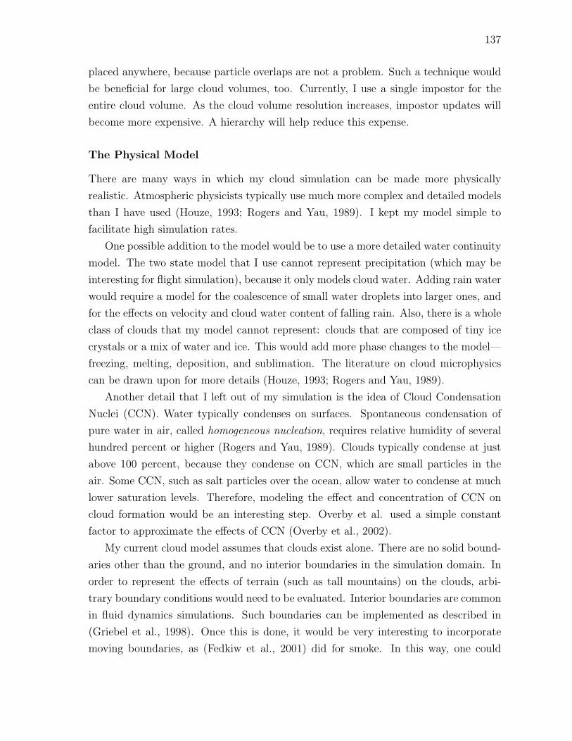
137

placed anywhere, because particle overlaps are not a problem. Such a technique would

be beneficial for large cloud volumes, too. Currently, I use a single impostor for the

entire cloud volume. As the cloud volume resolution increases, impostor updates will

become more expensive. A hierarchy will help reduce this expense.

The Physical Model

There are many ways in which my cloud simulation can be made more physically

realistic. Atmospheric physicists typically use much more complex and detailed models

than I have used (Houze, 1993; Rogers and Yau, 1989). I kept my model simple to

facilitate high simulation rates.

One possible addition to the model would be to use a more detailed water continuity

model. The two state model that I use cannot represent precipitation (which may be

interesting for flight simulation), because it only models cloud water. Adding rain water

would require a model for the coalescence of small water droplets into larger ones, and

for the effects on velocity and cloud water content of falling rain. Also, there is a whole

class of clouds that my model cannot represent: clouds that are composed of tiny ice

crystals or a mix of water and ice. This would add more phase changes to the model—

freezing, melting, deposition, and sublimation. The literature on cloud microphysics

can be drawn upon for more details (Houze, 1993; Rogers and Yau, 1989).

Another detail that I left out of my simulation is the idea of Cloud Condensation

Nuclei (CCN). Water typically condenses on surfaces. Spontaneous condensation of

pure water in air, called homogeneous nucleation, requires relative humidity of several

hundred percent or higher (Rogers and Yau, 1989). Clouds typically condense at just

above 100 percent, because they condense on CCN, which are small particles in the

air. Some CCN, such as salt particles over the ocean, allow water to condense at much

lower saturation levels. Therefore, modeling the effect and concentration of CCN on

cloud formation would be an interesting step. Overby et al. used a simple constant

factor to approximate the effects of CCN (Overby et al., 2002).

My current cloud model assumes that clouds exist alone. There are no solid bound-

aries other than the ground, and no interior boundaries in the simulation domain. In

order to represent the effects of terrain (such as tall mountains) on the clouds, arbi-

trary boundary conditions would need to be evaluated. Interior boundaries are common

in fluid dynamics simulations. Such boundaries can be implemented as described in

(Griebel et al., 1998). Once this is done, it would be very interesting to incorporate

moving boundaries, as (Fedkiw et al., 2001) did for smoke. In this way, one could

138

simulate the effects of aircraft on the clouds, because the moving boundaries of the

aircraft would change the air flow.

Finally, I have not compared the results of a GPU cloud simulation to measured

data from real clouds. Model verification is a common feature of cloud dynamics

research in the atmospheric sciences. Data collected from mountain observatories and

from flight through clouds is available (Rogers and Yau, 1989). This data could be

used for comparison, depending on the level of detail of the simulation. This leads to

another interesting direction—moving beyond visual simulation to accurate numerical

simulation. To do so may require higher precision computation, as I discuss in Section

7.1.3.

Radiometry

Improvements in the radiometry simulation may be beneficial. My multiple forward

scattering approximation produces good results for interactive applications, but as more

computational power becomes available, it may be desirable to spend some of it on a

more realistic scattering model. One existing problem is the expense of computing the

phase function for voxel-based clouds. A method for reducing this cost is needed (see

Section 6.1.6).

My dynamics model does not take into account the effects of radiometry on cloud

dynamics. Sunlight has warming effects on clouds and on the earth below. When clouds

grow thick, they shadow the earth, which cools it, and reduces updrafts. This effects

the air currents, the movement of water vapor, and the formation and motion of clouds.

My illumination model results in a shadow map (for the particle-based algorithm) or

volume (OLV) that could be used to shadow terrain below the clouds, and possibly

determine which areas are warmer than others.

7.1.2 Creative Control

Games are developed by both programmers and artists. Because games often tell stories

and have strong visual themes, artistic control of all features is essential. Therefore,

methods of controlling physically-based cloud simulations (not to mention simulations

of other phenomena) are a useful direction for future work. My simulation provides

simple controls over atmospheric parameters; but these require an understanding of

how clouds form. More intuitive controls—“more whispy”, “more lumpy”—would be

an interesting idea to pursue.

139

My static particle-based clouds provide much more artistic control than my dynamic

clouds simply because they must be constructed by hand (or at least their general shape

must be constructed—see Section 6.1). The nice thing about this is that the artist has

control over each individual cloud. With a dynamic simulation, the control applies to

a field in which clouds—possibly multiple clouds—may form. It would be nice to have

control over the number, shape, and size of clouds that form in a simulated field. The

ability for an artist to say “place a single, dynamic fair-weather cumulus cloud here”

would be very powerful.

7.1.3 GPGPU and Other phenomena

General-purpose computation on GPUs is an area of research that I find very inter-

esting. I think that GPUs will see increasing use in computer games for procedural

texturing and physically-based simulation. Also, the low cost, high speed, and paral-

lelism of GPUs makes them ideal in many ways for scientific computing. Imagine giant

clusters of PCs with powerful GPUs crunching through massive physical and numerical

simulations.

In order to achieve this, some limitations must be removed. For example, current

GPUs support only single-precision (32-bit) floating point numbers. This precision is

currently more than enough for the rendering required by computer games, but many

scientific simulations require double precision. It is unclear whether or not demand for

this precision from the scientific computing community would be enough to convince

GPU manufacturers to support it.

I look forward to seeing many different phenomena simulated on GPUs—possibly

at interactive rates that weren’t achievable before. For example, my cloud simulation

model, with the exception of moving interior boundaries, is a superset of the model

used by (Fedkiw et al., 2001) for smoke simulation. While it may not execute in real

time, GPU simulation is likely faster than simulation on the CPU. More research into

GPU techniques for simulating dynamic phenomena such as fluids is needed.

140

141

Bibliography

Andrews, D. G. (2000). An Introduction to Atmospheric Physics. CambridgeUniversity Press, Cambridge.

ATI Technologies, Inc. (2003). ATI Radeon 9800.http://www.ati.com/products/radeon9800/radeon9800pro/index.html.

Bhate, N. and Tokuta, A. (1992). Photorealistic volume rendering of media withdirectional scattering. In Proceedings of the 3rd Eurographics Workshop onRendering, pages 227–245.

Blasi, P., Le Saec, B., and Schlick, C. (1993). A rendering algorithm for discretevolume density objects. In Proceedings of Eurographics 1993, pages 201–210.

Blinn, J. F. (1982a). A generalization of algebraic surface drawing. In Proceedings ofSIGGRAPH 1982, pages 273–274.

Blinn, J. F. (1982b). Light reflection functions for simulation of clouds and dustysurfaces. In Proceedings of SIGGRAPH 1982, Computer Graphics, pages 21–29.

Bohn, C.-A. (1998). Kohonen feature mapping through graphics hardware. InProceedings of the 3rd Int. Conference on Computational Intelligence andNeurosciences.

Bohren, C. F. (1987). Multiple scattering of light and some of its observableconsequences. American Journal of Physics, 55(6):524–533.

Bolz, J., Farmer, I., Grinspun, E., and Schroder, P. (2003). Sparse matrix solvers onthe GPU: Conjugate gradients and multigrid. In Proceedings of SIGGRAPH2003, pages 917–924.

Briggs, W. L., Henson, V. E., and McCormick, S. F. (2000). A Multigrid Tutorial,Second Edition. SIAM, second edition.

Cabral, B., Cam, N., and Foran, J. (1994). Accelerated volume rendering andtomographic reconstruction using texture mapping hardware. In Proceedings ofthe 1994 Symposium on Volume Visualization, pages 91–98.

Carr, N. A., Hall, J. D., and Hart, J. C. (2002). The ray engine. In Proceedings of theACM SIGGRAPH/EUROGRAPHICS conference on Graphics hardware, pages37–46.

Carr, N. A., Hall, J. D., and Hart, J. C. (2003). GPU algorithms for radiosity andsubsurface scattering. In Proceedings of the ACMSIGGRAPH/EUROGRAPHICS conference on Graphics hardware, pages 51–59.

142

Chandresekhar, S. (1960). Radiative Transfer. Dover, New York.

Chenney, S. and Forsyth, D. (1997). View dependent culling of dynamic systems invirtual environments. In Proceedings of the 1997 symposium on Interactive 3Dgraphics, pages 55–58.

Chorin, A. J. and Marsden, J. E. (1993). A Mathematical Introduction to FluidMechanics, Third Edition. Springer, New York.

Cohen, M. F. and Wallace, J. R. (1993). Radiosity and Realistic Image Synthesis.Morgan Kaufmann.

Coombe, G., Harris, M. J., and Lastra, A. (2003). Radiosity on graphics hardware.Technical Report TR03-020, University of North Carolina.

Cornette, W. and Shanks, J. (1992). Physically reasonable analytic expression for thesingle-scattering phase function. Applied Optics, 31:3152–3160.

Dobashi, Y., Kaneda, K., Yamashita, H., Okita, T., and Nishita, T. (2000). A simple,efficient method for realistic animation of clouds. In Proceedings of SIGGRAPH2000, pages 19–28.

Dobashi, Y., Nishita, T., Yamashita, H., and Okita, T. (1999). Using metaballs tomodeling and animate clouds from satellite images. The Visual Computer,15:471–482.

Eberly, D. H. (2001). 3D Game Engine Design. Morgan Kaufmann Publishers.

Ebert, D. S. (1997). Volumetric modeling with implicit functions: a cloud is born. InACM SIGGRAPH 97 Visual Proceedings: The art and interdisciplinaryprograms of SIGGRAPH ’97, page 245.

Ebert, D. S., Musgrave, F. K., Peachey, D., Perlin, K., and Worley, S. (2002).Texturing & Modeling: A Procedural Approach, Third Edition. MorganKaufman.

Ebert, D. S. and Parent, R. E. (1990). Rendering and animation of gaseousphenomena by combining fast volume and scanline A-buffer techniques. InProceedings of SIGGRAPH 1990, pages 357–366.

Elinas, P. and Sturzlinger, W. (2001). Real-time rendering of 3D clouds. The Journalof Graphics Tools, 5(4):33–45.

England, J. N. (1978). A system for interactive modeling of physical curved surfaceobjects. In Proceedings of SIGGRAPH 1978, pages 336–340.

Eyles, J., Molnar, S., Poulton, J., Greer, T., and Lastra, A. (1997). Pixelflow: Therealization. In Proceedings of the ACM SIGGRAPH/EUROGRAPHICSworkshop on Graphics hardware, pages 57–68.

143

Fedkiw, R., Stam, J., and Jensen, H. W. (2001). Visual simulation of smoke. InProceedings of SIGGRAPH 2001, pages 15–22.

Fernando, R., editor (2004). GPU Gems: Programming Techniques, Tips and Tricksfor Real-Time Graphics. Addison Wesley Professional.

FlightGear (2003). FlightGear Flight Simulator. http://www.flightgear.org/.

Foster, N. and Metaxas, D. (1997). Modeling the motion of a hot, turbulent gas. InProceedings of SIGGRAPH 1997, pages 181–188.

Gardner, G. Y. (1985). Visual simulation of clouds. In Proceedings of SIGGRAPH1985, pages 297–303.

Golub, G. H. and Van Loan, C. F. (1996). Matrix Computations, Third Edition. TheJohns Hopkins University Press, Baltimore.

Goodnight, N., Woolley, C., Lewin, G., Luebke, D., and Humphreys, G. (2003). Amultigrid solver for boundary value problems using graphics hardware. InProceedings of the ACM SIGGRAPH/EUROGRAPHICS conference onGraphics hardware, pages 102–111.

Govindaraju, N., Redon, S., Lin, M. C., and Manocha, D. (2003). Cullide: Interactivecollision detection between complex models in large environments using graphicshardware. In Proceedings of the ACM SIGGRAPH/EUROGRAPHICSconference on Graphics hardware, pages 25–32.

Griebel, M., Dornseifer, T., and Neunhoeffer, T. (1998). Numerical Simulation inFluid Dynamics : A Practical Introduction. SIAM Monographs onMathematical Modeling and Computation. Society for Industrial and AppliedMathematics, Philadelphia.

Guha, S., Krishnan, S., Munagala, K., and Venkatasubramanian, S. (2003).Application of the two-sided depth test to CSG rendering. In Proceedings of the2003 symposium on Interactive 3D graphics, pages 177–180.

Hamblyn, R. (2001). The Invention of Clouds. Picador USA.

Harris, M. J. (2002a). Analysis of error in a CML diffusion operation. TechnicalReport TR02-015, University of North Carolina.

Harris, M. J. (2002b). Implementation of a CML boiling simulation using graphicshardware. Technical Report TR02-016, University of North Carolina.

Harris, M. J., Baxter, W. V., Scheuermann, T., and Lastra, A. (2003). Simulation ofcloud dynamics on graphics hardware. In Proceedings of the ACMSIGGRAPH/EUROGRAPHICS conference on Graphics hardware, pages92–101.

144

Harris, M. J., Coombe, G., Scheuermann, T., and Lastra, A. (2002). Physically-basedvisual simulation on graphics hardware. In Proceedings of the ACMSIGGRAPH/EUROGRAPHICS conference on Graphics hardware, pages109–118.

Harris, M. J. and James, G. (2003). Simulation and animation using hardwareaccelerated procedural textures. In Proceedings of Game Developers Conference2003.

Harris, M. J. and Lastra, A. (2001). Real-time cloud rendering. In Proceedings ofEurographics 2001, pages 76–84.

Heidrich, W., Westermann, R., Seidel, H.-P., and Ertl, T. (1999). Applications ofpixel textures in visualization and realistic image synthesis. In Proceedings ofthe 1999 symposium on Interactive 3D graphics, pages 127–134.

Henyey, L. and Greenstein, J. (1941). Diffuse radiation in the galaxy. TheAstrophysical Journal, 90:70–83.

Hillesland, K., Molinov, S., and Grzeszczuk, R. (2003). Nonlinear optimizationframework for image-based modeling on programmable graphics hardware. InProceedings of SIGGRAPH 2003, pages 925–934.

Hoff, K. E., Culver, T., Keyser, J., Lin, M., and Manocha, D. (1999). Fastcomputation of generalized voronoi diagrams using graphics hardware. InProceedings of SIGGRAPH 1999, pages 277–286.

Hoff, K. E., Zaferakis, A., Lin, M., and Manocha, D. (2001). Fast and simple 2Dgeometric proximity queries using graphics hardware. In Proceedings of the 2001Symposium on Interactive 3D Graphics, pages 145–148.

Houze, R. (1993). Cloud Dynamics. International Geophysics Series. Academic Press,San Diego.

Howard, L. (1804). On the Modifications of Clouds. J. Taylor, London.

iROCK Games (2002). Savage Skies. Bam! Entertainment.

James, G. (2001a). NVIDIA Game Of Life Demo.http://developer.nvidia.com/view.asp?IO=ogl gameoflife.

James, G. (2001b). NVIDIA Procedural Texture Physics Demo.http://developer.nvidia.com/view.asp?IO=ogl dynamic bumpreflection.

James, G. (2001c). Operations for hardware-accelerated procedural textureanimation. In Deloura, M., editor, Game Programming Gems 2, pages 497–509.Charles River Media.

145

Jensen, H. W. (1996). Global illumination using photon maps. In Proceedings of the7th Eurographics Workshop on Rendering, pages 21–30.

Jensen, H. W. and Christensen, P. H. (1998). Efficient simulation of light transport inscences with participating media using photon maps. In Proceedings ofSIGGRAPH 1998, pages 311–320.

Jobard, B., Erlebacher, G., and Hussaini, M. Y. (2001). Lagrangian-eulerian advectionfor unsteady flow visualization. In Proceedings of IEEE Visualization 2001.

Kajiya, J. T. and Von Herzen, B. P. (1984). Ray tracing volume densities. InProceedings of SIGGRAPH 1984, pages 165–174.

Kaneko, K., editor (1993). Theory and applications of coupled map lattices. NonlinearScience: theory and applications. Wiley.

Kapral, R. (1993). Chemical waves and coupled map lattices. In Kaneko, K., editor,Theory and Applications of Coupled Map Lattices, pages 135–168. Wiley.

Kedem, G. and Ishihara, Y. (1999). Brute force attack on UNIX passwords withSIMD computer. In Proceedings of The 8th USENIX Security Symposium.

Kim, T. and Lin, M. C. (2003). Visual simulation of ice crystal growth. InProceedings of the 2003 ACM SIGGRAPH/Eurographics Symposium onComputer Animation, pages 86–97.

Klassen, R. V. (1987). Modeling the effect of the atmosphere on light. ACMTransactions on Graphics, 6(3):215–237.

Kniss, J., Premoze, S., Hansen, C., and Ebert, D. S. (2002). Interactive translucentvolume rendering and procedural modeling. In Proceedings of IEEEVisualization 2002, pages 109–116.

Krishnan, S., Mustafa, N. H., and Venkatasubramanian, S. (2002). Hardware-assistedcomputation of depth contours. In Proceedings of the thirteenth annualACM-SIAM symposium on Discrete algorithms.

Kruger, J. and Westermann, R. (2003). Linear algebra operators for GPUimplementation of numerical algorithms. In Proceedings of SIGGRAPH 2003.

Lacroute, P. and Levoy, M. (1994). Fast volume rendering using a shear-warpfactorization of the viewing transformation. In Proceedings of SIGGRAPH 1994,pages 451–458.

Larsen, E. S. and McAllister, D. K. (2001). Fast matrix multiplies using graphicshardware. In Proceedings of the 2001 ACM/IEEE conference on Supercomputing(CDROM).

146

Laven, P. (2003). MiePlot Software. http://philiplaven.com/MiePlot.htm.

Lee, K. J., McCormick, W. D., Ouyang, Q., and Swinn, H. L. (1993). Patternformation by interacting chemical fronts. Science, 261:192–194.

Lefohn, A. E., Kniss, J., Hansen, C., and Whitaker, R. T. (2003). Interactivedeformation and visualization of level set surfaces using graphics hardware. InProceedings of IEEE Visualization 2003.

Lefohn, A. E. and Whitaker, R. T. (2002). A GPU-based, three-dimensional level setsolver with curvature flow. Technical Report UUCS-02-017, University of Utah.

Lengyel, J., Reichert, M., Donald, B. R., and Greenberg, D. P. (1990). Real-timerobot motion planning using rasterizing computer graphics hardware. InProceedings of SIGGRAPH 1990, pages 327–335.

Levoy, M. (1988). Display of surfaces from volume data. IEEE Computer Graphics &Applications, 8(3):29–37.

Lewis, J. P. (1989). Algorithms for solid noise synthesis. In Proceedings ofSIGGRAPH 1989, pages 263–270.

Li, W., Wei, X., and Kaufman, A. (2003). Implementing lattice boltzmanncomputation on graphics hardware. Technical Report 010416, State Universityof New York at Stony Brook.

Lindholm, E., Kilgard, M., and Moreton, H. (2001). A user programmable vertexengine. In Proceedings of SIGGRAPH 2001, pages 149–158.

Maciel, P. W. C. and Shirley, P. (1995). Visual navigation of large environments usingtextured clusters. In Proceedings of the 1995 symposium on Interactive 3Dgraphics, pages 95–ff.

Mark, W. R., Glanville, R. S., Akeley, K., and Kilgard, M. J. Cg: A system forprogramming graphics hardware in a C-like language. In Proceedings ofSIGGRAPH 2003, pages 896–907.

Max, N. (1994). Efficient light propagation for multiple anisotropic volume scattering.In Proceedings of the 5th Eurographics Workshop on Rendering, pages 87–104.

Max, N. (1995). Optical models for direct volume rendering. IEEE Transactions onVisualization and Computer Graphics, 1(2):99–108.

Microsoft (2003). DirectX API. http://www.microsoft.com/directx.

Mie, G. (1908). Bietage zur optik truver medien speziell kolloidaler metallosungen.Annallen der Physik, 25(3):377.

147

Miyazaki, R., Yoshida, S., Dobashi, Y., and Nishita, T. (2001). A method formodeling clouds based on atmospheric fluid dynamics. In Proceedings of PacificGraphics 2001, pages 363–372.

Mustafa, N. H., Koutsofios, E., Krishnan, S., and Venkatasubramanian, S. (2001).Hardware assisted view dependent map simplification. In Proceedings of the17th Annual Symposium on Computational Geometry.

Nagel, K. and Raschke, E. (1992). Self-organizing criticality in cloud formation?Physica A, 182:519–531.

Neyret, F. (1997). Qualitative simulation of cloud formation and evolution. InProceedings of the 8th Eurographics Workshop on Computer Animation andSimulation, pages 113–124.

Neyret, F. (2003). Advected textures. In Proceedings of the 2003 ACMSIGGRAPH/Eurographics Symposium on Computer Animation, pages 147–153.

Nishimori, H. and Ouchi, N. (1993). Formation of ripple patterns and dunes bywind-blown sand. Physical Review Letters, 71(1):197–200.

Nishita, T., Dobashi, Y., and Nakamae, E. (1996). Display of clouds taking intoaccount multiple anisotropic scattering and sky light. In Proceedings ofSIGGRAPH 1996, pages 379–386.

NVIDIA Corporation (2001). GeForce 3. http://www.nvidia.com/page/geforce3.html.

NVIDIA Corporation (2002a). GeForce 4 Ti.http://www.nvidia.com/page/geforce4ti.html.

NVIDIA Corporation (2002b). NVIDIA OpenGL Extension Specifications.http://developer.nvidia.com/view.asp?IO=nvidia opengl specs.

NVIDIA Corporation (2003). GeForce FX.http://www.nvidia.com/page/fx desktop.html.

Olano, M. and Lastra, A. (1998). A shading language on graphics hardware: Thepixelflow shading system. In Proceedings of SIGGRAPH 1998, pages 159–168.

Overby, D., Melek, Z., and Keyser, J. (2002). Interactive physically-based cloudsimulation. In Proceedings of Pacific Graphics 2002, pages 469–470.

Patmore, C. (1993). Simulated multiple scattering for cloud rendering. In Graphics,Design and Visualization, Proceedings of the IFIP TC5/WG5.2/WG5.10 CSIInternational Conference on Computer Graphics, pages 29–40.

Pearson, J. E. (1993). Complex patterns in a simple system. Science, 261:189–192.

148

Peercy, M. S., Olano, M., Airey, J., and Ungar, P. J. (2000). Interactive multi-passprogrammable shading. In Proceedings of SIGGRAPH 2000, pages 425–432.

Perlin, K. (1985). An image synthesizer. In Proceedings of SIGGRAPH 1985, pages287–296.

Perlin, K. and Neyret, F. (2001). Flow noise. In SIGGRAPH 2001 Technical Sketchesand Applications, page 187.

Poddar, B. and Womack, P. (2001). WGL ARB render texture OpenGL extensionspecification.http://oss.sgi.com/projects/ogl-sample/registry/ARB/wgl render texture.txt.

Potmesil, M. and Hoffert, E. M. (1989). The pixel machine: A parallel imagecomputer. In Proceedings of SIGGRAPH 1989, pages 69–78.

Premoze, S., Harris, M. J., Hoffman, N., and Preetham, A. J. (2003). Light and colorin the outdoors. In SIGGRAPH 2003 Course Notes (#1).

Proudfoot, K., Mark, W. R., Tzvetkov, S., and Hanrahan, P. (2001). A real-timeprocedural shading system for programmable graphics hardware. In Proceedingsof SIGGRAPH 2001, pages 159–170.

Purcell, T. J., Buck, I., Mark, W. R., and Hanrahan, P. (2002). Ray tracing onprogrammable graphics hardware. In Proceedings of SIGGRAPH 2002, pages703–712.

Purcell, T. J., Donner, C., Cammarano, M., Jensen, H. W., and Hanrahan, P. (2003).Photon mapping on programmable graphics hardware. In Proceedings of theACM SIGGRAPH/EUROGRAPHICS conference on Graphics hardware, pages41–50.

Qian, Y., Succi, S., and Orszag, S. (1996). Recent advances in lattice boltzmanncomputing. In Stauffer, D., editor, Annual Reviews of Computational PhysicsIII, pages 195–242. World Scientific.

Reeves, W. (1983). Particle systems—a technique for modeling a class of fuzzyobjects. In Proceedings of SIGGRAPH 1983, pages 359–375.

Reeves, W. and Blau, R. (1985). Approximate and probabilistic algorithms forshading and rendering structured particle systems. In Proceedings ofSIGGRAPH 1985, pages 313–322.

Rhoades, J., Turk, G., Bell, A., State, A., Neumann, U., and Varshney, A. (1992).Real-time procedural textures. In Proceedings of the 1992 Symposium onInteractive 3D Graphics, pages 95–100.

149

Rogers, R. R. and Yau, M. K. (1989). A Short Course in Cloud Physics, ThirdEdition. International Series in Natural Philosophy. Butterworth Heinemann,Burlington, MA.

Rushmeier, H. E. and Torrance, K. E. (1987). The zonal method for calculating lightintensities in the presence of a participating medium. In Proceedings ofSIGGRAPH 1987, pages 293–302.

Schaufler, G. (1995). Dynamically generated impostors. In Proceedings of the GIWorkshop “Modeling—Virtual Worlds—Distributed Graphics”, pages 129–135.

Schpok, J., Simons, J., Ebert, D. S., and Hansen, C. (2003). A real-time cloudmodeling, rendering, and animation system. In Proceedings of the 2003 ACMSIGGRAPH/Eurographics Symposium on Computer Animation, pages 160–166.

Segal, M. and Akeley, K. (2001). The OpenGL Graphics System: A Specification(Version 1.3). http://www.opengl.org.

Shade, J., Lischinski, D., Salesin, D. H., DeRose, T., and Snyder, J. (1996).Hierarchical image caching for accelerated walkthroughs of complexenvironments. In Proceedings of SIGGRAPH 1996, pages 75–82.

Srivastava, R. (1967). A study of the effect of precipitation on cumulus dynamics.Journal of Atmospheric Science, 24:36–45.

Stam, J. (1995). Multiple scattering as a diffusion process. In Proceedings of the 6thEurographics Workshop on Rendering, pages 41–50.

Stam, J. (1999). Stable fluids. In Proceedings of SIGGRAPH 1999, pages 121–128.

Stam, J. (2003). Real-time fluid dynamics for games. In Proceedings of the GameDevelopers Conference.

Steiner, J. (1973). A three-dimensional model of cumulus cloud development. Journalof Atmospheric Science, 30:414–435.

Stewart, N., Leach, G., and John, S. (2003). Improved CSG rendering using overlapgraph subtraction sequences. In Proceedings of the International Conference onComputer Graphics and Interactive Techniques in Australasia and South EastAsia (GRAPHITE 2003), pages 47–53.

Strutt, J. W. (1871). On the light from the sky, its polarization and colour. Philos.Mag., 41:107–120, 274–279.

Strzodka, R. (2002). Virtual 16 bit precise operations on RGBA8 textures. InProceedings of Vision, Modeling, and Visualization.

150

Strzodka, R. and Rumpf, M. (2001). Level set segmentation in graphics hardware. InProceedings of the International Conference on Image Processing.

Takeda, T. (1971). Numerical simulation of a precipitating convective cloud: theformation of a “long-lasting” cloud. Journal of Atmospheric Science,28:350–376.

Thompson, C. J., Hahn, S., and Oskin, M. (2002). Using modern graphicsarchitectures for general-purpose computing: A framework and analysis. InProceedings of the International Symposium on Microarchitecture (IEEEMICRO), pages 306–320.

Toffoli, T. and Margolus, N. (1987). Cellular Automata Machines. The MIT Press,Cambridge, Massachusetts.

Trendall, C. and Steward, A. J. (2000). General calculations using graphics hardware,with applications to interactive caustics. In Proceedings of the EurographicsWorkshop on Rendering, pages 287–298.

Turing, A. M. (1952). The chemical basis of morphogenesis. Transactions of theRoyal Society of London, (B237):37–72.

Turk, G. (1991). Generating textures on arbitrary surfaces using reaction-diffusion. InProceedings of SIGGRAPH 1991, pages 289–298.

van de Hulst, H. (1981). Light Scattering by Small Particles. Dover.

Veach, E. (1997). Robust Monte Carlo Methods for Light Transport Simulation. Ph.d.dissertation, Stanford University.

von Neumann, J. (1966). Theory of Self-Reproducing Automata. University of IllinoisPress. Edited and completed by A.W. Burks.

Weiskopf, D., Hopf, M., and Ertl, T. (2001). Hardware-accelerated visualization oftime-varying 2D and 3D vector fields by texture advection via programmableper-pixel operations. In Proceedings of Vision, Modeling, and Visualization,pages 439–446.

Weisstein, E. W. (1999). CRC Concise Encyclopedia of Mathematics. CRC Press.

Westover, L. (1990). Footprint evaluation for volume rendering. In Proceedings ofSIGGRAPH 1990, pages 367–376.

Wilson, O., Van Gelder, A., and Wilhelms, J. (1994). Direct volume rendering via 3Dtextures. Technical Report UCSC-CRL-94-19, University of California at SantaCruz.

151

Witkin, A. and Kass, M. (1991). Reaction-diffusion textures. In Proceedings ofSIGGRAPH 1991, pages 299–308.

Wojnaroski, J. (2003). Personal communication.

Wolfram, S. (1984). Cellular automata as models of complexity. Nature,(311):419–424.

Yanagita, T. (1992). Phenomenology of boiling: A coupled map lattice model. Chaos,2(3):343–350.

Yanagita, T. and Kaneko, K. (1993). Coupled map lattice model for convection.Physics Letters A, 175:415–420.

Yanagita, T. and Kaneko, K. (1997). Modeling and characterization of clouddynamics. Physical Review Letters, 78(22):4297–4300.

Yang, R., Welch, G., and Bishop, G. (2002). Real-time consensus-based scenereconstruction using commodity graphics hardware. In Proceedings of PacificGraphics 2002.