Real Options, Volatility, and Stock Returns

GUSTAVO GRULLON, EVGENY LYANDRES, and ALEXEI ZHDANOV∗

ABSTRACT

We provide evidence that the positive relation between firm-level

stock returns and firm-level return volatility is due to firms’ real options.

Consistent with real option theory, we find that the positive volatility-

return relation is much stronger for firms with more real options and

that the sensitivity of firm value to changes in volatility declines signifi-

cantly after firms exercise their real options. We reconcile the evidence

at the aggregate and firm levels by showing that the negative relation

at the aggregate level may be due to aggregate market conditions that

simultaneously affect both market returns and return volatility.

∗Gustavo Grullon is with the Jesse H. Jones Graduate School of Business, Rice Univeristy.Evgeny Lyandres is with the School of Management, Boston University. Alexei Zhdanov is with theUniversity of Lausanne and Swiss Finance Institute. The authors thank Rui Abuquerque, YakovAmihud, Doron Avramov, Clifford Ball, Alexander Barinov, Jonathan Berk, Gennaro Bernile,Nicolas Bollen, Jacob Boudoukh, Tim Burch, Murray Carlson, Lauren Cohen, Francois Degeorge,Darrell Duffie, Rafi Eldor, Wayne Ferson, Amit Goyal, Dirk Hackbarth, Campbell Harvey (the Ed-itor), Ohad Kadan, Markku Kaustia, Matti Keloharju, Timo Korkeamaki, Moshe Levy, LubomirLitov, Hong Liu, Roni Michaely, Barb Ostdiek, Dino Palazzo, Brad Paye, Neil Pearson, GordonPhillips, Lukasz Pomorski, Amir Rubin, Jacob Sagi, Dan Segal, Anjan Thakor, Yuri Tserlukevich,Masahiro Watanabe, James Weston, Zvi Wiener, Yuhang Xing, Guofu Zhou, an associate editor,an anonymous referee, and seminar participants at Aalto School of Economics, Hebrew Univer-sity, Interdisciplinary Center Herzliya, Louisiana State University, Rice University, Texas A&MInternational University, Vanderbilt University, Washington University at Saint Louis, Universityof Illinois at Urbana-Champaign, University of Miami, University of Texas at San Antonio, 2008University of British Columbia Winter Finance Conference, 2008 Rotschild Caesarea Center Con-ference, 2008 European Finance Association Meetings, 2011 Finance Down Under Conference, and2011 Napa Valley Conference for helpful comments and suggestions. The authors also thank Her-nan Ortiz-Molina for help with using union membership data and Sarah Diez for valuable researchassistance.

It is well established in the asset pricing literature that aggregate market returns are

negatively correlated with aggregate market volatility (e.g., French, Schwert, and

Stambaugh (1987), Campbell and Hentschel (1992), and Duffee (1995)). One pos-

sible explanation for this negative relation is the “leverage effect” hypothesis (e.g.,

Black (1976) and Christie (1982)), which states that when stock prices fall, firms

become more levered, raising the volatility of stock returns. Another explanation,

due to French, Schwert, and Stambaugh (1987), holds that because an increase in

systematic volatility raises risk premia and expected future stock returns, an unex-

pected change in (systematic) volatility is likely to reduce firm values, leading to a

negative association between volatility and contemporaneous returns.

Contrary to the evidence at the aggregate level, however, Duffee (1995) finds

that stock returns and volatility are positively correlated at the firm level. This

empirical finding has important theoretical implications because it is inconsistent

with the leverage and risk premia hypotheses, and it challenges the conventional

wisdom on the relation between volatility and asset prices.

The main contribution of our paper is twofold. First, we provide a rational

explanation for the positive contemporaneous relation between firm-level returns and

firm-level volatility documented in Duffee (1995). Second, we provide an explanation

for the difference between the aggregate volatility-return relation and the firm-level

volatility-return relation. Surprisingly, despite the importance of these issues to our

understanding of the role of volatility in asset pricing, research on these topics has

been very limited (e.g., Albuquerque (2012) and Duffee (2002)).

We hypothesize that the positive relation between firm-level returns and firm-

level volatility may be due to real options that firms possess. One of the main

implications of real options theory is that a real option’s value is increasing in the

1

volatility of an underlying process (i.e., demand volatility, cost volatility, or overall

volatility of profits). The main rationale for this relation is that since firms can

change their operating and investment decisions to mitigate the effects of bad news

(e.g., reduce production, shut down operations, defer investments) and amplify the

effects of good news (e.g., expand production, restart operations, expedite invest-

ments), an increase in the volatility of an underlying process can have a positive

effect on firm value. That is, since operating and investment flexibility increases the

convexity of firm value with respect to the value of its underlying assets, firm value

is an increasing function of volatility, due to Jensen’s inequality. Therefore, if real

options constitute a substantial component of firm value, then it is possible that

the positive return-volatility relation documented in Duffee (1995) is driven by the

presence of these options. We test this hypothesis empirically and find numerous

pieces of supportive evidence.

First, we examine whether the value of firms with abundant investment op-

portunities is more sensitive to changes in underlying volatility than the value of

assets-in-place-based firms. The more investment opportunities a firm has, the more

discretion it has with respect to the timing of its investments and hence the larger

the value of its real options. Thus, if the positive relation between returns and

changes in volatility is due to the presence of real options, whose values are increas-

ing in volatility, then the sensitivity of firm value to volatility should be stronger

among firms with more investment opportunities. Using a battery of proxies for in-

vestment opportunities, we find that the positive contemporaneous relation between

returns and changes in volatility is very strong among firms that are likely to have

abundant investment opportunities, while it is substantially weaker among assets in

place-based firms. Specifically, we find that the volatility-return relation is stronger

2

among young firms, small firms, high R&D firms, and high growth firms.

Second, since the value of real options comes from the ability of firm managers to

change their decisions as new information arrives, we also investigate whether proxies

for operating flexibility can explain cross-sectional differences in the volatility-return

relation. Consistent with the prediction that volatility creates value when managers

have flexibility to alter their investment and operating decisions, we find that the

relation between volatility and stock returns is stronger among firms with fewer op-

erational constraints (e.g., firms in non-unionized industries) and firms that appear

to be able to respond better to resolutions of uncertainty (e.g., firms with higher

convexity of value with respect to earnings and sales).

Third, we investigate how the sensitivity of firm values to changes in volatility

evolves as a firm’s mix of growth options and assets in place changes over time. On

the one hand, a firm develops and accumulates real options. On the other hand, it

exercises these options by investing when the value of the benefits from investing

is high enough to offset the value of the option to wait. Thus, the sensitivity of

firm value to changes in volatility is expected to be increasing as the firm builds

up its real options, and it is expected to decline when the firm exercises (part of)

them. To test this prediction, we use spikes in firms’ investment levels, issues of

seasoned equity, and spikes in external financing in general to proxy for instances

of real option exercises. Consistent with the theory, we find that the sensitivity of

firm value to changes in underlying volatility increases prior to real option exercises,

drops sharply following exercises of real options, and then starts rising again as firms

start to build up new real options. This evidence strongly suggests that part of the

positive relation between returns and volatility is driven by the effect of volatility

on the value of real options.

3

Fourth, we demonstrate that the volatility-return relation is much stronger in

industries that have been shown to have plenty of growth and strategic options (high-

tech, pharmaceutical, and biotechnology industries) and high levels of operating

flexibility (natural resources industry). Furthermore, we perform a within-industry

analysis using a sample of oil and gas firms to investigate more deeply the effect

of volatility on stock returns. We focus on oil and gas firms because they provide

a unique setting for testing the predictions of the real options theory. Since these

firms have valuable timing options on developing their undeveloped proven reserves,

one could use their undeveloped and developed reserve estimates as proxies for their

mix of real options and assets in place. Using hand-collected data on oil and gas

firms’ reserves, we find that, consistent with the theory, the return-volatility relation

is stronger among firms with a higher proportion of undeveloped reserves.

In addition, we examine the effect of the return-volatility relation on the per-

formance of asset pricing models. Based on the insights of McDonald and Siegel

(1985) and Berk, Green, and Naik (1999), Da, Guo, and Jagannathan (2012) argue

that in the presence of real options, the CAPM may explain the expected returns

on a firm’s underlying assets but not necessarily the expected returns on its equity.

This is because when firms possess real options, equity risk becomes a nonlinear

function of the risk of the underlying assets. Consistent with this argument, Da,

Guo, and Jagannathan (2012) show that the presence of real options seems to ex-

plain the poor performance of the CAPM. We exploit this result to test our main

hypothesis. If real options are an important determinant of the positive relation

between volatility and stock returns, then the CAPM, or any asset pricing model

that does not account for real options, should perform better for firms with a weak

return-volatility relation (firms with relatively few real options) than for firms with

4

a strong return-volatility relation (firms with abundant real options). Our empir-

ical results are consistent with the real options theory. Using Gibbons, Ross, and

Shanken’s (1989) test, we find that the CAPM, as well as Fama and French (1993)

three-factor model, cannot be rejected within a subsample of firms with a relatively

weak return-volatility relation, but the models are comfortably rejected within a

subsample of firms with a relatively strong return-volatility relation.

In general, we believe that our paper provides an explanation for the positive

contemporaneous relation between firm-level returns and firm-level volatility docu-

mented in Duffee (1995). The sensitivity of the value of real options to underlying

volatility seems to be an important reason for the cross-sectional variation in the

relation between returns and contemporaneous changes in volatility and for the

evolution of this relation around investment and financing spikes. These findings

complement the existing literature examining the effects of real options on asset

prices (e.g., Berk, Green, and Naik (1999) and Carlson, Fisher, and Giammarino

(2004)).

While the real options hypothesis is consistent with the positive relation be-

tween volatility and stock returns at the firm level, it cannot explain the negative

correlation between these variables at the aggregate level. We argue that the nega-

tive relation between aggregate stock returns and aggregate return volatility could

be driven by an omitted variable problem. Because investors tend to be more un-

certain about future real output growth during economic downturns (e.g., Veronesi

(1999)), periods of high stock return volatility could coincide with periods of low

stock returns even if the direct effect of volatility on firm value is positive. That

is, volatility may increase when stock prices decline not because the fundamental

relation between these variables is negative, but because both variables are affected

5

by the same underlying macroeconomic factors. Thus, regressing aggregate stock

returns on aggregate market volatility could lead to inferences that are very dif-

ferent from those obtained in a setting in which aggregate (market) conditions are

controlled for.

We address this issue by focusing on firm-level stock returns rather than on

aggregate returns. Using individual stock returns instead of aggregate returns allows

us to control simultaneously for aggregate factors (proxies for market conditions)

and aggregate volatility. Consistent with the aggregate evidence, regressions of firm-

level returns on aggregate volatility alone reveal a strong negative return-volatility

relation. However, once we control for aggregate market factors (aggregate market

returns, HML, and SMB), aggregate volatility becomes unrelated to stock returns.

More interestingly, we find that aggregate volatility has a positive effect on the

value of real options-based firms and a negative effect on the value of assets in

place-based firms after controlling for market conditions. These results seem to

reconcile the aggregate-level negative relation between volatility and returns with

the positive relation at the firm level.

The remainder of the paper is organized as follows. In Section I we discuss and

motivate our measure of volatility, summarize the data, and present selected sum-

mary statistics. In Section II we estimate the relation between returns and changes

in volatility for subsets of firms characterized by different mixes of real options and

assets in place. Section III investigates the effect of operating flexibility on the

volatility-return relation. Section IV examines the evolution of the relation between

returns and changes in volatility around times of significant changes in firms’ mix of

real options and assets in place. In Section V we perform an industry-level analysis

of the relation between returns and contemporaneous changes in volatility. In Sec-

6

tion VI we examine the effect of the volatility-return relation on the performance

of asset pricing models. Section VII provides evidence that aggregate volatility is

unrelated to stock returns after controlling for underlying market conditions and

examines the relation between returns and aggregate volatility for subsamples of

real options-based and assets in place-based firms. In Section VIII we discuss the

results of robustness checks. Section IX summarizes and concludes.

I. Measure of Volatility, Data Sources, and Summary

Statistics

A. Measure of Volatility

Theoretically, the value of a firm’s real options is increasing in the volatility of

an underlying process (e.g., McDonald and Siegel (1986)). However, many aspects

of uncertainty regarding potential projects, which include but are not limited to

demand shocks (changes in consumer tastes), supply shocks (changes in production

technologies), and institutional changes, are unobservable. Moreover, even if the

realizations of these shocks were observable ex-post, their expectations, which affect

the value of real options, would not be known. If stock prices incorporate the value

of real options, then the volatility of stock prices is expected to be related to the

volatility of the underlying valuation processes. This justifies the use of measures

stock return volatility as proxies for underlying volatility, as in Leahy and Whited

(1996) and Bulan (2005).

We follow Ang et al. (2006, 2009) and Duffee (1995), among others, and estimate

firm i’s volatility during month t as the standard deviation of the firm’s daily returns

7

during month t,

V OLi,t =

√√√√∑τ∈t

(ri,τ − ri,t)2

nt − 1, (1)

where ri,τ is the natural logarithm of day τ ∈ t gross excess return on firm i’s

stock, ri,t is the mean of the logarithms of gross daily returns on firm i’s stock

during month t, and nt is the number of nonmissing return observations during

month t. We use logarithmic returns to mitigate the potential mechanical effect of

return skewness (see Duffee (1995) and Kapadia (2007)) on the relation between

returns and contemporaneous return volatilities. The change in volatility in month

t, ∆V OLi,t, is computed as the difference between the estimated volatility in month

t and the estimated volatility in month t− 1:

∆V OLi,t = V OLi,t − V OLi,t−1. (2)

B. Main Data Sources and Summary Statistics

We obtain daily stock returns, used in estimating volatilities and factor load-

ings, and monthly returns, used as the dependent variable in our regressions, from

CRSP daily and monthly return files, respectively. Daily and monthly factor returns

and risk-free rates are from Ken French’ website (http:// mba.tuck.dartmouth.edu/

pages/faculty/ken.french/data library.html). The time frame of our analysis is from

January 1964 to December 2008. Following Ang et al. (2006), among others, we

eliminate utilities (SIC codes between 4900 and 4999) and financials (SIC codes be-

tween 6000 and 6999) from the sample. Our sample contains over 3 million monthly

observations with nonmissing returns and volatility estimates.

Accounting variables used to compute firm characteristics, measures of invest-

ment opportunities (firm size, R&D expenditures, and sales growth), measures of op-

erating flexibility (sensitivity of firm value to profits and sales), as well as measures of

8

investment and financing spikes, are from COMPUSTAT. We obtain firms’ founding

and incorporation years, used to compute firm age, from Boyan Jovanovic’s website

(www.nyu.edu/econ/user/jovanovi). Dates of firms’ earnings announcements used

to estimate some of the measures of operating flexibility are from I/B/E/S. Data on

membership in labor unions are obtained from the Union Membership and Cover-

age database (www.unionstats.com), described by Hirsch and Macpherson (2003).1

We obtain data on seasoned equity offerings (SEOs), used in our event-time tests,

from Thomson Financial’s Securities Data Company. Finally, for our analysis of the

effects of real options on the return-volatility relation in the oil and gas industry,

we hand-collect data on developed and total proven oil and gas reserves for 72 oil

firms between 1995 and 2009 from firms’ annual reports.

We present summary statistics for returns, return volatilities, and changes in

return volatility in Table I, which also includes summary statistics for measures of

investment opportunities and managerial flexibility, which we discuss below. The Insert Ta-

ble I heremean excess return in our sample is 0.6% per month or about 7.2% per year. The

mean (median) daily firm-level stock return standard deviation is 3.17% (2.45%).

Our firm-level volatility estimates using daily data are similar to those reported

in Ang et al. (2006). The small positive mean change in volatility (0.007%) is

consistent with the positive time trend in volatility (e.g., Campbell et al. (2001)

and Cao, Simin, and Zhao (2008)). The standard deviation of the month-to-month

change in return volatility is 1.83%.

II. Return-Volatility Relation and Investment

Opportunities

We begin by verifying that the positive relation between firm-level volatility and

9

firm-level returns documented in Duffee (1995, 2002) and Albuquerque (2012) holds

in our sample. In particular, we estimate monthly cross-sectional Fama-MacBeth

(1973) regressions of individual firm returns, ri,t, net of the risk-free rate, rf,t, on

contemporaneous changes in firm-level volatility, ∆V OLi,t, and a vector of firm

characteristics, xi,t, most of which are known at the beginning of month t:

ri,t − rf,t = αt + βt∆V OLi,t + γt ηMKTi,t +−→δtxi,t + εi,t. (3)

Following common practice in the asset pricing literature (e.g., Fama and French

(1993), Jegadeesh and Titman (1993), and Cooper, Gulen, and Schill (2008) among

many others), these characteristics are log market equity, log book-to-market, and

past returns. Following Fama and French (1993), we measure the market value of

equity as the share price at the end of June times the number of shares outstanding.

Book equity is stockholders’ equity minus preferred stock plus balance sheet deferred

taxes and investment tax credit if available, minus post-retirement benefit assets if

available. If stockholders’ equity is missing, we use common equity plus preferred

stock par value. If these variables are missing, we use book assets less liabilities.

Preferred stock is preferred stock liquidating value, preferred stock redemption value,

or preferred stock par value in that order of availability. To compute the book-

to-market ratio, we use the December closing stock price times number of shares

outstanding. We match returns from January to June of year t with COMPUSTAT-

based variables of year t−2, while the returns from July until December are matched

with COMPUSTAT variables of year t−1. Past returns are defined as buy-and-hold

returns for six months over months [t−7, t−2]. In addition, following Karpoff (1987),

we include contemporaneous trading volume, normalized by the number of shares

outstanding. The estimated coefficient on the market portfolio return, ηMKTi,t in

10

(3), is obtained from the following regression:

ri,τ − rf,τ = αi,t + ηMKTi,t(rm,τ − rf,τ ) + εi,τ , (4)

where ri,τ is the return of firm i in day τ belonging to month t, rf,τ is the daily

risk-free rate, and rm,τ is the daily return on the value-weighted market portfolio.

The results of estimating (3) are presented in Table II.2 This table shows that Insert Ta-

ble II herecontemporaneous changes in firm-level volatility are positively related to stock re-

turns, the relation being highly statistically significant in all specifications. As

expected, the coefficients on the market factor loading and on log book-to-market

are significantly positive, while the coefficients on log size are significantly negative

in all specifications. The coefficients on contemporaneous volume are positive and

highly statistically significant, consistent with Karpoff (1987). Interestingly, while

the coefficients on past returns are positive and significant in regressions in which

trading volume is excluded, they become insignificant with the inclusion of contem-

poraneous trading volume. This result is consistent with Cooper, Gulen, and Schill

(2008), who find that the coefficient on past returns is sensitive to the set of other

independent variables included in return regressions.

Perhaps the most common type of real option is the option to invest (e.g.,

Brennan and Schwartz (1985), McDonald and Siegel (1986), Majd and Pindyck

(1987), and Pindyck (1988), among many others). Therefore, one way to examine

whether the relation between firms’ stock returns and contemporaneous changes in

return volatility is driven by the effect of volatility on the value of real options is

to compare the strength of this relation across subsamples of firms with different

mixes of investment opportunities and assets in place.

To analyze the effects of investment opportunities on the return-volatility re-

lation, at the end of each year we sort firms based on measures of investment op-

11

portunities and form investment opportunity-based quintiles. We use four measures

of investment opportunities. The first (inverse) measure is firm size. Larger firms

tend to have larger proportions of their values represented by assets in place, while

smaller firms tend to rely more heavily on investment opportunities (e.g., Brown

and Kapadia (2007)). We define firm size as the book value of firm assets.

Our second (inverse) proxy for investment opportunities is firm age. Older,

more established firms tend to have larger proportions of their value represented by

existing assets (Lemmon and Zender (2010)). As in previous studies, we define a

firm’s age as the difference between current year and founding year, incorporation

year, or the first year in which the firm’s stock appears in monthly CRSP files, in

that order of availability.

The third investment opportunity proxy that we use is R&D intensity. Since

research and development generates investment opportunities, the larger the firm’s

relative R&D expenditures, the more real options the firm is expected to have. R&D

intensity is defined as the ratio of annual R&D expenditures and beginning-of-year

book assets.

Our fourth measure of investment opportunities is future sales growth. An in-

crease in sales (and production) in the future is likely to be caused by the future

exercise of real options. The clear drawback of future sales growth as a measure of

current investment opportunities is that it suffers from the look-ahead bias. How-

ever, it can still be useful in our setting because the regressions we estimate are

not predictive regressions. Instead, our tests focus on the contemporaneous relation

among the variables of interest. Thus, we use realized future sales growth as an

instrument for expected sales growth. In order not to induce spurious correlation

caused by contemporaneous surprises to sales and to firm value, we measure future

12

sales growth starting from the year after the period for which the relation between

returns and changes in volatility is estimated. Specifically, future sales growth is

defined as the difference between sales four years after the year of the observation

over sales in the year following the year of the observation divided by sales in the

year following the year of the observation.

In Table III we estimate the following Fama-MacBeth cross-sectional regressions:

ri,t − rf,t = αt + βt∆V OLi,t + νtGRi,t∆V OLi,t + γt ηMKTi,t +−→δtxi,t + εi,t, (5)

where GRi,t∆V OLi,t is the product of ∆V OLi,t and one of the four investment

opportunity measures: log size, log age, log R&D to assets ratio, and future sales

growth. To allow for an intuitive interpretation of the results, we normalize each of

the investment opportunity measures by subtracting its sample mean and dividing

the resulting difference by its in-sample standard deviation. The rest of the variables

are as in (3). Insert

Table III

here

In the first column, in which size is used as a proxy for the relative amount

of investment opportunities, the mean estimate of βt, which is interpreted as the

sensitivity of firm value to changes in volatility for a firm whose size is equal to the

sample mean, is 0.97 and is highly statistically significant. The coefficient on the

interaction between normalized log size and ∆V OL equals -0.52, implying that a

one standard deviation reduction in log size from the sample mean is associated with

a 0.52 increase in the return-∆V OL relation. Returns of firms whose book assets

are two standard deviations above the sample mean are not related to changes in

volatility, while returns of firms whose assets are two standard deviations below the

mean are twice as sensitive to changes in volatility as those of firms with mean size.

To put it differently, a two standard deviations positive shock to volatility would

result, on average, in a 7.3% monthly return for small firms, while it would have no

13

effect on the value of large firms. The coefficient on the interaction between ∆V OL

and log size is not only economically large, but also highly statistically significant.

The results reported in the second column, in which we use log age as an inverse

proxy for the availability of investment opportunities, are also consistent with real

options theory. The coefficient on the interaction between ∆V OL and log age is -

0.12 and is much smaller in magnitude than the corresponding coefficient in the first

column. However, this coefficient is still economically large: the relation between

∆V OL and returns is 48% stronger on average for a firm whose age is two standard

deviations below the sample mean than for a firm whose age is two standard devia-

tions above the sample mean. The results using log R&D intensity, reported in the

third column, are quite similar. A one standard deviation increase in R&D expen-

ditures from the sample mean is associated with an approximately 11% increase in

the sensitivity of firm value to volatility. Finally, the evidence based on future sales

growth, reported in the fourth column, indicates that the relation between returns

and changes in volatility is significantly stronger for firms with high future sales

growth than it is for firms with lower growth. Returns of firms with future sales

growth two standard deviations above the sample mean are 160% more sensitive to

changes in volatility on average than returns of firms whose future growth in sales

is two standard deviations below the sample mean.

Overall, the results in Table III demonstrate that value of firms with charac-

teristics that are likely to be related to more abundant and valuable investment

opportunities are more sensitive to changes in return volatility. If return volatility

is correlated with the volatility of processes underlying firms’ real options, as ar-

gued in Leahy and Whited (1996) and Bulan (2005), then this evidence is consistent

with the real options-based explanation for the positive relation between returns

14

and return volatility at the firm level.

III. Return-Volatility Relation, Convexity, and

Flexibility

Real options take different forms and are not limited to investment opportu-

nities. In this section we go beyond examining the relation between investment

opportunities and the return-volatility relation. We construct additional proxies for

the relative importance of real options for firm value and examine the return-∆V OL

relation across different real options subsamples.

We begin with the simple observation that if a firm has real options, then its

value function is convex in the process underlying the options. The reason is that

in real options models, managerial flexibility is what generates the convexity of the

value function with respect to the value of the underlying process (e.g., Brennan

and Schwartz (1985), McDonald and Siegel (1986), Majd and Pindyck (1987), and

Pindyck (1988)).3 Therefore, due to Jensen’s inequality, the sensitivity of firm value

to the volatility of its underlying assets should be increasing in the firm’s flexibility

to alter its operational and investment decisions (i.e., increasing in the convexity of

the firm’s value function (∂2V (x)∂x2

)),

E[V (x)] = E[V (x)] +1

2

∂2V (x)

∂x2σ2x, (6)

where V (x) is firm value as a function of variable x having a standard deviation of

σx.

While we do not know what this underlying process is for any given firm, the

theoretical real options literature provides some guidance. In many real options

models the underlying process is either firm earnings (e.g., McDonald and Siegel

15

(1986), Pindyck (1993)) or demand for a firm’s product (e.g., Caballero and Pindyck

(1992)). For example, it is well established that the source of convexity of the profit

function in prices comes from the ability of firms to adjust output according to

market conditions (e.g., Marschak and Nelson (1962) and Oi (1961)). Without this

flexibility, profits would be linear in prices. Mills (1984) formalizes this argument

and shows that the expected profit of a competitive firm in a market in which prices

are stochastic equals

E(π(p)) = π(E(p)) +γσ2p

2, (7)

where π(p) denotes profit as a function of price p having variance σ2p, and γ is

a parameter of the profit function that is inversely related to the cost of altering

output in response to price changes. Based on the intuition of Stigler (1939), γ is

typically referred to as a measure of flexibility. Equations (6) and (7) show that

the strength of the effect of volatility on a firm’s expected profit and firm value is

increasing in its flexibility.

We use two approaches to measuring flexibility. First, following the intuition in

Bernardo and Chowdhry (2002), we use the convexity of a firm’s value in its earn-

ings and in its sales as proxies for operating flexibility. The economic motivation is

that if a firm is able to expand operations during good times and contract opera-

tions during bad times, then its value would be a convex function of its underlying

economic process (e.g., profits, sales). In the second approach we use the level of

union membership in the firm’s industry as an inverse proxy for operating flexibility.

The idea is that since the existence of unions hinders firms’ ability to adjust their

workforce in response to changes in economic conditions (e.g., Abraham and Med-

off (1984), Gramm and Schnell (2001), and Chen, Kasperczyk, and Ortiz-Molina

(2011)), one would expect firms in highly unionized industries to be less flexible.

16

To estimate the convexity of firm value in its earnings, we focus on earnings

announcement days, obtained from I/B/E/S, and for each firm-announcement-day

observation that occurs in quarter t we estimate the following firm-level time-series

regression using data in quarters τ ∈(t− 20, t− 1):

Abn ri,τ = αi,t + βi,tEarn surpi,τ + γi,tEarn surpi,τ2 + εi,τ , (8)

where Abn ri,τ is the return on firm i’s stock on the earnings announcement day in

quarter τ net of its expected return on that day, which equals its beta estimated

using (4) in the month preceding the month of the earnings announcement times the

return on the market portfolio on the earnings announcement day, and Earn surpi,τ

is the “standardized unexpected earnings” (SUE).

To estimate SUE we follow the procedure in Bernard and Thomas (1989) and

Brandt et al. (2009). Specifically, we define earnings surprises as

Earn surpi,τ =Earni,τ − E(Earni,τ )

σ(Earni,τ ), (9)

where Earni,τ is the firm’s earnings per share in quarter τ , E(Earni,τ ) is quarter-τ

expected earnings per share, and σ(Earni,τ ) is the standard deviation of Earni,τ

over quarters (τ − 8, τ − 1). Expected earnings per share are estimated using a

seasonal random walk model:

E(Earni,τ ) = Earni,τ−4 +8∑

n=1

(Earni,τ−n − Earni,τ−n−4) /8. (10)

The measure of convexity of firm value to its earnings surprise is the estimated

coefficient on the squared earnings surprise, γi,t in (8). The more convex firm i’s

value in its earnings is, the larger γi,t is, as investors react more strongly to good

news than to bad news, and the larger the fraction of firm value that is likely to be

attributable to real options. As in the previous section, we estimate cross-sectional

17

Fama-MacBeth regressions similar to (5), in which the interaction variables are con-

structed as the product of ∆V OL and normalized convexity estimates. Column 1 of Insert

Table IV

here

Table IV reveals that the relation between returns and contemporaneous changes in

volatility is increasing in the estimated convexity of firm value in its earnings. The

coefficient on the interaction between ∆V OL and normalized earnings convexity

is equal to 0.052. This implies that a one standard deviation increase in earnings

convexity from the sample mean is associated with an 8% increase in the magni-

tude of the return-∆V OL relation. In other words, the sensitivity of firm value

to volatility for a firm whose earnings convexity is two standard deviations above

the sample mean is 38% higher than the return-∆V OL relation for a firm whose

earnings convexity is two standard deviations below the sample mean.

To estimate the convexity of firm value in demand shocks, we follow the empirical

industrial organization literature (e.g., Ghosal (1991) and Guiso and Parigi (1999))

and use sales as a proxy for demand. The regression we estimate is similar to (8),

Abn ri,t = αi,t + βi,tSales surpi,τ + γi,tSales surpi,τ2 + εi,τ , (11)

where Sales surpi,τ is estimated similar to Earn surpi,τ in (9). The regressions

involving sales convexity are reported in the second column of Table IV. The results

are somewhat stronger than those based on earnings convexity. The coefficient on

the interaction between ∆V OL and sales convexity is larger than the correspond-

ing coefficient on the interaction between ∆V OL and earnings convexity, and it is

statistically significant. The return-∆V OL relation is 51% stronger for firms whose

sales convexity measure is two standard deviations above the sample mean than for

firms whose sales convexity measure is two standard deviations below the sample

mean.

As discussed above, we also use labor union membership in a firm’s industry as

18

an inverse proxy for its operating flexibility. Chen, Kasperczyk, and Ortiz-Molina

(2011) argue that firms with a highly unionized workforce face obstacles when trying

to reduce the workforce in bad economic times. We therefore expect the return-

∆V OL relation to be inversely related to the level of unionization. The results are

presented in the third column of Table IV. The mean coefficient on the interaction

between ∆V OL and the normalized union membership rate equals −0.12. This

coefficient is not only statistically significant but is also economically large as it

implies that the sensitivity of value to volatility for a firm in an industry with union

membership two standard deviations above the sample mean is twice as large as the

sensitivity for a firm in an industry with union membership two standard deviations

below the sample mean. This result is consistent with the hypothesis that firms

operating in industries with higher union membership rates have lower flexibility,

resulting in a lower proportion of their value represented by real options and in a

lower sensitivity of their value to changes in volatility.

To summarize, the results in this section are consistent with the real options-

based explanation for the positive return-∆V OL relation at the firm level. Firms

whose value is more convex in their earnings and sales and firms operating in indus-

tries with lower union membership are more sensitive to changes in volatility.

IV. Evolution of the Return-Volatility Relation around

Real Option Exercises

The tests in the previous two sections rely on comparing the sensitivity of firm

value to changes in return volatility across different sets of firms sorted by measures

of real options. In this section we perform an alternative test of the hypothesis that

the positive relation between firm-level returns and contemporaneous changes in

19

volatility is driven by real options. This test is based on the time-series evolution of

the return-∆V OL relation for firms experiencing shocks to their mix of real options

and assets in place, which occur around real options exercises.

Firms exercise many of their real options by investing. A spike in a firm’s real

investment rate can signal an exercise of investment options. Thus, we examine

changes in the return-∆V OL relation around investment spikes. If investment op-

portunities constitute a significant component of firm value, then this relation is

expected to be decreasing following their exercise.

We use years of abnormally high investment activity as a proxy for investment

spikes. Following Whited (2006), we define a firm-level investment spike as a year in

which the firm’s investment rate exceeds three times its median annual investment

rate throughout the sample period. There are 18,654 investment spike years in our

sample. For each firm-year we compute the relative timing of the previous spike

and the next spike and form five subsamples, consisting of firm-years with two years

prior to the next spike, one year prior to the spike, the spike year, one year after

the spike, and two years post investment spike.4

Panel A of Table V reports the coefficients on ∆V OL, from regressions as in (5),

estimated for five years around investment spikes. The numbers in brackets in the

fourth column denote t-statistics from the Wald test of the equality of the ∆V OL

coefficients in years -1 and 1 relative to an investment spike. The mean coefficient Insert Ta-

ble V hereon ∆V OL stays roughly constant prior to the investment spike year (from year -2

to year -1). The coefficient on ∆V OL decreases around the investment spike (from

year -1 to the spike year, and to year 1), and then rises again (from year 1 to year

2 relative to the investment spike). The differences in the return-∆V OL relation

between years -1 and 1 are statistically significant and economically meaningful.

20

The sensitivity of firm value to changes in volatility is almost twice as high in the

year preceding an investment spike, during which firms are likely to exercise part of

their real options, than in the year following the investment spike year.

However, this drop could also be consistent with the following alternative ex-

planation. There is typically a stock price run-up prior to exercises of investment

opportunities. In addition, large investments are typically followed by low returns

(e.g., Anderson and Garcia-Feijoo (2006), Lyandres, Sun, and Zhang (2008), and

Xing (2008)). In our sample, the mean returns of firms experiencing an investment

spike are 15% and 20% in years -2 and -1 relative to the spike, compared with the

mean return of 10% in the year of the spike and mean returns of -4% and 3% in

years 1 and 2 relative to the spike. Despite the fact that we use logarithmic returns

while estimating return volatilities and changes in return volatility, high returns

may be associated with high return volatilities, causing a mechanical drop in the

sensitivity of returns to changes in volatility that coincides with the drop in average

stock returns following investment spikes. To ensure that this drop in the return-

∆V OL relation around investment spikes is not fully explained by the potentially

spurious relation between returns and return volatilities, we present evidence on the

evolution of the return-∆V OL relation for the sample of matched firms that did not

experience spikes in their investment activity.

Specifically, for each of the five years around an investment spike, we find a

matched firm that satisfies the following criteria. First, the matched firm has to

belong to the same quintile of beginning-of-year book assets and book-to-market as

the firm experiencing an investment spike.5 Second, to ensure that the matched firm

does not have abnormal investment intensity, we require it to have an investment

rate below its time-series median. Out of the set of firms satisfying these two criteria

21

we choose the firm with the annual stock return closest to that of the investment

spike firm. As a result, for each firm experiencing an investment spike, we find firms

with relatively low investment rates, similar characteristics, and similar returns in

each of the years around the investment spike. This procedure allows us to separate

the possible mechanical relation between returns and changes in return volatility

caused by the evolution of returns around investment spikes from the effect of the

exercise of real options on the sensitivity of firm values to changes in volatility.

The evolution of the coefficient on ∆V OL within the matched firm sample is

also presented in Table V. The results indicate that a relatively small portion of

the reduction in the sensitivity of firm values to volatility is attributable to the

mechanical effect discussed above. The coefficient on ∆V OL within the sample of

comparable firms decreases by less than 10% from year -1 relative to the investment

spike to year 1 relative to the spike, compared with a reduction of close to 50% for

firms going through investment spikes, the difference being statistically significant.

One potential drawback of examining the behavior of the return-∆V OL rela-

tion around investment spikes is the continuous nature of investments. The exercise

of an investment opportunity might not coincide with an investment spike. Thus,

we attempt to estimate the timing of the decision to exercise real options and to

transform them into assets in place. Firms frequently raise external funds in order

to finance their investments. Real options models (e.g. Carlson, Fisher, and Gi-

ammarino (2006, 2010)) regard seasoned equity offerings (SEOs) as a signal of the

decision to exercise growth options by investing the SEO proceeds. Consistent with

these models, Lyandres, Sun, and Zhang (2008) find that investment rates of firms

that issue equity are significantly higher than those of similar non-issuers. Thus,

we supplement the investment spike-based evidence by examining the evolution of

22

the return-∆V OL relation around SEO announcements and around spikes in new

issuance activity in general. According to real options theory, the sensitivity of firm

values to volatility is expected to decline following new issues. We construct four

subsamples of firm-years relative to the timing of firms’ SEOs. For example, the

first sample consists of firm-months 13 to 24 prior to an SEO event, while the fourth

sample consists of firm-months 13 to 24 after an SEO.6 There are 9,823 SEOs in our

sample. The results of estimating (5) using these event-based samples are presented

in Panel B of Table V.

The evolution of the return-∆V OL relation around SEO announcements is strik-

ing. Similar to the investment spike-based results, the coefficients on ∆V OL are

increasing from event year -2 to year -1. After that, they drop by approximately

90%, from 1.87 in event year -1 to a statistically insignificant 0.21 in event year 1.

In other words, a two standard deviation shock to return volatility would lead to

an almost 7% monthly return in the last year prior to an SEO on average, while

it would lead to a 0.8% return in the first post-SEO year. The disappearance of

the positive relation between returns and changes in volatility following SEOs is

consistent with the hypothesis that SEO events coincide with exercises of real op-

tions, and with the sensitivity of the value of real options to volatility driving the

return-∆V OL relation. Similar to the results of investment spike based tests, the

return-∆V OL relation starts strengthening again from year 1 to year 2 post-SEO.

Similar to the investment spike-based tests, we want to ensure that the SEO-

based results are not caused by a run-up prior to SEOs and low returns following

SEOs (e.g., Loughran and Ritter (1995) and Ritter (2003)). We therefore perform a

matching procedure similar to that outlined above, while limiting the set of potential

matches to firms that have not issued seasoned equity within the previous three

23

years. The evolution of the return-∆V OL relation around SEOs for matched firms

has a shape similar to that of SEO firms, but the year-to-year changes in the ∆V OL

coefficients are much smaller than within the sample of SEO firms. Specifically, the

coefficients drop from 1.32 in the last pre-SEO year to 1.17 in the first post-SEO

year. The difference between the changes in the ∆V OL coefficients across SEO

firms and matched firms is highly statistically significant.

External financing can take various forms, seasoned equity offerings being just

one of them. Accordingly, we supplement our analysis of the evolution of the return-

∆V OL relation around SEO events by looking at broader financing spikes, defined

as firm-years in which the combination of net new issues of equity and debt exceed

10% of beginning-of-year book assets. There are 60,128 financing spike years in

our sample. Panel C of Table V reports the results of this analysis. Similar to the

SEO-based evidence, the sensitivity of firm values to changes in volatility decreases

around years in which firms experience spikes in their overall financing activity.

The coefficient on the change in volatility drops by more than half from one year

prior to the financing spike to the first post-spike year. The differences between the

changes in the return-∆V OL relation around financing spikes for firms experiencing

the spikes and matched firms are large and statistically significant.

Overall, the evolution of the relation between returns and contemporaneous

changes in volatility around investment and financing spikes is consistent with the

hypothesis that the exercise of real options reduces the proportions of real options

in firm values, leading to a reduction in the sensitivity of firm values to changes in

volatility.

24

V. Industry Analysis of the Return-Volatility Relation

A. Real Option-Intensive Industries

An additional way of examining whether the positive relation between firm-

level returns and contemporaneous changes in volatility can be partially due to real

options whose values are increasing in volatility is to compare the return-∆V OL

relation within industries in which real options are more likely to constitute a larger

proportion of firm value to the return-∆V OL relation within industries in which a

larger proportion of firm value is attributable to assets in place.

Using theoretical and empirical studies as guides to identify industries with

plenty of real options, we examine the effect of volatility on returns in the following

industries:

a) Natural resources industries. Due to the nature of their products and produc-

tion processes, natural resources firms are known for their ability to defer investment,

expand, contract, shut down, and restart operations according to market conditions

(e.g., Brennan and Schwartz (1985)). Consistent with this argument, Paddock,

Siegel, and Smith (1988), Moel and Tufano (2002), and Fan and Zhu (2010) empir-

ically show that real options are important for these firms.

b) High-tech industries and pharmaceutical and biotechnology industries. Firms

in these industries are known for making staged investments, which allows them to

abandon or scale up projects at different points in time (e.g., Majd and Pindyck

(1987), Ottoo (1998), Bollen (1999), and Joos and Zhdanov (2008)).

We define Fama and French (1997) industries 27 (precious metals), 28 (min-

ing), and 30 (oil and natural gas) as natural resources industries. We define Fama

and French industries 22 (electrical equipment), 32 (telecommunications), 35 (com-

25

puters), 36 (computer software), 37 (electronic equipment), and 38 (measuring and

control equipment) as high-tech industries.7 Finally, we define Fama and French

industries 12 (medical equipment) and 13 (pharmaceutical products) as pharmaceu-

tical and biotechnology industries.

In Table VI we estimate cross-sectional Fama-MacBeth regressions as in (5) for

firms operating in high-tech industries, natural resources industries, and pharma-

ceutical and biotech industries, as defined above, and contrast the return-∆V OL

relations in these industries with the return-∆V OL relation in all other industries.

In particular, we construct natural resources/high-tech/pharmaceutical and biotech

indicator variables and augment the regression in (5) by interacting these indicator

variables with month-to-month changes in return volatility. If real options are at Insert

Table VI

here

least partially responsible for the positive relation between returns and changes in

volatility, we would expect positive coefficients on each of these interaction variables.

The results, reported in Table VI, are consistent with the real options explanation

for the positive return-∆V OL relation. The return-∆V OL relation is significantly

stronger in real option-intensive industries than in other industries: the mean coef-

ficients on the interaction variables (0.38 for high-tech, 0.40 for natural resources,

and 0.29 for pharmaceuticals and biotech) are all statistically significant and eco-

nomically sizable (they constitute 29% to 48% of the coefficient on ∆V OL).

In the next subsection we concentrate on one industry that is likely to be char-

acterized by relatively abundant real options – oil and natural gas – and examine

the return-volatility relation using an industry-specific measure of volatility of an

underlying process and an industry-specific proxy for the mix of real options and

assets in place.

B. Oil and Gas Industry

26

The oil and natural gas industry serves as a convenient laboratory for examining

the effects of the mix of real options and assets in place on the sensitivity of firm

value to changes in volatility of a process underlying its real options. First, unlike

in the large-sample tests above, in which we use volatility of stock returns as a

proxy for the volatility of the process underlying real options, a more direct proxy

is available for oil and gas firms: the volatility of relative oil price changes. Second,

instead of relying on various indirect proxies for real options, we are able to construct

more direct measures of the proportion of real options in oil and gas firm values.

These measures are based on proportions of developed oil and gas reserves out of

total proven reserves. The larger the proportion of a firm’s remaining undeveloped

reserves, the more real options it is expected to have because undeveloped reserves

are unexercised real options. In our sample of 72 firms over the period 1995 to 2009,

the mean proportion of developed oil and gas reserves is 27%. More importantly,

there is substantial cross-sectional variation in the proportion of developed oil (gas)

reserves: the standard deviation is 21% (20%).

To examine the effect of the proportion of undeveloped reserves on the return-

∆V OL relation we estimate the following regression:

ri,t−rf,t = α+β∆OILV OLt+ηPROPi,t∆OILV OLt+θOILRETt+γ ηMKTi,t+−→δ xi,t+εi,t,

(12)

where ∆OILV OLt is the month-to-month change in oil return volatility and

PROPi,t∆OILV OLt is an interaction variable equal to the product of the pro-

portion of undeveloped reserves, PROPi,t, and the month-to-month change in the

volatility of daily relative oil price changes, ∆OILV OLt. The variable PROPi,t

takes one of three values: the proportion of undeveloped oil reserves, the proportion

of undeveloped gas reserves, and the weighted average of these two proportions, prox-

27

ying for the overall proportion of undeveloped reserves.8 We compute OILV OLt as

the standard deviation of the daily percentage changes in the price of Brent Crude

oil during month t and OILRETt as the monthly relative change in oil price (i.e.,

oil return). All other variables are defined as in (3). We estimate (12) as a panel

and, following Petersen (2009), cluster standard errors by month. The estimates of

(12) are presented in Panel A of Table VII. Insert Ta-

ble VII

here

Not surprisingly, an increase (decrease) in oil price is associated with an increase

(reduction) in oil firm value. Similar to the evidence in Tables II-IV, firm value is

positively related to contemporaneous changes in oil return volatility. Importantly,

the coefficients on the interactions between the change in oil return volatility and

all three measures of undeveloped reserves are positive and highly significant. An

increase (decrease) in oil price volatility has a larger positive (negative) impact

on the value of firms that have unexercised options to develop a larger proportion

of their proven reserves. For example, a one standard deviation increase in the

proportion of undeveloped reserves is associated with a 0.4 to 0.5 increase in the

coefficient on oil return volatility. Stated differently, the relation between oil firms’

returns and changes in oil return volatility is 224% to 375% stronger for firms with a

proportion of undeveloped reserves that is two standard deviations above the sample

mean than for firms with no undeveloped reserves. This result is consistent with the

broad calendar-time and event-time evidence in the previous sections: a firm’s mix

of real options and assets in place affects the sensitivity of firm value to changes in

the volatility of its underlying assets.

VI. Real Options and Asset Pricing Tests

In this section we present results of a test of the real options explanation for

28

the positive relation between returns and changes in volatility that is based on the

performance of asset pricing models for real options-based firms and assets in place-

based ones. Da, Guo, and Jagannathan (2012) argue that real options may be one

of the reasons for the poor performance of the CAPM in explaining the cross section

of returns. The idea is that since firms consist of multiple investment options that

may be exercised at different times, the CAPM (or more generally, any asset pricing

model that does not account for real options) may be unsuccessful in explaining

firms’ stock returns even if it explains returns to individual projects perfectly (e.g.,

McDonald and Siegel (1985) and Berk, Green, and Naik (1999)). This logic implies

that the success of an asset pricing model should be related to the proportion of

real options in the value of firms whose returns are used in testing the model. In

this section we examine the ability of the CAPM and the Fama and French (1993)

three-factor model to explain returns of firms with different mixes of real options

and assets in place.

All of the results in the previous four sections show that the sensitivity of returns

to changes in volatility is positively associated with various measures of real options.

This implies that sorting firms by the sensitivity of their returns to changes in

volatility would result in groups of firms with varying mixes of real options and

assets in place. It would then be possible to compare the performance of asset

pricing models across real option-based subsamples of firms.

To estimate the sensitivity of firm value to volatility, for each firm i in month t

we estimate the following firm-level time-series regression using data during months

τ ∈(t− 60, t− 1):

ri,τ − rf,τ = αi,t + βi,t(rm,τ − rf,τ ) + γi,t∆V OLi,τ + εi,τ . (13)

The estimated coefficient on ∆V OLi,τ , γi,t, is the sensitivity of firm i’s value to the

29

change in volatility assigned to firm i in month t. Each month we sort firms by

γi,t and assign them into real options quintiles. The highest γ quintile contains

firms with the largest proportion of their value represented by real options, while

the lowest γ quintile contains assets in place-based firms. Then, within each real

options quintile each month we sort firms by their estimated market beta, βi,t, and

assign them into five beta quintiles.

We compute monthly value-weighted returns of the resulting 25 portfolios and

estimate time-series regressions of portfolio excess returns on the excess returns of

the market portfolio:

rp,t − rf,t = αp + βp(rm,t − rf,t) + εp,t, (14)

where rp,t is the monthly return of each of the 25 portfolios. Panel A of Table VIII

presents the estimated intercepts of (14) for each of the twenty five portfolios as well

as the loadings on the excess market return. In addition, within each real options

group, we compute the average pricing error (i.e., the mean absolute value of the

intercepts of (14)) and the Gibbons, Ross, and Shanken (1989) statistic (GRS) for

testing whether the pricing errors of the five beta portfolios within each real options

quintile are jointly zero. The mean pricing error for the lowest real options group Insert Ta-

ble VIII

here

is 14 basis points per month, substantially lower than the mean pricing error for

the highest real options group, which equals 25 basis points per month. The GRS

F-statistic is a statistically insignificant 1.32 (p-value of 0.25) for the lowest real

options quintile, while it is a highly significant 5.4 (p-value of less than 0.001) for

the highest-real-options quintile. With the exception of the second quintile, the

GRS statistic is monotonically increasing as we move from portfolios of firms with

more assets in place to portfolios of firms with more real options.

The evidence in Panel A of Table VIII shows that while the CAPM is comfort-

30

ably rejected when the testing portfolios include firms with abundant real options, it

performs much better when portfolios of assets in place-based firms are being used.

This is consistent with the argument in Da, Guo, and Jagannathan (2012) and with

the models of McDonald and Siegel (1985) and Berk, Green, and Naik (1999).

In Panel B of Table VIII we perform similar tests of the Fama and French (1993)

three-factor model. Specifically, we estimate time-series regressions of the form

rp,t − rf,t = αp + β1,p(rm,t − rf,t) + β2,pHMLt + β3,pSMBt + εi,t (15)

for the 25 portfolios discussed above. The results are quite similar to the CAPM-

based evidence. There is a large difference between the average pricing error within

the lowest real options-based group and that within the highest real options group,

0.08 and 0.21, respectively. In addition, the three-factor model can be comfortably

rejected for real-option-intensive firms (F-statistic=4.07, p-value=0.001), while it

cannot be rejected for assets in place-based firms (F-statistic=0.58, p-value=0.72).

Overall, the evidence in this section suggests that nonlinearities of firm value

with respect to the value of firms’ projects/investments could contribute to failures

of asset pricing models in explaining returns of certain portfolios. The evidence also

suggests that samples of firms with relatively low sensitivity of value to volatility

(i.e., firms with relatively few real options) may be better suited for testing asset

pricing models, consistent with the return-volatility relation being correlated with

the mix of real options and assets in place.

VII. Aggregate Returns and Aggregate Volatility

As mentioned in the introduction, numerous studies (e.g., French, Schwert, and

Stambaugh (1987), and Duffee (1995)) find a negative contemporaneous relation

31

between aggregate market excess return and aggregate market volatility, in contrast

to the positive relation at the firm level. In this section we examine the potential

reason for the discrepancy between the firm-level and aggregate evidence.

We begin our analysis by replicating the existing evidence on the relation be-

tween aggregate volatility and stock returns. The first column in Panel A of Table

IX presents estimates of the regression of market excess return on contemporaneous

market volatility:

rm,t − rf,t = α+ βV OLm,t + εt, (16)

where rm,t is the return on the value-weighted market portfolio in month t, rf,t

is the risk-free rate in month t, and V OLm,t is the standard deviation of daily

returns on the value-weighted market portfolio during month t, estimated as in

(1). Similar to the evidence in past studies, the relation between market excess Insert

Table IX

here

return and contemporaneous aggregate volatility is negative and highly statistically

significant.

In the second column of Panel A we estimate a regression similar to (16), but

instead of return volatilities we use changes in volatility, defined in (2):

rm,t − rf,t = α+ β∆V OLm,t + εt. (17)

As in the case of the levels of aggregate volatility, market returns are negatively and

significantly related to contemporaneous changes in aggregate volatility.

As mentioned in the introduction, various hypotheses, such as the leverage effect

and increased risk premia caused by increased volatility, have been proposed as

explanations for the negative relation between market returns and (changes in)

aggregate volatility. One additional reason for the negative relation between returns

and return volatility at the aggregate level is a variable potentially omitted from (16)

32

and (17) that could affect both (levels of and changes in) aggregate volatility and

returns on the market portfolio. For instance, an improvement (deterioration) in

aggregate market conditions could have both a positive (negative) impact on market

return and a negative (positive) effect on aggregate volatility. In other words, the

negative relation between aggregate market returns and aggregate volatility could

potentially be spurious and driven by an omitted proxy for contemporaneous changes

in macroeconomic conditions.

To examine whether the omitted variable problem may be responsible for the

negative relation between aggregate returns and return volatility, in Panel B of Table

IX we estimate the relation between individual stock returns and contemporaneous

changes in aggregate volatility, while controlling for the returns on the Fama and

French (1993) three factors:

ri,t− rf,t = αi + βi∆V OLm,t + γ1,i(rm,t− rf,t) + γ2,iSMBt + γ3,iHMLt + εi,t. (18)

Using individual stock returns instead of aggregate market returns as the dependent

variable allows us to simultaneously control for market factors as well as aggregate

volatility. We use a panel data approach to estimate the parameters of (18) and,

following Petersen (2009), cluster standard errors by month.

As evident from the first column in Panel B, in which aggregate factor returns are

excluded from (18), the coefficient on the change in aggregate volatility is negative

and highly significant, similar to the aggregate evidence in Panel A. Augmenting the

regressions by the contemporaneous return on the market portfolio, in the second

column, reduces the magnitude of the coefficient on the change in market volatility

by about two-thirds, but it remains negative and significant. Further augmenting

the regressions by returns on the SMB and HML factor mimicking portfolios, in

the third column, results in zero relation between returns and changes in aggregate

33

volatility.

Finally, in Panel C we investigate the relation between firm-level returns and

aggregate volatility changes by examining the coefficient on the change on aggre-

gate volatility across different portfolios based on proxies for growth options and

proxies for operating flexibility. To conserve space we only report the coefficients on

∆V OLm,t. Consistent with the theory, we find that aggregate volatility has a posi-

tive effect on the value of real options-based firms and a negative effect on the value

of assets in place-based firms. Specifically, we find that small firms, young firms,

high R&D firms, high growth firms, and more flexible firms have a strong positive

aggregate volatility-return relation while large firms, old firms, low R&D firms, low

growth firms, and less flexible firms tend to have a much weaker and sometimes

negative relation between returns and changes in aggregate volatility. This result

is important, as it demonstrates that the negative relation between aggregate mar-

ket returns and contemporaneous volatility is not necessarily inconsistent with the

positive relation at the firm level. Further, it shows that real options are important

even at the aggregate level.

VIII. Robustness Checks

In this section we examine the robustness of our results. First, we examine

whether month-to-month changes in daily return volatilities are driven by transitory

jumps in stock prices as opposed to permanent changes in the diffusion component

of stock price evolution. We then proceed to examine possible nonlinearities in the

relation between firm value and changes in volatility and the potential joint effects

of shocks to volatility and shocks to liquidity on returns. Next, we examine whether

the “leverage hypothesis” or the “resale option hypothesis” can potentially explain

34

some of the results. Finally, we examine the robustness of our results involving oil

and gas firms to controlling for expected changes in oil return volatility. In this

section, to save space, we do not tabulate the results but instead discuss the main

findings. The results that we discuss below are available in the Internet Appendix.9

A. Are Changes in Return Volatility Driven by Jumps in Daily Stock Prices?

Throughout the paper we use the volatility of daily stock returns as a proxy

for the volatility of the process underlying firm value. However, an alternative

interpretation of month-to-month changes in daily stock return volatility is that

they mainly reflect transitory jumps in daily stock prices. If high return volatility in

a given month is driven by large daily returns that occurred during that month, then

we could observe a positive relation between monthly returns and return volatility.

In this subsection we discuss a battery of tests designed to distinguish between

the two interpretations discussed above. We begin by computing the correlations

among return volatility, V OLi,t, month-to-month change in volatility, ∆V OLi,t,

maximum daily return within a month, MAXi,t, and minimum daily return within

the month, MINi,t. If the positive return-volatility relation is driven by positive

daily price jumps, we should expect to find a higher (absolute) correlation between

∆V OLi,t and MAXi,t than between ∆V OLi,t and MINi,t. However, the former

correlation is 0.338, while the latter one is -0.354, inconsistent with the hypothesis

that the positive return-∆V OL relation is driven primarily by positive daily price

jumps.

Second, if changes in return volatility are driven entirely by transitory price

jumps, we would expect changes in volatility to reverse completely. To examine

whether this is the case, we analyze the evolution of volatility before and after large

volatility shocks. Specifically, we track volatility for 12 months before and after firm-

35

months in which the change in volatility is in the top or bottom 10% of the sample.

Close to half of positive and negative changes in volatility seem to be permanent,

in the sense that they are not reversed within 12 months.

Third, to ensure that our results are not driven by positive price jumps, we

estimate the return-∆V OL relation while omitting potential jumps from the sample.

Specifically, we replicate the cross-sectional tests in Tables III and IV while excluding

the top 5% and bottom 5% of daily returns, and obtain results similar to those in

the body of the paper. The Internet Appendix reports the results obtained using

the middle 90% of return observations.

Fourth, Frazzini and Lamont (2007) show that returns around earnings an-

nouncements are typically positive, and trading volume around earnings announce-

ments is abnormally high. If abnormal volume is associated with abnormal return

volatility, then the positive return-∆V OL relation may be driven by the effect of

earnings announcements. To ensure that this is not the case, we repeat the cross-

sectional tests while excluding earnings announcement firm-months and obtain re-

sults consistent with those in Tables III and IV.

Fifth, we remove the potential mechanical relation between returns and return

volatility by computing them on different days. Specifically, we compute monthly

returns while using returns on even days, and compute return volatility using returns

on odd days. If the return-∆V OL relation is driven by jumps in daily stock prices,

we should not see any relation between returns and return volatility when they

are computed on different days. However, the cross-sectional results stay intact,

suggesting that they are not driven by daily stock price jumps.

Finally, we repeat the tests while extracting the diffusion component of stock

return volatility. In particular, we follow the methodology proposed by Barndorff-

36

Nielsen and Shephard (2004, 2006) and Andersen, Bollerslev, and Diebold (2007)

to separate the continuous sample path variation from the discontinuous jump part

of the variation using the realized bipower variation measure. We then repeat the

cross-sectional tests while using the estimates of the diffusion component of the price

process instead of raw price changes and obtain results similar to those reported in

the body of the paper.

Overall, the tests discussed in this subsection suggest that the relation between

proxies for the mix of real options and assets in place and the sensitivity of returns

to changes in volatility are not driven by positive daily price jumps.

B. Nonlinearities in the Return-∆V OL Relation

To verify that potential nonlinearities in the return-∆V OL relation do not drive

our results, we estimate regressions in which instead of interacting ∆V OL with

measures of real options directly, we use a four-by-one vector of interaction variables,

defined as the product of the contemporaneous change in return volatility and a

dummy variable equal to one if the firm belongs to the second (third, fourth, fifth)

real options quintile, and equal to zero otherwise. The results indicate that in the

majority of specifications the return-∆V OL relation is monotonically increasing as

we move from the lowest real options quintile to the highest real options quintile.

C. The Joint Effects of Volatility and Liquidity

Bandi, Moise, and Russell (2008) show that shocks to market liquidity and

shocks to market volatility jointly affect market returns. To investigate the joint

effects of changes in firm-level volatility and firm-level liquidity on returns, we aug-

ment the regressions in (5) by including month-to-month changes in Amihud’s (2002)

illiquidity measure. Including this measure in the set of explanatory variables does

37

not change the coefficients on the change in volatility substantially. The coeffi-

cients on illiquidity innovation are negative in all specifications, consistent with

increases (decreases) in illiquidity leading to contemporaneous drops (increases) in

stock prices.

D. Leverage Hypothesis

A potential concern is that there could be sizeable differences in asset volatility

across the various subsamples in split-sample tests. We address this concern as

follows. We first split the sample each month into deciles of leverage. We then

split each of the 10 subsamples into quintiles of volatility levels. Comparing the

return-volatility relation across leverage subsamples while controlling for volatility

reveals that generally there is no particular pattern in the relation between leverage

and the sensitivity of returns to volatility.

E. Resale Option Hypothesis

Scheinkman and Xiong (2003) develop a theoretical model in which overconfi-

dence generates divergence of opinion among investors about the true value of an

asset. They show that, in the presence of short-selling constraints, these hetero-

geneous beliefs create a situation in which a buyer of an asset receives an implicit

option to resell the asset at a higher price to a more overconfident investor. Be-

cause the value of this resale option is increasing in the volatility of the fundamental

process, the price bubble generated by the resale option is positively correlated

with volatility. Therefore, the resale option hypothesis provides an alternative ex-

planation for the positive relation between changes in volatility and stock returns

documented by Duffee (1995).

Although Battalio and Schultz (2006), Schultz (2008), and Griffin et al. (2011)

38

do not find evidence supporting some of the main predictions of the resale option

hypothesis, in this subsection we examine whether this hypothesis can explain the

positive volatility-return relation at the firm level. As demonstrated by Scheinkman

and Xiong (2003), the sensitivity of the price bubble to changes in the volatility

of the underlying asset increases as the level of overconfidence increases. Thus, if

the resale option hypothesis is partially responsible for our results, then the posi-

tive relation between changes in volatility and stock returns should be stronger in

times when investors’ confidence is relatively high. To test this prediction, we use

Baker and Wurgler’s (2006) measure of investor sentiment to proxy for the level of

overconfidence in the market. This proxy seems to be a natural measure to test the

resale option hypothesis because it tends to be high during episodes that have been

classified as “irrational bubbles” and it has been shown to capture overvaluation in

the cross-section of stock returns (see Baker and Wurgler (2006)).

To examine the effect of overconfidence on the volatility-return relation, we aug-

ment the regression in (5) by including an additional term in which we interact

the measure of investor sentiment with the change in volatility. Contrary to the

predictions of the resale option hypothesis, we do not find any evidence that the

sensitivity of stock prices to changes in volatility increases during periods of high

investor sentiment. This evidence points out to an alternative interpretation of the

investor sentiment measure – it could be that investors are optimistic and enthu-

siastic in those years, not because of any irrational exuberance, but because the

economy is doing well. Therefore, because firms are more likely to exercise their

real options during good economic times, the sensitivity of stock prices to changes

in volatility declines during those periods. Overall, our results do not support the

idea that the resale option drives the observed positive correlation between stock

39

returns and changes in volatility.

F. Controlling for Expected Changes in Volatility of Oil Returns

Carlson, Khokher, and Titman (2007) show theoretically and empirically that

future volatility of oil returns is higher when the forward curve is steeply upward

sloping (in contango) or downward sloping (backwardated). Thus, it could be argued

that changes in oil return volatility used in the tests in Section V.B may be partially

predictable. To address this concern, we follow Carlson, Khokher, and Titman

(2007) and estimate the unexpected component of changes in oil return volatility.

Specifically, we first de-seasonalize oil return volatility by regressing it on 12 monthly

dummy variables. We then regress de-seasonalized oil return volatility on the de-

seasonalized slope of the term structure of oil futures, obtained from Tick data, and

its square.10 We next compute month-to-month unexpected changes in oil return

volatility as the month-to-month differences in the residuals of this regression. Using

the unexpected component of the change in oil return volatility instead of the raw

change in oil return volatility does not affect the qualitative results.

IX. Conclusions

In this paper we provide evidence suggesting that an important reason for the

positive contemporaneous relation between firm-level returns and firm-level volatil-

ity, first documented by Duffee (1995), is the presence of real options. Consistent

with the theoretical argument that the value of a real option is increasing in the

volatility of the underlying process, we find that firms with more real options exhibit

a stronger sensitivity of firm value to underlying volatility.

Using various proxies for the proportion of firm value represented by investment

40

opportunities, we show that the value of firms with abundant investment oppor-

tunities is highly sensitive to changes in volatility, while firms that derive most of

their values from existing assets exhibit substantially lower sensitivities of values to

volatility. In addition, we find that the cross-sectional relation between volatility and

returns is stronger for firms that have more operating flexibility and more convex

value functions. We also find that firms with plenty of growth and strategic options

(high-tech firms, pharmaceuticals, and biotechnological firms) and with high levels

of operating flexibility (natural resources firms) tend to exhibit a stronger volatility-

return relation. In addition, we focus on the oil and gas industry, for which we are

able to construct industry-specific measures of the mix of real options and assets

in place and of the volatility of the underlying process (oil price). We find results

consistent with the large-sample evidence.

Time-series results further reinforce the real options hypothesis. Using peri-

ods of abnormally high investment activity and abnormally high financing activity,

and in particular SEOs, as proxies for real option exercise times, we find a highly

economically and statistically significant decline in the sensitivity of firm values to

volatility around times of real option exercises, consistent with the hypothesis that

a reduction in the amount of remaining real options reduces the sensitivity of firm

value to underlying volatility.

We also build on recent findings on the effects of real options on the perfor-

mance of asset pricing models. Da, Guo, and Jagannathan (2012) show that in

the presence of real options, the CAPM cannot explain equity returns because eq-

uity expected returns become nonlinear functions of the expected returns of the

underlying projects. Thus, if the positive correlation between volatility and returns

is mainly driven by real option effects, then one would expect the performance of

41

the CAPM (or any other asset pricing model) to be stronger within subsamples of

firms with a relatively weak return-volatility relation (i.e., firms with relatively few

real options). Consistent with this logic, we find that the CAPM and Fama and

French (1993) three-factor model perform better within subsamples of firms with a

relatively weak relation between returns and changes in volatility than within sub-

samples of firms with a relatively strong return-volatility relation. This provides

another piece of evidence linking the positive return-volatility relation at the firm

level to real options.

Finally, our paper suggests a rational explanation for the discrepancy between

the negative volatility-return relation at the aggregate level and the positive relation

at the firm level. We argue that the negative relation between aggregate returns and

aggregate volatility could be driven by common underlying economic factors affect-

ing both variables. Consistent with this argument, we show that after controlling

for aggregate market conditions, aggregate volatility has no relation with individ-

ual stock returns. Moreover, the relation between firm-level returns and aggregate

volatility tends to be significantly positive for real options-based firms, while it is

much weaker and sometimes negative for assets in place-based firms.

In general, our findings support the real options-based explanation for the pos-

itive relation between volatility and returns. This result sheds light on the funda-

mental issue of how volatility affects asset prices.

42

REFERENCES

Abraham, Katharine, and James Medoff, 1984, Length of service and layoffs in

union and nonunion work groups, Industrial and Labor Relations Review 38,

87-97.

Albuquerque, Rui, 2012, Skewness in stock returns: Reconciling the evidence on

firm versus aggregate returns, Review of Financial Studies, forthcoming.

Amihud, Yakov, 2002, Illiquidity and stock returns: Cross-section and time-series

effects, Journal of Financial Markets 5, 31-56.

Andersen, Torben, Tim Bollerslev, and Francis Diebold, 2007, Roughing it up:

Including jump components in measuring, modelling and forecasting asset

return volatility, Review of Economics and Statistics 89, 701-120.

Anderson, Christopher, and Luis Garcia-Feijoo, 2006, Empirical evidence on capital

investment, growth options, and security prices, Journal of Finance 61, 171-

194.

Ang, Andrew, Robert Hodrick, Yuhang Xing, and Xiaoyan Zhang, 2006, The cross-

section of volatility and expected returns, Journal of Finance 61, 259-299.

Ang, Andrew, Robert Hodrick, Yuhang Xing, and Xiaoyan Zhang, 2009, High id-

iosyncratic volatility and low returns: International and further U.S. evidence,

Journal of Financial Economics 91, 1-23.

Baker, Malcolm, and Jeffrey Wurgler, 2006, Investor sentiment and the cross-

section of stock returns, Journal of Finance 61, 1645-1680.

Bandi, Federico, Claudia Moise, and Jeffrey Russell, 2008, The joint pricing of

volatility and liquidity, working paper, University of Chicago.

43

Barber, Brad, and John Lyon, 1997, Detecting long-run abnormal stock returns:

The empirical power and specification of test statistics, Journal of Financial

Economics 43, 341-372.

Barndorff-Nielsen, Ole, and Neil Shephard, 2004, Power and bipower variation with

stochastic volatility and jumps, Journal of Financial Econometrics 2, 1-37.

Barndorff-Nielsen, Ole, and Neil Shephard, 2006, Econometrics of testing for jumps

in financial economics using bipower variation, Journal of Financial Econo-

metrics 4, 1-30.

Battalio, Robert, and Paul Schultz, 2006, Options and the bubble, Journal of

Finance 61, 2071-2102.

Berk, Jonathan, Richard Green, and Vasant Naik, 1999, Optimal investment,

growth options, and security returns, Journal of Finance 54, 1553-1607.

Bernard, Victor, and Jacob Thomas, 1989, Post-earnings announcement drift: De-

layed price response or risk premium, Journal of Accounting Research 27, 1-35.

Bernardo, Antonio, and Bhagwan Chowdhry, 2002, Resources, real options, and

corporate strategy, Journal of Financial Economics 63, 211-234.

Black, Fischer, 1976, Studies of stock price volatility changes, In proceedings of the

Business and Economic Statistics Section, American Statistics Association.

Bollen, Nicolas, 1999, Real options and product life cycles, Management Science

45, 670-684.

Brandt, Michael, Runeet Kishore, Pedro Santa-Clara, and Mohan Venkatachalam,

2009, Earnings announcements are full of surprises, working paper, Duke Uni-

versity.

44

Brennan, Michael, and Eduardo Schwartz, 1985, Evaluating natural resource in-

vestments, Journal of Business 58, 135-157.

Brown, Gregory, and Nishad Kapadia, 2007, Firm-specific risk and equity market

development, Journal of Financial Economics 84, 358-388.

Bulan, Laarni, 2005, Real options, irreversible investment and firm uncertainty:

New evidence from U.S. firms, Review of Financial Economics 14, 255-279.

Caballero, Ricardo, and Robert Pindyck, 1992, Uncertainty, investment, and in-

dustry evolution, working paper, MIT.

Campbell, John, and Ludger Hentschel, 1992, No news is good news: An asym-

metric model of changing volatility in stock returns, Journal of Financial Eco-

nomics 31, 281-318.

Campbell, John, Martin Lettau, Burton Malkiel, and Yexiao Xu, 2001, Have indi-

vidual stocks become more volatile? An empirical exploration of idiosyncratic

risk, Journal of Finance 56, 1-44.

Cao, Charles, Timothy Simin, and Jing Zhao, 2008, Can growth options explain

the trend in idiosyncratic risk? Review of Financial Studies 21, 2599-2633.

Carlson, Murray, Adlai Fisher, and Ron Giammarino, 2004, Corporate investment

and asset price dynamics: Implications for the cross-section of returns, Journal

of Finance 59, 2577-2603.

Carlson, Murray, Adlai Fisher, and Ron Giammarino, 2006, Corporate investment

and asset price dynamics: Implications for SEO event studies and long-run

performance, Journal of Finance 61, 1009-1034.

45

Carlson, Murray, Adlai Fisher, and Ron Giammarino, 2010, SEO risk dynamics,

Review of Financial Studies 23, 4026-4077.

Carlson, Murray, Zeigham Khokher, and Sheridan Titman, 2007, Equilibrium ex-

haustible resource price dynamics, Journal of Finance 62, 1663-1703.

Chemmanur, Thomas, Shan He, and Debarshi Nandy, 2010, The going public

decision and the product market, Review of Financial Studies 23, 1855-1908.

Chen, Jason, Marcin Kasperczyk, and Hernan Ortiz-Molina, 2011, Labor unions,

operating flexibility, and the cost of equity, Journal of Financial and Quanti-

tative Analysis 46, 25-58.

Christie, Andrew, 1982, The stochastic behavior of common stock variances: Value,

leverage and interest rate effects, Journal of Financial Economics 10, 407-432.

Cooper, Michael, Huseyin Gulen, and Michael Schill, 2008, Asset growth and the

cross-section of stock returns, Journal of Finance 63, 1609-1652.

Da, Zhi, Re Guo, and Ravi Jagannathan, 2012, CAPM for estimating the cost

of equity capital: Interpreting the empirical evidence, Journal of Financial

Economics 103, 204-220.

Duffee, Gregory, 1995; Stock return and volatility. A firm-level analysis, Journal

of Financial Economics 37, 399-420.

Duffee, Gregory, 2002, Balance sheet explanations for asymmetric volatility, work-

ing paper, University of California.

Fama, Eugene, and Kenneth French, 1993, Common risk factors in the returns of

stocks and bonds, Journal of Financial Economics 33, 3-56.

46

Fama, Eugene, and Kenneth French, 1997, Industry costs of equity, Journal of

Financial Economics 49, 153-193.

Fama, Eugene, and James MacBeth, 1973, Risk, return, and equilibrium: Empirical

tests, Journal of Political Economy 81, 607-636.

Fan, Ying, and Lei Zhu, 2010, A real options-based model and its application to

China’s overseas oil investment decisions, Energy Economics 32, 627-637.

Frazzini, Andrea, and Owen Lamont, 2007, The earnings announcement premium

and trading volume, working paper, University of Chicago.

French, Kenneth, William Schwert, and Robert Stambaugh, 1987, Expected stock

returns and volatility, Journal of Financial Economics 19, 3-29.

Galai, Dan, and Ronald Masulis, 1976, The option pricing model and the risk

factor of stock, Journal of Financial Economics 3, 53-81.

Ghosal, Vivek, 1991, Demand uncertainty and the capital-labor ratio: Evidence

from the U.S. manufacturing sector, Review of Economics and Statistics 73,

157-161.

Gibbons, Michael, Stephen Ross, and Jay Shanken, 1989, The test of the efficiency

of a given portfolio, Econometrica 57, 1121-1152.

Gramm, Cynthia, and John Schnell, 2001, The use of flexible staffing arrangements

in core production jobs, Industrial and Labor Relations Review 54, 245-268.

Griffin, John, Jeffrey Harris, Tao Shu, and Selim Topaloglu, 2011, Who drove and

burst the tech bubble? Journal of Finance 66, 1251-1290.

Guiso, Luigi, and Giuseppe Parigi, 1999, Investment and demand uncertainty,

Quarterly Journal of Economics 114, 185-227.

47

Hirsh, Barry, and David Macpherson, 2003, Union membership and coverage database

from the current population survey: Note, Industrial and Labor Relations Re-

view 56, 349-354.

Jegadeesh, Narasimhan, and Sheridan Titman, 1993, Returns to buying winners

and selling losers: Implications for stock market efficiency, Journal of Finance

48, 65-91.

Joos, Philip, and Alexei Zhdanov, 2008, Earnings and equity valuation in the

biotech industry: Theory and evidence, Financial Management 37, 431-459.

Kapadia, Nishad, 2007, The next Microsoft? Skewness, idiosyncratic volatility, and

expected returns, working paper, Rice University.

Karpoff, Jonathan, 1987, The relation between price changes and trading volume:

A survey, Journal of Financial and Quantitative Analysis 22, 109-126.

Leahy, John, and Toni Whited, 1996, The effect of uncertainty on investment: some

stylized facts, Journal of Money, Credit, and Banking 28, 64-83.

Lemmon, Michael, and Jaime Zender, 2010, Debt capacity and tests of capital

structure theories, Journal of Financial and Quantitative Analysis 45, 1161-

1187.

Loughran, Tim, and Jay Ritter, 1995, The new issues puzzle, Journal of Finance

50, 23-51.

Lyandres, Evgeny, Le Sun, and Lu Zhang, 2008, The new issues puzzle: Testing

the investment-based explanation, Review of Financial Studies 21, 2825-2855.

Lyon, John, Brad Barber, and Chih-Ling Tsai, 1999, Improved methods for tests

of long-run abnormal stock returns, Journal of Finance 54, 165-201.

48

Majd, Saman, and Robert Pindyck, 1987, Time to build, option value, and invest-

ment decisions, Journal of Financial Economics 18, 7-27.

Marschak, Thomas, and Richard Nelson, 1962, Flexibility, uncertainty, and eco-

nomic theory, International Review of Economics 14, 42-58.

McDonald, Robert, and Daniel Siegel, 1985, Investment and valuation of firms

when there is an option to shut down, International Economic Review 26,

331-349.

McDonald, Robert, and Daniel Siegel, 1986, The value of waiting to invest, Quar-

terly Journal of Economics 101, 707-727.

Mills, David, 1984, Demand fluctuations and endogenous firm flexibility, Journal

of Industrial Economics 33, 55-71.

Moel, Alberto, and Peter Tufano, 2002, When are real options exercised? An

empirical study of mine closings, Review of Financial Studies 15, 35-64.

Newey, Whitney, and Kenneth West, 1987, A simple, positive semi-definite, het-

eroskedasticity and autocorrelation consistent covariance matrix, Economet-

rica 55, 703-708.

Oi, Walter, 1961, The desirability of price instability under perfect competition,

Econometrica 29, 58-64.

Ottoo, Richard, 1998, Valuation of internal growth opportunities: The case of

a biotechnology company, Quarterly Review of Economics and Finance 38,

615-633.

Paddock, James, Daniel Siegel, and James Smith, 1988, Option valuation of claims

on real assets: The case of offshore petroleum leases, Quarterly Journal of

49

Economics 103, 479-508.

Petersen, Mitchell, 2009, Estimating standard errors in finance panel data sets:

Comparing approaches, Review of Financial Studies 22, 435-480.

Pindyck, Robert, 1988, Irreversible investment, capacity choice, and the value of

the firm, American Economic Review 78, 969-985.

Pindyck, Robert, 1993, A note on competitive investment under uncertainty, Amer-

ican Economic Review 83, 273-277.

Ritter, Jay, 2003, Investment banking and security issuance, in George Constan-

tinides, Milton Harris, and Rene Stulz, eds.: Handbook of Economics and

Finance (North Holland, Amsterdam).

Scheinkman, Jose, and Wei Xiong, 2003, Overconfidence and speculative bubbles,

Journal of Political Economy 111, 1183-1219.

Schultz, Paul, 2008, Downward-sloping demand curves, the supply of shares, and

the collapse of internet stock prices, Journal of Finance 63, 351-378.

Stigler, George, 1939, Production and distribution in the short run, Journal of

Political Economy 47, 305-327.

Veronesi, Pietro, 1999, Stock market overreactions to bad news in good times:

A rational expectations equilibrium model, Review of Financial Studies 12,

975-1007.

Whited, Toni, 2006, External finance constraints and the intertemporal pattern of

intermittent investment, Journal of Financial Economics 81, 467-502.

Xing, Yuhang, 2008, Interpreting the value effect through the Q-theory: An em-

pirical investigation, Review of Financial Studies 21, 1767-1795.

50

Notes

1These data use the Census Industry Classification (CIC) to classify industries,

which we map into Standard Industry Classification (SIC) codes and North Ameri-

can Industry Classification System (NAICS) in order to match them with Compustat

and CRSP.

2Here and below, the standard errors of the Fama-MacBeth (1973) estimates are

computed using Newey-West (1987) heteroskedasticity and autocorrelation consis-

tent variance-covariance matrices.

3The presence of leverage can also generate convexity in the value function (e.g.,

Galai and Masulis (1976)). However, we show below that our results are not driven

by the leverage effect.

4We exclude firm-years for which we cannot unambiguously assign the timing

relative to a spike. This occurs for firm-years with fewer than three years since the

last spike and fewer than three years until the next spike.

5We match firms based on their size and book-to-market ratio following Barber

and Lyon (1997) and Lyon, Barber, and Tsai (1999).

6Similar to investment spikes, when examining the return-∆V OL relation around

SEOs, we exclude firm-months within two years of at least two SEO events.

7This classification is broadly consistent with the definition used in Chemmanur,

He, and Nandy (2010), who define high-tech industries based on three-digit SIC

codes.

8We convert cubic feet of natural gas to barrels of oil equivalent by multiplying

51

the former by 0.0001767.

9The Internet Appendix is available on the Journal of Finance website at http://www.afajof.org/Supplements.asp

10As in Carlson, Khokher, and Titman (2007), the slope of the term structure of

oil futures is computed using the nearest and third-nearest contracts.

52

Table ISummary Statistics

This table presents summary statistics for returns, measures of volatility and changes in these measures, as wellas for measures of investment opportunities and operating flexibility used in cross-sectional tests. Returns dataare from CRSP. Accounting data are from COMPUSTAT. The sample period is 7/1963-12/2008. A stock’s excessreturn is the difference between its monthly return and monthly risk-free return. Volatility and its change refersto monthly volatility of logarithmic daily returns. Book assets are in millions of dollars. Age is the differencebetween the current year and the founding year, incorporation year, or the first year that the firm’s stock appears inmonthly CRSP files, in that order of availability. R&D / assets, is the ratio of R&D expenditures and lagged bookassets. Future sales growth is defined as the difference between sales four years after the year of the observationover sales in the year following the year of the observation divided by sales in the year following the year of theobservation. Earnings convexity is the estimated coefficient on the squared earnings surprise in the firm-leveltime-series regression of returns on earnings announcement days. Sales convexity is the estimated coefficienton the squared sales surprise in the firm-level time-series regression of returns on earnings announcement days.Union membership is at the industry level and is obtained from the Union Membership and Coverage database.

Mean St. Dev. P5 Median P95 # Obs.

Excess Return 0.603 17.731 -21.709 -0.334 27.442 3,046,524

Volatility 3.172 2.539 0.669 2.453 8.443 3,070,953

∆ Volatility 0.007 1.831 -2.884 -0.011 3.159 3,040,952

Book assets 2983.05 31470.78 3.91 107.65 8867.75 2,461,941

Age 28.383 31.915 1.000 13.322 96.864 3,062,722

R&D / assets 0.107 0.292 0.000 0.029 0.446 1,067,418

Future 3-year sales growth 2.818 19.982 -0.993 0.264 5.888 1,805,829

Earnings convexity 0.0268 1.2252 -1.2928 0.0044 1.3480 849,827

Sales convexity 0.2325 5.3051 -3.1685 0.0000 3.3917 746,283

Union membership 0.106 0.117 0.009 0.060 0.364 1,315,294

53

Table IIReturns and Contemporaneous Changes in Volatility

This table presents regressions of firm-level excess returns on the estimated loading on the market factor,beginning-of-year log book-to-market ratio, log market equity, six-month lagged return for months -7 to -2 rel-ative to the observation month, monthly trading volume normalized by the number of shares outstanding, andmonth-to-month change in firm-level volatility, ∆V OLi,t. The sample period is 7/1963 to 12/2008. We estimatethe regressions monthly and report time-series means of coefficient estimates along with t-statistics obtained usingNewey-West autocorrelation and heteroskedasticity consistent standard errors of monthly coefficient estimates inparentheses. R2 refers to the average monthly R2.

Market factor loading 0.298 0.217 0.300 0.2155 0.171 0.1075(5.67) (5.03) (5.91) (5.25) (4.04) (3.06)

Log(B/M) 0.413 0.383 0.406 0.380 0.770 0.717(3.85) (3.68) (3.87) (3.74) (9.32) (8.79)

Log(Equity value) -0.141 -0.130 -0.152 -0.138 -0.142 -0.1354(-2.71) (-2.59) (-2.93) ( -2.78) (-2.91) (-2.89)

Lag(6-month return) 0.0055 0.0057 -0.0015 -0.0006(4.41) (4.37) (-1.15) (-0.52)

Volume 2.972 2.476(10.92) (11.30)

∆ Volatility 1.308 1.315 1.186(10.98) (11.01) (10.71)

R2 0.036 0.071 0.041 0.077 0.076 0.105

# Months 539 539 539 539 539 539

54

Table IIIReturns, Contemporaneous Changes in Volatility, and Investment Opportunities

This table presents regressions of firm-level excess returns on the estimated loading on the market factor,beginning-of-year log book-to-market ratio, log market equity, six-month lagged return for months -7 to -2 relativeto the observation month, monthly trading volume normalized by the number of shares outstanding, month-to-month change in firm-level volatility, ∆V OLi,t, and an interaction variable equal to the product of ∆V OLi,t

and one of the four investment opportunity measures: log(book assets), log(age), log(R&D to assets), and futuresales growth. See Section III for definitions of the investment opportunities measures. We normalize each ofthe investment opportunity measures by subtracting its in-sample mean and dividing the difference by in-samplestandard deviation. The sample period is 7/1963 to 12/2008. We estimate the regressions monthly and reporttime-series means of coefficient estimates along with t-statistics obtained using Newey-West autocorrelation andheteroskedasticity consistent standard errors of monthly coefficient estimates in parentheses. R2 refers to theaverage monthly R2. We also present a summary of the economic effects of investment opportunity measures onthe ∆V OLi,t-return relation. Low (high) investment opportunities means that the effect of ∆V OLi,t on returnsis calculated using the value of the proxy for investment opportunities at two standard deviations below (above)the mean. Large ∆V OLi,t refers to ∆V OLi,t that is two standard deviations above the mean; such change equals3.66%.

55

Proxy for investment opportunities

Book assets Age R&D / assets Future salesgrowth

Market 0.120 0.106 0.147 0.134(3.43) (3.01) (3.86) (3.83)

Log(B/M) 0.733 0.709 0.703 0.637(9.05) (8.72) (7.51) (7.82)

Log(Equity value) -0.128 -0.139 -0.155 -0.174(-2.72) (-2.99) (-3.28) (-3.73)

Lag(6-month return) -0.001 -0.001 -0.001 -0.001(-0.61) (-0.47) (-0.39) (-0.44)

Volume 2.762 2.752 2.517 2.488(11.27) (11.19) (10.35) (10.76)

∆ Volatility 0.967 1.213 1.102 1.220(9.02) (10.71) (10.39) (10.41)

∆ Volatility * Investment opportunities -0.515 -0.118 0.120 0.273(-11.08) (-3.64) (1.77) (3.52)

R2 0.109 0.107 0.123 0.108

# Months 539 539 539 521

Total effect of ∆V OLi,t on return

High investment opportunities 1.997 1.449 1.342 1.766

Low investment opportunities -0.063 0.977 0.862 0.674

Impact of large ∆V OLi,t on return

High investment opportunities 7.31% 1.73% 4.91% 6.47%

Low investment opportunities -0.23% 3.58% 3.16% 2.47%

56

Table IVReturns, Contemporaneous Changes in Volatility, and Measures of Flexibility

This table presents regressions of firm-level excess returns on the estimated loading on the market factor,beginning-of-year log book-to-market ratio, log market equity, six-month lagged return for months -7 to -2 relativeto the observation month, monthly trading volume normalized by the number of shares outstanding, month-to-month change in firm-level volatility, ∆V OLi,t, and an interaction variable equal to the product of ∆V OLi,t andone of the three flexibility measures: earnings convexity, sales convexity, and union membership. See Section IVfor details on estimation of the flexibility measures. We normalize each of the flexibility measures by subtractingits in-sample mean and dividing the difference by the in-sample standard deviation. The sample period is 7/1985to 12/2008. We estimate the regressions monthly and report time-series means of coefficient estimates alongwith t-statistics obtained using Newey-West autocorrelation and heteroskedasticity consistent standard errors ofmonthly coefficient estimates in parentheses. R2 refers to the average monthly R2. We also present a summaryof the economic effects of the flexibility measures on the ∆V OLi,t-return relation. Low (high) flexibility meansthat the effect of ∆V OLi,t on returns is calculated using the value of the proxy for flexibility at two standarddeviations below (above) the mean. Large ∆V OLi,t refers to ∆V OLi,t that is two standard deviations above themean; such change equals 3.66%.

57

Proxy for flexibility

Earnings convexity Sales convexity Union membership

Market 0.103 0.112 0.161(1.99) (2.14) (2.31)

Log(B/M) 0.557 0.525 0.750(4.85) (4.78) (2.26)

Log(Equity value) -0.196 -0.188 -0.165(-3.22) (-3.14) (-2.51)

Lag(6-month return) -0.000 -0.000 -0.002(-0.14) (-0.13) (-1.70)

Volume 1.251 1.211 1.218(8.21) (8.29) (7.30)

∆ Volatility 0.654 0.649 0.692(6.92) (7.00) (6.87)

∆ Volatility * Flexibility 0.052 0.066 -0.121(1.92) (2.36) (-3.84)

R2 0.077 0.079 0.086

# Months 287 287 287

Total effect of ∆V OLi,t on return

High flexibility 0.758 0.781 0.934

Low flexibility 0.550 0.517 0.450

Impact of large ∆V OLi,t on return

High flexibility 2.78% 2.86% 3.42%

Low flexibility 2.01% 1.89% 1.65%

58

Table VThe Relation between Returns and Changes in Volatility around Investment Spikes

This table presents regressions of firm-level excess returns on the market factor, beginning-of-year log book-to-market ratio, log market equity, six-month lagged return for months -7 to -2 relative to the observation month,monthly trading volume normalized by the number of shares outstanding, and month-to-month change in firm-level volatility, ∆V OLi,t, estimated separately for subsamples of firms-months belonging to years [-2, 2] relativeto an investment-spike year, SEO, or a financing spike year. Specifically, for each firm-month we compute therelative timing of the previous spike (SEO) and the next spike (SEO) and form five subsamples (four subsamplesfor SEO firms), consisting of firms with two years to the next spike, one year to the next spike, the spike year,one year after the spike, and two years after the spike (two years before the SEO and two years after). Panel Apresents results for investment spike firms. An investment spike is a firm-year in which a firm’s investment rateis at least three times higher than its time-series median. Panel B presents results for SEO firms. The date ofan SEO is its filing date, or issue date if filing date is unavailable. Panel C presents results for financing spikefirms. Financing spikes are firm-years in which the combination of net new issues of equity and debt exceed 10%of beginning-of-year book assets. The sample period is 1/1970 to 12/2008. We estimate the regressions monthlyand report time-series means of the coefficient on the change in volatility estimates along with their t-statisticsobtained using standard errors of monthly coefficient estimates in parentheses. The numbers in brackets are thet-statistics for the differences between the estimated coefficient on the change in volatility in year 1 and that inyear -1 relative to the investment spike, SEO, or financing spike. We report similar results for matched firms,defined in Section V. The difference row refers to the mean change in the coefficient on change in volatility betweenyear -1 and year 1 for sample firms minus that for matched firms, with t-statistics in parentheses.

Panel A. Investment spikes

Years since investment spike -2 -1 0 1 2

Issuing firm 1.232 1.254 1.021 0.691 1.100(3.78) (7.97) (7.70) (5.78) (6.56)

[2.85]

Matched firm 0.769 0.867 0.860 0.803 0.812(3.12) (6.31) (6.76) (5.69) (5.32)

[0.32]

Difference 0.499(1.78)

59

Panel B. SEOs

Years since SEO -2 -1 1 2

Issuing firm 1.035 1.874 0.212 0.572(3.28) (13.65) (1.40) (2.71)

[8.13]

Matched firm 1.227 1.320 1.173 1.235(3.65) (10.14) (9.01) (9.55)

[0.80]

Difference 1.515(5.51)

Panel C. Financing spikes

Years since financing spike -2 -1 0 1 2

Issuing firm 0.724 1.253 0.711 0.583 1.270(6.22) (8.67) (6.65) (4.98) (7.22)

[3.60]

Matched firm 0.783 0.822 0.798 0.766 0.771(5.76) (6.43) (6.87) (5.73) (4.75)

[0.30]

Difference 0.614(2.33)

60

Table VIReturns, Contemporaneous Changes in Volatility, and Industry-Wide Real Option

Indicators

This table presents cross-sectional regressions of excess returns on the market factor, beginning-of-year log book-to-market ratio, log market equity, six-month lagged return for months -7 to -2 relative to the observation month,monthly trading volume normalized by the number of shares outstanding, month-to-month change in firm-levelvolatility, ∆V OLi,t, and three interaction variables, defined as the product of ∆V OLi,t and an indicator vari-able equal to one if a firms belongs to a high-tech industry, natural resources industry, and pharmaceutical orbiotechnology industry respectively. The sample period is 7/1963 to 12/2008. We define high-tech industries asFama-French (1997) industries 22 (electrical equipment), 32 (telecommunications), 35 (computers), 36 (computersoftware), 37 (electronic equipment), and 38 (measuring and control equipment). We define natural resourcesindustries as Fama-French industries 27 (precious metals), 28 (mining), and 30 (oil and natural gas). We definepharmaceutical and biotechnology industries as Fama-French industries 12 (medical equipment) and 13 (phar-maceutical products). We estimate the regressions monthly and report time-series means of coefficient estimatesalong with t-statistics obtained using Newey-West autocorrelation and heteroskedasticity consistent standard er-rors of monthly coefficient estimates in parentheses. R2 refers to the average monthly R2. We also present theimpact of large ∆V OLi,t on returns for various industry groups. Large ∆V OLi,t refers to ∆V OLi,t that is twostandard deviations above the mean; such change equals 3.66%.

61

Market 0.108(3.09)

Log(B/M) 0.715(8.89)

Log(Equity value) -0.131(-2.81)

Lag(6-month return) -0.001(-0.58)

Volume 2.751(11.26)

∆ Volatility 0.826(7.08)

∆ Volatility * High tech 0.383(4.25)

∆ Volatility * Natural resources 0.400(4.01)

∆ Volatility * Pharmaceuticals 0.242(2.35)

R2 0.110

# Months 539

Impact of large ∆V OLi,t on return

High tech 4.43%

Natural resources 4.49%

High tech 3.91%

High tech 3.02%

62

Table VIIReturns of Oil and Gas Firms and Contemporaneous Changes in Volatility of Oil

Returns

This table presents panel regressions of oil and gas firms’ excess returns on the market factor, beginning-of-yearlog book-to-market ratio, log market equity, six-month lagged return for months -7 to -2 relative to the observationmonth, monthly trading volume normalized by the number of shares outstanding, monthly relative change in oilprice (monthly oil return), month-to-month change in oil price volatility, and interaction variables equal to theproduct of the proportion of undeveloped oil/gas/total reserves and month-to-month change in oil price volatility.The sample period is 1/1995 to 12/2009. Oil and gas firms are those belonging to Fama-French (1997) industry30. Relative oil price changes and their volatilities are computed using Brent Crude oil daily prices. See SectionVI for a discussion of developed and undeveloped reserves. Standard errors are clustered by month. We alsopresent a summary of the economic effects of the proportion of undeveloped reserves on the ∆OILV OLi,t-returnrelation. No (high) undeveloped reserves means that the effect of ∆OILV OLi,t on returns is calculated using thevalue of the proxy for the proportion of undeveloped reserves at zero (two standard deviations above the mean).Large ∆OILV OLi,t refers to ∆OILV OLi,t that is two standard deviations above the mean; such change equals1.95%.

63

Type of undeveloped reserves

Oil Gas Total

Market 0.096 0.060 0.059 0.065(0.97) (0.61) (0.60) (0.66)

Log(B/M) 1.210 1.236 1.224 1.211(2.92) (3.00) (2.96) (2.93)

Log(Equity value) -0.676 -0.643 -0.656 -0.655(-7.64) (-7.29) (-7.43) (-7.42)

Lag(6-month return) 0.010 0.010 0.010 0.010(2.39) (2.41) (2.48) (2.43)

Volume 1.857 1.735 1.783 1.784(12.33) (11.53) (11.84) (11.84)

Relative oil price change 0.427 0.425 0.427 0.427(22.78) (22.79) (22.84) (22.83)

∆ Oil volatility 0.652 0.489 0.553 0.559(3.38) (2.53) (2.86) (2.90)

Prop. undev. reserves * ∆ Oil volatility 2.659(8.70)

Prop. undev. reserves * ∆ Oil volatility 2.271(6.79)

Prop. undev. reserves * ∆ Oil volatility 1.838(6.30)

R2 0.081 0.089 0.086 0.085

# Observations 8,192 8,192 8,192 8,192

Total effect of ∆OILV OLi,t on return

High undev. reserves 2.324 2.075 1.809

No undev. reserves 0.489 0.553 0.559

Impact of large ∆OILV OLi,t on return

High undev. reserves 4.53% 4.04% 3.53%

No undev. reserves 0.95% 1.08% 1.09%

64

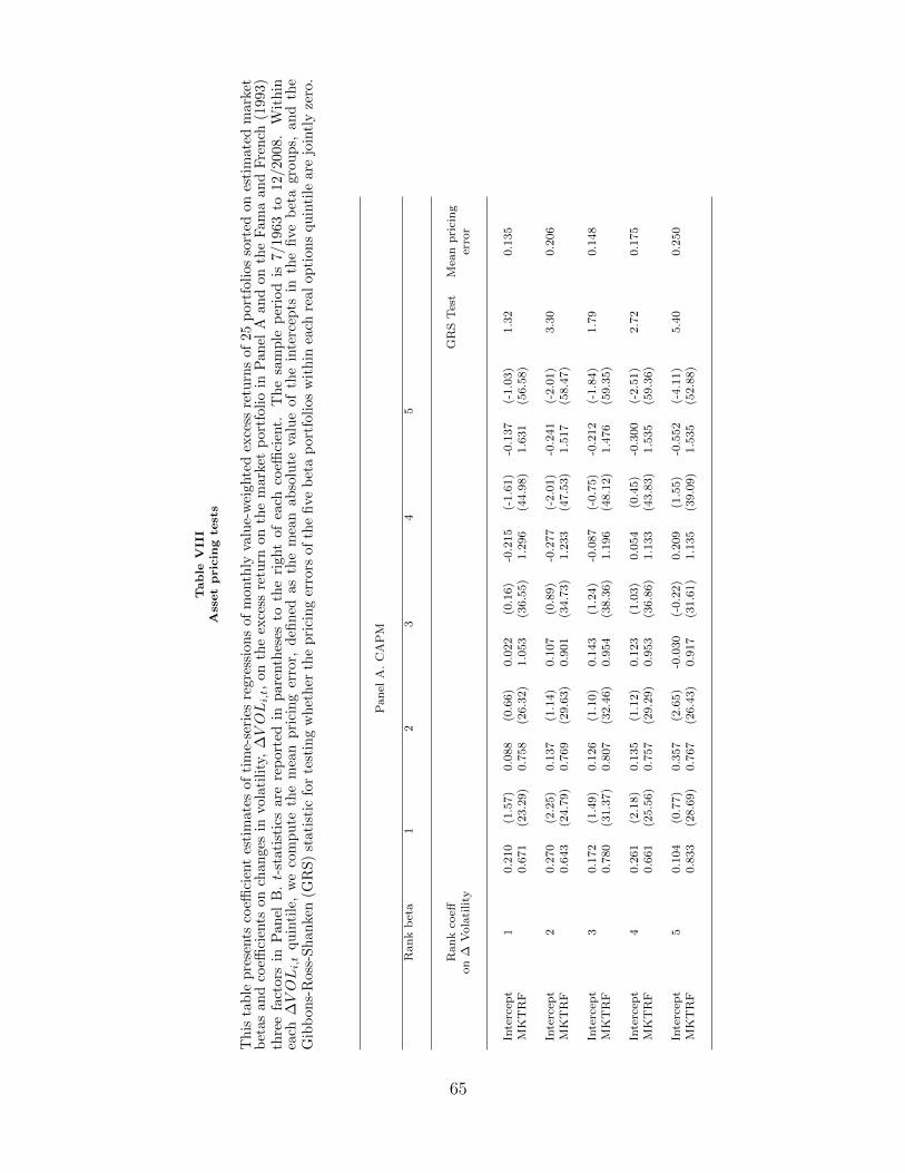
Table

VIII

Assetpricin

gte

sts

Th

ista

ble

pre

sents

coeffi

cien

tes

tim

ates

ofti

me-

seri

esre

gre

ssio

ns

of

month

lyva

lue-

wei

ghte

dex

cess

retu

rns

of

25

port

foli

os

sort

edon

esti

mate

dm

ark

etb

etas

and

coeffi

cien

tson

chan

ges

invo

lati

lity

,∆VOLi,t,

on

the

exce

ssre

turn

on

the

mark

etp

ort

foli

oin

Pan

elA

an

don

the

Fam

aan

dF

ren

ch(1

993)

thre

efa

ctor

sin

Pan

elB

.t-

stat

isti

csar

ere

por

ted

inp

are

nth

eses

toth

eri

ght

of

each

coeffi

cien

t.T

he

sam

ple

per

iod

is7/1963

to12/2008.

Wit

hin

each

∆VOLi,t

qu

inti

le,

we

com

pu

teth

em

ean

pri

cin

ger

ror,

defi

ned

as

the

mea

nab

solu

teva

lue

of

the

inte

rcep

tsin

the

five

bet

agro

up

s,an

dth

eG

ibb

ons-

Ros

s-S

han

ken

(GR

S)

stat

isti

cfo

rte

stin

gw

het

her

the

pri

cin

ger

rors

of

the

five

bet

ap

ort

foli

os

wit

hin

each

real

op

tion

squ

inti

leare

join

tly

zero

.

Pan

elA

.C

AP

M

Ran

kb

eta

12

34

5

Ran

kco

effG

RS

Tes

tM

ean

pri

cin

gon

∆V

ola

tility

erro

r

Inte

rcep

t1

0.2

10

(1.5

7)

0.0

88

(0.6

6)

0.0

22

(0.1

6)

-0.2

15

(-1.6

1)

-0.1

37

(-1.0

3)

1.3

20.1

35

MK

TR

F0.6

71

(23.2

9)

0.7

58

(26.3

2)

1.0

53

(36.5

5)

1.2

96

(44.9

8)

1.6

31

(56.5

8)

Inte

rcep

t2

0.2

70

(2.2

5)

0.1

37

(1.1

4)

0.1

07

(0.8

9)

-0.2

77

(-2.0

1)

-0.2

41

(-2.0

1)

3.3

00.2

06

MK

TR

F0.6

43

(24.7

9)

0.7

69

(29.6

3)

0.9

01

(34.7

3)

1.2

33

(47.5

3)

1.5

17

(58.4

7)

Inte

rcep

t3

0.1

72

(1.4

9)

0.1

26

(1.1

0)

0.1

43

(1.2

4)

-0.0

87

(-0.7

5)

-0.2

12

(-1.8

4)

1.7

90.1

48

MK

TR

F0.7

80

(31.3

7)

0.8

07

(32.4

6)

0.9

54

(38.3

6)

1.1

96

(48.1

2)

1.4

76

(59.3

5)

Inte

rcep

t4

0.2

61

(2.1

8)

0.1

35

(1.1

2)

0.1

23

(1.0

3)

0.0

54

(0.4

5)

-0.3

00

(-2.5

1)

2.7

20.1

75

MK

TR

F0.6

61

(25.5

6)

0.7

57

(29.2

9)

0.9

53

(36.8

6)

1.1

33

(43.8

3)

1.5

35

(59.3

6)

Inte

rcep

t5

0.1

04

(0.7

7)

0.3

57

(2.6

5)

-0.0

30

(-0.2

2)

0.2

09

(1.5

5)

-0.5

52

(-4.1

1)

5.4

00.2

50

MK

TR

F0.8

33

(28.6

9)

0.7

67

(26.4

3)

0.9

17

(31.6

1)

1.1

35

(39.0

9)

1.5

35

(52.8

8)

65

Pan

elB

.F

am

a-F

ren

chth

ree-

fact

or

mod

el

Ran

kb

eta

12

34

5

Ran

kco

effG

RS

Tes

tM

ean

pri

cin

gon

∆V

ola

tility

erro

r

Inte

rcep

t1

0.1

18

(0.9

4)

-0.0

47

(-0.3

8)

-0.0

72

(-0.5

8)

-0.1

51

(-1.2

2)

0.0

21

(0.1

7)

0.5

80.0

82

MK

TR

F0.7

26

(24.8

6)

0.8

45

(28.9

6)

1.0

90

(37.3

2)

1.2

15

(41.6

1)

1.4

09

(48.2

4)

HM

L0.1

71

(3.8

4)

0.2

56

(5.7

1)

0.1

62

(3.6

1)

-0.1

48

(-3.3

1)

-0.3

80

(-8.4

8)

SM

B-0

.046

(-1.1

8)

-0.0

97

(-2.4

7)

0.0

33

(0.8

3)

0.2

11

(5.3

4)

0.6

13

(15.5

2)

Inte

rcep

t2

0.1

34

(1.2

2)

-0.0

06

(-0.0

6)

-0.0

20

(-0.1

8)

-0.2

87

(-2.5

9)

-0.1

02

(-0.9

2)

1.8

10.1

10

MK

TR

F0.7

15

(27.3

3)

0.8

62

(32.9

4)

0.9

93

(37.9

6)

1.1

96

(45.6

9)

1.3

29

(50.7

9)

HM

L0.2

46

(6.1

3)

0.2

72

(6.7

7)

0.2

47

(6.1

4)

-0.0

11

(-0.2

7)

-0.3

29

(-8.2

0)

SM

B-0

.033

(-0.9

3)

-0.1

04

(-2.9

3)

-0.1

35

(-3.8

1)

0.1

78

(5.0

2)

0.5

11

(14.4

5)

Inte

rcep

t3

0.1

12

(1.0

3)

0.0

14

(0.1

2)

0.0

20

(0.1

8)

-0.1

65

(-1.5

1)

-0.1

46

(-1.3

4)

1.0

30.0

91

MK

TR

F0.8

06

(31.2

5)

0.9

05

(35.0

9)

1.0

24

(39.7

0)

1.1

91

(46.1

7)

1.3

37

(51.8

4)

HM

L0.1

04

(2.6

4)

0.2

30

(5.8

2)

0.2

27

(5.7

3)

0.1

12

(2.8

2)

-0.1

89

(-4.7

8)

SM

B0.0

09

(0.2

7)

-0.1

84

(-5.3

0)

-0.0

48

(-1.3

8)

0.1

81

(5.1

8)

0.4

50

(12.9

1)

Inte

rcep

t4

0.1

09

(0.9

9)

0.0

36

(0.3

3)

0.0

15

(0.1

3)

-0.0

69

(-0.6

3)

-0.2

34

(-2.1

3)

1.2

10.0

93

MK

TR

F0.6

93

(26.7

7)

0.8

50

(32.7

9)

1.0

16

(39.2

3)

1.1

80

(45.5

6)

1.3

57

(52.3

9)

HM

L0.2

46

(6.1

8)

0.2

06

(5.1

9)

0.2

01

(5.0

6)

0.2

11

(5.3

2)

-0.2

14

(-5.4

0)

SM

B0.1

68

(4.7

8)

-0.1

91

(-5.4

4)

-0.0

50

(-1.4

3)

0.0

49

(1.3

8)

0.6

13

(17.5

0)

Inte

rcep

t5

0.0

67

(0.5

2)

0.1

91

(1.5

0)

-0.1

90

(-1.4

9)

0.1

01

(0.8

0)

-0.4

93

(-3.8

7)

4.0

70.2

08

MK

TR

F0.8

15

(27.1

2)

0.8

45

(28.1

4)

1.0

06

(33.5

1)

1.1

57

(38.5

3)

1.3

65

(45.4

6)

HM

L0.0

42

(0.9

1)

0.2

94

(6.4

0)

0.2

94

(6.3

8)

0.1

72

(3.7

4)

-0.2

00

(-4.3

3)

SM

B0.1

49

(3.6

8)

0.0

02

(0.0

6)

-0.0

54

(-1.3

3)

0.1

19

(2.9

3)

0.5

91

(14.5

5)

66

Table IXTime Series Regressions

Panel A presents regressions of aggregate (value-weighted) monthly excess return on aggregate volatility andmonth-to-month change in aggregate volatility. Aggregate volatility and change in it refers to the volatility of thevalue-weighted monthly return on all listed stocks. Panel B presents regressions of firm-level excess returns onchanges in aggregate volatility and the Fama and French (1993) three factor returns (MKTRF, HML, and SMB).Panel C presents regressions of firm-level excess returns on changes in aggregate volatility and the Fama andFrench (1993) three factor returns for subsamples of firms grouped by measures of investment opportunities andby measures of flexibility. Only the coefficients on the change in volatility are reported. The last column reportsthe difference between the estimated coefficients on the change in aggregate volatility between the extreme realoptions groups. The sample period is 7/1963 to 12/2008. t-statistics are reported in parentheses. In Panel A,t-statistics are obtained using Newey-West autocorrelation and heteroskedasticity-consistent standard errors. Weestimate panel regressions in Panels B and C and cluster standard errors by month.

Panel A. Dependent variable - aggregate excess return

Aggregate volatility -3.06(-8.57)

∆ Aggregate volatility -3.88(-8.65)

R2 0.118 0.122

# Observations 540 539

Panel B. Dependent variable - firm-level excess return

∆ Aggregate volatility -6.87 -2.33 0.01(-3.36) (-1.02) (0.00)

MKTRF 1.18 1.08(8.93) (5.67)

HML 0.23(0.98)

SMB 1.27(6.12)

R2 0.010 0.040 0.058

# Observations 3,040,952 3,040,952 3,040,952

67

Panel C. Dependent variable - firm-level excess return. By real option groups

Ranking 1 2 3 4 5 5-1

Book assets

∆ Aggregate volatility 0.460 0.205 -0.037 -0.250 -0.175 -0.635(4.94) (4.65) (-1.05) (-6.84) (-7.50) (-6.61)

Age

∆ Aggregate volatility 0.226 0.564 0.137 0.005 -0.244 -0.470(3.15) (8.71) (2.49) (0.14) (-10.37) (-6.22)

RD/ assets

∆ Aggregate volatility 0.004 0.405 0.400 0.809 0.719 0.715(0.05) (4.06) (3.98) (5.82) (4.05) (3.67)

Future sales growth

∆ Aggregate volatility 0.117 0.000 0.085 0.355 0.672 0.555(1.65) (0.01) (1.56) (5.77) (8.25) (5.14)

Earnings convexity

∆ Aggregate volatility 0.095 -0.086 -0.082 0.393 0.349 0.254(2.25) (-1.87) (-1.50) (6.19) (4.23) (2.74)

Sales convexity

∆ Aggregate volatility 0.113 -0.044 0.105 0.013 0.265 0.152(2.86) (-1.10) (1.91) (0.22) (2.52) (1.35)

Union membership

∆ Aggregate volatility 0.141 0.496 0.312 -0.683 -0.509 -0.650(2.24) (3.24) (2.11) (-6.94) (-4.05) (-4.62)

68