Real Options valuation on Six Sigma projects

Real Options valuation on Six Sigma projects

Fernando

Sánchez-Contador de Ros

Master’s Degree Project Tokyo, Japan February 2015

Real Options valuation on Six Sigma projects Page 1

Summary

Economist and financial institutions have long being using option analysis but executives still use the traditional methods for valuing investments (net present value). According to Miller and Park [1], these methods require the assumption of certainty of project cash flows, but fail when used to evaluate strategic investments where payoff is uncertain or at risk. Being uncertainty one of the major issues of long duration projects, practitioners usually use high risk project ratios in order to ensure the viability of the projects. By doing so the threshold that a project has to exceed in order to become viable is sometimes too high, making the company lose potential benefits or market advantages.

This study wants to better understand Real Option Analysis, its application into Six Sigma project evaluation models and the added value obtained by the managerial flexibility that the real options offer. To do so it reviews three real option models: (1) Binomial lattice, (2) Pentanomial lattice, and (3) staged R&D model and then compares the results obtained by valuating the same project using the three different approaches and the traditional NPV.

With the numerical demonstrations we see that the staged R&D model needs a further adaptation to be able to fully compare its numerical results with the other two models. Also find that Real Option models are still hard to include in the practitioners tool kit due to the necessity to adapt or create an specific model for each individual project.

Master Thesis


Index SUMMARY ___________________________________________________ 1

INDEX _______________________________________________________ 3

1. INTRODUCTION ___________________________________________ 5 Objectives .................................................................................................................. 5

2. THEORETICAL INTRODUCTION ______________________________ 7 Real Options .............................................................................................................. 7 Six Sigma Improvement projects .............................................................................. 8

3. MODELS __________________________________________________ 9 Binomial model .......................................................................................................... 9 Pentanomial model ................................................................................................. 11 Staged R&D model ................................................................................................. 13

4. A NUMERICAL DEMONSTRATION ___________________________ 16 Procedure ................................................................................................................ 16 Results ..................................................................................................................... 19

CONCLUSIONS ______________________________________________ 21

IMPACT AND FURTHER RESEARCH ____________________________ 22

ACKNOWLEDGEMENTS _______________________________________ 23

REFERENCES _______________________________________________ 24

ANNEX: PROGRAMING CODE __________________________________ 25 Binomial model ........................................................................................................ 25 Pentanomial model ................................................................................................. 28 Staged R&D model ................................................................................................. 34


1. Introduction

As pointed out by Pande et al. [2], good project selection is itself a process and if properly carried out, the potential benefits of Six Sigma can improve substantially. Despite of that, there is not a unique method to evaluate a project. This makes most practitioners rely on deterministic approaches and their industry expertise to decide whether to go ahead with the project or not.

Despite the flexibility and benefits that real options could add to six sigma project evaluation, there is still not a standard methodology to apply real options to six sigma projects. Giving us the opportunity to be among the first ones to find this method. Since Real Option Analysis is still an unknown methodology for most practitioners we hope that this practical oriented research encourages more of them to include/consider this powerful tool to value their investments.

Real Option Analysis explicitly acounts for the value of future flexibility in decision-making (Trigeorgis [3]). The option values of the projects not only act as a real value of the project, but also augment the flexibility in deision making.

Objectives

Our goal is to find a better way for practitioners to valuate Six Sigma projects taking into account uncertainties existing in the market and the flexibility that they generate for project managers.

This research wants to adapt different Real Option Analysis methods to evaluate them to the same project, that develops stochastically over time, when the decision to invest can be postponed, and to be able to compare the different information that they provide for the practitioners in order to give them a better understanding of the project’s value and its flexibility.


2. Theoretical Introduction

Real Options

The term “real options” was coined by Steward Myers [4]. He asserted that the value of a firm includes the real assets in place plus the present value of options to make further investments in the future. These future investment opportunities are exercised at the discretion of the firm, just as options on trade are executed only when it is profitable to do so.

Copeland and Antikarov [5] have formally defined real option as: “A real option is the right, but not the obligation, to take an action at a predetermined cost called the exercise price, for a predetermined period of time”.

With real options, an alternative becomes available with a business investment opportunity. The initial investment, which is usually pertaining a tangible asset such as capital equipment, buys the prospective opportunity to continue, expand, contract, abandon, … the use of the asset when it is favourable to do so, but it does not carry the obligation to realize some losses when unfavourable conditions occur.

Real options are categorized, by Trigeorgis [3], in the next types: ! Defer: gives the opportunities to delay investment until more information is available

or skill is acquired. ! Abandon: once the expected payoffs diminish to the point where the project is no

longer facing a potential business opportunity, the management has the opportunity to cease the project preventing future losses.

! Switch inputs, outputs or risky assets: giving the opportunity to change some of the assets in the project.

! Alter operating scale: expanding or contracting the scale of investment in terms of resources in accordance the the availability of new information and the new expected outcome.

! Growth options: provide the executives the opportunity to follow on investments, many of which may not be anticipated at the time of initiating the project.

! Staged investment: giving the opportunity to stay/enter a market/project without committing all of the economic resources before the expected outcome is within the objectives of the organization.

The addition of real options to the project has the potential to improve managerial decision making. It systematically organizes the analysis, helps to reformulate the problem to provide additional insight into the investment opportunity and to reveal more of its caracteristics, distinguishes between alternative investment options which are included in the single investment opportunity, improves communication between executives, and provides a better interface for capital investment, decision making, strategic management and long range staged planning.

Master Thesis

Real options approach incorporates a learning model, such that practitioners make better and more informed strategic decisions when some uncertainties are resolved through the stages of the project. On the other hand, dicounted cash flow analysis assumes a static investment decision and assumes that srategic decisions are made initially with no alternative to choose other pathways or options in future stages of the project. A big part of the added value given by real options is that force managers to ad flexibility to their investments from the conceiving of the project, arising a lot of usefull insight in their strategy planning.

Six Sigma Improvement projects

“Six Sigma is a comprehensive and flexible system for achieving, sustaining and maximizing business success. Six Sigma is uniquely driven by close understanding of customer needs, disciplined use of facts, data and statistical analysis and diligent attention to managing, improving and reinventing business processes.” Pande et al. [2].

The main keys that lead Six Sigma projects to success are: the high involvement of the managers in the improvement process, the utilization of trained improvement specialists (belts), the use of clearly defined performance metrics and measurements (costs, quality, methods,…), the implementation with a systematic procedure, define, measure, analyse, improve and control (DMAIC), and the project selection and prioritization.

At macro level the investments in Six Sigma projects can be viewed as capital investment projects. These share three common characteristics: (1) they are partially or completely irreversible, (2) there is uncertainty over the future rewards from the investment, and (3) the managers have some leeway about timing of the investment (Dixit and Pindyck [6]).

Six Sigma projects are carried out in project stages (DMAIC/DMADV). The rewards are realized only upon the completion of the project. On the other hand, the resources needed for the project are identified before each of the stages (DMAIC). The project leader is not obliged to make all the expenditures before the first stage (Define) and can asses on how to continue with the project once new information comes available through time.

The common bounds between Six Sigma and capital investment projects like their organization in clearly defined stages and the benefits obtained by selecting the most suitable project makes for a great opportunity for the use of Real Option Analysis to model the project’s value.


3. Models

In this section the different models used to value the quality improvement projects are described.

Each one of the models selected implies a different level of difficulty for the management. By studying these models and comparing the results obtained we want to give a better insight to practitioners seeking to use Real Option Analysis to value and take better decisions when facing quality improvement projects.

Binomial model

This is a binomial lattice-based [13], by Padhy and Sahu [7], the model generates a binomial tree starting from the current value of the selected variable and expands through the option life of the project. By doing so, demonstrates alternative possibilities over time [6].

To model uncertainties through binomial method one of the major issues faced is the selection of the input parameters. The parameters that are required for the implementation of this model into a Six Sigma project are:

• Current value of the underlying asset (S0). • Strike price/option’s exercise price, which for Six Sigma projects represents the

cost of all the investments made for the project life cycle. • Option life of the project (T). • Interval size (δt) of the time steps between different stages. • Volatility of the asset value (σ), which is the variability of the total value of the asset

over its lifetime. • Risk free interest rate/rate of return on a risk less asset during the life of the option

(r).

With the above mentioned parameters we are able to calculate the up and down factors, which are the function of the underlying asset, that is modelled following a Geometric Brownian Motion, and the risk neutral probability.

Up factor:

Down factor:

u = eσ δt (Eq. 3.1)

Master Thesis

The assumption that the down factor is the inverse of the up factor significantly diminishes the growth rate of the tree.

Risk neutral probability:

Then the binomial tree is built based on the number of time increments selected and starting from S0 moves up S0u with probability p or down to S0d with probability 1-p, repeating for all the other nodes as exemplified in figure 3.1. Calculating the asset values at each node of the tree.

Fig. 3.1. Binomial tree. [7]

Afterwards, by using a process called backward induction, which starts at the right side of the binomial tree, we calculate the option value at each node of the tree as follows.

d = 1u

(Eq. 3.2)

p = erδt−du−d (Eq. 3.3)

S0u2 = [p(S0u

3)+ (1− p)(S0u2d)]e−rΔt (Eq. 3.4)


Obtaining the project value once the final option values of the project are calculated. The option value added by the option for waiting can be obtained by subtracting the end value calculated with the traditional NPV.

Pentanomial model

In this model we assume that two variables affect the outcome of the project. We will use the two-state Kamrad and Richken [8], approach since it can be used to find the option value and optimal strategy in the Six Sigma project.

It proposes a pentanomial lattice structure with two variables S1 and S2 that have a joint density that follows a bivariate lognormal distribution, with correlation ρ.

For variable i (i=1,2) we have and instantaneous mean (µi):

Where r is the risk free interest rate and σ2 is the instantaneous variance.

In each step the values of the two variables may increase, decrease or stay stable. The five possible different paths are as in table Fig. 3.2.

S1 S2 Probability

u1 u2 p1

u1 d2 p2

1 1 p3

d1 u2 p4

d1 d2 p5

Fig. 3.2. Variable jump amounts and probabilities.

µi = r −σ i2

2 (Eq. 3.5)

Master Thesis

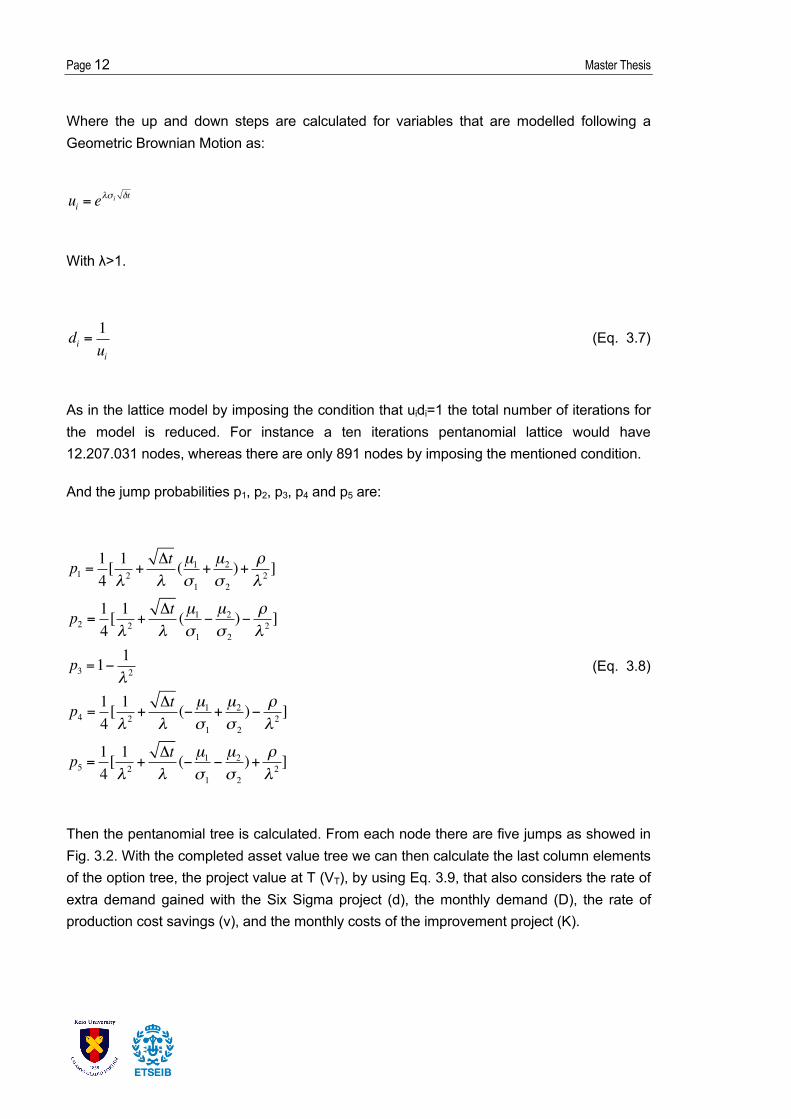
Where the up and down steps are calculated for variables that are modelled following a Geometric Brownian Motion as:

With λ>1.

As in the lattice model by imposing the condition that uidi=1 the total number of iterations for the model is reduced. For instance a ten iterations pentanomial lattice would have 12.207.031 nodes, whereas there are only 891 nodes by imposing the mentioned condition.

And the jump probabilities p1, p2, p3, p4 and p5 are:

Then the pentanomial tree is calculated. From each node there are five jumps as showed in Fig. 3.2. With the completed asset value tree we can then calculate the last column elements of the option tree, the project value at T (VT), by using Eq. 3.9, that also considers the rate of extra demand gained with the Six Sigma project (d), the monthly demand (D), the rate of production cost savings (v), and the monthly costs of the improvement project (K).

ui = eλσ i δt (Eq. 3.6)

di =1ui

(Eq. 3.7)

p1 =14[ 1λ 2

+Δtλ(µ1σ1

+µ2σ 2

)+ ρλ 2]

p2 =14[ 1λ 2

+Δtλ(µ1σ1

−µ2σ 2

)− ρλ 2]

p3 =1−1λ 2

p4 =14[ 1λ 2

+Δtλ(− µ1σ1

+µ2σ 2

)− ρλ 2]

p5 =14[ 1λ 2

+Δtλ(− µ1σ1

−µ2σ 2

)+ ρλ 2]

(Eq. 3.8)


From here backward discounting is applied in the same way applied at the binomial model and as showed in Eq. 3.4 but by multiplying each possible jump by its jump probability as calculated in Eq. 3.8.

The option value added by the option for waiting can be obtained by the same means as in the binomial model.

Staged R&D model

This model was originally presented by Huczermeier-Loch [9] for valuing R&D projects and then adapted by M.Tkác and S.Lyocsa [10] for Six Sigma projects.

It assumes that the project is divided into T consecutive discrete project stages, t=1,2,…,T and before every stage the project leader has the option to abandon, continue, improve or shrink the project.

When, after receiving new information project expectations do not change significantly the option to continue is exercised and the project has some continuation costs (ct). While, when the expectations change, management may decide to improve when increased, paying some improvement costs (αt), and to shrink when decreased, paying some shrinking costs (dt). When exercising the option to increase the expectations for the project should also be increased, and decreased when exercising the shrinking option.

Expectations refer to critical customer parameters (CCP). All the stages of the project can be modelled using the level of CCP. We will refer as CCP as the state of the system (it) which for all t will be bound in the interval, It=(a1,a2). Being It the space of states, a1 the lower boundary and a2 the upper boundary. The space of states will remain constant for all the states.

To model the transition probability from one state to the other states due to the new information available at the next step we use function Eq. 3.10. Which is equivalent to model project uncertainty by using a normally distributed random variable N(it,σ2) with probability density Eq. 3.10.

VT =max(0,dS1,tD+ vS2,tD−K ) (Eq. 3.9)

f ( j) = 1σ 2π

e−

1

2( j−itσ)2

(Eq. 3.10)

Master Thesis

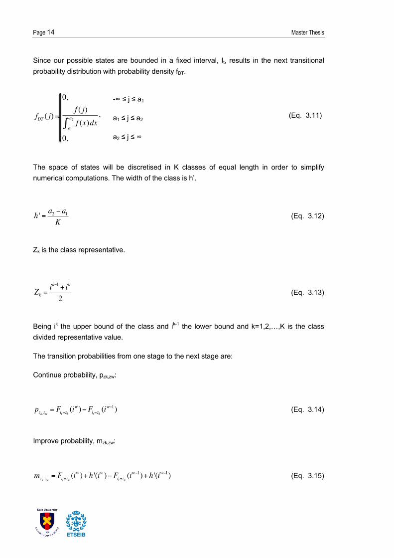
Since our possible states are bounded in a fixed interval, It, results in the next transitional probability distribution with probability density fDT.

The space of states will be discretised in K classes of equal length in order to simplify numerical computations. The width of the class is h’.

Zk is the class representative.

Being ik the upper bound of the class and ik-1 the lower bound and k=1,2,…,K is the class divided representative value.

The transition probabilities from one stage to the next stage are:

Continue probability, pzk,zw:

Improve probability, mzk,zw:

0,f ( j)f (x)dx

a1

a2∫,

0,

(Eq. 3.11) fDT ( j) =

h ' = a2 − a1K

(Eq. 3.12)

Zk =ik−1 + ik

2 (Eq. 3.13)

pzk ,zw = Fit=zk (iw )−Fit=zk (i

w−1) (Eq. 3.14)

mzk ,zw= Fit=zk (i

w )+ h '(iw )−Fit=zk (iw−1)+ h '(iw−1) (Eq. 3.15)

-∞ ≤ j ≤ a1

a1 ≤ j ≤ a2

a2 ≤ j ≤ ∞


Shrink probability, szk,zw:

Where w=1,2,…,K represents the kth class in the next stage, Fit=zk(iw) is the cumulative distribution function of a doubly truncated normal distribution with mean it.

Then the value of the project, V, is calculated using the recursive dynamic stochastic programming approach, where:

For t=T-1

For t<T-1

Where π(zw) represents the payoff function as in Eq. 3.9.

The valued added to the project by the included options can be calculated as:

V(zt=1)-V(zt=1)*

Where V(zt=1)* is calculating by only considering the option to continue with the project.

szk ,zw = Fit=zk (iw )− h '(iw )−Fit=zk (i

w−1)− h '(iw−1) (Eq. 3.16)

AO : 0

CO :−cT−1 + w=1W pzk ,zwπ (zw )∑ ·e−rΔt

IO :−cT−1 −αT−1 + w=1W pzk ,zwπ (zw )∑ ·e−rΔt

SO :−cT−1 + dT−1 + w=1W pzk ,zwπ (zw )∑ ·e−rΔt

(Eq. 3.17)

AO : 0

CO :−cT−1 + w=1W pzk ,zwV (zw )∑ ·e−rΔt

IO :−cT−1 −αT−1 + w=1W pzk ,zwV (zw )∑ ·e−rΔt

SO :−cT−1 + dT−1 + w=1W pzk ,zwV (zw )∑ ·e−rΔt

(Eq. 3.18) V (zk ) =MAX

V (zk ) =MAX

Master Thesis

4. A numerical demonstration

To compare the results obtained by using the three different models, binomial model, pentanomial model and staged R&D model we used the price and production costs of the asset as stochastic distributions.

S1,0 represents the price of the asset at t=0 and is 1.500. S2,0 represents the production cost of the asset and at t=0 and is 500. Both variables have a volatility of 0,3. And have a correlation of 0,2. The time duration of the project is 15 months with time steps of 1 month. The demand of the product is 1.000 units per moth. The risk free interest rate is 3 %. The cost of implementing a quality improvement program is 20.000. The rate of cost savings when the program is implemented is 2 % and the rate of extra demand if quality improvement is implemented is 3 %.

Procedure

At the last stage of all the models Eq. 3.9 is used to calculate the value of the project with the current variable state.

In order to be able to use Eq. 3.9 with the binomial model, we need to define the values for the second variable at t=T, since the first variable is modelled following a Geometric Brownian Motion distribution. We ran different test cases with the values as showed in fig. 4.1.

case S2,T case S1,T

1 24.701,22 5 74.103,67

2 2.240,84 6 6.722,53

3 111,57 7 334,70

4 10,12 8 30,36

Fig. 4.1. Binomial test input variables.

S1,T and S2,T represent the achieved value of variables S1 and S2 at time T, when it approximated as showed in fig. 4.1.


In the pentanomial model there is no need to adapt or add further information in order to be able to calculate the value of the Six Sigma project. Since it already accounts for the distribution of both S1 and S2 there is only one numerical case made with this model, case number 9.

In the staged R&D model we add an additional dimension to the project, the critical customer parameter. This parameter will be modelled as a customer satisfaction index. Being 0 its lowest possible value and 8 its highest. Due to the relation between customer satisfaction and demand, the rate of extra demand (d) will have the next values in the staged R&D model, which vary, according to the CCP level achieved in each situation as showed in fig. 4.2.

CCP Level d

8 4 %

7 4 %

6 3 %

5 3 %

4 2 %

3 2 %

2 1 %

1 1 %

Fig. 4.2. Rates of extra demand in the R&D model.

The level at which the Six Sigma project improves the rate of extra demand suffers from a bigger loss when the customer satisfaction level achieved is low, since the impact that unsatisfied costumers have on other costumers is bigger than the one produced by satisfied costumers. Also and to be consistent with general situations where an organization decides to implement a Six Sigma quality improvement project, we will fix the starting customer satisfaction level at 1 (the lowest) for t=0.

In order to evaluate the same options as in the binomial and pentanomial models only the option to abandon and to continue will be considered in Eq. 3.17 and Eq. 3.18.

Master Thesis

The test cases for the staged R&D model have been done with variables S1,T and S2,T at the levels provided in Fig. 4.3.

case S1,T S2,T

10 1.500 24.701,22

11 1.500 2.240,84

12 1.500 111,57

13 1.500 10,12

14 74.103,67 500

15 6.722,53 500

16 334,70 500

17 30,36 500

Fig. 4.3. R&D model input variables.


Results

case With option Without option Option value

1 336.988,53 336.988,53 0,00

2 59.026,33 59.026,33 0,00

3 33.918,38 33.895,72 22,66

4 33.075,57 32.978,69 96,88

5 1.372.952,46 1.372.952,46 0,00

6 122.122,55 122.122,55 0,00

7 5.515,60 5.345,07 170,53

8 3.757,67 3.492,81 264,87

9 27.361,91 27.135,56 226,35

10 0,00 1.600,41 -

11 0,00 845,51 -

12 0,00 773,94 -

13 0,00 770,53 -

14 0,00 39.693,14 -

15 0,00 3.585,60 -

16 0,00 162,55 -

17 0,00 - -

Fig. 4.4. Results.

Master Thesis

As seen through tests 1 to 8, the option value is 0,00 when the guessed values for the non lattice variable are high, cases 1 and 2 (S2,T), and 5 and 6 (S1,T). On the other hand, the binomial model gives some value to the option when the guessed values are low, cases 3, 4, 6 and 7.

Looking at the results from the pentanomial model we find out that by considering that both variables follow a stochastic distribution over time, the added value option of the project is higher. This result could be expected since the model takes into account the distribution for both variables, instead of using an approximated guess for the expected value at T.

In the staged R&D model, by including the CCP we see that the value of the project with option to abandon is always 0. That means that by starting at the lowest level of CCP, and despite of all the different sets of asset price and production costs selected for the different numerical cases, the project should never be implemented, according to the results obtained in this model. This is a big contrast with the results obtained with the other two models. In order to make the comparison possible, it may be necessary to use a different technique to select the parameter values. Also the inclusion of a CCP value in the lattice models may help reaching closer results when evaluating Six Sigma projects using the different models.


Conclusions

Real option Analysis is a valid approach in order to valuate Six Sigma improvement projects and the former could get significantly benefited by the standardization of the use of real option in the project selection step of the process.

The results obtained, specially the ones from the binomial and pentanomial model have been as expected, the option value in the pentanomial model is generally higher than the ones obtained in the binomial.

Regarding the staged R&D approach studied, we believe that it still needs a bigger adaptation in order to be able to be implemented fully as the other two models. Nevertheless it shows significant potential for Six Sigma improvement projects due to the use of a standardize parameter, one of the keys to success of Six Sigma (use of clearly defined performance metrics and measurements) to be able to keep track of the improvement process without loosing focus on the key elements that need to be improved.

We believe that there is a need for further development of real option models for practitioners to start using them in a more usual basis, instead of using the traditional discounted cash flow techniques. One of the main issues faced is the need to adapt or create a new model that suits each specific project.

Master Thesis

Impact and further research

This thesis aimed to take real options a step closer to managers. With the current state of the art, at least in quality management models, we think that more customized models need to be developed in this area.

Some of the further research that can be done in this area include the use of more options to broader the impact and the flexibility that they bring into the projects. Also it would be interesting to combine the customer focus parameter of Six Sigma projects into the lattice models.


Acknowledgements

I would like to give special thanks to professor Junichi Imai from Keio University, who welcomed me into his laboratory and guided me through my research.

Master Thesis

References

[1] Miller, L.T., Park, C.S., 2002. Decision making under uncertainty-real option to the rescue. The Engineering Economist 47 (2), 105-150.

[2] Pande PS, Neuman RP, Cavanagh RR. The Six Sigma Way: How GE, Motorola and other Top Companies are Honing their Performance. McGraw-Hill: New York, 2000.

[3] Trigeorgis, L., 1996. Real Options. MIT Press, Cambridge, MA.

[4] Myers, S.C. 1977. Determinants of corporate borrowing. Journal of Financial Economics 5: 147-175.

[5] Copeland, T., and Antikarov, V. 2001. Real options: A practitioner’s guide. New York: Texere.

[6] Dixit, A.K., Pindyck, R.S., 1993. Investment under Uncertainty. Princeton University Press, Princeton, NJ.

[7] R.K. Padhy, S. Sahu. A Real Option based Six Sigma project evaluation and selection model. International Journal of Project Management 29 (2011) 1091-1102.

[8] Kamrad, B., and P. Ritchken. 1991. Multinomial approximating models for options with k state varaibles. Management Science 37 (12): 1640-1653.

[9] Huchzermeier A, Loch Ch. Project management under risk: Using the real options approach toe evaluate flexibility in R&D. Management Science 2001; 47 (1): 85-101.

[10] M. Tkác and S. Lyócsa. On the evaluation of six sigma projects. Quality and Reliability Engineering International 2009, 26 115-124.

[11] Harriet Balck Nembhard and Mehmet Aktan. Real Option in Engineering Design, Operations and Management.

[12] Junichi Imai. An alternative Lattice approach for multidimensional Geometric Brownian Motions. 1997, technical report 97-5.

[13] Cox, J. C., S. A. Ross and M. Rubinstein, 1979, “Option Pricing: A Simplified Approach”, Journal of Financial Economics 7 (3), pp. 229-63.


Annex: Programing code

Binomial model

% Binomial model by Padhy and Sahu

% Initialize variables

clear

tt=15; % time intervals

tint=1; % length of time interval

r=0.03; % risk free interest rate

o=0.3; % standard deviation price

ben=1500; % value of the price at t=0

V2=500; % production cost at T

d=0.03; % rate of extra demand

D=1000; % demand per month

v=0.02; % rate of production costs savings

kcost=20000; % monthly cost

F=300000; % fixed production cost per month

up=exp(o*sqrt(tint)); % up jump

down=1/up; % down jump

p=(exp(r*tint)-down)/(up-down);

% Ends initialization

% Calculates the variable through all the time intervals (T)

S(1,1)=ben;

Master Thesis

for t=2:1:tt+1

auxS=zeros(t,1);

auxS(1,1)=S(1,1)*up;

for i=2:1:t

auxS(i,1)=S(i-1,1)*down;

end

clear S;

S=auxS;

clear auxS;

end

% Calculates the option value at T

O=zeros(tt+1,1);

for i=1:1:tt+1

O(i,1)=max(0,d*S(i,1)*D+v*V2*D-kcost);

end

O=O*exp(-r*tint);

clear S;

% Backward calculates the option value from T-1

for t=tt:-1:1

auxO=zeros(t,1);

for i=1:1:t

auxO(i,1)=max((p*O(i,1)+(1-p)*O(i+1,1))*exp(-r*tint),0);

end


clear O;

O=auxO;

clear auxO;

end

Master Thesis

Pentanomial model • Main program

% Two state Kamrad and Ritchken model

clear

% Initialize variables

tt=15; % time stages

tint=1; % time interval lenght

lamda=3/2;

r=0.03; % risk free interest rate

o1=0.3; % standard deviation variable 1

o2=0.3; % standart deviation variable 2

ro=0.2; % correlation between variable 1 and 2

up1=exp(o1*sqrt(tint)); % up jump variable 1

up2=exp(o2*sqrt(tint)); % up jump variable 2

mu1=r-(o1^2)/2; % instantaneous mean variable 1

mu2=r-(o2^2)/2; % instantaneous mean variable 2

% p1-p5 probability for each scenario (+ +, + -, = =, - +, - -)

p1=(1/4)*((1/(lamda^2))+(sqrt(tint)/(lamda))*((mu1/o1)+(mu2/o2))+(ro/(lamda^2)));

p2=(1/4)*((1/(lamda^2))+(sqrt(tint)/(lamda))*((mu1/o1)-(mu2/o2))-(ro/(lamda^2)));

p4=(1/4)*((1/(lamda^2))+(sqrt(tint)/(lamda))*(-(mu1/o1)+(mu2/o2))-(ro/(lamda^2)));

p5=(1/4)*((1/(lamda^2))+(sqrt(tint)/(lamda))*(-(mu1/o1)-(mu2/o2))+(ro/(lamda^2)));

p3=1-p1-p2-p4-p5;

% Fin inicialización


% Programa

S0=1500; % starting value of the price

V0=500; % starting value of the production cost


d=0.03; % rate of extra demand




% Calculates the project value at T as if it where a ninomial model

Sf9=zeros((2*(tt)+1)^2,1);

row=1;

for t2=(tt):-1:-(tt)

for t3=(tt):-1:-(tt)

Sf9(row,1)=max(0,d*S0*(up1^t2)*D+v*V0*(up2^t3)*D-kcost);

row=row+1;

end

end

clear row;

% Adapts the project values from a ninomial model to pentanomial

Sf5=zeros(((tt+1)^2+tt^2),1);

for t2=1:1:((tt+1)^2+tt^2)

Sf5(t2,1)=Sf9((2*(t2-1)+1),1);

end

Master Thesis

clear Sf9;

Sf5=Sf5*exp(-r);

% Backward calculates the project value until t=1

for t2=tt:-1:1

aux=Option5(Sf5,t2,p1,p2,p3,p4,p5,r);

clear Sf5;

Sf5=aux;

clear aux;

end

% npv=ben-inv;

% OptionValue(tt,1)=Sf;

% Sf is the project value • Auxiliar function

function [ B ] = Option5( A,n,p1,p2,p3,p4,p5,ratio )

% Option returns the project value at n-1

B=zeros((n^2+(n-1)^2),1);

m=0;

q=1;

s=0;

r=0;

t=1;

principio=0;

aux=n;

y=0;


P=zeros(5,1);

P(1,1)=p1;

P(2,1)=p2;

P(3,1)=p3;

P(4,1)=p4;

P(5,1)=p5;

for k=1:1:(((n-1)+1)^2+(n-1)^2)

aux2=zeros(5,1);

z=2;

for i=1:1:3

for j=1:1:z

aux2(q,1)=A(j+r+y+principio,1);

q=q+1;

s=s+1/5;

r=floor(s+0.0002);

end

if z>1

z=1;

else

z=2;

end

if i<3

if i<2

Master Thesis

y=n+1;

else

y=2*n+1;

end

else

y=0;

end

end

q=1;

t=t+1;

if t>(aux)

s=0;

r=0;

t=1;

end

m=(m+(1/(aux)));

m1=floor(m+0.0002);

if m1>0.5

principio=principio+aux+1;

m=0;

if aux>(n-1)

aux=n-1;


else

aux=n;

end

end

B(k,1)=dot(aux2,P);

B(k,1)=B(k,1)*exp(-ratio);

clear aux2;

end

end

Master Thesis

Staged R&D model ! Main program:

% Hutchzermeier-Loch (R&D) Dynamic Programming

clear all;

K=8; % Critical costumer parameter levels

a2=8; % Upper boundary CCP

a1=0; % Lower boundary CCP

T=15; % number of periods

h=(a2-a1)/K; % class width

o=3; % standard deviation

r=0.03; % free risk interest rate

V1=30.3628671687066; % value of the price at T

V2=500; % production cost at T

d=zeros(8,1); % rate of extra demand

d(1,1)=0.01;

d(2,1)=0.01;

d(3,1)=0.02;

d(4,1)=0.02;

d(5,1)=0.03;

d(6,1)=0.03;

d(7,1)=0.04;

d(8,1)=0.04;






% Calculating the upper and lower bound of each class

i=zeros(K+1,1);

i(1,1)=a1;

for j=2:1:K+1

i(j,1)=i(j-1,1)+h;

end

% Calculating the class representatives

z=zeros(K,1);

z(1,1)=((i(2,1)-i(1,1))/2)+i(1,1);

for j=2:1:K

z(j,1)=z(j-1,1)+h;

end

% Calculating the Option values at T-1

V=zeros(K,T-1); % Option values for each class at each time

Step=zeros(K,T-1); % 0= Abandon, 1= Continue

CO=zeros(K,1);

aux=K;

for it=z(1,1):h:z(K,1)

COaux=0;

for j=1:1:K

Master Thesis

COaux=COaux+ContinueT(i,j,it,o,a1,a2,V1,V2,d,D,v,kcost);

end

% For each class calculate the option that maximizes the value

CO(aux,1)=COaux*exp(-r);

[V(aux,T-1),Step(aux,T-1)]=whatisbiggercontinue(CO,aux);

aux=aux-1;

end

%Calulating the Option values for t

for t=T-2:-1:1

aux=K;

for it=z(1,1):h:z(K,1)

COaux=0;

for j=1:1:K

COaux=COaux+Continue(i,j,it,o,V,t,a1,a2);

end

% For each class calculate the option that maximizes the value

CO(aux,1)=COaux*exp(-r);

[V(aux,t),Step(aux,t)]=whatisbiggercontinue(CO,aux);

aux=aux-1;

end

end ! Continuation value at T-1

function [ CO ] = ContinueT(i,j,it,o,a1,a2,V1,V2,d,D,v,kcost)

%ContinueT calculates the continuation value of the project at T-1


aux2=(50703919*((pi/2)^0.5)*(erf((a2-it)/o*(2)^0.5)-erf((a1-it)/o*(2)^0.5)))/127095877;

aux=d(j,1)*(V1)*D+v*(V2)*D-kcost;

CO=((1/(o*((2*pi)^(-0.5))))*exp(-0.5*((i(j+1,1)-it)/o)^2)-(1/(o*((2*pi)^(-0.5))))*exp(-0.5*((i(j,1)-it)/o)^2))*aux/aux2;

end ! Continuation value at t < T-1

function [ CO ] = Continue(i,j,it,o,V,t,a1,a2)

%ContinueT calculates the continuation value of the project for t<T-1

aux=V(j,t+1);

aux2=(50703919*((pi/2)^0.5)*(erf((a2-it)/o*(2)^0.5)-erf((a1-it)/o*(2)^0.5)))/127095877;

CO=((1/(o*((2*pi)^(-0.5))))*exp(-0.5*((i(j+1,1)-it)/o)^2)-(1/(o*((2*pi)^(-0.5))))*exp(-0.5*((i(j,1)-it)/o)^2))*aux/aux2;

end ! Comparisson function

function [ V,Step ] = whatisbiggercontinue( CO,aux )

% whatisbigger returns the maximum option value between CO and AO and records which one is taken

Step=0;

if CO(aux,1)>0

V=CO(aux,1);

Step=1;

else

V=0;

end

end

Real Options valuation on Six Sigma projects

Documents

Transcript of Real Options valuation on Six Sigma projects