Real Options

November 5, 2010

By: A V Vedpuriswar

Introduction

¨ Real options are useful under the following conditions:– Contingent investment decisions– High uncertainty– Need to wait for more information– Value lies in future growth options– Flexibility is important– Mid course corrections may be needed as the

scenario unfolds– The pay offs to investments are non linear– Conventional tools fail to capture the upside

potential and trade offs required in strategic decisions.

Problem with NPV

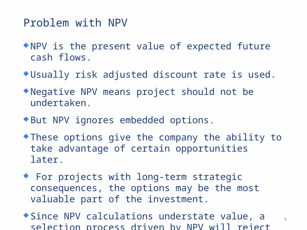
¨ NPV is the present value of expected future cash flows.

¨ Usually risk adjusted discount rate is used.

¨ Negative NPV means project should not be undertaken.

¨ But NPV ignores embedded options.

¨ These options give the company the ability to take advantage of certain opportunities later.

¨ For projects with long-term strategic consequences, the options may be the most valuable part of the investment.

¨ Since NPV calculations understate value, a selection process driven by NPV will reject more potentially profitable projects.

3

Understanding embedded options

¨ A timing option, in the form of a delayed expansion in capacity could create value in a situation of uncertain demand.

¨ Putting up a plant in an overseas market currently fed by exports may generate new growth options.

¨ An exit option in the form of a plant closure increases the value of the investment decision.

¨ By looking at strategic decisions in terms of options and then using information from financial markets to value these options, risk can be greatly reduced.

¨ Oil companies for example can predict the future price of oil through the futures markets.

¨4

Private risks

¨ Decision makers will not be able to draw information from the financial markets for all decisions.

¨ Some uncertainties are insulated from the market mechanism and are specific to a company.

¨ These are ‘private risks’.

¨ But as more and more risks become securitised, the options approach may become more and more feasible.

¨ Securitisation converts illiquid non traded investments into liquid instruments, which are actively traded in the market.

5

The real value of real options

¨ As Amram and Kulatilaka put it: “The real value of real options, we believe, lies not in the output of Black-Scholes or other formulas but in the reshaping of executives’ thinking about strategic investment. By providing objective insight into the uncertainty present in all markets, the real options approach enables executives to think more clearly and more realistically about complex and risky strategic decisions. It brings strategy and shareholder value into harmony.”

6Ref : Amram, Kulatilaka, “ Real Options : Managing strategic investment in an uncertain world”

Real options and risk management

¨ A new business or a major investment in capacity expansion may result in a variety of outcomes that may demand a range of strategic responses.

¨ Plans to change operating or investment decisions later, depending on the actual outcome, must form an integral component of the projections.

¨ Thinking of the investment in terms of options, allows uncertainty to be taken into account.

7

Options are of value only in an uncertain environment.

¨ Investment decisions, whose primary objective is to acquire options, must be made before uncertainties in the environment are resolved.

¨ As Sharp says, “Unlike cash flows, whose value may be positive or negative, option values can never be less than zero, because they can always be abandoned. Embedded options can therefore, only add to the value of an investment. Options are only valuable under uncertainty: if the future is perfectly predictable, they are worthless”.

¨ Ref : Sloan Management Review, Summer 1991.

8

The building blocks of real options

¨ Real options may have complex pay offs.

¨ But the building blocks are simple:– Buy a call option– Write a call option– Buy a put option– Write a put option– Go long on underlying asset– Go short on underlying asset

¨ A call option enables an investor to take advantage of potential good news or high values of the underlying asset.

¨ A put option enables an investor to take advantage of potential bad news or low values of the underlying asset.

¨ A call option is appropriate for a bullish investor.

¨ A put option is ok for a bearish investor.

Understanding Option payoffs

Inputs needed for valuing an option

¨ Current value of underlying asset.

¨ Time to decision date

¨ Investment cost

¨ Strike price

¨ Risk free rate of interest

¨ Volatility of underlying asset

¨ Cash payouts/non capital gains

The Black Scholes Option pricing model

¨ Consider a portfolio of traded securities.

¨ This is called a tracking portfolio.

¨ It has the same pay offs as the option.

¨ Let us impose no arbitrage condition.

¨ The value of the option equals the value of the portfolio as the stock price moves.

¨ This is the basis for Black Scholes model.

Challenges in dynamic tracking

¨ Two features of underlying assets cause tracking error :

– Costs of tracking

– Quality of tracking

Leakages in value

¨ Real assets may generate cash payments similar to a dividend.

¨ Convenience yield may result from holding the asset.

¨ These benefits are available only to the holder of the underlying asset, not to the option holder.

Basis risk

¨ The traded securities in the tracking portfolio may not be perfectly correlated with the value of the option.

¨ The imperfect correlation may be the result of product quality, delivery location, timing, etc.

Private risk

¨ Real options have risks that are not contained in the available set of traded securities.

¨ These private risks are not priced in the financial markets.

Errors/costs in tracking

¨ Infrequent trading

¨ Illiquidity

¨ Costs of coordinating, monitoring and documenting

¨ Infrequent observability

Illustration

¨ A wants to fill in a gap in it product line and has proposed to B that it will invest $ 35 million today for rights to buy B for $ 200 million in three years. The current market value of B is $192 million. Is the deal attractive? Assume Volatility = 30% and r = 5%

¨ S= 192, k= 200, t = 3 years, = 30%, r= 5%

¨ d1 = 0.47, d2 =.47- .3x√3= - .05, N(d1 ) = .6808, N(d2 ) = .4801

¨ C= 192x0.6808 – 200 x e-.15 x 0.4801 = 130.71-82.65 = 48.06

¨ So the price offered is very low.

Ref : Amram, Kulatilaka, “ Real Options : Managing strategic investment in an uncertain world”

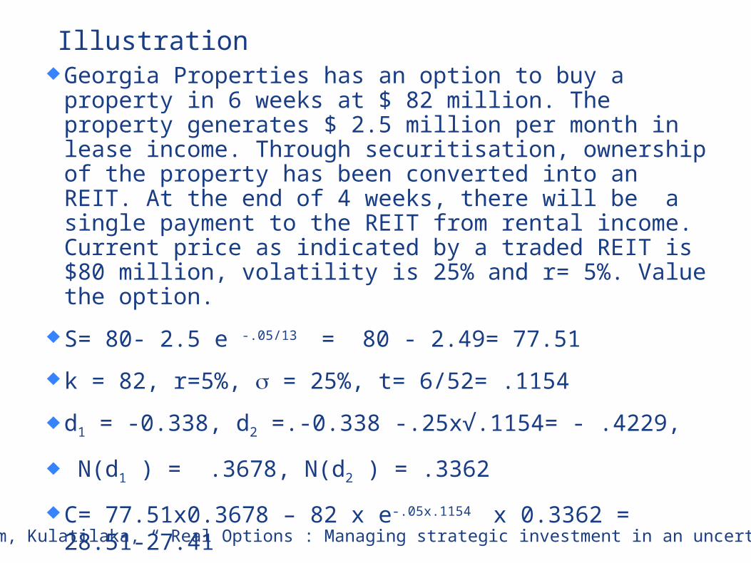
Illustration¨ Georgia Properties has an option to buy a property in 6

weeks at $ 82 million. The property generates $ 2.5 million per month in lease income. Through securitisation, ownership of the property has been converted into an REIT. At the end of 4 weeks, there will be a single payment to the REIT from rental income. Current price as indicated by a traded REIT is $80 million, volatility is 25% and r= 5%. Value the option.

¨ S= 80- 2.5 e -.05/13 = 80 - 2.49= 77.51

¨ k = 82, r=5%, = 25%, t= 6/52= .1154

¨ d1 = -0.338, d2 =.-0.338 -.25x√.1154= - .4229,

¨ N(d1 ) = .3678, N(d2 ) = .3362

¨ C= 77.51x0.3678 – 82 x e-.05x.1154 x 0.3362 = 28.51-27.41

¨ = 1.098Ref : Amram, Kulatilaka, “ Real Options : Managing strategic investment in an uncertain world”

Options, Futures, and Other Derivatives, 6th Edition, Copyright © John C. Hull 2005 25.20

Market price of risk : Derivatives Dependent on a Single Underlying VariableConsider a variable q that follows the process :

d / = q q mdt + s dz

Imagine two derivatives which follow the following processes:

df1/ f1 = µ 1dt + s 1 dz

df2/ f2 = µ 2dt + s 2 dz

We can set up a riskless portfolio consisting of s 2 f2 of the first derivative and – s 1 f1 of the second. Return on the portfolio = r Δ t

P = s 2 f2 f1 - s 1 f1 f2

Δ = s 2 f2Δ f1 - s 1 f1 Δ f2

= s 2 f2 ( µ 1 f1 Δ t + s 1 f1 Δ z) - s 1 f1 ( µ 2 f2 Δ t + s 2 f2 Δ z)

= f1 f2 (µ 1 s 2 - µ 2 s 1 ) Δ t

= r Δ t = ( s 2 f2 f1 - s 1 f1 f2 ) r Δ t = f1 f2 ( s 2 - s 1 ) r Δ t

Or µ 1 s 2 - µ 2 s 1 = ( s 2 - s 1 ) r

Or s 2 (µ 1 – r) = s 1 (µ 2 –r)

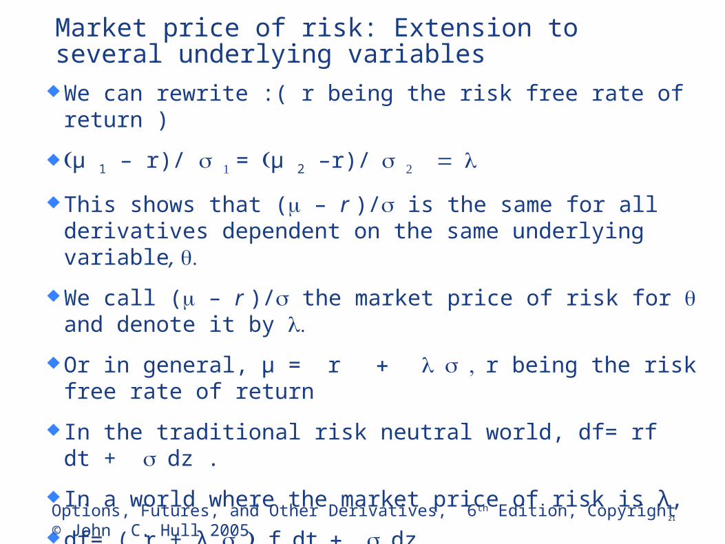
Market price of risk: Extension to several underlying variables¨ We can rewrite :( r being the risk free rate of return )

¨ (µ 1 – r)/ s 1 = (µ 2 –r)/ s 2 =

¨ This shows that (m – r )/s is the same for all derivatives dependent on the same underlying variable, .q

¨ We call (m – r )/s the market price of risk for q and denote it by .l

¨ Or in general, µ = r + , s r being the risk free rate of return

¨ In the traditional risk neutral world, df= rf dt + s dz .

¨ In a world where the market price of risk is λ,

¨ df= ( r + λ )s f dt + s dz

¨ In general, df/f = µdt + si dzi , µ - r = λi si 21

Options, Futures, and Other Derivatives, 6th Edition, Copyright © John C. Hull 2005

Estimating market price of risk

¨ According to Capital Asset Pricing Model,

¨ µ - r = ( / s m) [ µm - r] ( ( / s m) is also called )

¨ Where r is short term risk free rate, m denotes the market portfolio, is the correlation coefficient between asset and market returns

¨ But µ - r =

¨ Or = ( / m) [ µm - r]

22

Problem

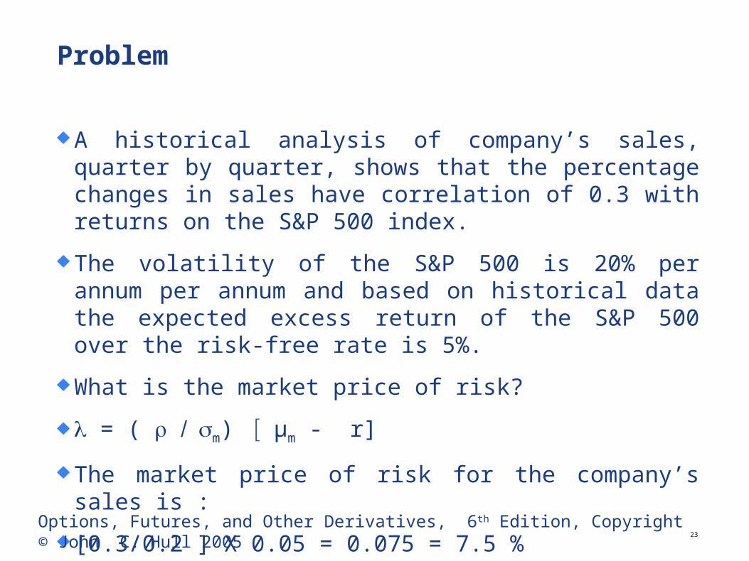
¨ A historical analysis of company’s sales, quarter by quarter, shows that the percentage changes in sales have correlation of 0.3 with returns on the S&P 500 index.

¨ The volatility of the S&P 500 is 20% per annum per annum and based on historical data the expected excess return of the S&P 500 over the risk-free rate is 5%.

¨ What is the market price of risk?

¨ = ( / m) [ µm - r]

¨ The market price of risk for the company’s sales is :

¨ [0.3/0.2 ] X 0.05 = 0.075 = 7.5 %

¨23

Options, Futures, and Other Derivatives, 6th Edition, Copyright © John C. Hull 2005

Problem¨ The market price of risk for copper is 0.5, the volatility of

copper prices is 20% per annum, the spot price is 80 cents per pound, and the 6-month futures price is 75 cents per pound. What is the expected percentage growth rate in copper prices over the next 6 months?

¨ In a risk-neutral world the expected price of copper in six months is 75 cents.

¨ This implies expected growth rate of 2ln(75/80) = - 12.9%/ year

¨ The increase in the growth rate when we move from the risk-neutral world to the real world is the volatility of copper times its market price of risk.

¨ This is 0.2 x 0.5 = 0.1 or 10% per annum.

¨ It follows that the expected growth rate of the price of copper in the real world is – 2.9%. 24Options, Futures, and Other Derivatives, 6th Edition, Copyright © John C.

Hull 2005

Problem

¨ The correlation between a company’s gross revenue and the market index is 0.2.

¨ The excess return of the market over the risk-free rate is 6% and the volatility of the market index is 18%.

¨ What is the market price of risk for the company’s revenue?

¨ = ( / m) [ µm - r]

¨ ρ = 0.2, µm – r =0.06, and σm =0.18.

¨ It follows that the market price of risk is

¨ [0.2 X 0.06] / 0.18 = 0.067

25Options, Futures, and Other Derivatives, 6th Edition, Copyright © John C. Hull 2005

A driver entering into a car lease agreement can obtain the right to buy a car in 4 years for $10,000. The current value of the car is $30,000. The value of the car, S, is expected to follow the process dS = µSdt + σSdz Iif µ = - 0.25, σ = 0.15, and dz is a Wiener Process. The market price of risk for the car price is estimated to be 0.1. What is the value of the option? Assume that the risk-free rate for all maturities is 6%.

¨ The expected growth rate of the car price in a risk-neutral world is --0.25 + (0.1 x 0.15) = -0.235.

¨ The expected value of the car in a risk-neutral world in four years, Ê(ST), is therefore 30,000e-0.235X4 =$11,719.

¨ Using the result in the appendix to the value of the option is e-rT [Ê(ST) N (d1) – KN(d2)]

¨ Where

¨ r = 0.06, σ = 0.15, T = 4, and K = 10,000.

¨ d1 = .6787, N (d1) = .7512, d2 = .3787, N(d2) = .6476

¨ C= [(11719)(.7512) – (10,000)(.6476)]e-.24 = $183026

T

TKd

2/)/)Ê(Sln( 2

T1

T

TKd

2/)/)Ê(Sln( 2

T2

Options, Futures, and Other Derivatives, 6th Edition, Copyright © John C. Hull 2005

Problem

¨ The cost of renting commercial real estate in a certain city is quoted as the amount that would be paid per square foot per year in a new 5-year rental agreement. The current cost is $30 per square foot. The expected growth rate of the cost is 12% per annum, its volatility is 20% per annum, and its market price of risk is 0.3. A company has the opportunity to pay $1 million now for the option to rent 100,000 square feet at $35 per square foot for a 5-year period starting in 2 years. The risk-free rate is 5% per annum (assumed constant). Is this option worth buying?

27

John C Hull, Options, Futures and Other Derivatives

Solution¨ Define V as the quoted cost per square foot of office space in 2

years. Assume the rent is paid annually in advance. Payoff from the option is

¨ 100,000 A max (V – 35, 0)

¨ A = 1 + 1 x e-0.05x1 + 1 x e-0.05x2 + 1 x e-0.05x3 + 1 x e-0.05x4 = 4.5355

¨ The expected payoff in a risk-neutral world is there

¨ 100,000 x 4.5355 x Ê[max (V – 35, 0)] = 453,550 x Ê[ max(V – 35, 0)]

¨ where Ê denotes expectations in a risk-neutral world. Using the result in equation (13A.1), this is

¨ Value of option = 453,550[Ê(V)N(d1) – 35N(d2)]

28

Cont… ¨ where

¨ The expected growth rate in the cost of commercial real estate in a risk-neutral world is r = m – λs where m is real world growth rate, s is volatility, λ is market price of risk.

¨ Here m = 0.12, s = 0.2, and λ = 0.3, so that the expected risk-neutral growth rate is 0.06, or 6% per year.

¨ E(V) = 30e0.06x2 = 33.82. d1 =0.0202 , N(d1) = 0.5088

¨ d2 =-0.2627, N(d2)=0.3966

¨ C =$ ( 453,550) [(33.82)(.5088) – (.35)(.3966)] = $ 1.5015 million.

¨ Discounting at the risk-free rate the value of the option is 1.5015e-0.05x2 = $1.3586 million.

¨ This shows that it is worth paying $1 million for the option.29

22.0

2/22.Ê(V)/35ln 2

1

d

22.0

2/22.Ê(V)/35ln 2

2

d