Real-Estate Agent Commission Structure and Sales

Performance

Pieter Gautier∗ Arjen Siegmann† Aico van Vuuren‡

This version: February 2017

Abstract

Do higher real-estate agent fees imply better performance? This study uses a

nation-wide dataset of residential real-estate transactions in the Netherlands

from 1985 to 2011 to provide evidence against this. Brokers with a flat-fee

structure who charge a relatively low up-front fee and leave the viewings to

the seller sell at least as fast and at – on average – 2.7 percent higher prices.

We correct for fixed house- and time effects and our results are robust to using

a variety of different specifications.

Keywords: real-estate brokers, rent seeking, housing market

JEL-Classification: D8, L1, L8, R2, R3

∗Vrije Universiteit Amsterdam.†Vrije Universiteit Amsterdam, Corresponding author, a.h.siegmannvu.nl.‡University of Gothenburg.

The authors thank Johan Walden, seminar participants at the VU and the European Finance As-sociation 2016 for useful comments and suggestions. We thank NVM, the “Nederlandse Verenigingvan Makelaars o.g. en vastgoeddeskundigen” for providing the data.

1 Introduction

The majority of residential home sales is realized through the help of a real-estate

agent.1 This is not surprising because both buying and selling a home involve

decisions that can have a large and long-lasting financial impact, and consumers

are typically not well informed about the real-estate market. However, real-estate

agents are expensive: a typical real-estate agent who represents the seller charges 6

percent of the sales price in the US, while the fee is between 2 and 3 percent in the

UK and about 2 percent in the Netherlands.2 According to White (2007), 61 billion

dollars were spent on real-estate transaction fees in 2004 in the US.3 Whether or

not those fees are excessive is an empirical question that we address in this paper.

If real-estate agents are very good in bringing (heterogeneous) sellers and buyers

together, they create surplus that could in principle justify high fees. So in order to

create surplus, real-estate agents should sell faster and/or at a higher price.

This paper addresses the performance of real-estate agents using a unique

case study for the Netherlands. In contrast to the US, almost all of the residential

property for sale is listed publicly in the Netherlands (as of 2001) on an internet

site called Funda. Originally, only traditional full-service brokers posted the houses

of their clients on this website and charged a fee of around 2 percent, payable after

the transaction was made (the average transaction price was almost 200,000 Euro).

In 2005, flat-fee brokers entered the market. These brokers charge an up-front fee,

1According to realtor.org, 89 percent of home sellers in the United States use a real-estate agent,while this number is 87 percent for home buyers.

2Note that in the US, the 6 percent also includes the fee that the real-estate agent of the sellerneeds to pay to the real-estate agent of the buyer.

3Based on the data provided on realtor.org, we obtain a figure of 70 billion dollars for 2015. Thisconjecture is fed by the fact that most countries have a brokerage fee which is a fixed percentageof the sales price. See OECD (2007) for a complete list of brokerage fees.

1

in the range of 400 to 1300 Euro, which is only a fraction of the average fee of the

traditional brokers. In addition to charging a flat fee, these brokers use the same

online multiple listing service as the traditional brokers. Moreover, they offer limited

additional services, such as price negotiation. The main difference with traditional

brokers is that they leave the viewings of the house to the seller.

We find the flat-fee strategy to be the only broker characteristic that is sig-

nificant in explaining differences in transaction prices and time to sell. Other broker

properties such as proximity, experience and size have no significant effect on these

outcomes. Houses sold through a flat-fee broker obtain a 2.7 percent higher price

and sell significantly faster. The difference in transaction prices is almost unrespon-

sive to alternative specifications, such as conditioning on high- and low prices, the

type of house and the density of houses for sale in the same neighborhood. We

also do not find that homeowners who switch from a flat-fee broker to a traditional

broker obtain a significantly higher price than those who started with a traditional

broker. This rules out simple explanations such as differences in price or liquidity

of the house or selection of unobservable house characteristics.

Our paper is related to Hendel et al. (2009), who look at the difference in price

and time on the market between the realtors’ MLS and a for-sale-by-owner (FSBO)

website in Madison. Given that all of our transactions take place on the same

platform, we are able to single out the impact of the additional services provided by

the traditional real-estate agents rather than a combination of services and quality

of the platform. Hendel et al. (2009) find that houses that are originally listed on an

FSBO website sell at a higher price no matter whether those houses are sold through

the realtors’ MLS or through the FSBO website, while we find that traditional real-

estate agents who receive a percentage of the selling price sell at a lower price than

2

the flat-fee agents.

Our paper is also related to Bernheim and Meer (2013), who look at houses

sold at the university campus of Stanford. Similar to the paper of Hendel et al.

(2009), they compare FSBO sales with brokered sales. However, in contrast to

Hendel et al. (2009), but in line with our research, the Stanford study listed all

campus sales on one single open-access listing service, which is available regardless

of whether a broker is used or not. One caveat of the paper of Bernheim and

Meer (2013) is that the number of observations is low and the Stanford housing

market may not be representative for the total population because homeownership

at the campus is limited to Stanford faculty and some senior staff. Nevertheless, an

advantage of their analysis is that the sellers are a relatively homogeneous group,

which reduces the risk of seller selection into FSBO sales. Our group of sellers is

more heterogeneous, but also in our study the risk of seller selection is small because

sellers that use flat-fee brokers only perform a relatively simple task: providing the

viewings of the house. Therefore, differences in negotiation skills between buyers

and the potential stigma of FSBO sales cannot explain our results.

We also contribute to the literature on potential agency problems for dele-

gated brokers in real estate (see Rutherford and Yavas, 2012, Han and Hong, 2011,

Bergstresser et al. 2009, and Del Guercio et al. ,2010). Our result of a 2.7 percent

difference in transaction performance is substantial – and obviously larger than the

opportunity costs of the time spent when someone decides to sell the house through

a low-service flat-fee broker. The result for flat-fee brokers is similar in size to that of

brokers who sell a house that they own themselves; see Rutherford et al. (2005) and

Levitt and Syverson (2008b). The higher price obtained by a broker-owner can be

explained by the superior information available to the broker and the higher effort

3

level he or she expands. Finally, our results are relevant for the literature on the role

of platforms in intermediation; see Hendel et al. (2009). Our results suggest that

once houses are listed on a platform, a simple structure of a flat fee and minimal

additional services performs very well in terms of a high transaction price and fast

sale.

We find no evidence that brokers with offices located in the proximity of the

seller perform better. This contrasts with earlier studies on the relation between

geographical proximity and investor performance by stock investors, hedge funds,

investors in municipal bonds and investors in mutual funds; see Teo (2009) and

Butler (2008). Ivkovic and Weisbenner (2005) find that households have a strong

preference for stocks that are geographically close. Moreover, they find that local

investors seem to have some degree of superior information.

The rest of this paper is organized as follows. Section 2 describes the insti-

tutional aspects of real-estate brokerage in the Netherlands. Section 3 describes the

data. Section 4 describes the empirical approach and estimates. Section 5 provides

additional robustness analyses. Section 6 discusses some potential explanations for

our main results. Section 7 concludes.

2 Real-estate agents in the Netherlands

In the Netherlands, real-estate agents can work independently, but most are mem-

bers of a real-estate association. The largest association is the National Association

of Real-Estate Brokers and Real-Estate Valuers (NVM), to which seventy percent

of all real-estate agents belong. In terms of transactions, NVM had a 75 percent

market share measured over 2010 and 2011.

4

In January 2001, NVM launched a website, funda.nl, where all the houses of

its members are listed. Funda quickly became the dominant platform for potential

buyers, as it eliminated the need for a buy-side broker and made all the houses

and their details visible for free. In 2010, Funda started to list houses of non-NVM

agents as well.

Before 1999, NVM had a recommended fee of around 2 percent of the sales

price.4 The recommended fee was abolished in 1999, under the threat of sanctions

from the anti-trust authority. Still, although the fees have been decreasing in terms

of the percentage of the sales price, anecdotal evidence suggests that many agents

continue to use fees close to 2 percent. In addition, brokers are reluctant to negotiate

the fee and, with the exception of the flat-fee brokers, they do not openly compete

on price.

Starting in 2005, flat-fee brokers entered the market as members of the bro-

kers association. They charge an up-front, fixed fee. At the moment of our research,

the fee of these brokers was in the range of 400 to 1300 Euro. In return, they list

a house on Funda, advise on the list price and perform the negotiation. The major

difference with a traditional broker is that the viewing of the house is scheduled and

hosted by the seller.

In response to the Funda platform, some so-called for-sale-by-owner websites

have sprung up where sellers list their house directly, without the intermediation

of a broker. However, in contrast to other countries (such as the US), this has not

caught on in a significant way (Hendel et al., 2009, and Bernheim and Meer, 2013).

4The recommended fee was 1.85 percent excluding VAT.

5

3 Data

The dataset of transaction prices, obtained from the NVM, contains the properties

of houses and apartments sold between 1985 and 2011, as well as a unique identifier

for the real-estate agent. The dataset does not contain objects that are rented out.

Note that the use of this dataset implies that we do not observe transactions that

are not represented by a broker that is a member of the association. Nevertheless,

the benefit of using this dataset is that all of our transactions since 2001 were listed

on the Funda website, which guarantees the use of one and the same platform for

every house sale in our dataset.

Starting from 2,007,914 transactions, we remove observations with missing

house size (in square meters) and missing lot size (if not an apartment). Then, the

following filters are applied: we discard observations with a list price or transaction

price below ten thousand Euro and above one hundred million Euro, an absolute

percentage change in transaction price relative to list price of more than fifty percent,

a size of less than twenty square meters, and selling date equal to or before list date.

Also, we discard observations with other obvious errors. Furthermore, we remove

observations with brokers for which we were unable to find their associated profile

(see below) and transactions on houses that have not sold since 2005 (i.e., the

year in which flat-fee commission brokers became active).5 We also delete 327,097

transactions that represented a house that is only sold once in our dataset and

therefore drops out of our analysis since we use house fixed effects in all of our

regression equations of Section 4. This leaves us with 380,252 observations which are

5We cannot remove all observations prior to 2005, as we need them to allow for house fixedeffects.

6

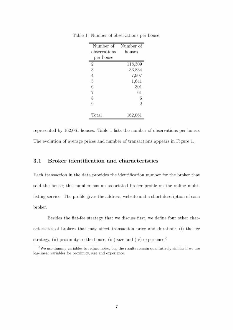
Table 1: Number of observations per house

Number of Number ofobservations houses

per house

2 118,3093 33,8344 7,9075 1,6416 3017 618 69 2

Total 162,061

represented by 162,061 houses. Table 1 lists the number of observations per house.

The evolution of average prices and number of transactions appears in Figure 1.

3.1 Broker identification and characteristics

Each transaction in the data provides the identification number for the broker that

sold the house; this number has an associated broker profile on the online multi-

listing service. The profile gives the address, website and a short description of each

broker.

Besides the flat-fee strategy that we discuss first, we define four other char-

acteristics of brokers that may affect transaction price and duration: (i) the fee

strategy, (ii) proximity to the house, (iii) size and (iv) experience.6

6We use dummy variables to reduce noise, but the results remain qualitatively similar if we uselog-linear variables for proximity, size and experience.

7

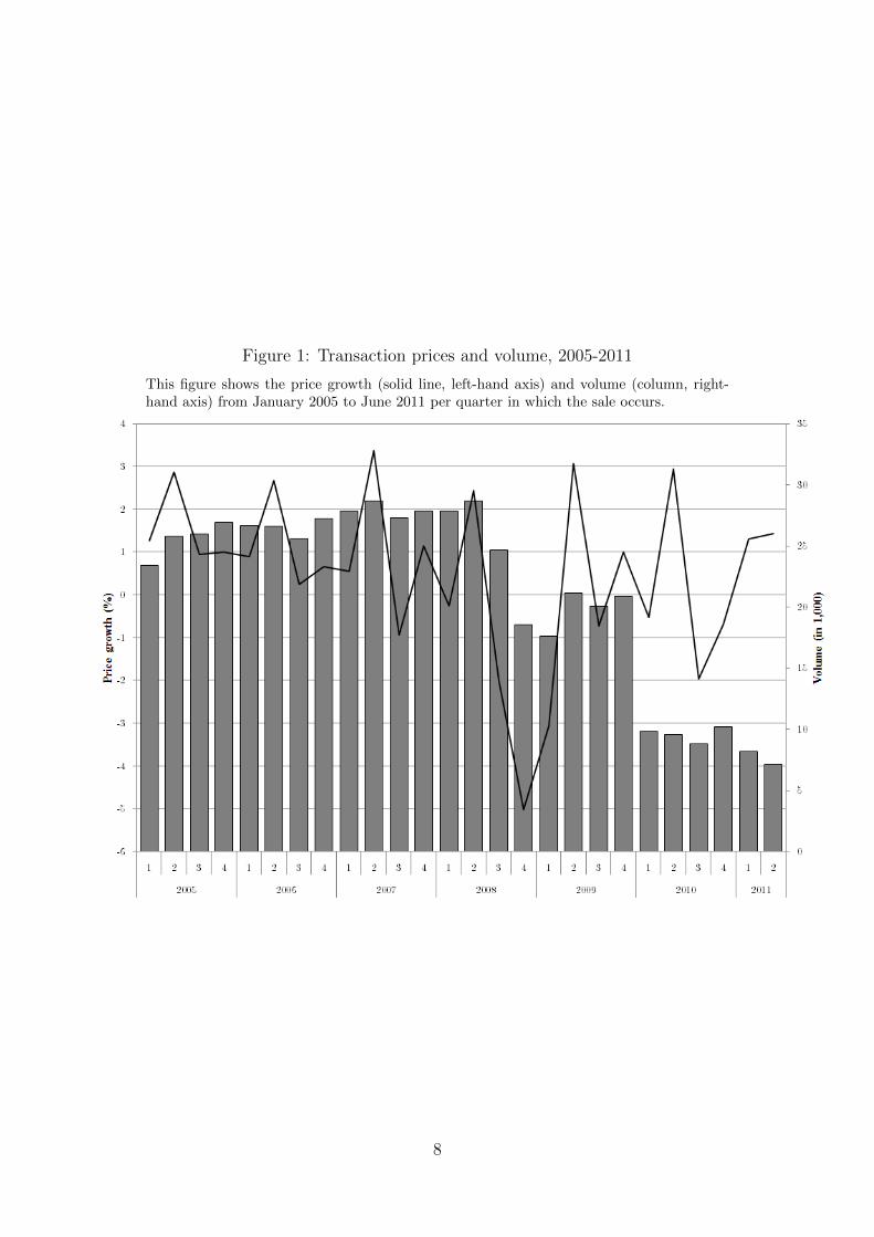
Figure 1: Transaction prices and volume, 2005-2011

This figure shows the price growth (solid line, left-hand axis) and volume (column, right-hand axis) from January 2005 to June 2011 per quarter in which the sale occurs.

8

3.2 Fee strategy

The listing platform has a separate section that lists brokers. We use the search

phrase ”flat fee” to find the brokers who advertise with a flat-fee structure and

identify a total of thirteen brokers with a total market share of 2.3 percent of all

transactions since 2005 (i.e., the year in which they first became active). The brokers

are active throughout the country and this is reflected in the transactions (i.e., flat-

fee transactions are not limited to one or a few specific regions).

3.3 Proximity

To find the geographical location of the broker, we take the address on the broker’s

profile page and feed it into a geocoding service in order to obtain the x and y

spatial coordinates. The geocoding was done in 2011 and 2012 to minimize the

measurement errors from relocations of real-estate agents. We compute the absolute

distance between each object and its broker using the x and y spatial coordinates.

The dummy variable ‘Close-by’ is 1 if the house is within the smallest 20th percentile

of distances between houses and brokers, which is approximately 800 meters.

3.4 Size

We compute the number of transactions per broker, per year, and determine large

brokers as those with a size above the 80th percentile.

3.5 Experience

We define the experience of a broker as the difference between the current year and

the first year that a broker has sold a house. The dummy variable ‘Experienced’ is

9

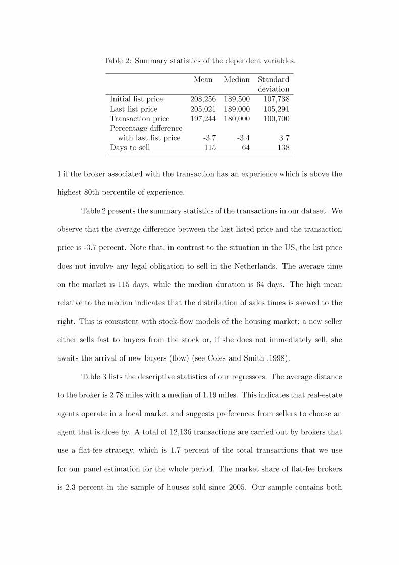
Table 2: Summary statistics of the dependent variables.

Mean Median Standarddeviation

Initial list price 208,256 189,500 107,738Last list price 205,021 189,000 105,291Transaction price 197,244 180,000 100,700Percentage difference

with last list price -3.7 -3.4 3.7Days to sell 115 64 138

1 if the broker associated with the transaction has an experience which is above the

highest 80th percentile of experience.

Table 2 presents the summary statistics of the transactions in our dataset. We

observe that the average difference between the last listed price and the transaction

price is -3.7 percent. Note that, in contrast to the situation in the US, the list price

does not involve any legal obligation to sell in the Netherlands. The average time

on the market is 115 days, while the median duration is 64 days. The high mean

relative to the median indicates that the distribution of sales times is skewed to the

right. This is consistent with stock-flow models of the housing market; a new seller

either sells fast to buyers from the stock or, if she does not immediately sell, she

awaits the arrival of new buyers (flow) (see Coles and Smith ,1998).

Table 3 lists the descriptive statistics of our regressors. The average distance

to the broker is 2.78 miles with a median of 1.19 miles. This indicates that real-estate

agents operate in a local market and suggests preferences from sellers to choose an

agent that is close by. A total of 12,136 transactions are carried out by brokers that

use a flat-fee strategy, which is 1.7 percent of the total transactions that we use

for our panel estimation for the whole period. The market share of flat-fee brokers

is 2.3 percent in the sample of houses sold since 2005. Our sample contains both

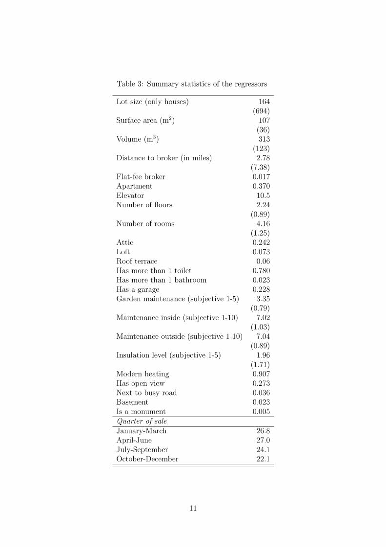
Table 3: Summary statistics of the regressors

Lot size (only houses) 164(694)

Surface area (m2) 107(36)

Volume (m3) 313(123)

Distance to broker (in miles) 2.78(7.38)

Flat-fee broker 0.017Apartment 0.370Elevator 10.5Number of floors 2.24

(0.89)Number of rooms 4.16

(1.25)Attic 0.242Loft 0.073Roof terrace 0.06Has more than 1 toilet 0.780Has more than 1 bathroom 0.023Has a garage 0.228Garden maintenance (subjective 1-5) 3.35

(0.79)Maintenance inside (subjective 1-10) 7.02

(1.03)Maintenance outside (subjective 1-10) 7.04

(0.89)Insulation level (subjective 1-5) 1.96

(1.71)Modern heating 0.907Has open view 0.273Next to busy road 0.036Basement 0.023Is a monument 0.005Quarter of saleJanuary-March 26.8April-June 27.0July-September 24.1October-December 22.1

11

multi-floor houses and apartments. A seasonal effect is visible in the lower number

of houses sold in the fourth quarter (22 percent) relative to the first (27 percent).

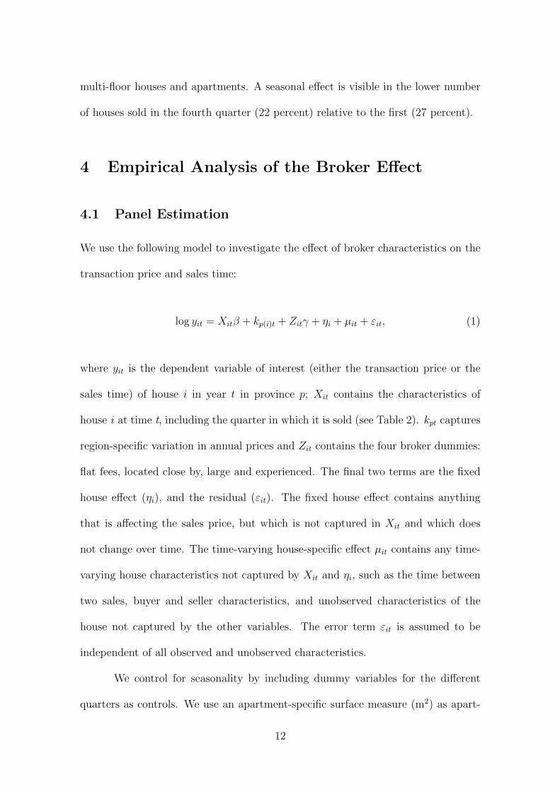
4 Empirical Analysis of the Broker Effect

4.1 Panel Estimation

We use the following model to investigate the effect of broker characteristics on the

transaction price and sales time:

log yit = Xitβ + kp(i)t + Zitγ + ηi + µit + εit, (1)

where yit is the dependent variable of interest (either the transaction price or the

sales time) of house i in year t in province p; Xit contains the characteristics of

house i at time t, including the quarter in which it is sold (see Table 2). kpt captures

region-specific variation in annual prices and Zit contains the four broker dummies:

flat fees, located close by, large and experienced. The final two terms are the fixed

house effect (ηi), and the residual (εit). The fixed house effect contains anything

that is affecting the sales price, but which is not captured in Xit and which does

not change over time. The time-varying house-specific effect µit contains any time-

varying house characteristics not captured by Xit and ηi, such as the time between

two sales, buyer and seller characteristics, and unobserved characteristics of the

house not captured by the other variables. The error term εit is assumed to be

independent of all observed and unobserved characteristics.

We control for seasonality by including dummy variables for the different

quarters as controls. We use an apartment-specific surface measure (m2) as apart-

12

ments lack some characteristics that houses have, such as the lot size and garden,

which might influence the shadow price of surface for apartments. As the time

between consecutive sales might affect pricing, we also include a variable that mea-

sures the time in years since the previous sale of the house. All quantity variables in

Xit are in logs. We use twenty-two regional dummy variables for the construction of

kp(i)t in (1): ten for the largest cities and twelve for the provinces in the Netherlands.

The error term, ηit, is assumed to be independent and identically distributed.

The model in (1) is similar to that of Levitt and Syverson (2008b) and Rutherford

et al. (2005), except that we have the broker variables as additional explanatory

variables.

The parameters in equation (1) can be estimated using fixed effects under

the condition that time-varying house-specific effects are absent or that they are

not correlated with any of the observed characteristics, including the seller’s choice

to use a flat-fee real-estate broker. This is also the strategy used, for example, in

Hendel et al. (2009).

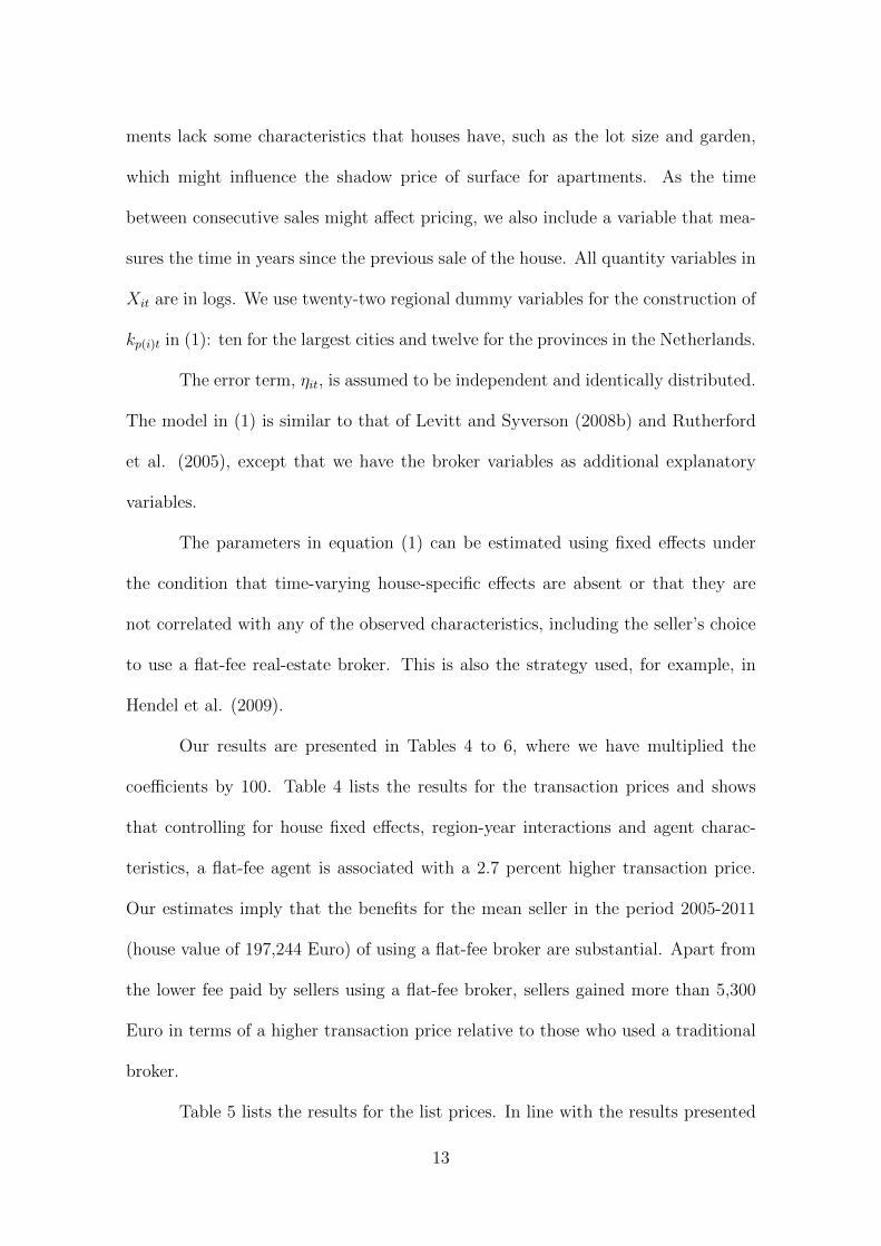
Our results are presented in Tables 4 to 6, where we have multiplied the

coefficients by 100. Table 4 lists the results for the transaction prices and shows

that controlling for house fixed effects, region-year interactions and agent charac-

teristics, a flat-fee agent is associated with a 2.7 percent higher transaction price.

Our estimates imply that the benefits for the mean seller in the period 2005-2011

(house value of 197,244 Euro) of using a flat-fee broker are substantial. Apart from

the lower fee paid by sellers using a flat-fee broker, sellers gained more than 5,300

Euro in terms of a higher transaction price relative to those who used a traditional

broker.

Table 5 lists the results for the list prices. In line with the results presented

13

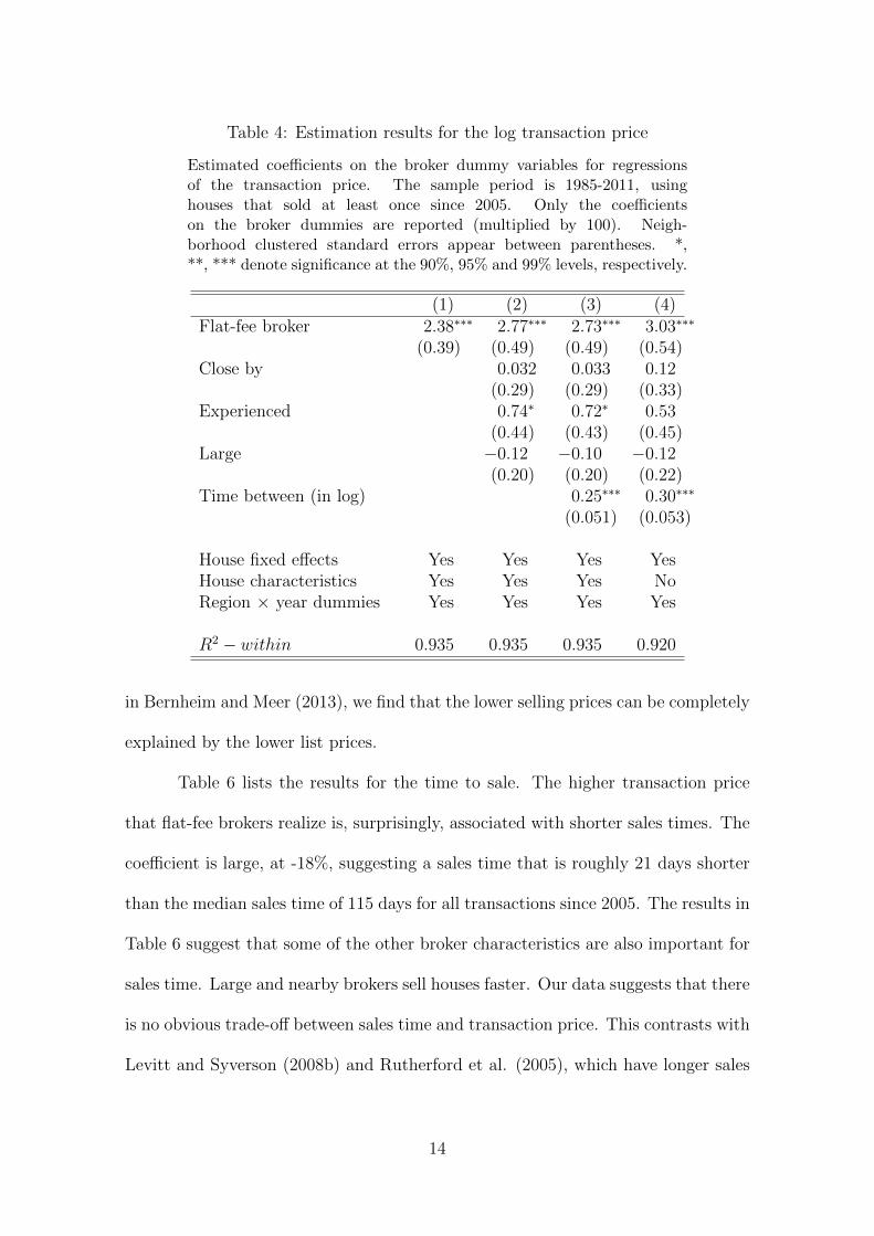
Table 4: Estimation results for the log transaction price

Estimated coefficients on the broker dummy variables for regressionsof the transaction price. The sample period is 1985-2011, usinghouses that sold at least once since 2005. Only the coefficientson the broker dummies are reported (multiplied by 100). Neigh-borhood clustered standard errors appear between parentheses. *,**, *** denote significance at the 90%, 95% and 99% levels, respectively.

(1) (2) (3) (4)Flat-fee broker 2.38∗∗∗ 2.77∗∗∗ 2.73∗∗∗ 3.03∗∗∗

(0.39) (0.49) (0.49) (0.54)Close by 0.032 0.033 0.12

(0.29) (0.29) (0.33)Experienced 0.74∗ 0.72∗ 0.53

(0.44) (0.43) (0.45)Large −0.12 −0.10 −0.12

(0.20) (0.20) (0.22)Time between (in log) 0.25∗∗∗ 0.30∗∗∗

(0.051) (0.053)

House fixed effects Yes Yes Yes YesHouse characteristics Yes Yes Yes NoRegion × year dummies Yes Yes Yes Yes

R2 − within 0.935 0.935 0.935 0.920

in Bernheim and Meer (2013), we find that the lower selling prices can be completely

explained by the lower list prices.

Table 6 lists the results for the time to sale. The higher transaction price

that flat-fee brokers realize is, surprisingly, associated with shorter sales times. The

coefficient is large, at -18%, suggesting a sales time that is roughly 21 days shorter

than the median sales time of 115 days for all transactions since 2005. The results in

Table 6 suggest that some of the other broker characteristics are also important for

sales time. Large and nearby brokers sell houses faster. Our data suggests that there

is no obvious trade-off between sales time and transaction price. This contrasts with

Levitt and Syverson (2008b) and Rutherford et al. (2005), which have longer sales

14

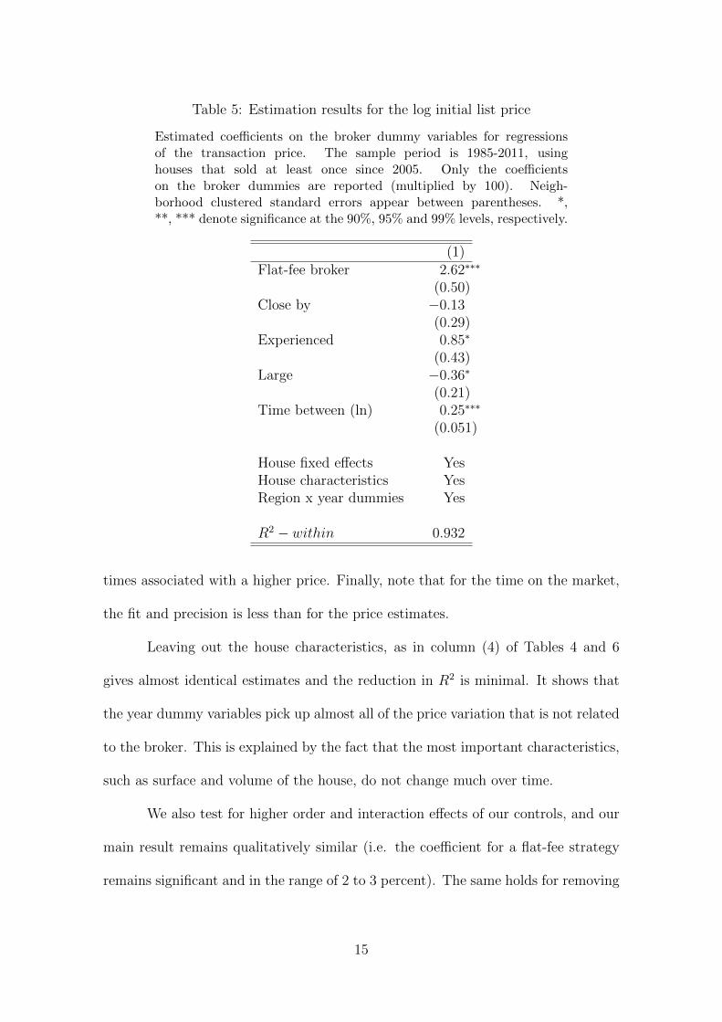
Table 5: Estimation results for the log initial list price

Estimated coefficients on the broker dummy variables for regressionsof the transaction price. The sample period is 1985-2011, usinghouses that sold at least once since 2005. Only the coefficientson the broker dummies are reported (multiplied by 100). Neigh-borhood clustered standard errors appear between parentheses. *,**, *** denote significance at the 90%, 95% and 99% levels, respectively.

(1)Flat-fee broker 2.62∗∗∗

(0.50)Close by −0.13

(0.29)Experienced 0.85∗

(0.43)Large −0.36∗

(0.21)Time between (ln) 0.25∗∗∗

(0.051)

House fixed effects YesHouse characteristics YesRegion x year dummies Yes

R2 − within 0.932

times associated with a higher price. Finally, note that for the time on the market,

the fit and precision is less than for the price estimates.

Leaving out the house characteristics, as in column (4) of Tables 4 and 6

gives almost identical estimates and the reduction in R2 is minimal. It shows that

the year dummy variables pick up almost all of the price variation that is not related

to the broker. This is explained by the fact that the most important characteristics,

such as surface and volume of the house, do not change much over time.

We also test for higher order and interaction effects of our controls, and our

main result remains qualitatively similar (i.e. the coefficient for a flat-fee strategy

remains significant and in the range of 2 to 3 percent). The same holds for removing

15

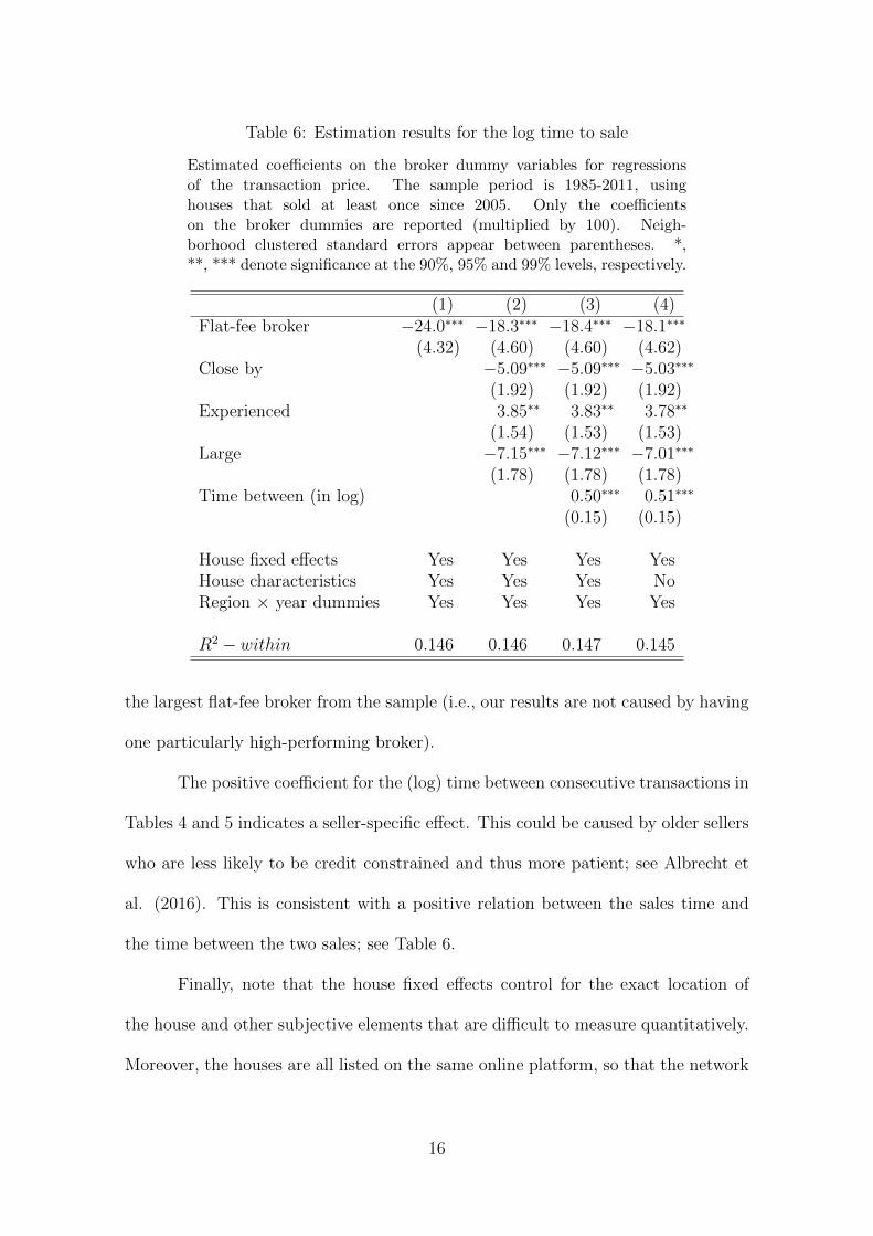
Table 6: Estimation results for the log time to sale

Estimated coefficients on the broker dummy variables for regressionsof the transaction price. The sample period is 1985-2011, usinghouses that sold at least once since 2005. Only the coefficientson the broker dummies are reported (multiplied by 100). Neigh-borhood clustered standard errors appear between parentheses. *,**, *** denote significance at the 90%, 95% and 99% levels, respectively.

(1) (2) (3) (4)Flat-fee broker −24.0∗∗∗ −18.3∗∗∗ −18.4∗∗∗ −18.1∗∗∗

(4.32) (4.60) (4.60) (4.62)Close by −5.09∗∗∗ −5.09∗∗∗ −5.03∗∗∗

(1.92) (1.92) (1.92)Experienced 3.85∗∗ 3.83∗∗ 3.78∗∗

(1.54) (1.53) (1.53)Large −7.15∗∗∗ −7.12∗∗∗ −7.01∗∗∗

(1.78) (1.78) (1.78)Time between (in log) 0.50∗∗∗ 0.51∗∗∗

(0.15) (0.15)

House fixed effects Yes Yes Yes YesHouse characteristics Yes Yes Yes NoRegion × year dummies Yes Yes Yes Yes

R2 − within 0.146 0.146 0.147 0.145

the largest flat-fee broker from the sample (i.e., our results are not caused by having

one particularly high-performing broker).

The positive coefficient for the (log) time between consecutive transactions in

Tables 4 and 5 indicates a seller-specific effect. This could be caused by older sellers

who are less likely to be credit constrained and thus more patient; see Albrecht et

al. (2016). This is consistent with a positive relation between the sales time and

the time between the two sales; see Table 6.

Finally, note that the house fixed effects control for the exact location of

the house and other subjective elements that are difficult to measure quantitatively.

Moreover, the houses are all listed on the same online platform, so that the network

16

effects of different platforms or sellers are not driving our results. Thus, our results

reported in Tables 4 to 6 cannot be explained by an information effect: the sellers

involved in these transactions have exactly the same information.

5 Robustness

5.1 Interaction effects

The hedonic model in (1) might be misspecified with regard to nonlinear relations

between house characteristics and (log) prices. We can control for this by introducing

interactions of variables of interest with the flat-fee dummy.

The first interaction concerns price. Expensive houses might be underpriced

in the log-linear hedonic model and sold more often by a flat fee. In that case, the

coefficient in the full sample might be driven by a limited number of expensive houses

with a successful house sale using a broker with a flat-fee strategy. Also, given that

a traditional fee is a percentage of the transaction price, the monetary incentives to

choose a broker that uses a flat-fee strategy are higher for more expensive houses. In

order to investigate this, we interact an above-median price dummy with the flat-fee

broker dummy.

A second concern is that apartments and houses in high-density areas could

be overrepresented in the sample of houses that are sold through the use of a flat-fee

broker. Apartments are easier to price, since they have fewer unique characteristics,

making it possible to find almost identical objects (such as apartments in the same

building that have been sold before). Likewise, sellers in neighborhoods with a high-

density of houses might find it easier to set a list price based on comparable objects

17

and be more inclined to choose a flat-fee broker. We control for these effects by

interacting the flat-fee dummy with the dummy variable for apartments and the

dummy variable for above-median neighborhood densities.

A third concern is that sophisticated sellers are more likely to sell using

a cheaper flat-fee real-estate agent. We expect that this selection effect would be

largest in the earliest years of the introduction of flat-fee real-estate agents, since the

most sophisticated sellers are also the ones who are most likely to be early adopters

of the new selling strategy. Moreover, the number of sales made with flat-fee real-

estate agents has been increasing over time, which immediately implies a decrease

in the selectivity of the sophisticated sellers. This hypothesis implies that we should

expect a declining impact of flat-fee brokers since their introduction in 2005. We

test this by interacting the flat-fee dummy with a dummy that is 1 in the years prior

to 2008.

A fourth issue is that traditional real-estate agents could be exerting more

effort in the fourth quarter in order to meet their annual sales target. This effect is

absent under a flat fee, where fees are earned up-front. We therefore interact our

flat-fee dummy with a dummy for the fourth quarter.

A final concern is that the distribution of sales times could be more fat-tailed

for those sales involving the help of a flat-fee broker. That is, traditional brokers

would be more effective for difficult-to-sell houses, while a flat-fee structure would

be better for liquid properties. To test this, we interact with a dummy variable

that is 1 if the sales time is higher than the median. Note that the interpretation

of this variable is complicated by the fact that sales time is endogenous. That is,

unobserved characteristics that affect the sales time also affect the selling price of

the house. Nevertheless, due to the expected negative relationship between the two

18

outcome variables, the absolute value of the coefficient estimates can be interpreted

as an upper bound of the real effect.

Table 7 reports the estimation results for transaction prices with interaction

effects. The conclusion that can be drawn from this Table is that in all alternative

specifications, the positive flat-fee effect remains. The only statistically significant

terms are the ones with sales time and the fourth quarter dummy. The sales-time

effect is such that flat-fee houses sell 4.1 percent faster. For longer sales times, the

performance is reduced to 1.3 percent, but as stated in the previous paragraph, this

can be interpreted as a lower bound. If anything, this indicates that even houses

with a long time to sale obtain a higher price when using a flat-fee broker. The

fourth-quarter effect suggests that traditional brokers put more effort into selling a

house in the fourth quarter, reducing the performance gap with fixed-fee brokers to

1.5 percent (3.07 - 1.64). This supports an end-of-year effect on the part of real-

estate agents aiming to reach a sales target. Such effects exist in many industries

where compensation schemes depend on yearly sales in a non-linear way; see Oyer

(1998). To summarize, the evidence points to a sizable and significantly positive

effect associated with a flat fee on the part of the seller that is not explained by

interactions with other variables.

5.2 Sellers switching agents

As in the analysis of Hendel et al. (2009), another way to investigate the selection

effect of sellers is to look at the sellers who initially started with one type of broker

(for example, a flat-fee broker) and then switched to another type (say, a traditional

broker), for the same property. If the switching between brokers is random, then

19

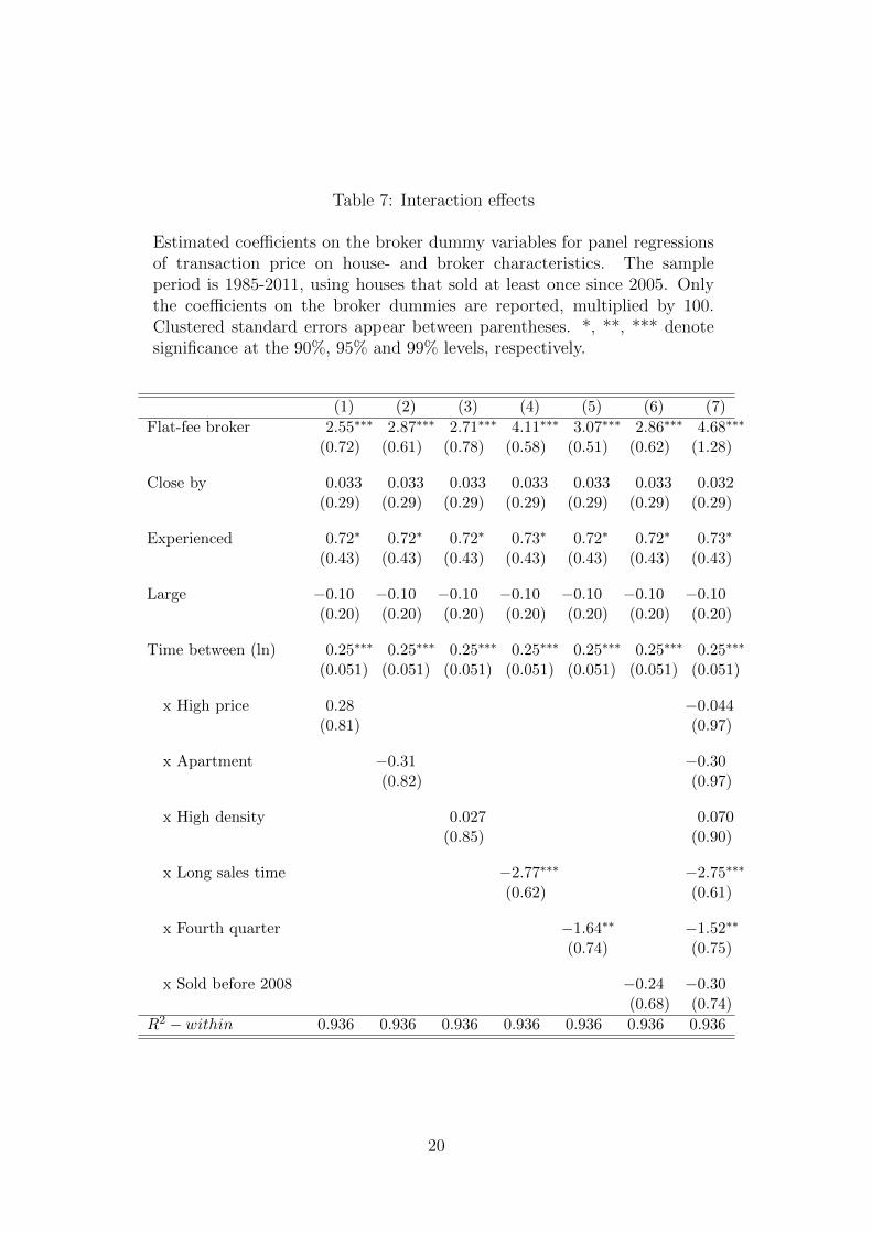
Table 7: Interaction effects

Estimated coefficients on the broker dummy variables for panel regressionsof transaction price on house- and broker characteristics. The sampleperiod is 1985-2011, using houses that sold at least once since 2005. Onlythe coefficients on the broker dummies are reported, multiplied by 100.Clustered standard errors appear between parentheses. *, **, *** denotesignificance at the 90%, 95% and 99% levels, respectively.

(1) (2) (3) (4) (5) (6) (7)

Flat-fee broker 2.55∗∗∗ 2.87∗∗∗ 2.71∗∗∗ 4.11∗∗∗ 3.07∗∗∗ 2.86∗∗∗ 4.68∗∗∗

(0.72) (0.61) (0.78) (0.58) (0.51) (0.62) (1.28)

Close by 0.033 0.033 0.033 0.033 0.033 0.033 0.032(0.29) (0.29) (0.29) (0.29) (0.29) (0.29) (0.29)

Experienced 0.72∗ 0.72∗ 0.72∗ 0.73∗ 0.72∗ 0.72∗ 0.73∗

(0.43) (0.43) (0.43) (0.43) (0.43) (0.43) (0.43)

Large −0.10 −0.10 −0.10 −0.10 −0.10 −0.10 −0.10(0.20) (0.20) (0.20) (0.20) (0.20) (0.20) (0.20)

Time between (ln) 0.25∗∗∗ 0.25∗∗∗ 0.25∗∗∗ 0.25∗∗∗ 0.25∗∗∗ 0.25∗∗∗ 0.25∗∗∗

(0.051) (0.051) (0.051) (0.051) (0.051) (0.051) (0.051)

x High price 0.28 −0.044(0.81) (0.97)

x Apartment −0.31 −0.30(0.82) (0.97)

x High density 0.027 0.070(0.85) (0.90)

x Long sales time −2.77∗∗∗ −2.75∗∗∗

(0.62) (0.61)

x Fourth quarter −1.64∗∗ −1.52∗∗

(0.74) (0.75)

x Sold before 2008 −0.24 −0.30(0.68) (0.74)

R2 − within 0.936 0.936 0.936 0.936 0.936 0.936 0.936

20

we are able to eliminate the selection effects by comparing those house sales that

involved a switch between broker types and the ones that did not. In order to inves-

tigate this, we employ an additional dataset that is obtained from screen-scraping

the listing site where all houses are advertised. The data were collected in the period

2004-2010; an earlier version of the dataset was used in Gautier et al. (2009).

We use the identification number of the first real-estate agent listing the

house online, and indicate a sale as a “switch” when this agent is different from the

agent at the time of sale. We find 3,680 transactions where the agent changed from

a flat-fee type to a traditional broker, and 80 transactions where the agent changed

from the traditional type to one with a flat fee.

The low number of switchers from traditional agents may be related to the

difference in switching costs: traditional agents usually charge a termination fee as

a compensation for the loss of income caused by the cancellation of the contract.

The opposite occurs for sellers with a flat-fee agent: since they have already paid

the fee up-front, their costs are sunk and hence there are no further monetary costs

involved in changing to another agent. The low number of switchers from traditional

to flat-fee is in line with Hendel et al. (2009), who also find a very low number of

switches from sellers represented by a real-estate broker using the MLS and sellers

who sell their own houses.

We create two additional dummy variables for the transactions: one for a

transaction that started with a traditional agent and ended with a flat-fee agent, and

one for a transaction that started with a flat-fee agent and ended with a traditional

agent.

The flat-fee effect is not changed, and there is only a significant effect for

sellers who come to a flat-fee agent in terms of the time to sale. This is in sharp

21

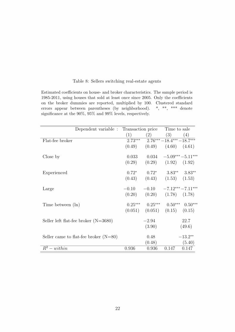
Table 8: Sellers switching real-estate agents

Estimated coefficients on house- and broker characteristics. The sample period is1985-2011, using houses that sold at least once since 2005. Only the coefficientson the broker dummies are reported, multiplied by 100. Clustered standarderrors appear between parentheses (by neighborhood). *, **, *** denotesignificance at the 90%, 95% and 99% levels, respectively.

Dependent variable : Transaction price Time to sale(1) (2) (3) (4)

Flat-fee broker 2.73∗∗∗ 2.76∗∗∗−18.4∗∗∗−18.7∗∗∗

(0.49) (0.49) (4.60) (4.61)

Close by 0.033 0.034 −5.09∗∗∗−5.11∗∗∗

(0.29) (0.29) (1.92) (1.92)

Experienced 0.72∗ 0.72∗ 3.83∗∗ 3.83∗∗

(0.43) (0.43) (1.53) (1.53)

Large −0.10 −0.10 −7.12∗∗∗−7.11∗∗∗

(0.20) (0.20) (1.78) (1.78)

Time between (ln) 0.25∗∗∗ 0.25∗∗∗ 0.50∗∗∗ 0.50∗∗∗

(0.051) (0.051) (0.15) (0.15)

Seller left flat-fee broker (N=3680) −2.94 22.7(3.90) (49.6)

Seller came to flat-fee broker (N=80) 0.48 −13.2∗∗

(0.48) (5.40)R2 − within 0.936 0.936 0.147 0.147

22

contrast with the results of Hendel et al. (2009), who find a strong positive effect

for houses that are initially listed on the for-sale-by-owner website. Moreover, they

conclude that whether the property gets ultimately sold by the sellers themselves

makes no difference with respect to the price, if one controls for the fact that the

property was originally placed on the for-sale-by-owner website. We find the oppo-

site: houses that were originally represented by a flat-fee broker and sold through

the help of a traditional broker sell at an insignificantly lower price and with a longer

time to sale. This does not imply, of course, that there is no seller selection at all.

It is possible that (some) sellers are ignorant about their ability to sell and therefore

randomly select themselves into one of the different agent types. Then, when they

learn about their type, the sellers who learn that they are not good in selling their

own property may switch to a traditional real-estate broker.

5.3 Neighborhood selection effects

The broker effect could be caused by unobserved seller sophistication that is corre-

lated with both broker choice and sales performance. Data constraints keep us from

directly testing this relation. Specifically, we lack information on seller character-

istics. However, an indirect test is possible if we assume that seller sophistication

is correlated within neighborhoods. Then, neighborhoods with many flat-fee sellers

will also have more sophisticated sellers who sell via a traditional broker, since seller

sophistication has a common component within the neighborhood. The resulting

flat-fee effect will be smaller than average.

We perform the following exercise to investigate this: instead of running

our fixed-effect model (1) on the full sample of observations, we only include the

23

observations that have at least a certain number of transactions performed by a

flat-fee broker in the corresponding neighborhood of that observation. Figure 2

illustrates the results of such an exercise where the x -axis of that figure equals the

minimum number of transactions that the corresponding neighborhood must have

in order to be included in the regression.

The estimates for the flat fee are depicted by the gray bars in Figure 2. The

dotted lines show the 95 percent confidence bounds. We conclude that the effect

is not decreasing with the number of transactions per neighborhood, which again

suggests that our results are not driven by the sorting of sophisticated sellers into

flat-fee brokers. Figure 2 also shows that there is a very strong relationship between

the number and percentage of transactions represented by a flat-fee broker. Hence,

our results are not affected by the size of the neighborhoods.

We obtain similar results if we condition on a sample of transactions with an

estimated high probability of having a flat fee. Predicted probabilities are estimated

using a regression with flat-fee broker as dependent variable, taking account of all

house characteristics as control variables, and using neighborhood fixed effects. The

10 percent of transactions with the highest estimated probability are then used in a

regression with the transaction price as dependent variable, as was done above. In

this specification, the estimated effect of a flat fee is 2.2 percent, which is slightly

lower than the coefficient of 2.7 percent in Table 4 with neighborhood fixed effects

– but it is still highly significant.

We also tested whether houses sold by flat-fee brokers are more likely to be

sold by the same type of broker again. This turns out not to be the case: an initial

sale by a flat-fee agent leads to a subsequent sale in which a flat-fee broker is used in

only 0.62% of the cases. This indicates that the choice of broker has little relation

24

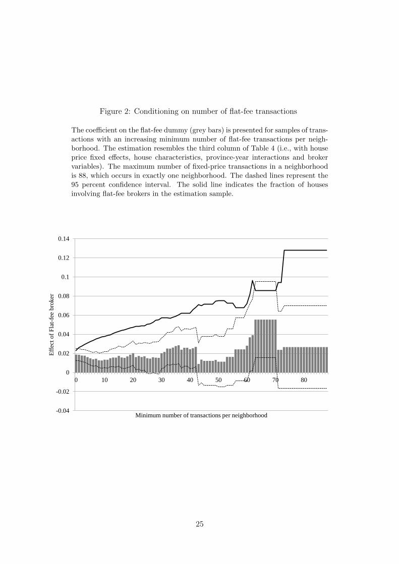
Figure 2: Conditioning on number of flat-fee transactions

The coefficient on the flat-fee dummy (grey bars) is presented for samples of trans-actions with an increasing minimum number of flat-fee transactions per neigh-borhood. The estimation resembles the third column of Table 4 (i.e., with houseprice fixed effects, house characteristics, province-year interactions and brokervariables). The maximum number of fixed-price transactions in a neighborhoodis 88, which occurs in exactly one neighborhood. The dashed lines represent the95 percent confidence interval. The solid line indicates the fraction of housesinvolving flat-fee brokers in the estimation sample.

-0.04

-0.02

0

0.02

0.04

0.06

0.08

0.1

0.12

0.14

0 10 20 30 40 50 60 70 80

Eff

ect

of

Fla

t-fe

e b

rok

er

Minimum number of transactions per neighborhood

25

with the house or neighborhood.

6 Discussion

Houses sold with flat-fee agents seem to exhibit a consistent pattern: (i) they sell at

a higher transaction price and (ii) they sell faster. Proximity, experience, and size

of the broker have no effect on the realized transaction price, and only a negligible

effect on the time to sale. Below, we discuss several potential explanations for our

results: (i) market power, (ii) seller selection effects, (iii) asymmetric information,

and (iv) broker incentives.

6.1 Market power of brokers

The fact that a flat fee leads to better sales performance suggests that the market for

traditional real-estate agents is not competitive. We are hardly the first to point this

out; see for example, Levitt and Syverson (2008a) and Bernheim and Meer (2013).

Even in the financial industry there is clear evidence of persistent inefficiency in the

allocation of retail investor funds to mutual funds; see Del Guercio et al. (2010).

The explanation of limited financial literacy by clients is potentially magnified in the

housing market, which consists of high-stakes transactions that participants engage

in only a few times in their lifetime.

6.2 Seller selection effects

The main alternative explanation for our large effect of using a flat-fee broker is that

what we measure is driven by the selection of sophisticated sellers. In our robustness

section we did not, however, find any evidence for this.

26

Similar issues play a role in the demand for full-service brokers within US

defined-contribution plans; see Chalmers and Reuter (2013). The participants who

use a broker are usually younger, lower educated and less comfortable with making

financial decisions. The specific selection effect that comes with age is also reported

by Agarwal et al. (2009), who find that, across many financial decisions, people

make the best decisions around the age of 53. Our estimations therefore use a

control variable that captures the number of years between sales although this only

partly captures the age-effect of the seller. If sellers are on average older than buyers,

then an age-induced choice for a cheaper (or more efficient) broker might correlate

with better sales performance.

Another potential selection effect is that sellers with high opportunity costs

for conducting the viewings choose a traditional broker to do it for them. However,

based on the price difference of 2.7 percent and a transaction fee for the traditional

real-estate agents of 2 percent, our results indicate a difference of roughly 5 percent of

the sales price. For an average sales price of 200,000 Euro, this implies a difference of

10,000 Euro in terms of the two different types of brokers. It is unlikely that almost

98 percent of the sellers (i.e. those using a traditional real-estate broker), have such

a high level of opportunity costs. To place the 10,000 Euro into perspective, note

that the marginal tax rate in the Netherlands equals 42 percent for a median income

of 35,000 in 2015. Hence, this explanation requires that the opportunity costs must

be roughly half a year of labor income, which seems unlikely.

Better negotiation skills by some sellers, or tougher bargaining are not likely

explanations because both types of brokers advise on the list price and perform the

negotiations at arms-length. Also, we find that using a flat fee has a similar effect

on list prices as on transaction prices; it is therefore not the case that list prices are

27

used more strategically by one type of broker. Finally, as reported in the previous

section, our findings hold for different subsets of sellers and neighborhoods.

6.3 Mitigation of Asymmetric Information

Under the flat-fee structure, sellers are responsible for the viewings themselves. The

personal interaction of hosting the viewings could convey information that decreases

the asymmetric information problem. The face-to-face interaction between buyer

and seller, and the factual knowledge about the house and the neighborhood may

induce the buyer to pay more for the house than when faced with a broker. Lewis

(2011) finds that the market for cars on eBay functions, largely because sellers give

concrete and verifiable information about the particular car they are selling. In the

housing market, viewings hosted by the seller could have the same effect: the seller

can provide details on maintenance and neighborhood characteristics that a typical

real-estate agent would find much harder to provide. Note that this explanation is

consistent with a non-competitive real-estate market.

6.4 Broker specialization

The better performance of flat-fee brokers could reflect a more efficient division of

labor: flat-fee brokers specialize in the skills that are most relevant for transaction

performance, such as price setting, salesmanship and negotiation. The seller takes

on the labor-intensive, but low-skilled, work of hosting viewings, generally providing

better information about the house and displaying some salesmanship. In addition,

the variable costs of rejecting an offer are lower than for full-service brokers, as

the costs of organizing and conducting the viewings are borne by the seller and

28

not the agent. The lower opportunity costs of rejecting an offer could explain why

transaction prices are higher using a flat fee.

Note that the last two explanations imply a potential efficiency gain that

remains largely unexploited, given the low market share of flat-fee brokers – the

persistence of which could be explained by limited attention, limited rationality,

inexperience of sellers or a combination of these factors. The existence of persistent

inefficiency in a competitive market is not impossible, as documented by Cho and

Rust (2010), who find this in the rental car market.

7 Final remarks

After an online centralized listing service for real estate was introduced in 2001, it

became profitable for flat-fee brokers to enter the Dutch market. Brokers charge the

flat fee up-front and delegate the viewings to the sellers. Flat-fee brokers are thus a

low-cost alternative to traditional full-service brokers. Our analysis provides a strong

statistical evidence that the performance of flat-fee brokers is better: they obtain

higher sales prices, at lower sales times. Consequently, the profits of traditional

full-service brokers partly reflect rents.

The existence of a large rent-seeking component in the compensation of tradi-

tional brokers is consistent with limited price competition. The strong performances

of flat-fee brokers has not (yet) eliminated traditional brokers, possibly due to lim-

ited attention and inexperience of sellers in the housing market.

29

References

Agarwal, S., J.C. Driscoll, X. Gabaix and D. Laibson (2009). “The age of

reason: Financial decisions over the life cycle and implications for regulation”,

Brookings Papers on Economic Activity, Fall 2009, 51–117.

Albrecht, J., P.A. Gautier and S. Vroman (2016), “Directed search in the

housing market”, Review of Economic Dynamics, 19, 218–31.

Bergstresser, D., J.M. Chalmers and P. Tufano (2009), “Assessing the

costs and benefits of brokers in the mutual fund industry” Review of Financial

Studies, 22, 4129–56.

Bernheim, B.D. and J. Meer (2013), “Do real estate brokers add value when

listing services are unbundled?”, Economic Inquiry, 51, 1166–82.

Butler, A.W. (2008), “Distance still matters: Evidence from municipal bond

underwriting”, Review of Financial Studies, 21, 763–84.

Case, K.E. and R.J. Shiller (1989), “The efficiency of the market for single-

family homes”, American Economic Review, 79, 125–37.

Cho, S. and J. Rust (2010), “The flat rental puzzle”, Review of Economics

Studies, 77, 560–94.

Coles, M.G., and E. Smith (1998), “Marketplaces and matching”, International

Economic Review, 39, 239–54.

Chalmers, J. and J. Reuter (2013), “What is the impact of financial advisors on

retirement portfolio choices and outcomes?”, working paper, Boston College.

Del Guercio, D., J. Reuter and P.A. Tkac (2010), “Broker incentives and

30

mutual fund market segmentation”, working paper, Boston College.

Gautier, P.A., A.H. Siegmann, A.P. van Vuuren (2009), “Terrorism and

attitudes towards minorities: The effect of the Theo van Gogh murder on

house prices in Amsterdam”, Journal of Urban Economics, 65, 113–26.

Han, L. and S.H. Hong (2011), “Testing cost inefficiency under free entry in the

real estate brokerage industry”, Journal of Business and Economic Statistics,

29, 564–78.

Hendel, I., A. Nevo and F. Ortalo-Magne (2009), “The relative perfor-

mance of real estate marketing platforms: MLS versus FSBOmadison.com”,

American Economic Review, 99, 1878–98.

Ivkovic, Z. and S. Weisbenner (2005), “Local does as local is: Information

content of the geography of individual investors’ common stock investments”,

The Journal of Finance, 60, 267-306.

Levitt, S. and C. Syverson (2008a), “Antitrust implications of home seller

outcomes when using flat-fee real estate agents”, working paper, University of

Chicago.

Levitt, S. and C. Syverson (2008b), “Market distortions when agents are better

informed: The value of information in real estate transactions”, Review of

Economics and Statistics, 90, 599–611.

Lewis, G. (2011), “Asymmetric information, adverse selection and online disclo-

sure: The case of eBay motors” American Economic Review, 101, 1535–46.

Nadel, M. (2006), “A critical assessment of the traditional real estate broker

commission rate structure”, Cornell Real Estate Review, 5, 26-46.

31

OECD (2007), “Improving competition in real estate transactions”, Paris.

Oyer, P. (1998), “Fiscal year ends and nonlinear incentive contracts: The effect

on business seasonality” Quarterly Journal of Economics, 13, 149–85.

Rutherford, R. and A. Yavas (2012), “Discount brokerage in residential real

estate markets, Real Estate Economics, 40, 508-35.

Rutherford, R.C., T. Springer and A. Yavas (2005), “Conflicts between

principals and agents: Evidence from residential brokerage”, Journal of Fi-

nancial Economics, 76, 627–65.

Stacey, D.G. (2013), “Information, commitment, and separation in illiquid hous-

ing markets”, working paper, Ryerson University, Toronto,.

Teo, M. (2009), “The geography of hedge funds”, Review of Financial Studies, 22,

3531–61.

White, L.J. (2006), “The residential real estate brokerage industry: What would

more vigorous competition look like?”, working paper, New York University.

32