RDF User Guide
120
Oracle ® Retail Demand Forecasting User Guide Release 13.0 April 2008
-
Upload
varachartered283 -
Category
Documents
-
view
219 -
download
0
Transcript of RDF User Guide

8/10/2019 RDF User Guide
http://slidepdf.com/reader/full/rdf-user-guide 1/120
Oracle ® Retail Demand Forecasting
User GuideRelease 13.0
April 2008

8/10/2019 RDF User Guide
http://slidepdf.com/reader/full/rdf-user-guide 2/120
Oracle ® Demand Forecasting User Guide, Release 13.0
Copyright © 2008, Oracle. All rights reserved.
Primary Author: Melody CrowleyThe Programs (which include both the software and documentation) contain proprietaryinformation; they are provided under a license agreement containing restrictions on use anddisclosure and are also protected by copyright, patent, and other intellectual and industrialproperty laws. Reverse engineering, disassembly, or decompilation of the Programs, except to theextent required to obtain interoperability with other independently created software or as specified
by law, is prohibited.
The information contained in this document is subject to change without notice. If you find anyproblems in the documentation, please report them to us in writing. This document is notwarranted to be error-free. Except as may be expressly permitted in your license agreement forthese Programs, no part of these Programs may be reproduced or transmitted in any form or byany means, electronic or mechanical, for any purpose.
If the Programs are delivered to the United States Government or anyone licensing or using thePrograms on behalf of the United States Government, the following notice is applicable:
U.S. GOVERNMENT RIGHTS Programs, software, databases, and related documentation andtechnical data delivered to U.S. Government customers are "commercial computer software" or"commercial technical data" pursuant to the applicable Federal Acquisition Regulation and agency-specific supplemental regulations. As such, use, duplication, disclosure, modification, andadaptation of the Programs, including documentation and technical data, shall be subject to thelicensing restrictions set forth in the applicable Oracle license agreement, and, to the extentapplicable, the additional rights set forth in FAR 52.227-19, Commercial Computer Software—Restricted Rights (June 1987). Oracle Corporation, 500 Oracle Parkway, Redwood City, CA 94065
The Programs are not intended for use in any nuclear, aviation, mass transit, medical, or otherinherently dangerous applications. It shall be the licensee's responsibility to take all appropriatefail-safe, backup, redundancy and other measures to ensure the safe use of such applications if the
Programs are used for such purposes, and we disclaim liability for any damages caused by suchuse of the Programs.
Oracle, JD Edwards, PeopleSoft, and Siebel are registered trademarks of Oracle Corporationand/or its affiliates. Other names may be trademarks of their respective owners.
The Programs may provide links to Web sites and access to content, products, and services fromthird parties. Oracle is not responsible for the availability of, or any content provided on, third-party Web sites. You bear all risks associated with the use of such content. If you choose topurchase any products or services from a third party, the relationship is directly between you andthe third party. Oracle is not responsible for: (a) the quality of third-party products or services; or(b) fulfilling any of the terms of the agreement with the third party, including delivery of productsor services and warranty obligations related to purchased products or services. Oracle is notresponsible for any loss or damage of any sort that you may incur from dealing with any thirdparty.
8/10/2019 RDF User Guide
http://slidepdf.com/reader/full/rdf-user-guide 3/120
iii
Value-Added Reseller (VAR) Language
(i) the software component known as ACUMATE developed and licensed by Lucent TechnologiesInc. of Murray Hill, New Jersey, to Oracle and imbedded in the Oracle Retail PredictiveApplication Server – Enterprise Engine, Oracle Retail Category Management, Oracle Retail ItemPlanning, Oracle Retail Merchandise Financial Planning, Oracle Retail Advanced InventoryPlanning and Oracle Retail Demand Forecasting applications.(ii) the MicroStrategy Components developed and licensed by MicroStrategy Services Corporation(MicroStrategy) of McLean, Virginia to Oracle and imbedded in the MicroStrategy for Oracle RetailData Warehouse and MicroStrategy for Oracle Retail Planning & Optimization applications.
(iii) the SeeBeyond component developed and licensed by Sun MicroSystems, Inc. (Sun) of SantaClara, California, to Oracle and imbedded in the Oracle Retail Integration Bus application.
(iv) the Wavelink component developed and licensed by Wavelink Corporation (Wavelink) ofKirkland, Washington, to Oracle and imbedded in Oracle Retail Store Inventory Management.
(v) the software component known as Crystal Enterprise Professional and/or Crystal ReportsProfessional licensed by Business Objects Software Limited (“Business Objects”) and imbedded inOracle Retail Store Inventory Management.
(vi) the software component known as Access Via™ licensed by Access Via of Seattle, Washington,and imbedded in Oracle Retail Signs and Oracle Retail Labels and Tags.
(vii) the software component known as Adobe Flex™ licensed by Adobe Systems Incorporated ofSan Jose, California, and imbedded in Oracle Retail Promotion Planning & Optimizationapplication.
(viii) the software component known as Style Report™ developed and licensed by InetSoftTechnology Corp. of Piscataway, New Jersey, to Oracle and imbedded in the Oracle Retail ValueChain Collaboration application.
(ix) the software component known as WebLogic™ developed and licensed by BEA Systems, Inc.of San Jose, California, to Oracle and imbedded in the Oracle Retail Value Chain Collaborationapplication.
(x) the software component known as DataBeacon™ developed and licensed by CognosIncorporated of Ottawa, Ontario, Canada, to Oracle and imbedded in the Oracle Retail Value ChainCollaboration application.

8/10/2019 RDF User Guide
http://slidepdf.com/reader/full/rdf-user-guide 4/120

8/10/2019 RDF User Guide
http://slidepdf.com/reader/full/rdf-user-guide 5/120
v
ContentsPreface .............................................................................................................................. ix
Audience ................................................................................................................................ ix
Related Documents............................................................................................................... ix
Customer Support................................................................................................................. ix
Review Patch Documentation............................................................................................. ix
Oracle Retail Documentation on the Oracle Technology Network................................ ix
Conventions............................................................................................................................. x
1 Introduction .................................................................................................................. 1
Overview.................................................................................................................................. 1
Forecasting Challenges and RDF Solutions......................................................................... 1
Selecting the Best Forecasting Method ......................................................................... 2
Overcoming Data Sparsity through Source Level Forecasting.................................. 2
Forecasting Demand for New Products and Locations .............................................. 3
Managing Forecasting Results through Automated Exception Reporting.............. 3
Incorporating the Effects of Promotions and Other Event-Based Challenges onDemand............................................................................................................................. 4
Oracle Retail Demand Forecasting Architecture ................................................................ 4
The Oracle Retail Predictive Application Server and RDF ........................................ 4
Global Domain vs. Simple Domain Environnent ........................................................ 5
Oracle Retail Demand Forecasting Workbook Template Groups.................................... 6
Forecast.............................................................................................................................. 6
Promote (Promotional Forecasting) .............................................................................. 6
Curve ................................................................................................................................. 7
RDF Solution and Business Process Overview................................................................... 7
RDF and the Oracle Retail Enterprise ........................................................................... 7
RDF Primary Workflow.................................................................................................. 7
2 Setting Forecast Parameters ...................................................................................... 9
Overview.................................................................................................................................. 9
Forecast Administration Workbook Overview ........................................................... 9
Forecast Administration Workbook................................................................................... 12
Creating a Forecast Administration Workbook......................................................... 12
Window Descriptions.................................................................................................... 12
Forecast Maintenance Workbook ....................................................................................... 27
Overview......................................................................................................................... 27
Creating a Forecast Maintenance Workbook............................................................. 27
Window Descriptions.................................................................................................... 28
Forecast Like-Item, Sister-Store Workbook....................................................................... 31
Overview......................................................................................................................... 31
Creating a Forecast Like-Item, Sister-Store Workbook............................................. 32
Window Descriptions.................................................................................................... 33
8/10/2019 RDF User Guide
http://slidepdf.com/reader/full/rdf-user-guide 6/120
vi
Steps Required for Forecasting Using Each of the Like SKU / Sister StoreMethods........................................................................................................................... 37
Product/Location Cloning Administration Workbook................................................... 39
Overview......................................................................................................................... 39
Window Descriptions.................................................................................................... 40
3 Generating and Approving a Forecast .................................................................... 45 Overview................................................................................................................................ 45
Run a Batch Forecast............................................................................................................. 45
Overview......................................................................................................................... 45
Procedures ...................................................................................................................... 46
Delete Forecasts..................................................................................................................... 46
Overview......................................................................................................................... 46
Permanently Removing a Forecast from the Oracle Retail Demand ForecastingSystem ............................................................................................................................. 46
Forecast Approval Workbook............................................................................................. 47
Overview......................................................................................................................... 47
Opening or Creating the Forecast Approval Workbook .......................................... 48
Window Descriptions.................................................................................................... 50
Approving Forecasts through Alerts (Exception Management) .................................... 56
Overview......................................................................................................................... 56
4 Forecast Analysis Tools ........................................................................................... 57
Overview................................................................................................................................ 57
Interactive Forecasting Workbook...................................................................................... 57
Overview......................................................................................................................... 57
Opening the Interactive Forecasting Workbook........................................................ 57
Window Descriptions.................................................................................................... 58 Forecast Scorecard Workbook............................................................................................. 60
Overview......................................................................................................................... 60
Opening or Creating a Forecast Scorecard Workbook ............................................. 60
Window Descriptions.................................................................................................... 62
5 Promote (Promotional Forecasting) ........................................................................ 65
Overview................................................................................................................................ 65
What is Promotional Forecasting?............................................................................... 65
Comparison between Promotional and Statistical Forecasting ............................... 66
Developing Promotional Forecast Methods............................................................... 66
Oracle Retail’s Approach to Promotional Forecasting.............................................. 67 Promotional Forecasting Terminology and Workflow............................................. 67
Promote Workbooks and Wizards .............................................................................. 68
Promotion Planner Workbook Template........................................................................... 69
Overview......................................................................................................................... 69
Opening or Creating a Promotion Planner Workbook............................................. 69
Window Descriptions.................................................................................................... 70
8/10/2019 RDF User Guide
http://slidepdf.com/reader/full/rdf-user-guide 7/120
vii
Promotion Maintenance Workbook Template.................................................................. 70
Overview......................................................................................................................... 70
Opening the Promotion Maintenance Workbook Template.................................... 71
Window Descriptions.................................................................................................... 71
Promotion Effectiveness Workbook Template ................................................................. 73
Overview......................................................................................................................... 73 Opening the Promotion Effectiveness Workbook Template ................................... 74
Window Descriptions........................................................................................................... 74
Procedures in Promotional Forecasting............................................................................. 77
Setting Up the System to Run a Promotional Forecast ............................................. 78
Viewing a Forecast that Includes Promotion Effects ................................................ 78
Viewing and Editing Promotion System-Calculated Effects ................................... 79
Promotion Simulation (“what-if?”) and Analysis ..................................................... 79
6 Oracle Retail Demand Forecasting Methods .......................................................... 81
Forecasting Techniques Used in RDF ................................................................................ 81
Exponential Smoothing................................................................................................. 81
Regression Analysis....................................................................................................... 81
Bayesian Analysis .......................................................................................................... 81
Prediction Intervals ....................................................................................................... 82
Automatic Method Selection........................................................................................ 82
Source Level Forecasting .............................................................................................. 82
Promotional Forecasting............................................................................................... 82
Time Series (Statistical) Forecasting Methods................................................................... 83
Why Use Statistical Forecasting? ................................................................................. 83
Exponential Smoothing (ES) Forecasting Methods................................................... 84
Average ........................................................................................................................... 84 Simple Exponential Smoothing.................................................................................... 85
Croston’s Method .......................................................................................................... 85
Simple/Intermittent Exponential Smoothing............................................................ 85
Holt Exponential Smoothing........................................................................................ 86
Multiplicative Winters Exponential Smoothing ........................................................ 86
Additive Winters Exponential Smoothing ................................................................. 89
Seasonal Exponential Smoothing (SeasonalES)......................................................... 89
Seasonal Regression....................................................................................................... 90
Bayesian Information Criterion (BIC) ......................................................................... 90
Profile-Based Forecasting..................................................................................................... 95 Forecast Method............................................................................................................. 95
Profile-Based Method and New Items........................................................................ 96
Bayesian Forecasting ............................................................................................................ 96
Sales Plans vs. Historic Data ........................................................................................ 97
Bayesian Algorithm....................................................................................................... 97
Causal (Promotional) Forecasting Method........................................................................ 98

8/10/2019 RDF User Guide
http://slidepdf.com/reader/full/rdf-user-guide 8/120
viii
The Causal Forecasting Algorithm.............................................................................. 99
Causal Forecasting Algorithm Process ....................................................................... 99
Causal Forecasting at the Daily Level ....................................................................... 102
Final Considerations about Causal Forecasting ...................................................... 103
Glossary......................................................................................................................... 105
8/10/2019 RDF User Guide
http://slidepdf.com/reader/full/rdf-user-guide 9/120
ix
PrefaceThe Oracle Retail Demand Forecasting User Guide describes the application’s user interfaceand how to navigate through it.
AudienceThis document is intended for the users and administrators of Oracle Retail DemandForecasting. This may include merchandisers, buyers, and business analysts.
Related DocumentsFor more information, see the following documents in the Oracle Retail DemandForecasting Release 13.0 documentation set: Oracle Retail Demand Forecasting Release Notes Oracle Retail Demand Forecasting Installation Guide Oracle Retail Demand Forecasting Administration Guide Oracle Retail Demand Forecasting Configuration Guide Oracle Retail Predictive Application Server documentation
Customer Support https://metalink.oracle.com
When contacting Customer Support, please provide: Product version and program/module name. Functional and technical description of the problem (include business impact). Detailed step-by-step instructions to recreate. Exact error message received. Screen shots of each step you take.
Review Patch DocumentationFor a base release (".0" release, such as 13.0), Oracle Retail strongly recommends that youread all patch documentation before you begin installation procedures. Patchdocumentation can contain critical information related to the base release, based on newinformation and code changes that have been made since the base release.
Oracle Retail Documentation on the Oracle Technology NetworkIn addition to being packaged with each product release (on the base or patch level), allOracle Retail documentation is available on the following Web site:http://www.oracle.com/technology/documentation/oracle_retail.html Documentation should be available on this Web site within a month after a productrelease. Note that documentation is always available with the packaged code on therelease date.

8/10/2019 RDF User Guide
http://slidepdf.com/reader/full/rdf-user-guide 10/120
x
ConventionsNavigate: This is a navigate statement. It tells you how to get to the start of the procedureand ends with a screen shot of the starting point and the statement “the Window Namewindow opens.”
Note: This is a note. It is used to call out information that isimportant, but not necessarily part of the procedure.
Thi s i s a code sampl eI t i s used t o di spl ay exampl es of code
A hyperlink appears like this .
8/10/2019 RDF User Guide
http://slidepdf.com/reader/full/rdf-user-guide 11/120
Introduction 1
1Introduction
OverviewOracle Retail Demand Forecasting is a Windows-based statistical and promotionalforecasting solution. It uses state-of-the-art modeling techniques to produce high qualityforecasts with minimal human intervention. Forecasts produced by the DemandForecasting system enhance the retailer’s supply-chain planning, allocation, andreplenishment processes, enabling a profitable and customer-oriented approach topredicting and meeting product demand.Today’s progressive retail organizations know that store-level demand drives the supplychain. The ability to forecast consumer demand productively and accurately is vital to aretailer’s success. The business requirements for consumer responsiveness mandate aforecasting system that more accurately forecasts at the point of sale, handles difficultdemand patterns, forecasts promotions and other causal events, processes large numbersof forecasts, and minimizes the cost of human and computer resources.Forecasting drives the business tasks of planning, replenishment, purchasing, andallocation. As forecasts become more accurate, businesses run more efficiently by buyingthe right inventory at the right time. This ultimately lowers inventory levels, improvessafety stock requirements, improves customer service, and increases the company’sprofitability.The competitive nature of business requires that retailers find ways to cut costs andimprove profit margins. The accurate forecasting methodologies provided with OracleRetail Demand Forecasting can provide tremendous benefits to businesses.A connection from Oracle Retail Demand Forecasting to Oracle Retail’s Advanced RetailPlanning and Optimization (ARPO) solutions is built directly into the business process
by way of the automatic approvals of forecasts, which may then fed directly to anyARPO solution. This process allows you to accept all or part of a generated sales forecast.Once that decision is made, the remaining business measures may be planned within anARPO solution such as Merchandise Financial Planning, for example.
Forecasting Challenges and RDF SolutionsA number of challenges affect the ability of organizations to forecast product demandaccurately. These challenges include selecting the best forecasting method to account forlevel, trending, seasonal, and spiky demand; generating forecasts for items with limiteddemand histories; forecasting demand for new products and locations; incorporating theeffects of promotions and other event-based challenges on demand; and accommodatingthe need of operational systems to have sales predictions at more detailed levels than
planning programs provide.

8/10/2019 RDF User Guide
http://slidepdf.com/reader/full/rdf-user-guide 12/120
Forecasting Challenges and RDF Solutions
2 Oracle Retail Demand Forecasting
Selecting the Best Forecasting MethodOne challenge to accurate forecasting is the selection of the best model to account forlevel, trending, seasonal, and spiky demand. Oracle Retail’s AutoES (AutomaticExponential Smoothing) forecasting method eliminates this complexity.The AutoES method evaluates multiple forecast models, such as Simple Exponential
Smoothing, Holt Exponential Smoothing, Additive and Multiplicative WintersExponential Smoothing, Croston’s Intermittent Demand Model, and Seasonal Regressionforecasting to determine the optimal forecast method to use for a given set of data. Theaccuracy of each forecast and the complexity of the forecast model are evaluated in orderto determine the most accurate forecast method. You simply select the AutoES forecastgeneration method and the system finds the best model.
Overcoming Data Sparsity through Source Level ForecastingIt is a common misconception in forecasting that forecasts must be directly generated atthe lowest levels (final levels) of execution. Problems can arise when historic sales datafor these items is too sparse and noisy to identify clear selling patterns. In such cases,generating a reliable forecast requires aggregating sales data from a final level up to a
higher level (source level) in the hierarchy in which demand patterns can be seen, andthen generate a forecast at this source level. After a forecast is generated at the sourcelevel, the resulting data can be allocated (spread) back down to the lower level based onthe lower level’s (final level) relationship to the total. This relationship can then bedetermined through generating an additional forecast (interim forecast) at the final level.Curve is then used to dynamically generate a profile based on the interim forecasts. Aswell, a non-dynamic profile can be generated and approved to be used as this profile. It isthis profile that determines how the source level forecast is spread down to the finallevel. For more information on Curve, see the Curve User Guide.

8/10/2019 RDF User Guide
http://slidepdf.com/reader/full/rdf-user-guide 13/120
Forecasting Challenges and RDF Solutions
Introduction 3
Some high-volume items may possess sufficient sales data for robust forecast calculationsdirectly at the final forecast level. In these cases, forecast data generated at an aggregatelevel and then spread down to lower levels can be compared to the interim forecasts rundirectly at the final level. Comparing the two forecasts, each generated at a differenthierarchy level, can be an invaluable forecast performance evaluation tool.Your Oracle Retail Demand Forecasting system may include multiple final forecastlevels. Forecast data must appear at a final level for the data to be approved and exportedto another system for execution.
Forecasting Demand for New Products and LocationsOracle Retail Demand Forecasting also forecasts demand for new products and locationsfor which no sales history exists. You can model a new product’s demand behavior basedon that of an existing similar product for which you do have a history. Forecasts can begenerated for the new product based on the history and demand behavior of the existingone. Likewise, the sales histories of existing store locations can be used as the forecastfoundation for new locations in the chain. For more details, see the section on ForecastLike-Item, Sister-Store Workbook.
Managing Forecasting Results through Automated Exception ReportingThe RDF end user may be responsible for managing the forecast results for thousands ofitems, at hundreds of stores, across many weeks at a time. The Oracle Retail PredictiveApplication Server (RPAS) provides users with an automated exception reportingprocess (called Alert Management) that indicates to the user where a forecast value maylie above or below an established threshold, thereby reducing the level of interactionneeded from the user.Alert management is a feature that provides user-defined and user-maintained exceptionreporting. Through the process of alert management, you define measures that arechecked daily to see if any values fall outside of an acceptable range or do not match agiven value. When this happens, an alert is generated to let you know that a measuremay need to be examined and possibly amended in a workbook.The Alert Manager is a dialog box that is displayed automatically when you log on to thesystem. This dialog provides a list of all identified instances in which a given measure’svalues fall outside of the defined limits. You may pick an alert from this list and have thesystem automatically build a workbook containing that alert’s measure. In the workbook,you can examine the actual measure values that triggered the alert and make decisionsabout what needs to be done next.For more information on the Alert Manager, see the RPAS User Guide .

8/10/2019 RDF User Guide
http://slidepdf.com/reader/full/rdf-user-guide 14/120
Oracle Retail Demand Forecasting Architecture
4 Oracle Retail Demand Forecasting
Incorporating the Effects of Promotions and Other Event-Based Challenges on DemandPromotions, non-regular holidays, and other causal events create another significantchallenge to accurate forecasting. Promotions such as advertised sales and free gifts withpurchase might have a significant impact on a product’s sales history, as can irregularlyoccurring holidays such as Easter.
Using Promotional Forecasting (an optional, add-on module to Oracle Retail DemandForecasting), promotional models of forecasting can be developed to take these and otherfactors into account when forecasts are generated. Promotional Forecasting attempts toidentify the causes of deviations from the established seasonal profile, quantify theseeffects, and use the results to predict future sales when conditions in the sellingenvironment will be similar. This type of advanced forecasting identifies the behavioralrelationship of the variable you want to forecast (sales) to both its own past andexplanatory variables such as promotion and advertising.Suppose that your company has a large promotional event during the Easter season eachyear. The exact date of the Easter holiday varies from year to year; as a result, thestandard time-series forecasting model often has difficulty representing this effect in theseasonal profile. The Promotional Forecasting module allows you to identify the Easterseason in all years of your sales history, and then define the upcoming Easter date. Bydoing so, you can causally forecast the Easter-related demand pattern shift.
Oracle Retail Demand Forecasting Architecture
The Oracle Retail Predictive Application Server and RDFThe Oracle Retail Demand Forecasting application is a member of the Advanced RetailPlanning and Optimization Suite (ARPO), including other solutions such as MerchandiseFinancial Planning, Item Planning, Category Management, and Advance InventoryPlanning. The ARPO solutions share a common platform called the Oracle RetailPredictive Application Server (RPAS). RDF leverages the versatility, power, and speed ofthe RPAS engine and user-interface. Features such as the following characterize RPAS:
Multidimensional databases and database components (dimensions, positions,hierarchies)
Product, location, and calendar hierarchies Aggregation and spreading of sales data Client-server architecture and master database Workbooks and worksheets for displaying and manipulating forecast data Wizards for creating and formatting workbooks and worksheets Menus, quick menus, and toolbars for working with sales and forecast data An automated alert system that provides user-defined and user-maintained
exception reporting Charting and graphing capabilities
More details about the use of these features can be found in the RPAS User Guide andonline help provided within your RDF solution.
8/10/2019 RDF User Guide
http://slidepdf.com/reader/full/rdf-user-guide 15/120
Oracle Retail Demand Forecasting Architecture
Introduction 5
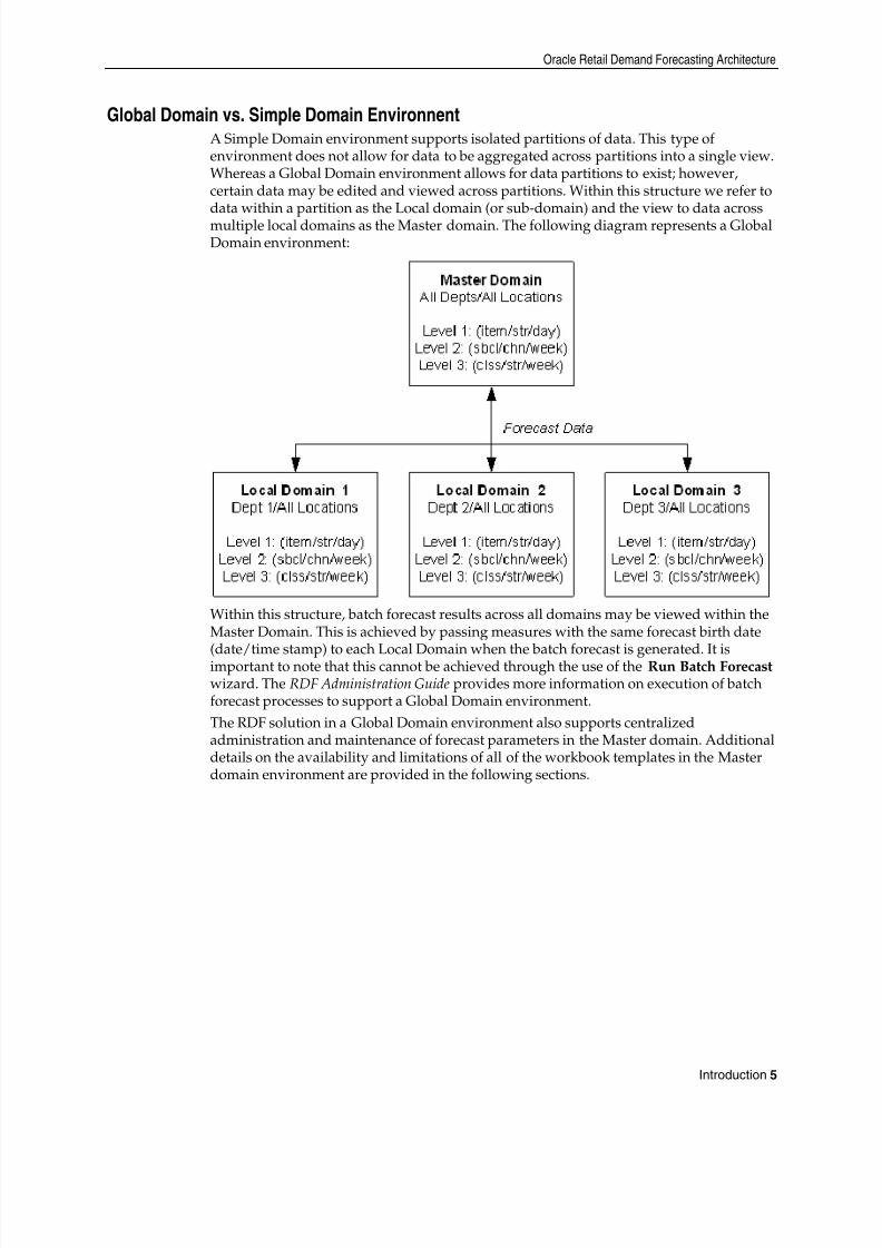
Global Domain vs. Simple Domain EnvironnentA Simple Domain environment supports isolated partitions of data. This type ofenvironment does not allow for data to be aggregated across partitions into a single view.Whereas a Global Domain environment allows for data partitions to exist; however,certain data may be edited and viewed across partitions. Within this structure we refer todata within a partition as the Local domain (or sub-domain) and the view to data acrossmultiple local domains as the Master domain. The following diagram represents a GlobalDomain environment:
Within this structure, batch forecast results across all domains may be viewed within theMaster Domain. This is achieved by passing measures with the same forecast birth date
(date/time stamp) to each Local Domain when the batch forecast is generated. It isimportant to note that this cannot be achieved through the use of the Run Batch Forecast wizard. The RDF Administration Guide provides more information on execution of batchforecast processes to support a Global Domain environment.The RDF solution in a Global Domain environment also supports centralizedadministration and maintenance of forecast parameters in the Master domain. Additionaldetails on the availability and limitations of all of the workbook templates in the Masterdomain environment are provided in the following sections.

8/10/2019 RDF User Guide
http://slidepdf.com/reader/full/rdf-user-guide 16/120
Oracle Retail Demand Forecasting Workbook Template Groups
6 Oracle Retail Demand Forecasting
Oracle Retail Demand Forecasting Workbook Template GroupsIn addition to the standard RPAS Administration and Analysis Workbook TemplateGroups, there are several template groups that are associated with the Oracle RetailDemand Forecasting solution may include: Forecast, Promote, Curve or any ARPOsolution (available modules are based upon licensing agreement).
New Dialog Box
ForecastThe Forecast module refers to the primary RDF functionality and consists of theworkbook templates, measures, and forecasting algorithms that are needed to performtime-series forecasting. This includes the Forecast Administration, Forecast Maintenance,Forecast Like-Item, Sister-Store, Run Batch Forecast, Forecast Approval, ForecastScorecard, Interactive Forecasting, and Delete Forecast Workbook templates. TheForecast module also includes the batch forecasting routine and all of its componentalgorithms.
Promote (Promotional Forecasting)The Promote module consists of the templates and algorithms required to performpromotional forecasting, which uses both past sales data and promotional information
(for example, advertisements, holidays) to forecast future demand. This module includesthe Promotion Maintenance, Promotion Planner and Promotion Effectiveness templates.
8/10/2019 RDF User Guide
http://slidepdf.com/reader/full/rdf-user-guide 17/120
RDF Solution and Business Process Overview
Introduction 7
CurveThe Curve module consists of the workbook templates and batch algorithms that arenecessary for the creation, approval, and application of profiles that may be used tospread source level forecasts down to final levels as well to generate profiles, which may
be used in any RPAS solution. The types of profiles typically used to support forecastingare: Store Contribution, Product, and Daily profiles. These profiles may also be used tosupport Profile-Based Forecasting; however, Curve may be used to generate profiles thatare used by other ARPO solutions for reasons other than forecasting. Profiles Typesinclude: Daily Seasonal, Lifecycle, Size, Hourly, and User-Defined profiles. For moreinformation on the Curve Workbooks and Worksheets, see the Curve User Guide.
RDF Solution and Business Process Overview
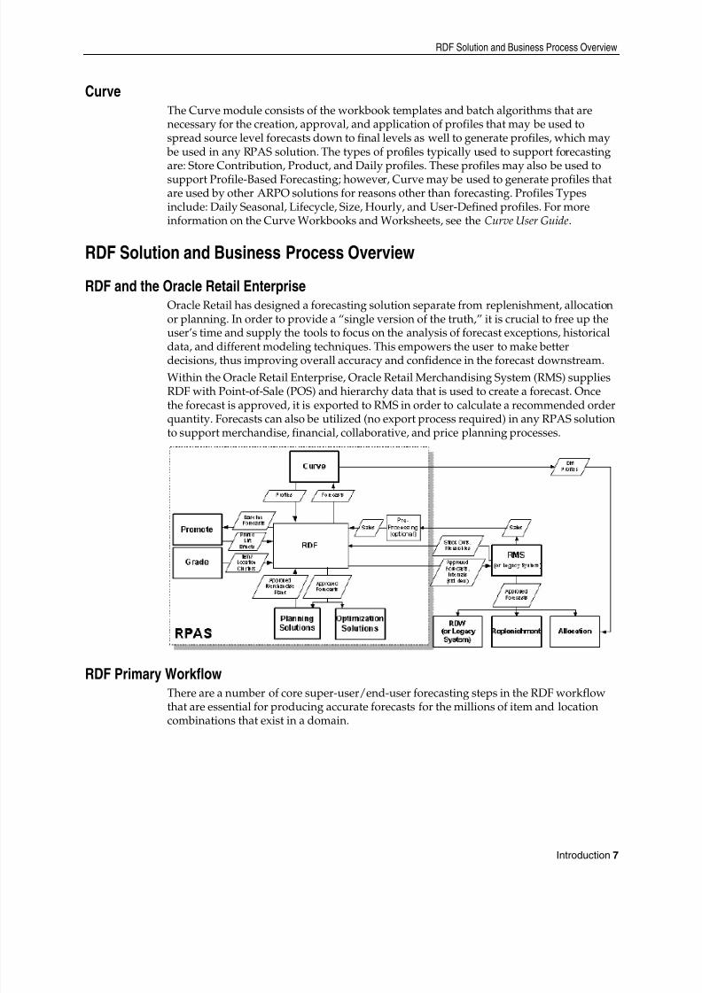
RDF and the Oracle Retail EnterpriseOracle Retail has designed a forecasting solution separate from replenishment, allocationor planning. In order to provide a “single version of the truth,” it is crucial to free up theuser’s time and supply the tools to focus on the analysis of forecast exceptions, historical
data, and different modeling techniques. This empowers the user to make betterdecisions, thus improving overall accuracy and confidence in the forecast downstream.Within the Oracle Retail Enterprise, Oracle Retail Merchandising System (RMS) suppliesRDF with Point-of-Sale (POS) and hierarchy data that is used to create a forecast. Oncethe forecast is approved, it is exported to RMS in order to calculate a recommended orderquantity. Forecasts can also be utilized (no export process required) in any RPAS solutionto support merchandise, financial, collaborative, and price planning processes.
RDF Primary Workflow
There are a number of core super-user/end-user forecasting steps in the RDF workflowthat are essential for producing accurate forecasts for the millions of item and locationcombinations that exist in a domain.

8/10/2019 RDF User Guide
http://slidepdf.com/reader/full/rdf-user-guide 18/120

8/10/2019 RDF User Guide
http://slidepdf.com/reader/full/rdf-user-guide 19/120
8/10/2019 RDF User Guide
http://slidepdf.com/reader/full/rdf-user-guide 20/120
Overview
10 Oracle Retail Demand Forecasting
Forecasting Methods Available in Oracle Retail Demand ForecastingA forecasting system’s main goal is to produce accurate predictions of future demand.Oracle Retail’s Demand Forecasting solution utilizes the most advanced forecastingalgorithms to address many different data requirements across all retail verticals.Furthermore, the system can be configured to automatically select the best algorithm andforecasting level to yield the most accurate results.The following section summarizes the use of the various forecasting methods employedin the system. This section is referenced throughout this document when the selection ofa forecasting method is required in a workflow process. Some of these methods may not
be visible in your solution based on configuration options set in the RPAS ConfigurationTools. More detailed information on these forecasting algorithms is provided in“Forecasting Methods Available in Oracle Retail Demand Forecasting .”
AverageOracle Retail Demand Forecasting uses a simple average model to generate forecasts.
Moving AverageOracle Retail Demand Forecasting uses a simple moving average model to generateforecasts. Users can specify a Moving Average Window length.
AutoESOracle Retail Demand Forecasting fits the sales data to a variety of exponentialsmoothing models of forecasting, and the best model is chosen for the final forecast. Thecandidate methods considered by AutoES are: Simple ES Intermittent ES Trend ES Multiplicative Seasonal Additive Seasonal Seasonal ES
The final selection between the models is made according to a performance criterion(Bayesian Information Criterion) that involves a tradeoff between the model’s fit over thehistoric data and its complexity.
Simple ESOracle Retail Demand Forecasting uses a simple exponential smoothing model togenerate forecasts. Simple ES ignores seasonality and trend features in the demand dataand is the simplest model of the exponential smoothing family. This method can be usedwhen less than one year of historic demand data is available.
Intermittent ESOracle Retail Demand Forecasting fits the data to the Croston's model of exponentialsmoothing. This method should be used when the input series contains a large number ofzero data points (that is, intermittent demand data). The original time series is split into aMagnitude and Frequency series, and then the Simple ES model is applied to determinelevel of both series. The ratio of the magnitude estimate over the frequency estimate isthe forecast level reported for the original series.

8/10/2019 RDF User Guide
http://slidepdf.com/reader/full/rdf-user-guide 21/120
Overview
Setting Forecast Parameters 11
Simple/IntermittentESA combination of the Simple ES and Intermittent ES methods. This method applies theSimple ES model unless a large number of zero data points are present, in which case theCroston’s model is applied.
TrendES
Oracle Retail Demand Forecasting fits the data to the Holt model of exponentialsmoothing. The Holt model is useful when data exhibits a definite trend. This methodseparates base demand from trend, and then provides forecast point estimates bycombining an estimated trend and the smoothed level at the end of the series. Forinstance, where the forecast engine cannot produce a forecast using the Trend ESmethod, the Simple/Intermittent ES method is used to evaluate the time series.
Multiplicative SeasonalAlso referred to as Multiplicative Winters Model, this model extracts seasonal indicesthat are assumed to have multiplicative effects on the un-seasonalized series.
Additive Seasonal
Also referred to as Additive Winters Model, this model is similar to the MultiplicativeWinters model, but is used when zeros are present in the data. This model adjusts the un-seasonalized values by adding the seasonal index (for the forecast horizon).
Seasonal ESThis method, a combination of several Seasonal methods, is generally used for knownseasonal items or forecasting for long horizons. This method applies the MultiplicativeSeasonal model unless zeros are present in the data, in which case the Additive Wintersmodel of exponential smoothing is used. If less than two years of data is available, aSeasonal Regression model is used. If there is too little data to create a seasonal forecast(in general, less than 52 weeks), the system will select from the Simple ES, Trend ES, andIntermittent ES methods.
Seasonal RegressionSeasonal Regression cannot be selected as a forecasting method, but is a candidate modelthat is used only when the Seasonal ES method is selected. This model requires aminimum of 52 weeks of history to determine seasonality. Simple Linear Regression isused to estimate the future values of the series based on a past series. The independentvariable is the series history one-year or one cycle length prior to the desired forecastperiod, and the dependent variable is the forecast. This model assumes that the future isa linear combination of itself one period before plus a scalar constant.
CausalCausal is used for promotional forecasting and can only be selected if Promote is
implemented. Causal uses a Stepwise Regression sub-routine to determine thepromotional variables that are relevant to the time series and their lift effect on the series.AutoES utilizes the time series data and the future promotional calendar to generatefuture baseline forecasts. By combining the future baseline forecast and each promotion’seffect on sales (lift), a final promotional forecast is computed. For instances where theforecasting engine cannot produce a forecast using the Causal method, the system willevaluate the time series using the Seasonal ES method.

8/10/2019 RDF User Guide
http://slidepdf.com/reader/full/rdf-user-guide 22/120
Forecast Administration Workbook
12 Oracle Retail Demand Forecasting
No ForecastNo forecast will be generated for the product/location combination.
BayesianUseful for short lifecycle forecasting and for new products with little or no historic salesdata, the Bayesian method requires a product’s known sales plan (created externally toRDF) and considers a plan’s shape (the selling profile or lifecycle) and scale (magnitudeof sales based on Actuals). The initial forecast is equal to the sales plan, but as salesinformation comes in, the model generates a forecast by merging the sales plan with thesales data. The forecast is adjusted so that the sales magnitude is a weighted average
between the original plan’s scale and the scale reflected by known history. A Data Planmust be specified when using the Bayesian method. For instances where the Data Planequals zero (0), the system will evaluate the time series using the Seasonal ES method.
Profile-basedOracle Retail Demand Forecasting generates a forecast based on a seasonal profile thatcan be created in RPAS or legacy system. Profiles can also be copied from another profileand adjusted. Using historic data and the profile, the data is de-seasonalized and then fed
to the Simple ES method. The Simple forecast is then re-seasonalized using the profiles. ASeasonal Profile must be specified when using the Profile-Based method. For instanceswhere the Seasonal Profile equals zero (0), the system will evaluate the time series usingthe Seasonal ES method.
Forecast Administration Workbook
Creating a Forecast Administration Workbook1. Within the Master or Local Domain, select New from the File menu.2. Select the Forecast tab to display a list of workbook templates for statistical
forecasting.
3. Select Forecast Administration .4. Click OK .5. The Forecast Administration wizard opens and prompts you to select the level of the
final forecast. The final forecast level is a level at which approvals and data exportscan be performed. Depending on your organization’s setup, you may be offered achoice of several final forecast levels. Make the appropriate selection.
6. Click Finish to open the workbook.
Window Descriptions
Basic Settings Workflow Tab
The Basic Settings workflow tab contains forecast administration settings. On the BasicSettings workflow tab, there are two worksheets: Final Level Parameters Worksheet Final and Source Level Parameters Worksheet
8/10/2019 RDF User Guide
http://slidepdf.com/reader/full/rdf-user-guide 23/120
Forecast Administration Workbook
Setting Forecast Parameters 13
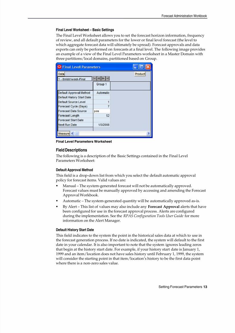
Final Level Worksheet – Basic SettingsThe Final Level Worksheet allows you to set the forecast horizon information, frequencyof review, and all default parameters for the lower or final level forecast (the level towhich aggregate forecast data will ultimately be spread). Forecast approvals and dataexports can only be performed on forecasts at a final level. The following image providesan example of a view of the Final Level Parameters worksheet in a Master Domain withthree partitions/local domains, partitioned based on Group.
Final Level Parameters Worksheet
Field DescriptionsThe following is a description of the Basic Settings contained in the Final LevelParameters Worksheet:
Default Approval Method
This field is a drop-down list from which you select the default automatic approvalpolicy for forecast items. Valid values are: Manual – The system-generated forecast will not be automatically approved.
Forecast values must be manually approved by accessing and amending the ForecastApproval Workbook.
Automatic – The system-generated quantity will be automatically approved as-is. By Alert – This list of values may also include any Forecast Approval alerts that have
been configured for use in the forecast approval process. Alerts are configuredduring the implementation. See the RPAS Configuration Tools User Guide for moreinformation on the Alert Manager.
Default History Start DateThis field indicates to the system the point in the historical sales data at which to use inthe forecast generation process. If no date is indicated, the system will default to the firstdate in your calendar. It is also important to note that the system ignores leading zerosthat begin at the history start date. For example, if your history start date is January 1,1999 and an item/location does not have sales history until February 1, 1999, the systemwill consider the starting point in that item/location’s history to be the first data pointwhere there is a non-zero sales value.

8/10/2019 RDF User Guide
http://slidepdf.com/reader/full/rdf-user-guide 24/120
Forecast Administration Workbook
14 Oracle Retail Demand Forecasting
Default Source LevelThe pick list of values displayed in this field allows the user to change the forecast levelthat will be used as the primary level to generate the source forecast. The source levelsare set up in the RPAS Configuration Tool. A value from the pick list is required in thisfield at the time of forecast generation.
Forecast CycleThe Forecast Cycle is the amount of time (measured in days) that the system waits
between each forecast generation. Once a scheduled forecast has been generated, thisfield is used to automatically update the Next Run Date field. A non-zero value isrequired in this field at the time of forecast generation.
Forecast Data SourceThis is a read-only value that displays the sales measure (the measure name) that will bethe data used for the generation of forecasts (for example, pos). The measure that will bedisplayed here is determined at configuration time in the RPAS Configuration Tools.
Forecast Start Date
This is the starting date of the forecast. If no value is specified at the time of forecastgeneration, the system will use the data/time at which the batch is executed as thedefault value. If a value is specified in this field and it is used to successfully generate the
batch forecast, this value will be cleared.
Forecast LengthThe Forecast Length is used with the Forecast Start Date to determine forecast horizon.The forecast length is based on the calendar dimension of the final level. For example, ifthe forecast length is to be 10 weeks, the setting for a final level at day is 70 (10 x 7 days).
Next Run DateThe Next Run Date is the date on which the next batch forecast generation process will
automatically be run. Oracle Retail Demand Forecasting automatically triggers a set of batch processes to be run at a pre-determined time period. When a scheduled batch isrun successfully, the Next Run Date automatically updates based on the Start Date valueand the Forecast Cycle. No value is required in this field when the Run Batch Forecast wizard is used to generate the forecast or if the batch forecast is run from the backend ofthe domain(s) using the “override true” option. See the RDF Administration Guide formore information on forecast generation.

8/10/2019 RDF User Guide
http://slidepdf.com/reader/full/rdf-user-guide 25/120
Forecast Administration Workbook
Setting Forecast Parameters 15
Final and Source Level Parameters Worksheet – Basic SettingsThe Final and Source Level Worksheet allows you to set the default parameters that arecommon to both the final and source level forecasts.
Final and Source Level Parameters Worksheet
Field DescriptionsThe following is a description of the Basic Settings parameters contained in the SourceLevel Worksheet:
Data PlanUsed in conjunction with the Bayesian forecast method, Data Plan is used to input themeasure name of a sales plan that should be associated with the final level forecast. Salesplans, when available, provide details of the anticipated shape and scale of an item’sselling pattern. If the Data Plan is required, this field should include the measure nameassociated with the Data Plan.
Default Forecast MethodThe Default Forecast Method is a drop-down list from which you can select the primaryforecast method that will be used to generate the forecast. Valid method options dependon your system setup. A summary of methods is provided earlier in this chapter and thelast chapter in this guide covers each method in greater detail. It is important to note thatCausal should not be selected unless the forecast level was set as a Causal level duringthe configuration. See the RDF Configuration Guide for more information onconfigurations using the Causal forecast method.
Seasonal ProfileUsed in conjunction with the Profile-Based forecasting method, this is the measure nameof the seasonal profile that will be used to generate the forecast at either the source orfinal level. Seasonal profiles, when available, provide details of the anticipatedseasonality (shape) of an item’s selling pattern. The seasonal profile can be generated orloaded, depending on your configuration. The original value of this measure is setduring the configuration of the RDF solution.

8/10/2019 RDF User Guide
http://slidepdf.com/reader/full/rdf-user-guide 26/120
Forecast Administration Workbook
16 Oracle Retail Demand Forecasting
Spreading ProfileUsed for Source Level Forecasting, the value of this measure indicates the profile levelthat will be used to determine how the source level forecast is spread down to the finallevel. No value is needed to be entered at the final level. For dynamically generatedprofiles, this value is the number associated with the final profile level (for example 01)—note that profiles 1 through 9 have a zero (0) preceding them in Curve—this is differentthan the forecasting level numbers. For profiles that must be approved, this is themeasure associated with the final profile level. This measure is defined as “apvp”+level(for example: apvp01 for the approved profile for level 01 in Curve).
Advanced Settings Workflow TabThe Forecast Administration Advanced Settings workflow tab is used to set parametersrelated to either the data that is stored in the system or the forecasting methods that will
be used at the final or source levels. The parameters on this workflow tab are not as likelyto be changed on a regular basis as the ones on the Basic Settings workflow tab.
Final Level Parameters Worksheet – Advanced SettingsThe Final Level Worksheet allows you to set the advanced parameters for the final level
forecasts. The following image provides an example of a view of this worksheet in aMaster Domain with three partitions/Local Domains, partitioned based on Group.
Final Level Parameters Worksheet

8/10/2019 RDF User Guide
http://slidepdf.com/reader/full/rdf-user-guide 27/120
Forecast Administration Workbook
Setting Forecast Parameters 17
Field DescriptionsThe Final Level Worksheet – Advanced Settings contains the following parameters:
Days to Keep ForecastsThis field is used to set the number of days that the system will store forecasts based onthe date/time the forecast is generated. The date/time of forecast generation is alsoreferred to as “birth date” of the forecast. A forecast is deleted from the system if the
birth date plus the number of days since the birth date is greater than the value set in the“Days to Keep Forecast” parameter. This process occurs when either the Run BatchForecast wizard is used to generate the forecast or when “PreGenerateForecast” isexecuted. See the RDF Administration Guide for more information onPreGenerateForecast.
Default Keep Last ChangesThis field is a drop-down list from which you select the default change policy for forecastitems. Valid values are: Keep Last Changes (None) – There are no changes that are introduced into the
adjusted forecast. Keep Last Changes (Total) – Considers only the Last Approved Forecast in
determining change policy. For each forecasted item/week-combination, OracleRetail Demand Forecasting automatically introduces the same quantity that wasapproved in the Last Approved Forecast into the change only if that quantity differedfrom that in the Last System Forecast. If the quantities are the same, Oracle RetailDemand Forecasting will introduce the current system-generated forecast into theadjusted forecast.
Keep Last Changes (Diff) – Considers both the Last System Forecast and the LastApproved Forecast in determining approval policy. For each forecasted item/week-combination, Oracle Retail Demand Forecasting determines the difference betweenthe Last System Forecast and the Last Approved Forecast. This difference (positive ornegative) is then added to the current system forecast and calculated as the adjustedforecast.
Keep Last Changes (Ratio) – Considers both the Last System Forecast and the LastApproved Forecast in determining change. For each forecasted item/week-combination, Oracle Retail Demand Forecasting determines the difference betweenthe Last System Forecast and the Last Approved Forecast. This difference isexpressed as a percentage. This same percentage is used to calculate the adjustedforecast.
Generate Baseline ForecastsA check should be indicated in this field (set to true) if the baseline forecast is to begenerated to be viewed in any workbook. This parameter should be set if the level is to
be used for Causal forecasting and the baseline will be needed for analysis purposes.
8/10/2019 RDF User Guide
http://slidepdf.com/reader/full/rdf-user-guide 28/120
Forecast Administration Workbook
18 Oracle Retail Demand Forecasting
Generate Cumulative IntervalA check in this field (set to true) specifies whether you want Oracle Retail DemandForecasting to generate cumulative intervals (this is similar to cumulative standarddeviations) during the forecast generation process. Cumulative Intervals are a runningtotal of Intervals and are typically required when RDF is integrated with the OracleRetail Merchandising System. If you do not need cumulative intervals, you can eliminateexcess processing time and save disk space by clearing the check box. The calculatedcumulative intervals can be viewed within the Forecast Approval Workbook.
Generate IntervalsA check in this field (set to true) indicates that intervals (similar to Standard Deviations)should be stored as part of the batch forecast process. Intervals can be displayed in theForecast Approval Workbook. If you do not need intervals, excess processing time anddisk space may be eliminated by clearing the check box. For many forecasting methods,intervals are calculated as standard deviation but for Simple, Holt, and Winters thecalculation is more complex. Intervals are not exported.
Generate Methods
A check in this field (set to true) indicates that when an ES forecast method is used, thechosen forecast method for each fitted time series should be stored. The chosen methodcan be displayed in the Forecast Approval Workbook.
Generate ParametersA check in this field (set to true) indicates that the alpha, level, and trend parameters foreach fitted time series should be stored. These parameters can be displayed in theForecast Approval Workbook.
Item End Date ActionThis parameter allows the option for items with end dates within the horizon to havezero demand applied to time series before or after the interim forecast is calculated. The
two options are: Apply 0 After Spreading ─ This is the default value. Spreading ratios are calculated
for time series with no consideration made to the end date of an item. It is after thesource forecast is spread to the final level when zero is applied to the SystemForecast.
Apply 0 to Interim ─ For items that have an end date within the forecast horizon,zero is applied to the Interim Forecast before the spreading ratios are calculated. Thisensures that no units are allocated to the final level for time series that have ended.
Like TS Duration (Periods)The Like TS Duration is the number of periods of history required after which OracleRetail Demand Forecasting stops using the substitution method and starts using the
system forecast generated by the forecast engine. A value must be entered in this field ifusing Like-Item/Sister-Store functionality.
8/10/2019 RDF User Guide
http://slidepdf.com/reader/full/rdf-user-guide 29/120
Forecast Administration Workbook
Setting Forecast Parameters 19
Store Interim ForecastA check should be placed in this field (set to true) if the interim forecast will be stored.The Interim Forecast is the forecast generated at the Final Level. This forecast is used asthe Source Data within Curve to generate the profile (spreading ratios) for spreading thesource level forecast to the final level. The interim forecast should only be stored if it isnecessary for any analysis purposes.
Updating Last Week ForecastThis field is a drop-down list from which you can select the method for updating theApproved Forecast for the last specified number of week(s) of the forecast horizon. Thisoption is valid only if the Approval Method Override (set in the Forecast MaintenanceWorkbook) is set to Manual or Approve by alert, and the alert was rejected. Thisparameter is used with the Updating Last Week Forecast Number of Weeks . No Change – When using this method, the last week(s) in the forecast horizon will
not have an Approved Forecast value. The number of weeks is determined by thevalue set in the Updating Last Week Forecast Number of Weeks parameter.
Replicate – When using this method the last week(s) in the forecast horizon will beforecasted using the Approved Forecast for the week prior to this time period. Todetermine the appropriate forecast time period the value set in Updating Last WeekForecast Number of Weeks is subtracted from the Forecast Length. For example, ifyour Forecast Length is set to 52 weeks and Updating Last Week Forecast Numberof Weeks is set to 20, week 32’s Approved Forecast will be copied into the ApprovedForecast for the next 20 weeks.
Use Forecast – When using this method, the System Forecast for the last week(s) inthe forecast horizon is approved.
Updating Last Week Forecast Number of WeeksThe Approved Forecast for the last week(s) in the forecast horizon is updated using themethod specified from the Updating Last week Forecast list.
8/10/2019 RDF User Guide
http://slidepdf.com/reader/full/rdf-user-guide 30/120
Forecast Administration Workbook
20 Oracle Retail Demand Forecasting
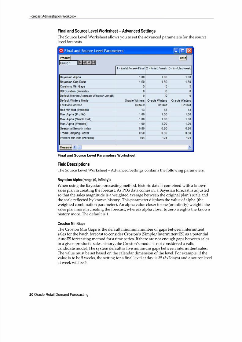
Final and Source Level Worksheet – Advanced SettingsThe Source Level Worksheet allows you to set the advanced parameters for the sourcelevel forecasts.
Final and Source Level Parameters Worksheet
Field DescriptionsThe Source Level Worksheet – Advanced Settings contains the following parameters:
Bayesian Alpha (range (0, infinity))When using the Bayesian forecasting method, historic data is combined with a knownsales plan in creating the forecast. As POS data comes in, a Bayesian forecast is adjustedso that the sales magnitude is a weighted average between the original plan’s scale andthe scale reflected by known history. This parameter displays the value of alpha (theweighted combination parameter). An alpha value closer to one (or infinity) weights thesales plan more in creating the forecast, whereas alpha closer to zero weights the knownhistory more. The default is 1.
Croston Min GapsThe Croston Min Gaps is the default minimum number of gaps between intermittentsales for the batch forecast to consider Croston’s (Simple/IntermittentES) as a potential
AutoES forecasting method for a time series. If there are not enough gaps between salesin a given product’s sales history, the Croston’s model is not considered a validcandidate model. The system default is five minimum gaps between intermittent sales.The value must be set based on the calendar dimension of the level. For example, if thevalue is to be 5 weeks, the setting for a final level at day is 35 (5x7days) and a source levelat week will be 5.
8/10/2019 RDF User Guide
http://slidepdf.com/reader/full/rdf-user-guide 31/120
Forecast Administration Workbook
Setting Forecast Parameters 21
DD Duration (weeks)Used with Profile Based forecast method, the DD Duration is the number of weeks ofhistory required after which the system stops using the DD (De-seasonalized Demand)approach and defaults to the “normal” Profile-Based method. The value must be set
based on the calendar dimension of the level. For example, if the value is to be 10 weeks,the setting for a final level at day is 70 (10x7days) and a source level at week will be 10.
Default Moving Average Window LengthUsed with Moving Average forecast method, this is the Default number of data points inhistory used in the calculation of Moving Average. This parameter can be overwritten atItem/Loc from the Forecast Maintenance Workbook.
Fallback MethodSet this parameter ONLY IF the “Fallback Method” is to vary from the default FallbackMethods used by the selected forecasting algorithm. If the method selected as theDefault Forecast Method or Forecast Method Override does not succeed for a timeseries, this method will be used to calculate the forecast and the default Fallback Methodsin the forecasting process will be skipped entirely. The default Fallback Methods are as
follows: If either the Causal, Bayesian , or Profile-Based are selected as the Default Forecast
Method or Forecast Method Override and the method does not fit the data:Step 1: RDF will attempt to fit SeasonalESStep 2: RDF will attempt to fit TrendESStep 3: RDF will attempt to fit Simple/IntermittentES
If the SeasonalES is selected as the Default Forecast Method or Forecast MethodOverride and neither Multiplicative Seasonal or Additive Seasonal fits the data:Step 1: RDF will attempt to fit TrendESStep 2: RDF will attempt to fit Simple/IntermittentES
If either the Multiplicative Seasonal or Additive Seasonal are selected as theDefault Forecast Method or Forecast Method Override and the method does not fitthe data:Step 1: RDF will attempt to fit TrendESStep 2: RDF will attempt to fit Simple/IntermittentES
If the TrendES is selected as the Default Forecast Method or Forecast MethodOverride and the method does not fit the data:Step 1: RDF will attempt to fit Simple/IntermittentES
Holt Min Hist (Periods)Used with the AutoES forecast method, Holt Min Hist is the minimum number ofperiods of historical data necessary for the system to consider Holt (TrendES) as a
potential forecasting method. Oracle Retail Demand Forecasting fits the given data to avariety of AutoES candidate models in an attempt to determine the best method; if notenough periods of data are available for a given item, Holt will not be considered as avalid option. The system default is 13 periods. The value must be set based on thecalendar dimension of the level. For example, if the value is to be 13 weeks, the setting fora final level at day is 91 (13x7days) and a source level at week will be 13.
8/10/2019 RDF User Guide
http://slidepdf.com/reader/full/rdf-user-guide 32/120
Forecast Administration Workbook
22 Oracle Retail Demand Forecasting
Max Alpha (Profile) (range (0,1])In the Profile-based model fitting procedure, alpha, which is a model parametercapturing the level, is determined by optimizing the fit over the de-seasonalized timeseries. The time series is de-seasonalized based on a seasonal profile. This field displaysthe maximum value (that is, cap value) of alpha allowed in the model fitting process. Analpha cap value closer to 1 allows more reactive models (alpha = 1, repeats the last datapoint), whereas alpha cap closer to 0 only allows less reactive models. The default is 1.
Max Alpha (Simple, Holt) (range (0,1])In the Simple or Holt (TrendES) model fitting procedure, alpha (a model parametercapturing the level) is determined by optimizing the fit over the time series. This fielddisplays the maximum value (cap value) of alpha allowed in the model fitting process.An alpha cap value closer to 1 allows more reactive models (alpha = 1, repeats the lastdata point), whereas alpha cap closer to 0 only allows less reactive models. The default is1.
Max Alpha (Winters) (range (0,1])In the Winters (SeasonalES) model fitting procedure, alpha (a model parameter capturing
the level) is determined by optimizing the fit over the time series. This field displays themaximum value (cap value) of alpha allowed in the model fitting process. An alpha capvalue closer to 1 allows more reactive models (alpha = 1, repeats the last data point),whereas alpha cap closer to 0 only allows less reactive models. The default is 1.
Seasonal Smooth IndexThis parameter is used in the calculation of seasonal index. The current default valueused within forecasting is .80. Changes to this parameter will impact the value ofseasonal index directly and impact the level indirectly. When seasonal smooth index isset to 1, seasonal index will be closer to the seasonal index of last year sales. Whenseasonal smooth index is set to 0, seasonal index will be set to the initial seasonal indexescalculated from history. This parameter is used when the Winters Mode is set to OracleWinters. If the Winters Mode is Winters Standard, Winters Responsive, or Oracle wintersDecomposition, this parameter is optimized and the user input value is ignored.
Trend Damping Factor (range (0,1])This parameter determines how reactive the forecast is to trending data. A value close to0 is a high damping, while a value if 1 implies no damping. The default is 0.5.
Winters Min Hist (Periods)Used with the AutoES forecast method, the value in this field is the minimum number ofperiods of historical data necessary for Winters to be considered as a potential forecastmethod. If not enough years of data are available for a given time series, Winters will not
be used. The system default is two years of required history. The value must be set basedon the calendar dimension of the level. For example, if the value is to be 104 weeks/2years, the setting for a final level at day is 728 (104 weeks x 7 days) and a source level atweek will be 104.
8/10/2019 RDF User Guide
http://slidepdf.com/reader/full/rdf-user-guide 33/120
Forecast Administration Workbook
Setting Forecast Parameters 23
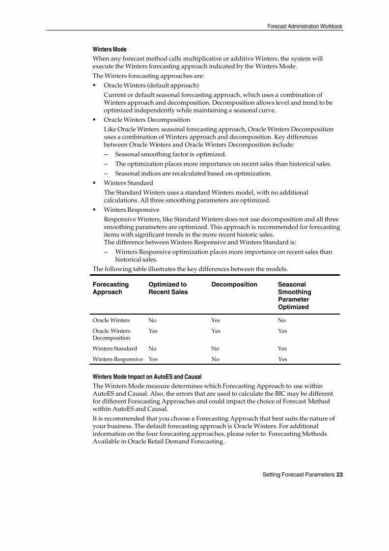
Winters ModeWhen any forecast method calls multiplicative or additive Winters, the system willexecute the Winters forecasting approach indicated by the Winters Mode.The Winters forecasting approaches are: Oracle Winters (default approach)
Current or default seasonal forecasting approach, which uses a combination ofWinters approach and decomposition. Decomposition allows level and trend to beoptimized independently while maintaining a seasonal curve.
Oracle Winters DecompositionLike Oracle Winters seasonal forecasting approach, Oracle Winters Decompositionuses a combination of Winters approach and decomposition. Key differences
between Oracle Winters and Oracle Winters Decomposition include: – Seasonal smoothing factor is optimized. – The optimization places more importance on recent sales than historical sales. – Seasonal indices are recalculated based on optimization.
Winters Standard
The Standard Winters uses a standard Winters model, with no additionalcalculations. All three smoothing parameters are optimized.
Winters ResponsiveResponsive Winters, like Standard Winters does not use decomposition and all threesmoothing parameters are optimized. This approach is recommended for forecastingitems with significant trends in the more recent historic sales.The difference between Winters Responsive and Winters Standard is:
– Winters Responsive optimization places more importance on recent sales thanhistorical sales.
The following table illustrates the key differences between the models.
ForecastingApproach
Optimized toRecent Sales
Decomposition SeasonalSmoothingParameterOptimized
Oracle Winters No Yes No
Oracle WintersDecomposition
Yes Yes Yes
Winters Standard No No Yes
Winters Responsive Yes No Yes
Winters Mode Impact on AutoES and Causal
The Winters Mode measure determines which Forecasting Approach to use withinAutoES and Causal. Also, the errors that are used to calculate the BIC may be differentfor different Forecasting Approaches and could impact the choice of Forecast Methodwithin AutoES and Causal.It is recommended that you choose a Forecasting Approach that best suits the nature ofyour business. The default forecasting approach is Oracle Winters. For additionalinformation on the four forecasting approaches, please refer to Forecasting MethodsAvailable in Oracle Retail Demand Forecasting .
8/10/2019 RDF User Guide
http://slidepdf.com/reader/full/rdf-user-guide 34/120
Forecast Administration Workbook
24 Oracle Retail Demand Forecasting
Note: If patching this change into a domain, in order to viewthis measure in the Forecast Administration workbook, itmust be added to the Final and Source Level Parameters worksheet by selecting it from the Show/Hide dialog withinthe RPAS Client.
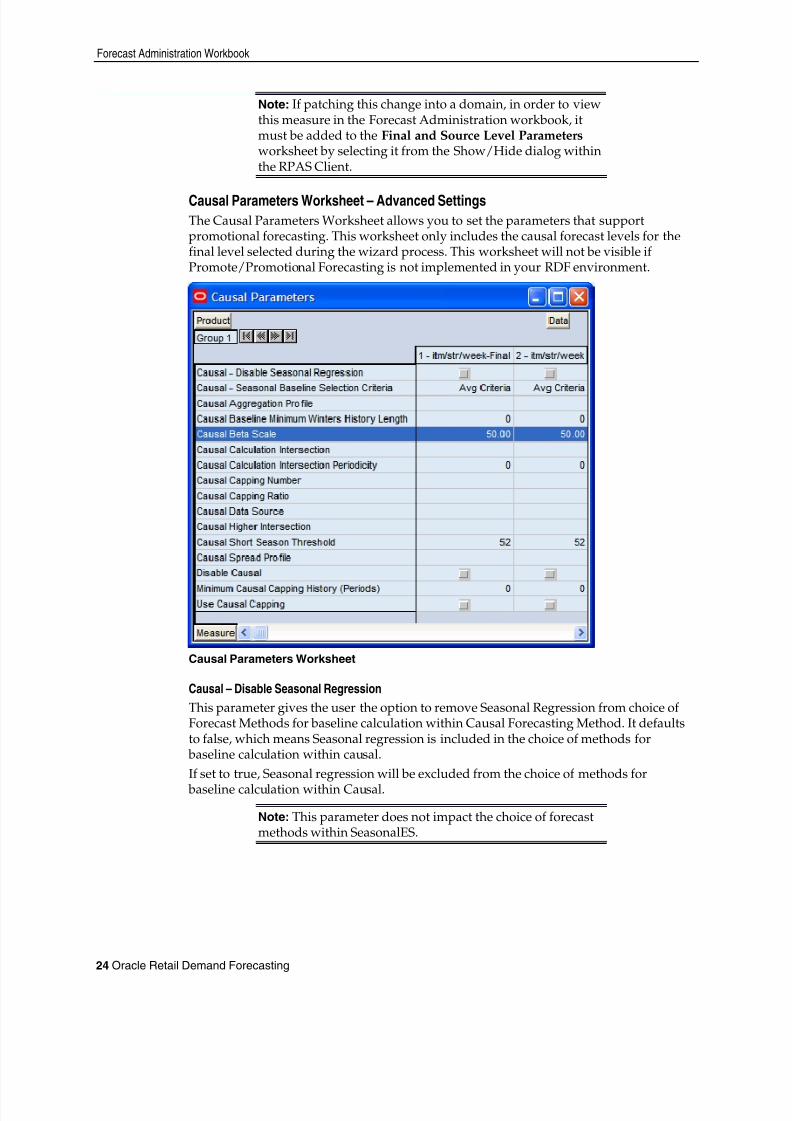
Causal Parameters Worksheet – Advanced SettingsThe Causal Parameters Worksheet allows you to set the parameters that supportpromotional forecasting. This worksheet only includes the causal forecast levels for thefinal level selected during the wizard process. This worksheet will not be visible ifPromote/Promotional Forecasting is not implemented in your RDF environment.
Causal Parameters Worksheet
Causal – Disable Seasonal RegressionThis parameter gives the user the option to remove Seasonal Regression from choice ofForecast Methods for baseline calculation within Causal Forecasting Method. It defaultsto false, which means Seasonal regression is included in the choice of methods for
baseline calculation within causal.If set to true, Seasonal regression will be excluded from the choice of methods for
baseline calculation within Causal.
Note: This parameter does not impact the choice of forecastmethods within SeasonalES.
8/10/2019 RDF User Guide
http://slidepdf.com/reader/full/rdf-user-guide 35/120
Forecast Administration Workbook
Setting Forecast Parameters 25
Causal – Seasonal Baseline Selection CriteriaThis parameter allows the user to choose whether to use minimum or average baselinecriteria to determine baseline stability within Causal Forecasting Method. Average baseline criteria: If system calculated average baseline forecast < 4, use Beta
zero as System baseline forecast.
Minimum baseline criteria: If system calculated minimum baseline forecast < 1, thenuse Beta zero as System baseline forecast.This parameter defaults to Average Baseline Criteria.
Causal Aggregation ProfileUsed only for Daily Causal Forecasting, the Causal Aggregation Profile is measure nameof the profile used to aggregate promotions defined at “day” up to the “week.” The valueentered in this field is the measure name of profile. If this profile is generated withinCurve, the format of the measure name will be “apvp”+level (for example: apvp01). Notethat the only aggregation of promotion variables being performed here is along theCalendar hierarchy. RDF does not support aggregation of promotion variables alongother hierarchies such as product and location hierarchies.
Causal Beta ScaleAs part of the causal forecasting process, the average sales of non-promo periods inhistory are divided by the Beta Scale. If the betazero is above the Causal Beta Scale value, the causal forecasting method succeeds. If not, the causal forecasting method failsand the Fallback Method is used to generate the forecast for the time series.
Causal Calculation IntersectionUsed only for Daily Causal Forecasting, the Causal Calculation Intersection is theintersection at which the causal forecast is run. The format needs to match the hierarchydimension names set in the RPAS Configuration Tools (such as “itemstr_week”). Eachdimension must have only four characters. The order of the dimension does not matter.There is no validation of correct format of this intersection.
Causal Calculation Intersection PeriodicityUsed only for Daily Causal Forecasting, the Causal Calculation Intersection Periodicitymust be set to the periodicity of Causal Calculation Intersection. Periodicity is thenumber of periods within one year that correspond to the calendar dimension (forexample, 52 if the Causal Calculation Intersection is defined with the week dimension).
Causal Capping NumberThe value of this parameter is a measure based on the same product and locationintersection as the forecast level. This measure contains the maximum value to use forcalculating the causal forecast for time series that meet the Causal Capping conditions. IfUse Causal Capping is set to true, the history for the time series is greater than or equalto the Minimum Causal Capping History , and the preliminary forecast is greater than orequal to the value in the Causal Capping Number measure, then the forecast will berecalculated to be the value in the Causal Capping Number measure multiplied by thevalue in the Causal Capping Ratio measure.
8/10/2019 RDF User Guide
http://slidepdf.com/reader/full/rdf-user-guide 36/120
Forecast Administration Workbook
26 Oracle Retail Demand Forecasting
Causal Capping RatioThe value of this parameter is a measure based on the same product and locationintersection as the forecast level. This measure contains the ratio to be used to calculatethe forecasts for time series that meet the Causal Capping conditions. If Use CausalCappin g is set to true, the history for the time series is greater than or equal to the valuein the Minimum Causal Capping History measure, and the preliminary forecast isgreater than or equal to the value in the Causal Capping Number measure, then theforecast will be recalculated to be the Causal Capping Number multiplied by the valuein the Causal Capping Ratio measure.
Causal Data SourceUsed only for Daily Causal Forecasting, the Causal Data Source is an optional setting thatcontains the measure name of the sales data to be used if the data for causal forecasting isdifferent than the Data Source specified at the Final level. If needed, this field shouldcontain the measure name of the source data measure (for example: dpos).
Causal Higher IntersectionAn optional setting for Causal Forecasting, this intersection is the aggregate level to
model promotions if the causal intersection cannot produce a meaningful causal effect.This intersection will apply to promotions that have a Promotion Type is set to OverrideFrom Higher Level (set in the Promotion Maintenance workbook). The format of thisintersection needs to match the hierarchy dimension names set in the RPASConfiguration Tools—such as “sclsrgn_” (Subclass\Region), and it must not contain thecalendar dimension. Each dimension must have only four characters. The order of thedimension does not matter. There is no validation of correct format of this intersection.
Causal Short Seasonal ThresholdUsed only in Causal forecasting, this parameter is the minimum number of historicaltime periods that are required for SeasonalES to be used to produce the Causal forecast.Otherwise, the baseline from Causal regression will be used. The algorithm currentlyuses 52 weeks of history as the default for this parameter, but it may be set from 13 to 56weeks. For an item with history less than the value in the Causal Short SeasonalThreshold and greater than 12 weeks, the BetaZero will be used only if Causal found theinitial effects to be significant. Otherwise, the item will be forecasted using the FallbackMethod.
Causal Spread ProfileUsed only for Daily Causal Forecasting, the Causal Spread Profile is the measure name ofthe profile used to spread the causal baseline forecast from the Causal CalculationIntersection to the Final Level. If this profile is generated in Curve, this measure valuewill be “apvp”+level (for example: apvp01).
Minimum Causal Capping History (Periods)
If Use Causal Capping is set to true, this parameter is used to set minimum number ofhistorical time periods required before the system will consider a time series for causalcapping.
Disable CausalPlace a check in this parameter (set to true) if causal forecasting is to be disabled for theforecast level. This parameter serves as a global override. This parameter can also helpwith performance, when not running Causal forecast method.
8/10/2019 RDF User Guide
http://slidepdf.com/reader/full/rdf-user-guide 37/120
Forecast Maintenance Workbook
Setting Forecast Parameters 27
Use Causal CappingPlace a check in this parameter (set to true) if capping is to be applied to the causalforecast. Also required for causal capping are the following parameters: Causal Capping Number Causal Capping Ratio
Minimum Causal Capping HistoryNote: More detailed information on the Causal forecastingalgorithm is provided in “ Forecasting Methods Available inOracle Retail Demand Forecasting .”
Forecast Maintenance Workbook
OverviewThe Forecast Maintenance Workbook allows you to select and modify forecastingparameters for product/location combinations when the values of these parametersdiffer from the default values that are assigned in the Forecast AdministrationWorkbook.Suppose, for example, that the default forecast method of all the products in the databasewas set in the Forecast Administration Workbook to be AutoES. For a particular product,however, you know that a SeasonalES model is a better predictor of sales performance.To make this change, you must access the Forecast Maintenance Workbook, select theproduct / location intersection to be reviewed, and make the appropriate change to theforecast method.The Forecast Maintenance Workbook is split into two workflow tabs: Basic Settings – Includes all Final Level Worksheets and their respective Source Level
Worksheets. Advanced Settings –This tab includes the Forecast Start Date, End Date. and History
Start Date measures for the selected Final Level.
Creating a Forecast Maintenance Workbook1. Within the Master or Local Domain, select New from the File menu.2. Select the Forecast tab to display a list of workbook templates for statistical
forecasting. Highlight Forecast Maintenance.3. Click OK . The Forecast Maintenance wizard opens and prompts you to select the
level of the final forecast. Depending on your organization's setup, you may beoffered a choice of several final forecast levels.
4. Select the final forecast level to be viewed in the workbook.5. Click Next .
6. Select the locations to include in the workbook.7. Click Next .8. Select the products to include in the workbook.9. Click Next .10. Select any additional measures (that is, measures not standard in the Forecast
Maintenance Workbook) that you would like included. The measure optionsavailable in this screen are set in the RPAS Security Administration Workbook /Workbook Template Measure Rights Worksheet.
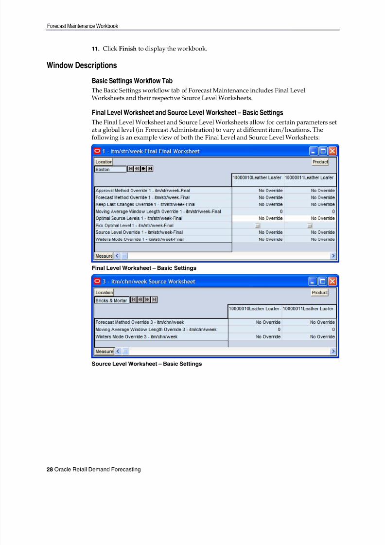
8/10/2019 RDF User Guide
http://slidepdf.com/reader/full/rdf-user-guide 38/120
Forecast Maintenance Workbook
28 Oracle Retail Demand Forecasting
11. Click Finish to display the workbook.
Window Descriptions
Basic Settings Workflow TabThe Basic Settings workflow tab of Forecast Maintenance includes Final LevelWorksheets and their respective Source Level Worksheets.
Final Level Worksheet and Source Level Worksheet – Basic SettingsThe Final Level Worksheet and Source Level Worksheets allow for certain parameters setat a global level (in Forecast Administration) to vary at different item/locations. Thefollowing is an example view of both the Final Level and Source Level Worksheets:
Final Level Worksheet – Basic Settings
Source Level Worksheet – Basic Settings
8/10/2019 RDF User Guide
http://slidepdf.com/reader/full/rdf-user-guide 39/120
Forecast Maintenance Workbook
Setting Forecast Parameters 29
Field DescriptionsThe Final Level Worksheet and Source Level Worksheet – Basic Settings contains thefollowing parameters:
Approval Method OverrideSet only at the final level, the Approval Method Override is a drop-down list from whichyou select the approval policy for individual product/location combinations. No valuewill be in this field if the system default set in the Forecast Administration Workbook isto be used. Valid values are: Manual – The System Forecast and Adjusted Forecast are not automatically
approved. Forecast values must be manually approved by accessing and amendingthe Forecast Approval Workbook.
Automatic – The Adjusted Forecast is automatically approved as-is. By alert “name of the alert” – This list of values may also include any Forecast
Approval alerts that have been configured for use in the forecast approval process.Alerts are configured during the implementation. See the RPAS Configuration ToolsUser Guide for more information on the Alert Manager, and the RDF Configuration
Guide for more information on configuring Forecast Approval Alerts.Note: If you select a specific alert as your approval methodand later on you delete the alert, the approval will work asmanual. The same will happen if the alert is on a wrongintersection.
Forecast Method OverrideSet at both final and source levels, the Forecast Method Override is a drop-down list fromwhich you can select a different forecast method than the Default Forecast Method set inthe Forecast Administration workbook. No Override appears in this field if the systemdefault set in the Forecast Administration Workbook is to be used. Valid options dependon your system setup.
Winters Mode OverrideUsed only by Forecasting Methods calling Additive or Multiplicative Winters. Thisparameter allows the user to override the Winters Mode setting assigned in the ForecastAdministration workbook. The default setting for this parameter is No Override.
Keep Last Changes OverrideSet only at final levels, Keep Last Changes Override field may be used to override thedefault setting at a product/location intersection. None appears in this field if there is nooverride applied to the intersection.
Optimal Source Levels
Displayed only at final levels, a value will be populated in this field if AutoSource has been run on the final level. The AutoSource executable evaluates all levels associated to afinal level and returns the source level that yields the optimal forecast results. For moreinformation on AutoSource, see the RDF Administration Guide .
Pick Optimal LevelSet only at final levels, a check in this field (set to true) indicates that the batch forecastshould use the Optimal Source Level selected by AutoSource. For more information onAutoSource, see the RDF Administration Guide .
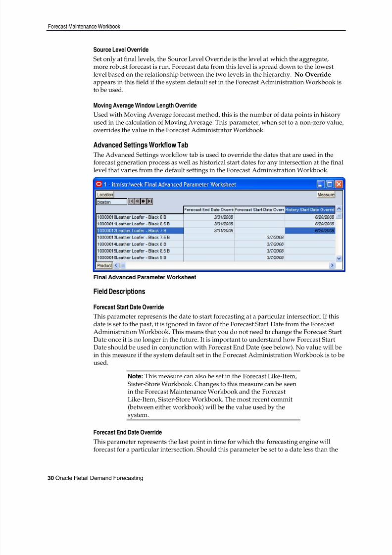
8/10/2019 RDF User Guide
http://slidepdf.com/reader/full/rdf-user-guide 40/120
Forecast Maintenance Workbook
30 Oracle Retail Demand Forecasting
Source Level OverrideSet only at final levels, the Source Level Override is the level at which the aggregate,more robust forecast is run. Forecast data from this level is spread down to the lowestlevel based on the relationship between the two levels in the hierarchy. No Override appears in this field if the system default set in the Forecast Administration Workbook isto be used.
Moving Average Window Length OverrideUsed with Moving Average forecast method, this is the number of data points in historyused in the calculation of Moving Average. This parameter, when set to a non-zero value,overrides the value in the Forecast Administrator Workbook.
Advanced Settings Workflow TabThe Advanced Settings workflow tab is used to override the dates that are used in theforecast generation process as well as historical start dates for any intersection at the finallevel that varies from the default settings in the Forecast Administration Workbook.
Final Advanced Parameter Worksheet
Field Descriptions
Forecast Start Date OverrideThis parameter represents the date to start forecasting at a particular intersection. If thisdate is set to the past, it is ignored in favor of the Forecast Start Date from the ForecastAdministration Workbook. This means that you do not need to change the Forecast StartDate once it is no longer in the future. It is important to understand how Forecast StartDate should be used in conjunction with Forecast End Date (see below). No value will bein this measure if the system default set in the Forecast Administration Workbook is to beused.
Note: This measure can also be set in the Forecast Like-Item,Sister-Store Workbook. Changes to this measure can be seenin the Forecast Maintenance Workbook and the ForecastLike-Item, Sister-Store Workbook. The most recent commit(between either workbook) will be the value used by thesystem.
Forecast End Date OverrideThis parameter represents the last point in time for which the forecasting engine willforecast for a particular intersection. Should this parameter be set to a date less than the

8/10/2019 RDF User Guide
http://slidepdf.com/reader/full/rdf-user-guide 41/120
Forecast Like-Item, Sister-Store Workbook
Setting Forecast Parameters 31
Forecast Start Date plus the Forecast Length (in Forecast Administration), the engine willforecast 0 past this date. If Forecast End Date is more than Forecasting Start Date plusForecasting Length, you do NOT get a forecast outside Forecasting Start Date plusForecasting Length. In other words, both Forecast Start Date and Forecasting End Dateare relevant for time periods within the forecast horizon set at the global level. No valuewill be in this measure if the system default set in the Forecast Administration Workbook
is to be used.Note: This measure can also be set in the Forecast Like-Item,Sister-Store Workbook. Changes to this measure can be seenin the Forecast Maintenance Workbook and the ForecastLike-Item, Sister-Store Workbook. The most recent commit(in either workbook) will be the value used by the system.
History Start Date OverrideThis parameter represents the first point in time from which the Forecasting Engine will
begin training and modeling (that is, if there are two years of history, but you only wantto use one year, you will set the start date to a year ago). This parameter will override theHistory Start Date set in the Forecast Administration Workbook to the desireditem/location intersection. For example, if you have a large spike in the first three weeksof sales for an item was on sale, you can set the Historical Start Date to one week pastthat period, and those first few weeks will not be used when generating the forecast.It is also important to note that the system ignores leading zeros that begin at the historystart date. For example, if your history start date is January 1, 2003 and an item/locationdoes not have sales history until February 1, 2003, the system will consider the startingpoint in that item/location’s history to be the first data point where there is a non-zerosales value.If this parameter is set into the future, there would be no forecast as the history trainingwindow is read as zero.
Note: This measure can also be set in the Forecast Like-Item,Sister-Store Workbook. Changes to this measure can be seenin the Forecast Maintenance Workbook and the ForecastLike-Item, Sister-Store Workbook. The most recent commit(between either workbook) will be the value used by thesystem.
Forecast Like-Item, Sister-Store Workbook
OverviewThe Forecast Like-Item, Sister-Store Workbook provides the ability to model a newproduct’s demand after an existing product. Forecasts can thus be generated for the new
product based on the selected history or the forecast of the existing product plus anAdjustment Ratio. Likewise, the sales history or the forecast of existing store locationscan be used as the forecast foundation for new locations. This workbook includes thefollowing worksheets: The Like-Item Worksheet The Sister-Store Worksheet The Advanced Parameter Worksheet
8/10/2019 RDF User Guide
http://slidepdf.com/reader/full/rdf-user-guide 42/120
Forecast Like-Item, Sister-Store Workbook
32 Oracle Retail Demand Forecasting
Note: This workbook is only valid at final levels. Therefore,this workbook may include hierarchy dimensions that are athigher positions that item or store (for example: subclass orregion).
Creating a Forecast Like-Item, Sister-Store Workbook1. Within the Simple or Local Domain, select New from the File menu.2. Select the Forecast tab to display a list of workbook templates for statistical
forecasting. Highlight Forecast Like-Item, Sister-Store .3. Click OK . The wizard opens and prompts you to select the level of the final forecast.
Depending on your organization's setup, you may be offered a choice of several finalforecast levels.
4. Select the final forecast level to be viewed in the workbook.5. Click Next .6. Select the locations to include in the workbook.7. Click Next .
8. Select the products to include in the workbook.9. Click Next .10. Select any additional measures (that is, measures not standard in the Forecast Like-
Item, Sister-Store Workbook) to be included. The measure options available in thisscreen are set in the RPAS Security Administration Workbook / Workbook TemplateMeasure Rights Worksheet.
11. Click Finish to display the workbook.
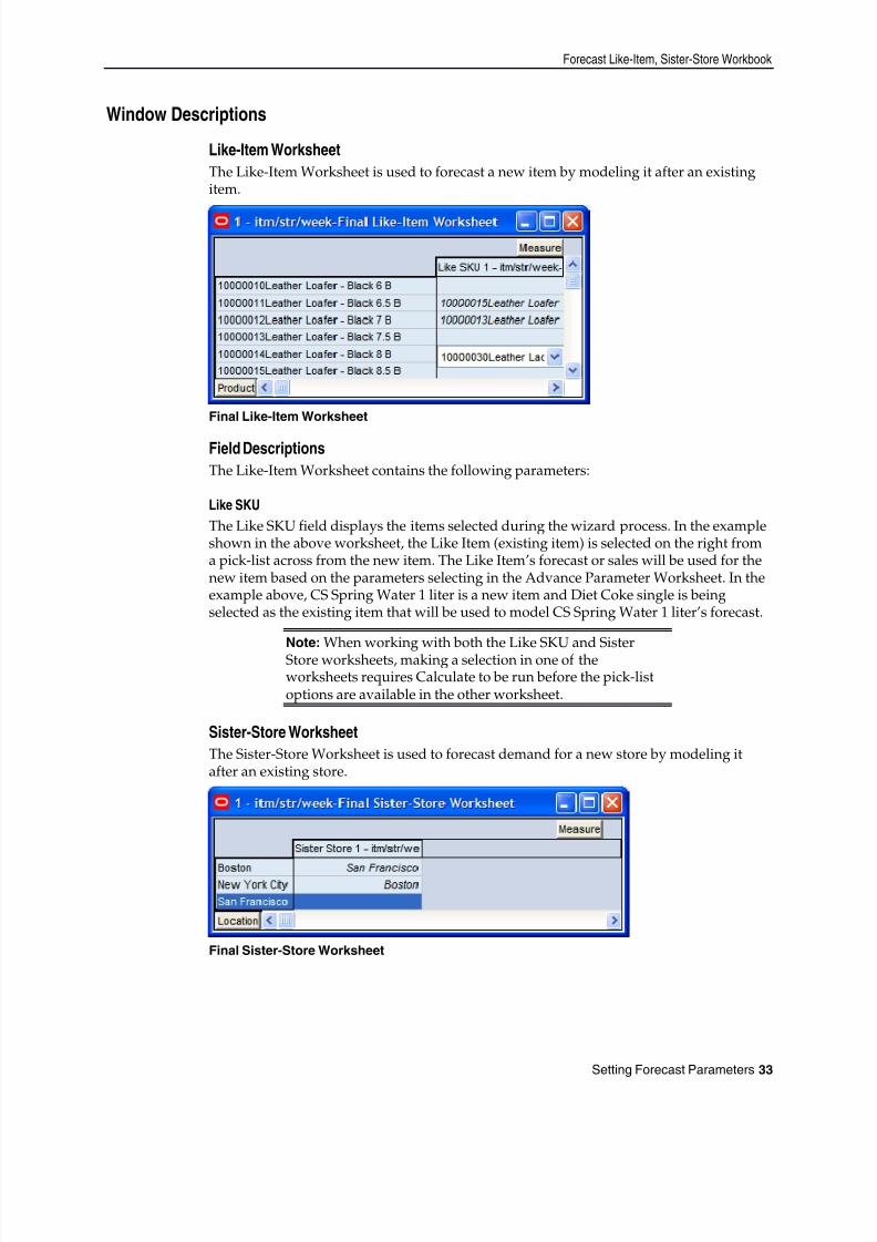
8/10/2019 RDF User Guide
http://slidepdf.com/reader/full/rdf-user-guide 43/120
Forecast Like-Item, Sister-Store Workbook
Setting Forecast Parameters 33
Window Descriptions
Like-Item WorksheetThe Like-Item Worksheet is used to forecast a new item by modeling it after an existingitem.
Final Like-Item Worksheet
Field DescriptionsThe Like-Item Worksheet contains the following parameters:
Like SKUThe Like SKU field displays the items selected during the wizard process. In the exampleshown in the above worksheet, the Like Item (existing item) is selected on the right froma pick-list across from the new item. The Like Item’s forecast or sales will be used for thenew item based on the parameters selecting in the Advance Parameter Worksheet. In theexample above, CS Spring Water 1 liter is a new item and Diet Coke single is beingselected as the existing item that will be used to model CS Spring Water 1 liter’s forecast.
Note: When working with both the Like SKU and SisterStore worksheets, making a selection in one of theworksheets requires Calculate to be run before the pick-listoptions are available in the other worksheet.
Sister-Store WorksheetThe Sister-Store Worksheet is used to forecast demand for a new store by modeling itafter an existing store.
Final Sister-Store Worksheet

8/10/2019 RDF User Guide
http://slidepdf.com/reader/full/rdf-user-guide 44/120
Forecast Like-Item, Sister-Store Workbook
34 Oracle Retail Demand Forecasting
Field DescriptionsThe Sister-Store Worksheet contains the following parameter:
Sister StoreDisplays the locations selected during the wizard process. In the example shown in theabove worksheet, the Sister Store (existing Store) is selected on the right from a pick-listacross from the new Store. The Sister Store’s forecast or sales will be used for the newStore based on the parameters selecting in the Advance Parameter Worksheet. In thescreen shot above, the Boston is the new store and San Francisco is being selected as thestore to be used for modeling Boston’s forecast.
Note: When working with both the Like SKU and SisterStore worksheets, if a selection is made in one of theworksheets, Calculate must be run before the pick-listoptions are available in the other worksheet.
Advance Parameter WorksheetThe Advance Parameter Worksheet is used to manage item/locations in which theForecast Start Date, Forecast End Date, or History Start Date varies from the defaultsettings in the Forecast Administration Workbook and to set the Adjustment Ratio for thenew item or location being forecasted.
Final Advanced Parameter Worksheet
Field DescriptionsThe Advanced Parameter Worksheet contains the following parameters:
Adjustment RatioThe user may enter an Adjustment Ratio to apply to the forecast for the new product /location combination displayed. This is a real number between [0, ∞) . The default (NA)value is 1.00, (in other words 100%) which translates to no adjustment.
Example: If demand for a new item is expected to be 30%greater than its like item, the Adjustment Ratio would be setto 1.30. If demand for a new item is expected to be 30% lessthan its Like Item, the Adjustment % would set to .70.

8/10/2019 RDF User Guide
http://slidepdf.com/reader/full/rdf-user-guide 45/120
Forecast Like-Item, Sister-Store Workbook
Setting Forecast Parameters 35
Forecast Start Date OverrideThis parameter represents the date to start forecasting for an item/location combination.This parameter can be set in the future if using Like Item or Sister Store functionality andupon reaching that time, the forecast will be generated. If this date is set to the past, it isignored in favor of the Forecast Start Date from the Forecast Administration Workbook.This means that the Forecast Start Date for this intersection needs to be edited once it isno longer in the future. For Like item or Sister Store, the Forecast Start Date and theHistory Start Date should be set to the same date. It is important to understand howForecast Start Date should be used in conjunction with Forecast End Date (See below).No value will be in this measure if the system default set in the Forecast AdministrationWorkbook is to be used.
Note: This measure can also be set in the ForecastMaintenance Workbook. Changes to this measure can beseen in the Forecast Maintenance Workbook and theForecast Like-Item, Sister-Store Workbook. The most recentcommit (between either of the workbooks) will be the valueused by the system.
Forecast End Date OverrideThis parameter represents the last point in time for which the Forecasting Engine willforecast for an item/location combination. Should this parameter be set to a date lessthan the Forecast Start Date plus the Forecast Length (in Forecast Administration), theengine will forecast 0 past this date. If Forecast End Date is more than Forecasting StartDate plus Forecasting Length, NO forecast will be generated outside Forecasting StartDate plus Forecasting Length window. In other words, both Forecast Start Date andForecasting End Date are relevant for time periods within the forecast horizon set at theglobal level. No value will be in this measure if the system default set in the ForecastAdministration Workbook is to be used.Forecast End Date can be used for new item or location forecasting if the item or locationneeds to be forecasted for a period shorter than the Like TS Duration (set globally inForecast Administration).
Note: This measure can also be set in the ForecastMaintenance Workbook. Changes to this measure can beseen in the Forecast Maintenance Workbook and theForecast Like-Item, Sister-Store Workbook. The most recentcommit (between either of the workbooks) will be the valueused by the system.
History Start Date OverrideThis parameter represents the first point in time from which the Forecasting Engine will
begin training and modeling (that is, if there are two years of history, but only one year is
required, set the start date to a year ago). This parameter overrides at the item/store levelfrom the global settings in the Forecast Administration Workbook. This can be used tolevel out past sales. For example, if there is a large spike in the first three weeks of salesfor an item was on sale, set the Historical Start Date to one week past that period, andthose first few weeks will not be used when generating the forecast.
8/10/2019 RDF User Guide
http://slidepdf.com/reader/full/rdf-user-guide 46/120
Forecast Like-Item, Sister-Store Workbook
36 Oracle Retail Demand Forecasting
It is also important to note that the system ignores leading zeros that begin at the historystart date. For example, if your history start date is January 1, 1999 and an item/locationdoes not have sales history until February 1, 1999, the system will consider the startingpoint in that item/location’s history to be the first data point where there is a non-zerosales value.The History Start Date for the new item or new store should be set with the same date asthe Forecast Start Date.
Note: When using any of the Lifecycle Methods (seeSubstitute Methods below), the History Start Date for thesubstitute item or location must be set to the point in thesales history that the new item or location will begin using asits sales.
Note: This measure can also be set in the ForecastMaintenance Workbook. Changes to this measure can beseen in the Forecast Maintenance Workbook and theForecast Like-Item, Sister-Store Workbook. The most recentcommit (between either of the workbooks) will be the value
used by the system.
Substitute MethodDisplays a drop-down list from which the user can select the substitute method. When aSubstitute Method is used to forecast, the method set for an intersection will be clearedonce the Default Forecast Start Date is greater than the Forecast Start Date Override plusthe Like TS Duration for the intersection. Valid options are: None – There is no substitution for this product/location combination. This is the
default value. Seasonality/New Item – The user provides a Like Item that has a similar seasonality
pattern that sells at the same store. The new product’s forecast will be the like item’sdemand forecast with the applied adjustment. The forecast will be set to 0 for alldates before the new product’s start date.
Seasonality/New Store – The user provides a Sister Store that has a similarseasonality pattern that sells the same product. The product’s forecast at the newstore will be the demand forecast of the same product at the Sister Store with theapplied adjustment. The forecast will be set to 0 for all dates before the new store’sopen date.
Seasonality/New Item /New Store – The user provides a Like Item that sells at aSister Store that has a similar seasonality pattern. The new product’s forecast at thenew store will be the demand forecast of the Like Item at the Sister Store with theapplied adjustment. The forecast will be set to 0 for all dates before the new product’sstart date after the new store opens.
Lifecycle/New Item – The user provides a Like Item that had a similar lifecyclepattern that sells at the same store. The new product’s forecast will be the like itemsactual sales with the applied adjustment shifted such that the like item’s first salesmatches the new product’s start date.
Lifecycle/New Store – The user provides a Sister Store that had a similar lifecyclepattern that sells the same product. The product’s forecast at the new store will bethe products actual sales at the Sister Store with the applied adjustment shifted suchthat the Sister Store’s first sales matches the new store’s open date.
8/10/2019 RDF User Guide
http://slidepdf.com/reader/full/rdf-user-guide 47/120
Forecast Like-Item, Sister-Store Workbook
Setting Forecast Parameters 37
Lifecycle/New Item /New Store – The user provides a Like Item that sells at a SisterStore that has a similar lifecycle pattern. The new product’s forecast at the new storewill be Like Item’s actual sales at a Sister Store with the applied adjustment shiftedsuch that the Like Item’s first sales at the Sister Store matches the new product’s startdate after the new store opens.
Steps Required for Forecasting Using Each of the Like SKU / Sister Store MethodsThe following outlines the steps required for using each of the above SubstitutionMethods:To support Like SKU / Sister Store functionality, the Like TS Duration must be set in theForecast Administration Workbook – Advance Tab. This parameter sets the number ofweeks of history required after which Oracle Retail Demand Forecasting stops using thesubstitution method and starts using the system forecast generated by the forecastengine.
Procedures
Seasonality/SKU: Introduction of a new item at an existing store (like item with a similar forecast)
1. Like-Item Worksheet ─ Select a like item from the drop-down list across from thenew item.
2. Advanced Parameter Worksheet ─ Set the Forecast Start Date for the new item at anexisting store.
3. Advanced Parameter Worksheet ─ Set the History Start Date for the new item at theexisting store to the same date as the Forecast Start Date.
4. Advance Parameter Worksheet ─ Set the Adjustment % (optional) for the new itemat the existing store.
Seasonality/STR: Introduction of an existing item at a new store (sister store with similar forecast)1. Sister-Store Worksheet ─ Select a Sister Store from the drop-down list, across from
the new store.2. Advanced Parameter Worksheet ─ Set the Forecast Start Date for the existing item atthe new store.
3. Advanced Parameter Worksheet ─ Set the History Start Date for the existing item atthe new store to the same date as the Forecast Start Date.
4. Advance Parameter Worksheet ─ Set the Adjustment % (optional) for the existingitem at the new store.
Seasonality/SKU_STR: Introduction of a new item at a new store (like item and sister store with asimilar forecast)1. Like-Item Worksheet ─ Select a like item from the drop-down list across from the
new item.2. Sister-Store Worksheet ─ Select a Sister Store from the drop-down list across from
the new store.3. Advanced Parameter Worksheet ─ Set the Forecast Start Date at the intersection of
the new item and the new store.4. Advanced Parameter Worksheet ─ Set the History Start at the intersection of the
new item and new store.5. Advance Parameter Worksheet ─ Set the Adjustment % (optional) at the intersection
of the new item and new store.
8/10/2019 RDF User Guide
http://slidepdf.com/reader/full/rdf-user-guide 48/120
Forecast Like-Item, Sister-Store Workbook
38 Oracle Retail Demand Forecasting
Lifecycle/SKU - Introduction of a new item at an existing store (Like item’s sales history to be used asthe forecast for the new item)1. Like-Item Worksheet ─ Select a like item from the drop-down list across from the
new item.2. Advanced Parameter Worksheet ─ Set the Forecast Start Date for the new item at the
existing store.3. Advanced Parameter Worksheet ─ Set the History Start Date for the new item at the
existing store to the same date as the Forecast Start Date.4. Advanced Parameter Worksheet ─ Set the History Start Date for the Like item at the
existing store to the point in its sales history that will map to the new item’s forecast.5. Advance Parameter Worksheet ─ Set the Adjustment % (optional) for the new item
at the existing store.
Lifecycle/STR: Introduction of an existing item at new store (Sister Store’s sales history to be usedas the forecast for the new store)1. Sister-Store Worksheet ─ Select a Sister Store from the drop-down list across from
the new Store.
2. Advanced Parameter Worksheet ─ Set the Forecast Start Date for the existing item atthe new store.
3. Advanced Parameter Worksheet ─ Set the History Start Date for the existing item atthe new store to the same date as the Forecast Start Date.
4. Advanced Parameter Worksheet ─ Set the History Start Date at the intersection ofthe Sister Store and existing item to the date in its sales history that will map to thenew store’s forecast.
5. Advance Parameter Worksheet ─ Set the Adjustment % (optional) for the existingitem at the new store.
Lifecycle/SKU_STR: Introduction of a new item at a new store (Like item’s and Sister Store’s saleshistory to be used as the forecast for a new item at a new store)1. Like-Item Worksheet ─ Select a like item from the drop-down list across from the
new item.2. Sister-Store Worksheet ─ Select a Sister Store from the drop-down list across from
the new store.3. Advanced Parameter Worksheet ─ Set the Forecast Start Date at the intersection of
the new item and new store.4. Advanced Parameter Worksheet ─ Set the History Start Date at the intersection of
the new item and new store to the same date as the Forecast Start Date.5. Advanced Parameter Worksheet ─ Set the History Start Date at the intersection of
the Like item and Sister Store to the date in its sales history that will map to the newitem and new store’s forecast.
6. Advance Parameter Worksheet ─ Set the Adjustment % (optional) at the intersectionof the new item and new store
8/10/2019 RDF User Guide
http://slidepdf.com/reader/full/rdf-user-guide 49/120
Product/Location Cloning Administration Workbook
Setting Forecast Parameters 39
Product/Location Cloning Administration Workbook
OverviewThe Product/Location Cloning Administration Workbook allows users to specifyparameters to clone or copy history for new Items or Locations from existing Items and
Locations. Since RDF needs history for forecasting, this functionality allows users tospecify clone items and clone Stores for these new Product/Locations.Cloning is different from Like Item/Sister Store functionality. Like item/Sister storefunctionality copies forecasts or history of the like item or sister store as the forecasts forthe new SKU/Store. However, in cases where the two items have different promotioncalendars, it is necessary to forecast based on history data and promotion calendar.Item/Loc Cloning functionality facilitates this process.Also, by copying history from the parent product, users can start forecasting almostimmediately after the launch of the new product.Product/Location Cloning Administration can be performed from the Master or Localdomain. The actual cloning or copying of history can be performed as part of batch run.
Note: Clone is available as a special expression that can beconfigured to be called as a batch run to perform the actualcopying of history.
Note: When the Cloning administration Workbook is built inthe Master domain, if clone assignments are made such thata product is assigned a clone that belongs to a different localdomain, then at the time of batch run RDF will not clone thatspecific product and continue processing after logging amessage.
This workbook includes the following worksheets: Product Cloning Worksheet
Location Cloning Worksheet Clone Mask Worksheet
Note: This workbook is only valid at final levels. Therefore,this workbook may include hierarchy dimensions that are athigher positions than item or store (for example: subclass orregion).
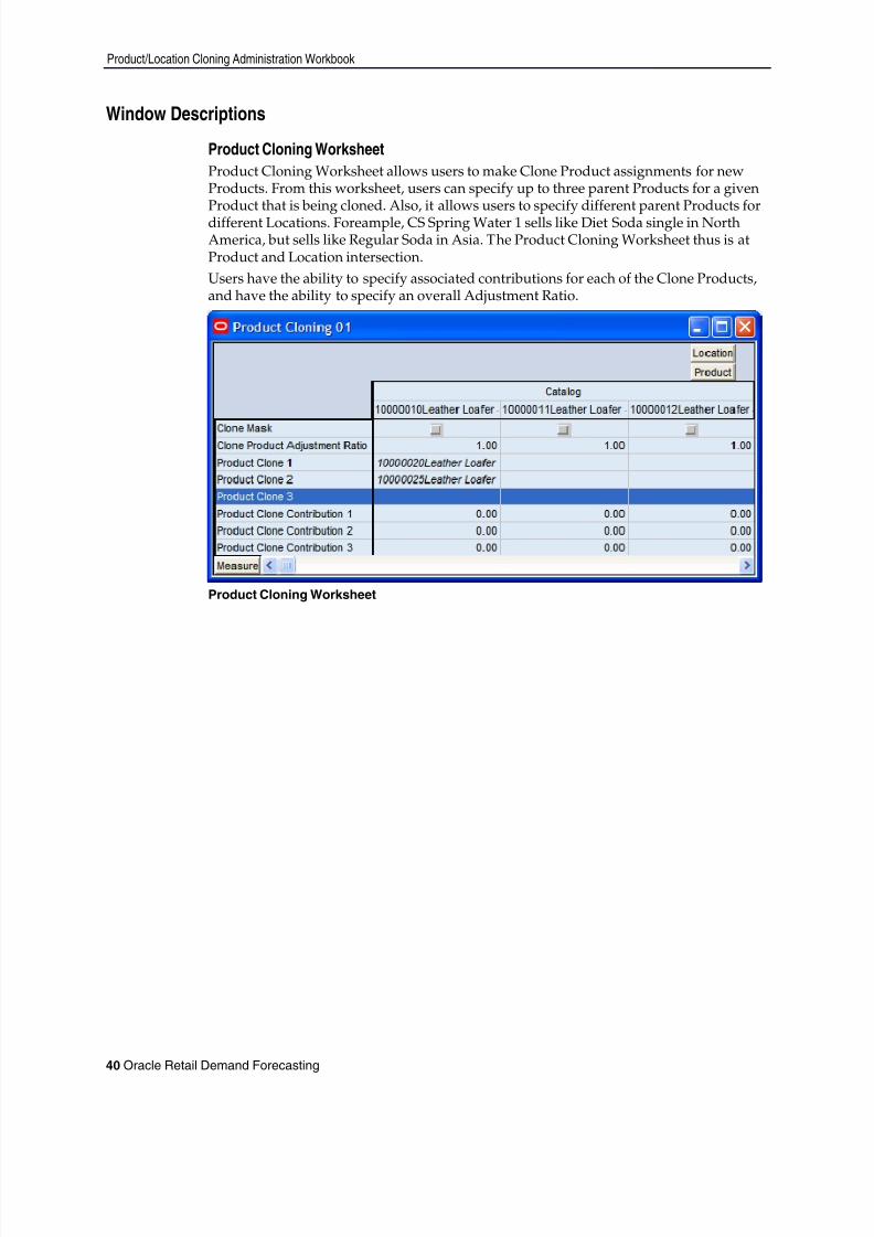
8/10/2019 RDF User Guide
http://slidepdf.com/reader/full/rdf-user-guide 50/120
Product/Location Cloning Administration Workbook
40 Oracle Retail Demand Forecasting
Window Descriptions
Product Cloning WorksheetProduct Cloning Worksheet allows users to make Clone Product assignments for newProducts. From this worksheet, users can specify up to three parent Products for a givenProduct that is being cloned. Also, it allows users to specify different parent Products fordifferent Locations. Foreample, CS Spring Water 1 sells like Diet Soda single in NorthAmerica, but sells like Regular Soda in Asia. The Product Cloning Worksheet thus is atProduct and Location intersection.Users have the ability to specify associated contributions for each of the Clone Products,and have the ability to specify an overall Adjustment Ratio.
Product Cloning Worksheet

8/10/2019 RDF User Guide
http://slidepdf.com/reader/full/rdf-user-guide 51/120
Product/Location Cloning Administration Workbook
Setting Forecast Parameters 41
Field DescriptionsThe Product Cloning Worksheet contains the following measures:
Product Clone1, Product Clone 3, Product Clone 3Parent Products for the new Product being cloned. It is optional to specify more than oneProduct Clone. The selection or assignment of Product Clone is made by clicking on thismeasure and a Single Hier Select Wizard pops up. Assignments are made by selecting aProduct and clicking OK. Please see the RPAS User Guide for more details on the SingleHier Select Wizard.
Product Clone Contribution1, Product Clone Contribution2, Product Clone Contribution3Relative contributions of all clone Products. If user does not specify contributions, butmakes selections for Product Clones and commits the changes, at the time of commit thecontributions are calculated to have equal weights for all specified Product Clones. Ifuser specifies Product clone contributions, they get normalized such that they add up toone at the time of commit. Product Clone contributions with no associated Product Clonevalues get set to zero at the time of commit.
Clone Product Adjustment RatioThe user may enter an Adjustment Ratio to apply to the cloned history of the newproduct. This is a real number between [0, ∞) . The default (NA) value is 1.00, (in otherwords 100%) which translates to no adjustment.
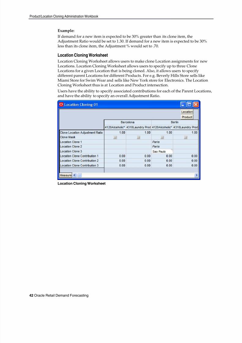
8/10/2019 RDF User Guide
http://slidepdf.com/reader/full/rdf-user-guide 52/120
Product/Location Cloning Administration Workbook
42 Oracle Retail Demand Forecasting
Example:If demand for a new item is expected to be 30% greater than its clone item, theAdjustment Ratio would be set to 1.30. If demand for a new item is expected to be 30%less than its clone item, the Adjustment % would set to .70.
Location Cloning WorksheetLocation Cloning Worksheet allows users to make clone Location assignments for newLocations. Location Cloning Worksheet allows users to specify up to three CloneLocations for a given Location that is being cloned. Also, it allows users to specifydifferent parent Locations for different Products. For e.g. Beverly Hills Store sells likeMiami Store for Swim Wear and sells like New York store for Electronics. The LocationCloning Worksheet thus is at Location and Product intersection.Users have the ability to specify associated contributions for each of the Parent Locations,and have the ability to specify an overall Adjustment Ratio.
Location Cloning Worksheet
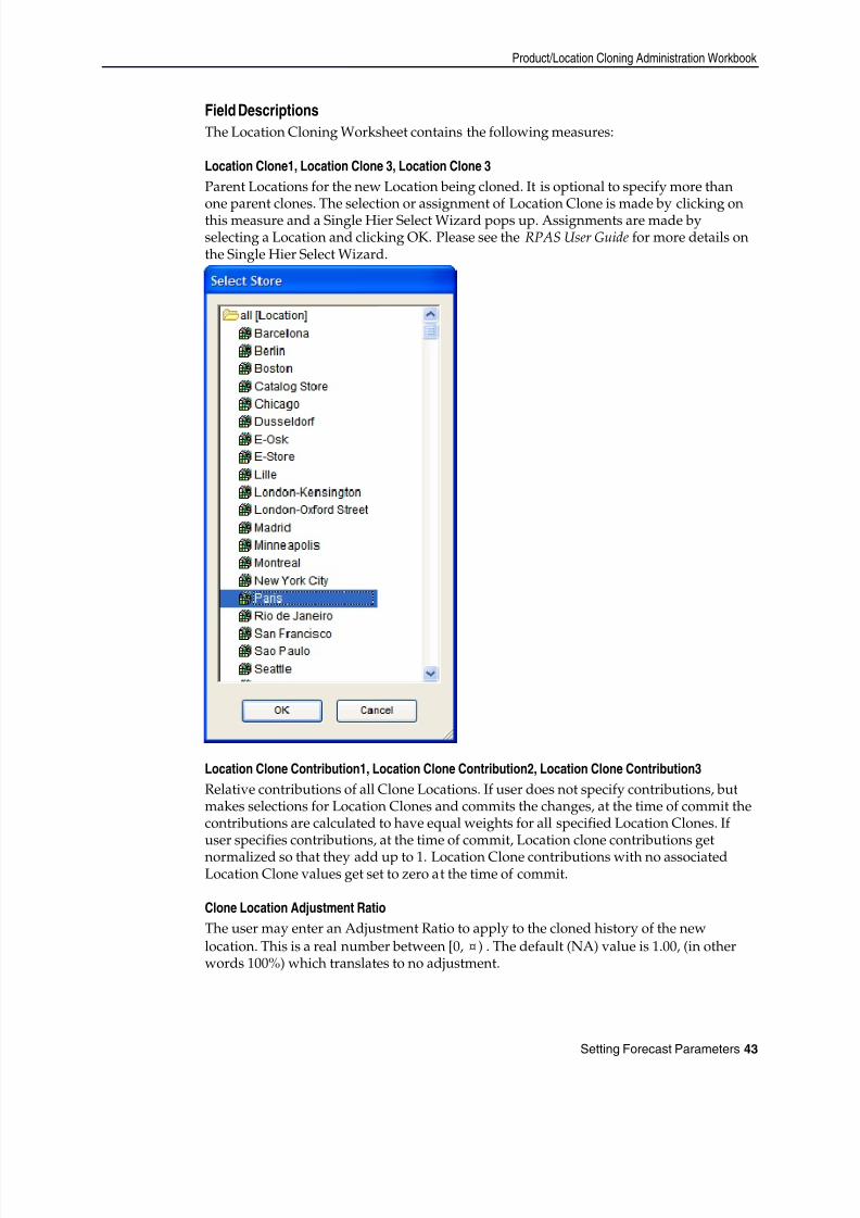
8/10/2019 RDF User Guide
http://slidepdf.com/reader/full/rdf-user-guide 53/120
Product/Location Cloning Administration Workbook
Setting Forecast Parameters 43
Field DescriptionsThe Location Cloning Worksheet contains the following measures:
Location Clone1, Location Clone 3, Location Clone 3Parent Locations for the new Location being cloned. It is optional to specify more thanone parent clones. The selection or assignment of Location Clone is made by clicking onthis measure and a Single Hier Select Wizard pops up. Assignments are made byselecting a Location and clicking OK. Please see the RPAS User Guide for more details onthe Single Hier Select Wizard.
Location Clone Contribution1, Location Clone Contribution2, Location Clone Contribution3Relative contributions of all Clone Locations. If user does not specify contributions, butmakes selections for Location Clones and commits the changes, at the time of commit thecontributions are calculated to have equal weights for all specified Location Clones. Ifuser specifies contributions, at the time of commit, Location clone contributions getnormalized so that they add up to 1. Location Clone contributions with no associatedLocation Clone values get set to zero at the time of commit.
Clone Location Adjustment RatioThe user may enter an Adjustment Ratio to apply to the cloned history of the newlocation. This is a real number between [0, ∞) . The default (NA) value is 1.00, (in otherwords 100%) which translates to no adjustment.
8/10/2019 RDF User Guide
http://slidepdf.com/reader/full/rdf-user-guide 54/120
Product/Location Cloning Administration Workbook
44 Oracle Retail Demand Forecasting
Example:If demand for a new store is expected to be 30% greater than its clone store, theAdjustment Ratio would be set to 1.30. If demand for a new store is expected to be 30%less than its clone store, the Adjustment % would set to .70.
Note: Adjustment Ratios and Clone Contributions specified
in the Product Cloning and Location Cloning Worksheetsare used together while evaluating the result for a givenItem/Store.
Example:SKU1
SKU2 SKU3
20% 80%
Adjustment Ratio = 1STR1:
STR2 STR3
50% 50%
Adjustment Ratio = 0.5The contributions are calculated as:SKU2/STR2 at 5% (=20% x 0.5x50%); SKU2/STR3 at 5%;SKU3/STR2 at20%(=80%x0.5x50%);SKU3/STR3 at 20%
Clone Mask WorksheetThis Worksheet allows users to enable cloning for Product/Locations by setting theClone Mask measure to true.
Note: Clone Mask measure can also be brought in using theShow/Hide option in the Product Cloning and LocationWorksheets. The clone mask can also be set based on
business rules by configuring RPAS rules.

8/10/2019 RDF User Guide
http://slidepdf.com/reader/full/rdf-user-guide 55/120
Generating and Approving a Forecast 45
3Generating and Approving a Forecast
OverviewOnce a user has completed setting all global and individual forecast parameters aforecast must be generated and approved. The Forecast Workbook template groupprovides the workbooks necessary to support these tasks.
Run a Batch Forecast
OverviewThe forecast generation process creates demand forecasts for all product/locationcombinations that are set to forecast within the forecast horizon window. Forecasts aretypically run automatically as scheduled batch jobs. Oracle Retail Demand Forecastingregularly triggers a set of processes to be run at a pre-determined time when system useis at a minimum, such as overnight.Scheduling of the automatic batch forecasting process is supported in part through theForecast Administration Workbook where a default value is set for the forecast cycle(number of days between forecast runs). The Forecast Cycle measure and Next Run Datefield in the Forecast Administration Workbook support the automatic scheduling of
batch forecasting jobs in the Oracle Retail Demand Forecasting solution. Refer to theForecast Administration Workbook description for further information.The Run Batch Forecast wizard allows the user to manually execute the forecastgeneration process at a time other than the regularly scheduled batch job. If a GlobalDomain environment is implemented, forecasts generated in the Local domain can beviewed in the Master domain, however this forecast is isolated to the data in the Localdomain. The execution of “PreGenerateForecast” at the Master domain, then passing theoutput of the process to “Generate” from the backend of each Local domain allows forthe Local domains to share a birth date, thus supporting a view to forecast data acrossLocal domains in the Master domain. See the RDF Administration Guide for moreinformation on “PreGenerateForecast” and “Generate.”Prior to using the Run Batch Forecast wizard, at minimum the following tasks must beperformed:1. Create or access a Forecast Administration Workbook.2. In the Forecast Start Date measure, enter the starting date of the forecast horizon;
otherwise the system will default to the system date (today).3. Set a Default Forecasting Method for the Final and Source Level.
4.
Set a Default Source Level for the Final Level.5. Set the Forecast Length if there is no value already in this measure.6. Set the Spreading Profile if the Source Level(s) are at aggregate dimensions above the
Final Level.7. Commit any changes by selecting File – Commit Now .8. Close the workbook.
8/10/2019 RDF User Guide
http://slidepdf.com/reader/full/rdf-user-guide 56/120
Delete Forecasts
46 Oracle Retail Demand Forecasting
Procedures
Run a Batch Forecast Manually1. Within the Local or Simple domain, select New from the File menu.2. Select the Forecast tab to display a list of workbook templates for statistical
forecasting. Highlight Run Batch Forecast and click OK .3. The Run Batch Forecast Wizard opens and prompts the user to select the FinalLevel(s) to forecast. Select Next or Finish .
The Run Batch wizard automatically executes “PreGenerateForecast” and “Generate”within the Simple or Local Domain. If Next is selected from the last wizard screen, thewizard will not advance to the completion message until the forecast has been generated.Depending on the amount of product/locations to be forecasted and the forecast horizon,it may take a several minutes before the system advances to the final screen. When theforecast generation is completed, the wizard will display a screen that notifies the user ofthe forecast generation ID.After a forecast is generated, the Forecast Start Date field is cleared. This ensures that thesame forecast will not be generated again on the same date. The Next Run Date field is
also updated based on the birth date of the forecast plus the Forecast Cycle. Both fieldscan be viewed in the Forecast Administration workbook.
Delete Forecasts
OverviewThe Days to Keep Forecasts parameter (set in the Forecast Administration workbook)supports the automatic deletion of old forecasts when the Run Batch wizard or“PreGenerateForecast” is executed. Occasionally, a user may need to manually delete aforecast. Some reasons might include: A forecast was run with the wrong source levels selected.
The forecast horizon was not properly set. Old forecasts need to be deleted to save space on the server.
The Delete Forecasts Wizard guides you through the process of deleting unwantedforecasts from the system. Deletions of forecasts are permanent.
Permanently Removing a Forecast from the Oracle Retail Demand Forecasting SystemIf the Delete Forecast wizard is used in a Global Domain environment, deleting a forecastin the Master domain deletes the selected birth date within all domains. Deleting aforecast in the Local domain deletes the selected birth date only within the Local domain.1. From the Simple domain, Master domain, or Local domain; select New from the File
menu.
2.
Select the Forecast tab to display a list of workbook templates for demandforecasting.3. Select Delete Forecasts 4. Click OK .5. Select the forecast generation date(s) of the forecast to delete.6. Click Next .7. Select Yes to verify forecast deletion, or No to cancel deletion and exit the Forecast
Deletion Wizard.
8/10/2019 RDF User Guide
http://slidepdf.com/reader/full/rdf-user-guide 57/120
Forecast Approval Workbook
Generating and Approving a Forecast 47
Note: The deletion of forecasts from Oracle Retail DemandForecasting is permanent.
8. Click Finish to process the request. If Yes was selected on the final wizard screen, theforecast is deleted.
Forecast Approval WorkbookOverview
After the forecast is generated, the next steps in the forecasting process are analysis andapproval. Approval of forecasts is required before the forecasted data can be exported toother processes, such as replenishment programs. The Forecast Approval Workbookallows you to view, analyze, adjust, and approve forecast results.Some system forecasts may be set to be automatically approved by the system. Thedefault approval method for items in a forecast is set in the Forecast AdministrationWorkbook, and these policies can be amended for individual product/locationcombinations in the Forecast Maintenance Workbook. Any forecasts not set to Automatic
Approval may require evaluation, adjustments, and ultimately approval beforesubsequent processes are executed.You can view and analyze forecast data at multiple forecast levels (source level and finallevel) simultaneously. Revisions to and approvals of final level forecast values are madeon the appropriate worksheets in the Forecast Approval Workbook. The ForecastApproval Workbook can contain up to five types of worksheets: Final Forecast Worksheet – This worksheet allows you to review final level system-
forecasted quantities and make revisions to them if needed Source Level Worksheet – This worksheet displays the system-generated source
level forecast, and allows you to compare this data with final level forecast values. Approval Worksheet – This worksheet allows you to specify the manual approval
policy of forecasts by product and location. Final System Parameters Worksheet – This option is only available if “Generate
System Parameters” or “Generate Methods” is turned on in the ForecastAdministration Workbook.
Source System Parameters Worksheet(s) – This option is only available if “GenerateSystem Parameters” or “Generate Methods” is turned on in the ForecastAdministration Workbook, and a Source Level was designated in ForecastAdministration.
Valid Forecast Run Worksheet – This worksheet allows you to review the partitiondimensions in which the generated forecast was run.
When the Forecast Approval Workbook is displayed, you may review the system-generated forecast and measures for any levels included in the workbook and makeadjustments to forecast values at the final level. Forecast values are overwritten in theAdjusted Forecast measure on the Final Forecast Worksheet. Approvals are made foreach product/location combination in the Approval Method measure of the ForecastApproval Worksheet.

8/10/2019 RDF User Guide
http://slidepdf.com/reader/full/rdf-user-guide 58/120
Forecast Approval Workbook
48 Oracle Retail Demand Forecasting
After you complete your work, you can save the workbook using the Save function onthe File menu. To update the master database with the approved forecast values, youmust commit the workbook using the Commit Now or Commit Later option on the Filemenu. Once the workbook is committed, the forecast values are stored in the masterdatabase and can be used by other processes.
Opening or Creating the Forecast Approval WorkbookSelect Open from the File menu to bypass the Forecast Approval Wizard and open anexisting Forecast Approval WorkbookOR1. Within the Master domain, Simple domain, or Local Domain; select New from the
File menu.2. Select the Forecast tab to display a list of workbook templates for statistical
forecasting.3. Select Forecast Approval . Click OK .4. The Forecast Approval wizard opens and prompts you to select the final level at
which to approve forecast values. Make your selection Click Next .5. Select the forecast level(s) to include in the Forecast Approval Workbook. Select as
many forecast levels as necessary for comparison. Click Next .6. Select the birth date of the forecast you wish to approve.
Select Use the most recently generated forecast to build a workbook containingthe most recent forecast values.
Note: Use the most recently generated forecast must beselected if the workbook supports an AutoWorkbook build.
Click Select from a list of forecast to select from a list of previously generatedforecasts stored in the system. Note that if this option is selected, the system willautomatically highlight the first forecast in the list, and if no further selections
are made by the user, this first forecast will be used. If no selection is made by the user, the birth date defaults to the latest generatedgeneration ID.
Click Next .7. Select the specific locations you want to view. It is important to include all locations
that are members of the location dimensions in the forecast levels to be analyzed. Forexample, if you select to view a forecast level that is defined at item/chain/week,you should include all locations that are members of the particular chain to beanalyzed. It is recommended that “Position Query” functionality or selection fromaggregate levels in the Location hierarchy is employed if the workbook is generatedusing AutoWorkbook build. Click Next .
8. Select the merchandise you want to view. It is important to include all products thatare members of the Merchandise dimensions in the forecast levels to be analyzed. Forexample, if you select to view a forecast level that is defined at subclass/store/week,you must include all items that are members of the particular subclass to beanalyzed. It is recommended that “Position Query” functionality or selection fromaggregate levels in the Merchandise hierarchy is employed if the workbook isgenerated using AutoWorkbook build. Click Next .
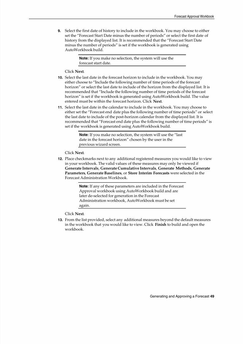
8/10/2019 RDF User Guide
http://slidepdf.com/reader/full/rdf-user-guide 59/120
Forecast Approval Workbook
Generating and Approving a Forecast 49
9. Select the first date of history to include in the workbook. You may choose to eitherset the “Forecast Start Date minus the number of periods” or select the first date ofhistory from the displayed list. It is recommended that the “Forecast Start Dateminus the number of periods” is set if the workbook is generated usingAutoWorkbook build.
Note: If you make no selection, the system will use theforecast start date.
Click Next .10. Select the last date in the forecast horizon to include in the workbook. You may
either choose to “Include the following number of time periods of the forecasthorizon” or select the last date to include of the horizon from the displayed list. It isrecommended that “Include the following number of time periods of the forecasthorizon” is set if the workbook is generated using AutoWorkbook build. The valueentered must be within the forecast horizon. Click Next .
11. Select the last date in the calendar to include in the workbook. You may choose toeither set the “Forecast end date plus the following number of time periods” or selectthe last date to include of the post-horizon calendar from the displayed list. It isrecommended that “Forecast end date plus the following number of time periods” isset if the workbook is generated using AutoWorkbook build.
Note: If you make no selection, the system will use the “lastdate in the forecast horizon” chosen by the user in theprevious wizard screen.
Click Next .12. Place checkmarks next to any additional registered measures you would like to view
in your workbook. The valid values of these measures may only be viewed ifGenerate Intervals , Generate Cumulative Intervals , Generate Methods , GenerateParameters , Generate Baselines , or Store Interim Forecasts were selected in theForecast Administration Workbook.
Note: If any of these parameters are included in the ForecastApproval workbook using AutoWorkbook build and arelater de-selected for generation in the ForecastAdministration workbook, AutoWorkbook must be setagain.
Click Next .13. From the list provided, select any additional measures beyond the default measures
in the workbook that you would like to view. Click Finish to build and open theworkbook.

8/10/2019 RDF User Guide
http://slidepdf.com/reader/full/rdf-user-guide 60/120
Forecast Approval Workbook
50 Oracle Retail Demand Forecasting
Window Descriptions
Final Forecast WorksheetThe Final Forecast Worksheet allows you to review the forecasted quantities and makeadjustments to forecasts if needed. The primary objective in the Forecast ApprovalWorkbook is to review and edit forecast values using the Adjusted Forecast field on theFinal Level Worksheet and, ultimately approve forecasts that have been user-adjusted orrequire manual approval.
Final Level Worksheet
Field DescriptionsThe following is a description of the standard measures that are contained in the FinalLevel Worksheet:
Adjusted Cumulative IntervalWhen changes are made to the Adjusted Forecast, the value of the Forecast CumulativeInterval is recalculated in this measure. The values in this measure are read-only. Toview and store this measure: Generate Cumulative Intervals must be selected in the Forecast Administration
Workbook Cumulative Intervals must be selected to be viewed in the Forecast Approval wizard.
Adjusted Forecast
The value in this field initially defaults to the System Forecast if the forecast isautomatically approved by the system or via a Forecast Approval Alert. Otherwise, thevalue in the Adjusted Forecast will be different than the System Forecast if:1. Adjusted Forecast has been updated by the user2. Keep Last Changes is set to Total , Difference or Ratio 3. Update Last Week(s) Forecast is set to Replicate

8/10/2019 RDF User Guide
http://slidepdf.com/reader/full/rdf-user-guide 61/120
Forecast Approval Workbook
Generating and Approving a Forecast 51
Changes to the Adjusted Forecast will be automatically approved. The ApprovalWorksheet will update with the date of the adjustment the name of the user to make theadjustment.
Note: Changes to the Adjusted Forecast for periods outsideof the forecast horizon will not be committed.
Note: Edits to any non-committed values in the ForecastApproval workbook are overwritten when data is‘Refreshed.’
Approved Cumulative IntervalThe Approved Cumulative Interval is the cumulative interval that was approved at thetime of the workbook build. The values contained in this measure are read-only. Ifchanges are made to the Adjusted Forecast, the Approved Cumulative Interval willreflect the recalculated values when the workbook is committed and data is refreshed.
Approved ForecastThe Approved Forecast is the forecast quantity that was approved at the time of theworkbook build. The values contained in this measure are read-only. If changes are madeto the Adjusted Forecast, the Approved Forecast will update with the new values whenthe workbook is committed and data is refreshed.
Approved System ForecastThe Approved System Forecast is populated with the last System Forecast approved for atime series:1. Approval Method set to Automatic Approval 2. Approval Method set to a Forecast Approval Alert and the alert is not triggered3. Update Last Week(s) Forecast is set to Use Forecast The values in this measure are read-only.
Forecast Cumulative IntervalCumulative Intervals are used in safety stock calculation within allocation andreplenishment systems. This value is similar to a running total of the Forecast Intervaland is read-only. To see this measure: Generate Cumulative Intervals must be selected in the Forecast Administration
Workbook. Cumulative Intervals must be selected to be viewed in the Forecast Approval
wizard.
Forecast IntervalThe Forecast Interval is calculated on the particular forecast region as capped standarddeviation for some methods. It takes into consideration the system forecast for capping(the default capping is no less than 30% of forecast and no more than 100% of forecast).When we approve forecasts, we approve the corresponding Intervals and CumulativeInterval measures. To see this measure: Generate Intervals must be selected in the Forecast Administration Workbook. Intervals must be selected to be viewed in the Forecast Approval wizard.
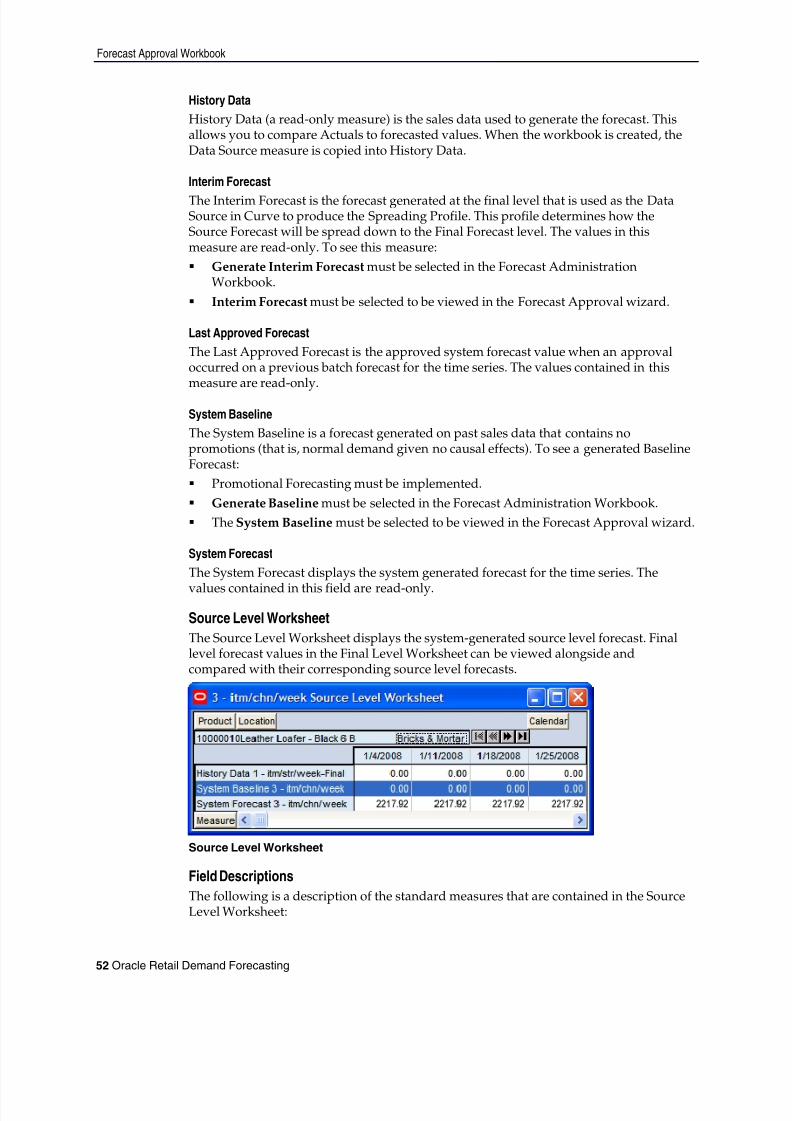
8/10/2019 RDF User Guide
http://slidepdf.com/reader/full/rdf-user-guide 62/120
Forecast Approval Workbook
52 Oracle Retail Demand Forecasting
History DataHistory Data (a read-only measure) is the sales data used to generate the forecast. Thisallows you to compare Actuals to forecasted values. When the workbook is created, theData Source measure is copied into History Data.
Interim Forecast
The Interim Forecast is the forecast generated at the final level that is used as the DataSource in Curve to produce the Spreading Profile. This profile determines how theSource Forecast will be spread down to the Final Forecast level. The values in thismeasure are read-only. To see this measure: Generate Interim Forecast must be selected in the Forecast Administration
Workbook. Interim Forecast must be selected to be viewed in the Forecast Approval wizard.
Last Approved ForecastThe Last Approved Forecast is the approved system forecast value when an approvaloccurred on a previous batch forecast for the time series. The values contained in thismeasure are read-only.
System BaselineThe System Baseline is a forecast generated on past sales data that contains nopromotions (that is, normal demand given no causal effects). To see a generated BaselineForecast: Promotional Forecasting must be implemented. Generate Baseline must be selected in the Forecast Administration Workbook. The System Baseline must be selected to be viewed in the Forecast Approval wizard.
System ForecastThe System Forecast displays the system generated forecast for the time series. The
values contained in this field are read-only.
Source Level WorksheetThe Source Level Worksheet displays the system-generated source level forecast. Finallevel forecast values in the Final Level Worksheet can be viewed alongside andcompared with their corresponding source level forecasts.
Source Level Worksheet
Field DescriptionsThe following is a description of the standard measures that are contained in the SourceLevel Worksheet:
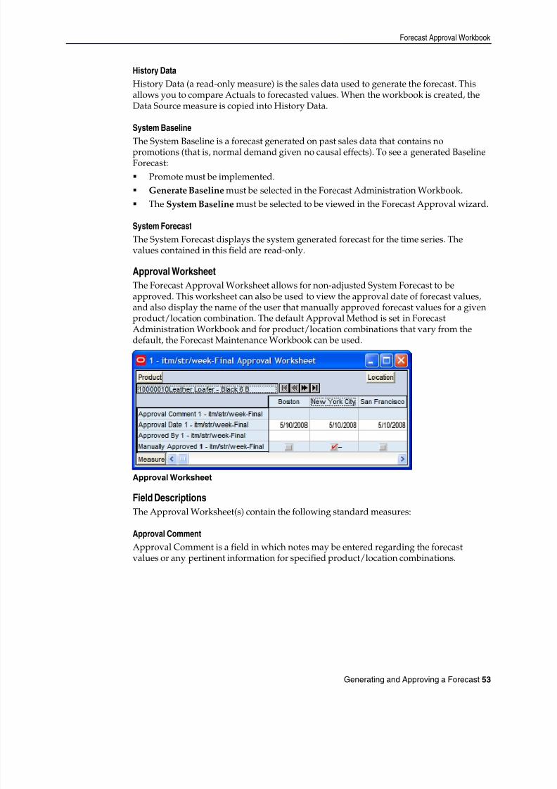
8/10/2019 RDF User Guide
http://slidepdf.com/reader/full/rdf-user-guide 63/120
Forecast Approval Workbook
Generating and Approving a Forecast 53
History DataHistory Data (a read-only measure) is the sales data used to generate the forecast. Thisallows you to compare Actuals to forecasted values. When the workbook is created, theData Source measure is copied into History Data.
System Baseline
The System Baseline is a forecast generated on past sales data that contains nopromotions (that is, normal demand given no causal effects). To see a generated BaselineForecast: Promote must be implemented. Generate Baseline must be selected in the Forecast Administration Workbook. The System Baseline must be selected to be viewed in the Forecast Approval wizard.
System ForecastThe System Forecast displays the system generated forecast for the time series. Thevalues contained in this field are read-only.
Approval WorksheetThe Forecast Approval Worksheet allows for non-adjusted System Forecast to beapproved. This worksheet can also be used to view the approval date of forecast values,and also display the name of the user that manually approved forecast values for a givenproduct/location combination. The default Approval Method is set in ForecastAdministration Workbook and for product/location combinations that vary from thedefault, the Forecast Maintenance Workbook can be used.
Approval Worksheet
Field DescriptionsThe Approval Worksheet(s) contain the following standard measures:
Approval CommentApproval Comment is a field in which notes may be entered regarding the forecastvalues or any pertinent information for specified product/location combinations.
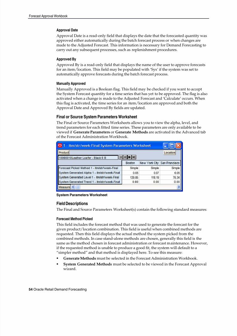
8/10/2019 RDF User Guide
http://slidepdf.com/reader/full/rdf-user-guide 64/120
Forecast Approval Workbook
54 Oracle Retail Demand Forecasting
Approval DateApproval Date is a read-only field that displays the date that the forecasted quantity wasapproved either automatically during the batch forecast process or when changes aremade to the Adjusted Forecast. This information is necessary for Demand Forecasting tocarry out any subsequent processes, such as replenishment procedures.
Approved ByApproved By is a read-only field that displays the name of the user to approve forecastsfor an item/location. This field may be populated with ‘Sys’ if the system was set toautomatically approve forecasts during the batch forecast process.
Manually ApprovedManually Approved is a Boolean flag. This field may be checked if you want to acceptthe System Forecast quantity for a time series that has yet to be approved. The flag is alsoactivated when a change is made to the Adjusted Forecast and ‘Calculate’ occurs. Whenthis flag is activated, the time series for an item/location are approved and both theApproval Date and Approved By fields are updated.
Final or Source System Parameters WorksheetThe Final or Source Parameters Worksheets allows you to view the alpha, level, andtrend parameters for each fitted time series. These parameters are only available to beviewed if Generate Parameters or Generate Methods are activated in the Advanced tabof the Forecast Administration Workbook.
System Parameters Worksheet
Field DescriptionsThe Final and Source Parameters Worksheet(s) contain the following standard measures:
Forecast Method PickedThis field includes the forecast method that was used to generate the forecast for thegiven product/location combination. This field is useful when combined methods are
requested. Then this field displays the actual method the system picked from thecombined methods. In case stand-alone methods are chosen, generally this field is thesame as the method chosen in forecast administration or forecast maintenance. However,if the requested method is unable to produce a good fit, the system will default to a“simpler method” and that method is displayed here. To see this measure: Generate Methods must be selected in the Forecast Administration Workbook. System Generated Methods must be selected to be viewed in the Forecast Approval
wizard.
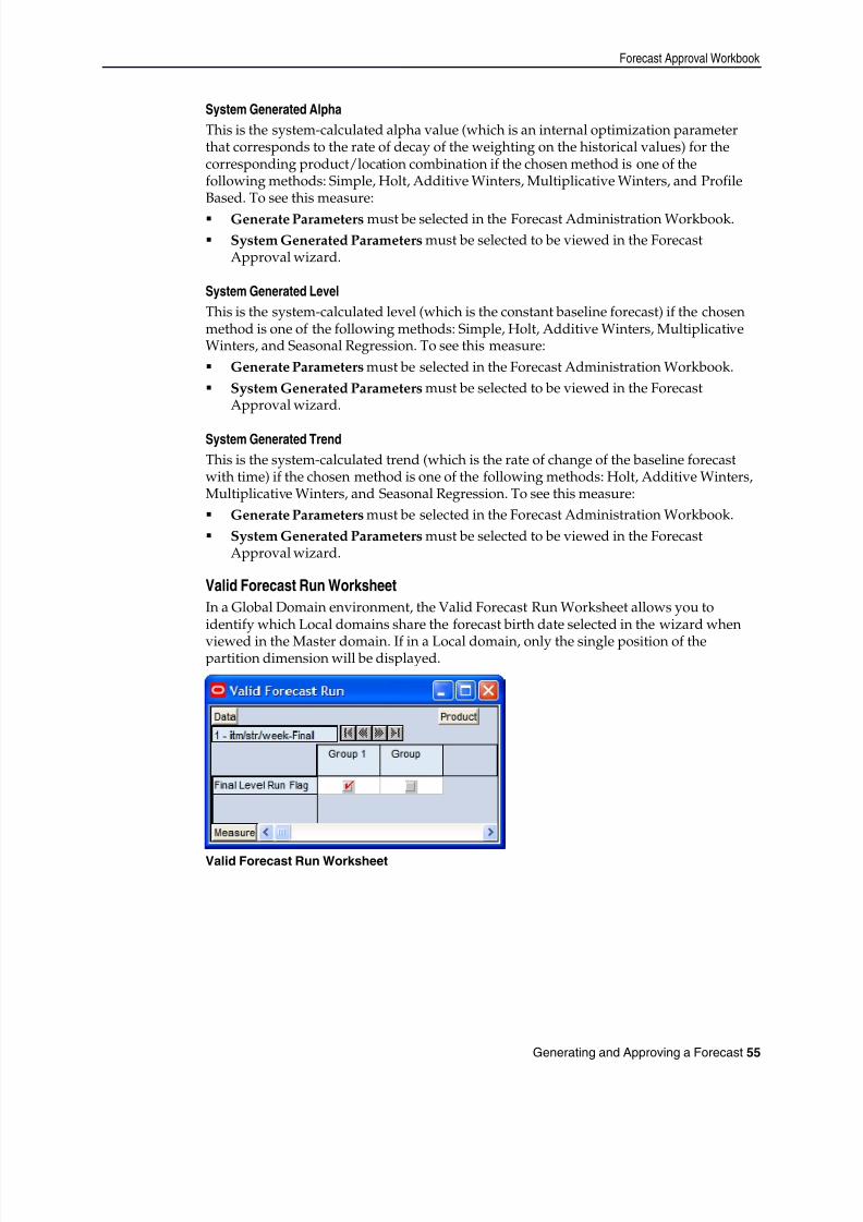
8/10/2019 RDF User Guide
http://slidepdf.com/reader/full/rdf-user-guide 65/120
Forecast Approval Workbook
Generating and Approving a Forecast 55
System Generated AlphaThis is the system-calculated alpha value (which is an internal optimization parameterthat corresponds to the rate of decay of the weighting on the historical values) for thecorresponding product/location combination if the chosen method is one of thefollowing methods: Simple, Holt, Additive Winters, Multiplicative Winters, and ProfileBased. To see this measure: Generate Parameters must be selected in the Forecast Administration Workbook. System Generated Parameters must be selected to be viewed in the Forecast
Approval wizard.
System Generated LevelThis is the system-calculated level (which is the constant baseline forecast) if the chosenmethod is one of the following methods: Simple, Holt, Additive Winters, MultiplicativeWinters, and Seasonal Regression. To see this measure: Generate Parameters must be selected in the Forecast Administration Workbook. System Generated Parameters must be selected to be viewed in the Forecast
Approval wizard.
System Generated TrendThis is the system-calculated trend (which is the rate of change of the baseline forecastwith time) if the chosen method is one of the following methods: Holt, Additive Winters,Multiplicative Winters, and Seasonal Regression. To see this measure: Generate Parameters must be selected in the Forecast Administration Workbook. System Generated Parameters must be selected to be viewed in the Forecast
Approval wizard.
Valid Forecast Run WorksheetIn a Global Domain environment, the Valid Forecast Run Worksheet allows you toidentify which Local domains share the forecast birth date selected in the wizard when
viewed in the Master domain. If in a Local domain, only the single position of thepartition dimension will be displayed.
Valid Forecast Run Worksheet
8/10/2019 RDF User Guide
http://slidepdf.com/reader/full/rdf-user-guide 66/120
Approving Forecasts through Alerts (Exception Management)
56 Oracle Retail Demand Forecasting
Field DescriptionsThe measure displayed on this worksheet is viewed at final level / partition intersection.The Valid Forecast Run Worksheet includes the following standard measure:
Final Level Run FlagThe Final Level Run Flag is a read-only Boolean measure. A check (set to true) displayedin this field indicates which positions from the partition dimension had a successfulforecast run for the birth date selected in the Forecast Approval wizard.
Note: Edits to the Adjusted Forecast can only be committedfor partitions that have an activated Final Level Run Flag.
Approving Forecasts through Alerts (Exception Management)
OverviewOracle Retail Demand Forecasting provides you with ability to manually approve everysingle product/location forecast value. However, due to the extremely large volume of
product/location forecast values that will be generated for each forecast cycle, RPASprovides additional functionality that enhances your ability to evaluate and approve aforecast.When configuring an RDF solution, specific Forecast Approval Alerts and alertparameters may be defined and applied during the batch process, and they may also beinserted into the Forecast Approval Workbook. Alerts report product/location forecastvalues that exceed expected thresholds. If a specific product/location forecast valueexceeds a threshold, the alert measure is flagged as “on” and visible to the user as a checkmark in the appropriate product/location intersection. The complexities of retail operations can result in the need to define many alerts;
each designed to watch for a specific scenario that would require a user’s evaluationof a forecast value.
For more information on how alert measures and rules are defined and registered, referto the R PAS Configuration Tools User Guide and RDF Administration Guide .

8/10/2019 RDF User Guide
http://slidepdf.com/reader/full/rdf-user-guide 67/120
Forecast Analysis Tools 57
4Forecast Analysis Tools
OverviewOracle Retail Demand Forecasting provides you with a number of tools that may be usedfor additional forecast analysis. The Forecast Workbook template group provides theworkbooks necessary to complete these tasks.
Interactive Forecasting Workbook
OverviewThe Interactive Forecasting Workbook is a forecast simulation tool that allows you tomake changes to forecast parameters and see the results without having to wait for the
batch run. In this workbook, you can edit various forecast parameters including saleshistory and forecast method. A new forecast is produced based on the changedparameters. In addition to forecasts, the Interactive Forecasting Workbook can alsogenerate fit in historical region and the system picked model if an ES forecast method isused.
Opening the Interactive Forecasting Workbook1. Within the Local or Simple domain, select New from the File menu.2. Select the Forecast tab to display a list of workbook templates.3. Select Interactive Forecastin g. Click OK .4. Select the forecast level. Click Next .5. Select the forecast starting date. Click Next .6. Select the first date in the historical data to use for generating the forecast. Click
Next .7. Select the end date for the forecast horizon. Click Next .8. Perform one of the following options:
Specify future time periods beyond the forecast horizon to include in yourworkbook.
Select Do not include dates after the horizon if no future dates are to be includedin the workbook.
Click Next .9. Select the products to be included in the workbook. Click Next .10. Select the locations to be included in the workbook. Click Next .11. Select extra measures (if needed) to be included in the forecasting workbook. Click
Finish .Once the wizard is completed, the forecast is generated based on the user selections inthe wizard and the Default Forecast Method set for the specified forecast level in theForecast Administration Workbook.
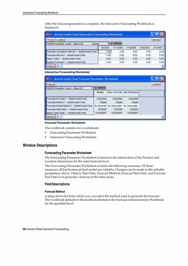
8/10/2019 RDF User Guide
http://slidepdf.com/reader/full/rdf-user-guide 68/120
Interactive Forecasting Workbook
58 Oracle Retail Demand Forecasting
After the forecast generation is complete, the Interactive Forecasting Workbook isdisplayed.
Interactive Forecasting Worksheet
Forecast Parameter Worksheet
The workbook contains two worksheets: Forecasting Parameter Worksheet Interactive Forecasting Worksheet
Window Descriptions
Forecasting Parameter WorksheetThe Forecasting Parameter Worksheet is based on the intersection of the Product andLocation dimensions for the select forecast level.The Forecasting Parameter Worksheet contains the following measures. Of thesemeasures, all but System picked model are editable. Changes can be made to the editableparameters, that is, History Start Date, Forecast Method, Forecast Start Date, and ForecastEnd Date to re-generate a forecast of the time series.
Field Descriptions
Forecast MethodA drop-down list from which you can select the method used to generate the forecast.The workbook defaults to the method selected in the Forecast Administration Workbookfor the specified level.
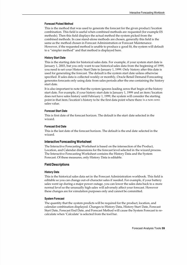
8/10/2019 RDF User Guide
http://slidepdf.com/reader/full/rdf-user-guide 69/120
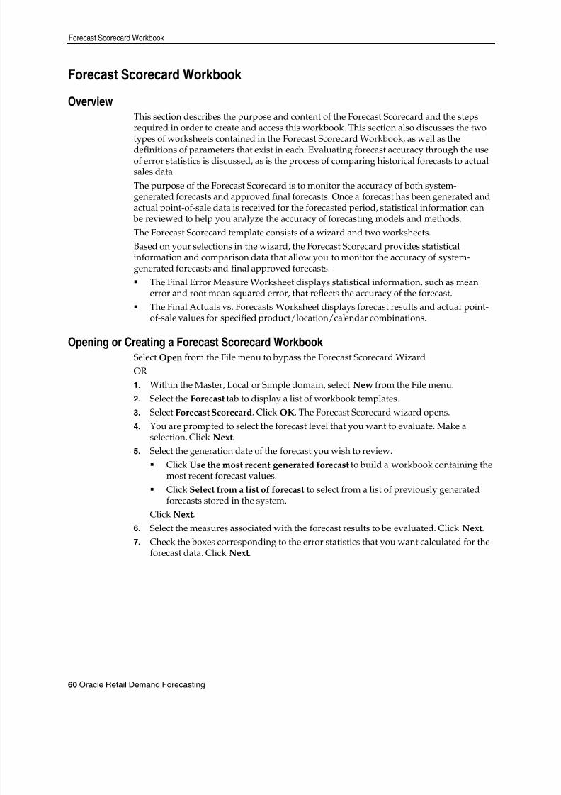
8/10/2019 RDF User Guide
http://slidepdf.com/reader/full/rdf-user-guide 70/120
Forecast Scorecard Workbook
60 Oracle Retail Demand Forecasting
Forecast Scorecard Workbook
OverviewThis section describes the purpose and content of the Forecast Scorecard and the stepsrequired in order to create and access this workbook. This section also discusses the two
types of worksheets contained in the Forecast Scorecard Workbook, as well as thedefinitions of parameters that exist in each. Evaluating forecast accuracy through the useof error statistics is discussed, as is the process of comparing historical forecasts to actualsales data.The purpose of the Forecast Scorecard is to monitor the accuracy of both system-generated forecasts and approved final forecasts. Once a forecast has been generated andactual point-of-sale data is received for the forecasted period, statistical information can
be reviewed to help you analyze the accuracy of forecasting models and methods.The Forecast Scorecard template consists of a wizard and two worksheets.Based on your selections in the wizard, the Forecast Scorecard provides statisticalinformation and comparison data that allow you to monitor the accuracy of system-generated forecasts and final approved forecasts. The Final Error Measure Worksheet displays statistical information, such as mean
error and root mean squared error, that reflects the accuracy of the forecast. The Final Actuals vs. Forecasts Worksheet displays forecast results and actual point-
of-sale values for specified product/location/calendar combinations.
Opening or Creating a Forecast Scorecard WorkbookSelect Open from the File menu to bypass the Forecast Scorecard WizardOR1. Within the Master, Local or Simple domain, select New from the File menu.2. Select the Forecast tab to display a list of workbook templates.3. Select Forecast Scorecard . Click OK . The Forecast Scorecard wizard opens.4. You are prompted to select the forecast level that you want to evaluate. Make a
selection. Click Next .5. Select the generation date of the forecast you wish to review.
Click Use the most recent generated forecast to build a workbook containing themost recent forecast values.
Click Select from a list of forecast to select from a list of previously generatedforecasts stored in the system.
Click Next .6. Select the measures associated with the forecast results to be evaluated. Click Next .7. Check the boxes corresponding to the error statistics that you want calculated for the
forecast data. Click Next .
8/10/2019 RDF User Guide
http://slidepdf.com/reader/full/rdf-user-guide 71/120
Forecast Scorecard Workbook
Forecast Analysis Tools 61
8. Select the specific locations that you want to view. It is important to include alllocations that are members of the location dimensions in the forecast levels to beanalyzed. For example, if you select to view a forecast level that is defined atitem/chain/week, you should include all locations that are members of theparticular chain to be analyzed. It is recommended that “Position Query”functionality or selection from aggregate levels in the Location hierarchy is employed
if the workbook supports an AutoWorkbook build. Make your selection. Click Next .9. Select the merchandise you want to view. It is important to include all products that
are members of the Merchandise dimensions in the forecast levels to be analyzed. Forexample, if you select to view a forecast level that is defined at subclass/store/week,you must include all items that are members of the particular subclass to beanalyzed. It is recommended that “Position Query” functionality or selection fromaggregate levels in the Merchandise hierarchy is employed if the workbook supportsan AutoWorkbook build. Make your selection. Click Next .
10. Select the first date of history to include in the workbook. You may either choose toset the Forecast Start Date minus the number of periods or select the first date ofhistory from the displayed list. It is recommended that the Forecast Start Date minusthe number of periods is set if the workbook supports an AutoWorkbook build.
Make your selection. Click Next .11. Select the last date in the forecast horizon to include in the workbook.
Choose Include the following number of time periods of the forecast horizon .
Note: It is recommended that “Include the following numberof time periods of the forecast horizon” is set if theworkbook supports an AutoWorkbook build.
Select the last date to include of the horizon from the displayed list. Click Next .12. Select the last date in the calendar to include in the workbook.
Set the Forecast end date plus the following number of time periods .
Note: It is recommended that Forecast end date plus thefollowing number of time periods is set if the workbooksupports an AutoWorkbook build.
Select the last date to include of the post-horizon calendar from the displayedlist.
Click Next .13. Select any additional measures to be included in the workbook. Click Finish .
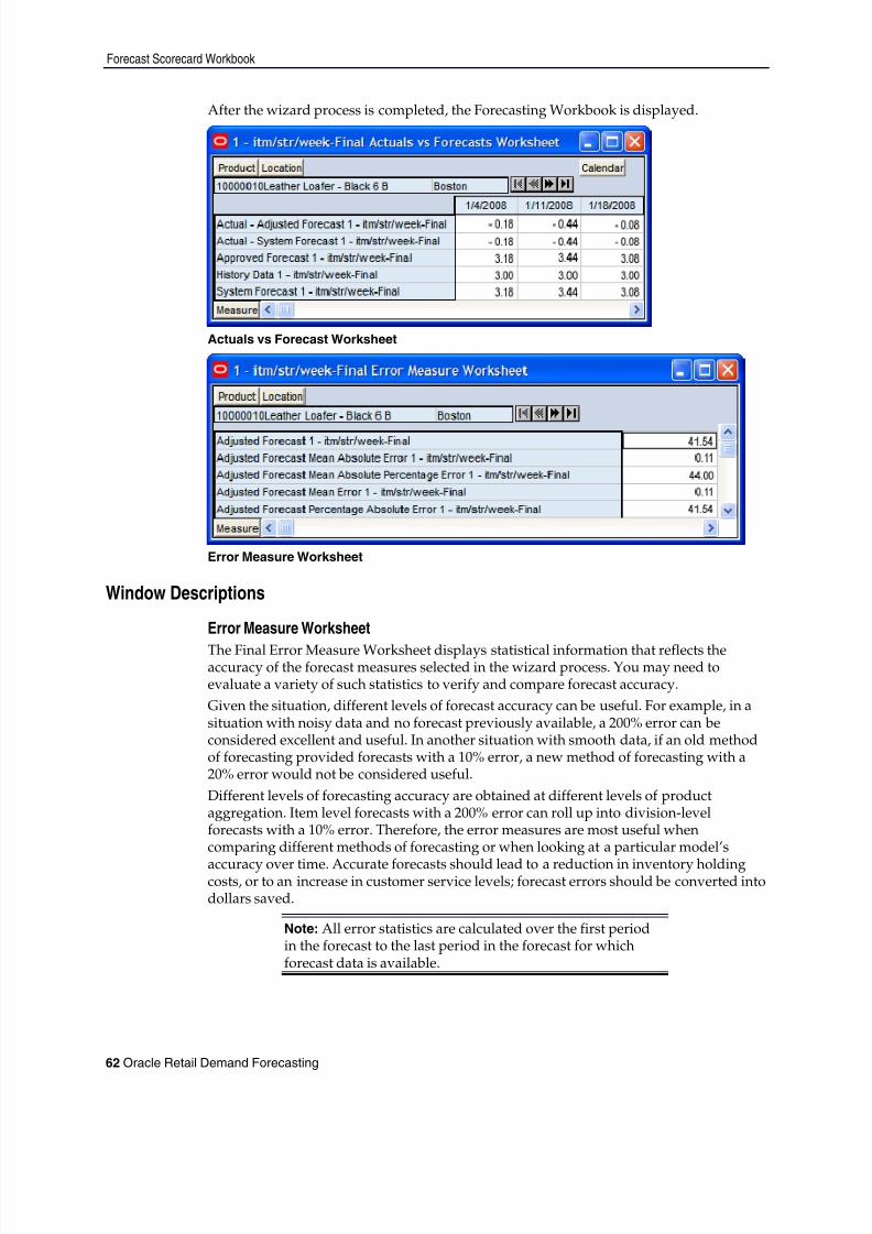
8/10/2019 RDF User Guide
http://slidepdf.com/reader/full/rdf-user-guide 72/120
Forecast Scorecard Workbook
62 Oracle Retail Demand Forecasting
After the wizard process is completed, the Forecasting Workbook is displayed.
Actuals vs Forecast Worksheet
Error Measure Worksheet
Window Descriptions
Error Measure Worksheet
The Final Error Measure Worksheet displays statistical information that reflects theaccuracy of the forecast measures selected in the wizard process. You may need toevaluate a variety of such statistics to verify and compare forecast accuracy.Given the situation, different levels of forecast accuracy can be useful. For example, in asituation with noisy data and no forecast previously available, a 200% error can beconsidered excellent and useful. In another situation with smooth data, if an old methodof forecasting provided forecasts with a 10% error, a new method of forecasting with a20% error would not be considered useful.Different levels of forecasting accuracy are obtained at different levels of productaggregation. Item level forecasts with a 200% error can roll up into division-levelforecasts with a 10% error. Therefore, the error measures are most useful whencomparing different methods of forecasting or when looking at a particular model’s
accuracy over time. Accurate forecasts should lead to a reduction in inventory holdingcosts, or to an increase in customer service levels; forecast errors should be converted intodollars saved.
Note: All error statistics are calculated over the first periodin the forecast to the last period in the forecast for whichforecast data is available.
8/10/2019 RDF User Guide
http://slidepdf.com/reader/full/rdf-user-guide 73/120
Forecast Scorecard Workbook
Forecast Analysis Tools 63
Field DescriptionsThe following is a description of the measures that can be included in the Final ErrorMeasure Worksheet: The error statistics will be shown for each forecast that you chose toinclude in the workbook (such as System Forecast, Final Forecast, and so on).
History Data for Forecast WindowThe sum of all actual sales from the first period in the forecast to the last period in theforecast for which point-of-sale data is available.
System Forecast, Adjusted Forecast, Approved Forecast, Approved System Forecast, InterimForecastYour workbook may include one or all of the above forecast measures. These measuresare selected in the wizard process. This is the average value of these measures over theforecast horizon select in the wizard process.
Mean ErrorThe error of a forecast observation is the difference between the forecasted value and theactual POS value. The Mean Error statistic is a measure of the average error over time.This is calculated by summing the errors for all observations, and then by dividing by thenumber of observations to obtain the average. It measures forecast accuracy bycalculating the error in units. Because a positive error in one period can cancel out anegative error in another period, this measure is useful when you are interested in howwell the forecast predicts over the forecast horizon rather than on a period-to-period
basis. Mean error is useful as a measure of forecast bias. A negative mean error suggeststhat overall the forecasting model overstates the forecast while a positive mean errorindicates forecasts that are generally too low.
Mean Absolute ErrorThe absolute error of a forecast observation is the absolute value of the difference
between the forecasted value and the actual POS value. The Mean Absolute Error statistic
is a measure of the average absolute error. This is calculated by summing the absoluteerrors for all observations, and then by dividing by the number of observations to obtainthe average. Mean Absolute Error gives you a better indication of how the forecastperformed period by period, because the absolute value function ensures that negativeerrors in one period are not canceled out by positive errors in another. Mean AbsoluteError is most useful for comparing two forecast methods for the same series.
Root Mean Squared ErrorThis is the square root of the Mean Squared Error. The Root Mean Squared Error is one ofthe most commonly used measures of forecast accuracy because of its similarity to the
basic statistical concept of a standard deviation. It evaluates the magnitude of errors in aforecast on a period-by-period basis, and it is best used to compare alternativeforecasting models for a given series.
Mean Absolute Percentage ErrorThe percentage error of a forecast observation is the difference between the actual POSvalue and the forecasted value, divided by the actual POS value. The result of thiscalculation expresses the forecast error as a percentage of the actual value. The MeanAbsolute Percentage Error statistic measures forecast accuracy by taking the average ofthe sum of the absolute values of the percentage error calculations across all
8/10/2019 RDF User Guide
http://slidepdf.com/reader/full/rdf-user-guide 74/120
Forecast Scorecard Workbook
64 Oracle Retail Demand Forecasting
observations. This method is useful when comparing the accuracy of forecasts fordifferent volume products (it normalizes error by volume).
Percentage Absolute ErrorThe absolute error of a forecast observation is the absolute value of the difference
between the forecasted value and the actual POS value. The Percentage Absolute Errorstatistic measures forecast accuracy by calculating the total absolute error as a percentageof the total actual POS. It is calculated by summing the absolute errors for allobservations, dividing this value by the absolute value of the sum of all Actuals, anddividing the result by the number of observations in the series. Finally, multiply the total
by 100 to obtain a percentage result.
Actuals vs. Forecasts WorksheetThis worksheet displays forecast results and actual point-of-sale values for each product,location, and time period specified in the Forecast Scorecard Wizard. This worksheetallows you to compare the results of both system-generated forecasts and final approvedforecasts to actual sales quantities.The Actuals vs. Forecasts Worksheet may contain the following measures:
Actuals – (minus) System Forecast, Adjusted Forecast, Approved Forecast, Approved SystemForecast, Interim ForecastThis displays the difference between the actual sales quantities and the committedforecast values for the forecast measures selected during the wizard process. Negativevalues indicate that the final forecast exceeded actual sales.
History DataHistory Data displays the actual point-of-sale quantities for the product, location, andcalendar combinations displayed.
System Forecast, Adjusted Forecast, Approved Forecast, Approved System Forecast, Interim
ForecastYour workbook may include one or all of the above forecast measures. These measuresare selected in the wizard process. These measures display the forecasted quantity for theproduct, location, and calendar combinations included in the workbook.
8/10/2019 RDF User Guide
http://slidepdf.com/reader/full/rdf-user-guide 75/120
Promote (Promotional Forecasting) 65
5Promote (Promotional Forecasting)
OverviewPromote is an optional add-on automated predictive solution that allows you toincorporate the effects of promotional and causal events (such as, radio advertisementsand holiday occurrences) into your time-series forecasts. The promotional forecastingprocess uses both past sales data and promotional information to forecast futuredemand.This chapter provides an introduction to promotional forecasting and explains how itdiffers from the traditional statistical forecasting methodology. It discusses theadvantages and limitations of both statistical and promotional forecasting models, and itoutlines the use of Oracle Retail’s Causal method of forecasting demand. It describesterminology used in the context of promotional forecasting, and it concludes withdetailed descriptions of the workbook templates contained in the Promote WorkbookTemplate Group.
What is Promotional Forecasting?Traditional statistical forecasting methods provide significant benefits to the process offorecasting consumer demand, because they are good at predicting level, trend, andseasonality based on sales history. The limitation of traditional statistical methods is thatthey forecast with less accuracy when there are special events that cause significantdeviations in selling patterns.For example, the Easter holiday, for which companies often run promotions, occurs on adifferent date each year. Traditional statistical forecast methods can identify seasonalityin sales history, but this seasonality is based on periodic similarities in the sales pattern.Since Easter occurs on different dates from year to year (that is, its period of recurrence isnot regular), manual intervention is required to predict change in demand using thetraditional statistical forecasting method. Events like this are called promotion events.Promotion events, such as advertisements, irregularly occurring holidays, competitorinformation, free gift with purchase offers, and so on are events that drive businessesfrom the normal selling cycle. The goal of a promotional forecasting system is to improvetime series forecasting by: Providing the forecasting system with visibility as to when certain promotion events
were active in the past (for example, identifying which weeks of a given year wereaffected by an Easter promotion).
Automatically determining the statistical effect, if any, of these events. Incorporating significant effects into the future forecasts for time periods also
associated with the observed promotion event.The Promote module combines the automation of statistical time series forecasting withthe improved accuracy found in customized causal forecasting. Promote uses both pastsales data and promotional information (for example, advertisements, holidays) toforecast future demand. In order to understand the underlying rationale for thepromotional forecasting process, it is important to understand the advantages andlimitations of its underlying components.

8/10/2019 RDF User Guide
http://slidepdf.com/reader/full/rdf-user-guide 76/120
Overview
66 Oracle Retail Demand Forecasting
Comparison between Promotional and Statistical ForecastingStatistical time series forecasting uses past demand to predict future demand. The most
basic component of the time series forecast is the level of sales. This is usuallydetermined by looking at demand in the recent past. There often exists an underlyingtrend that can be detected within sales history. This is usually determined by looking atthe change in demand in the recent past. A third factor influencing retail demand isseasonality. A forecasting algorithm trying to determine the effects of seasonality canonly look for periodic similarities in the sales pattern. For example, December sales fromprevious years can be used to adjust the forecast for December only because Decemberoccurs regularly every 12 months. At every step, the time series approach is limited tousing historical demand to predict future demand without regard to the underlyingcauses that are driving demand in the first place.Promotional events; however, can create problems in estimating level, trend, andseasonality. Certain events, such as irregularly occurring holidays, newspaper/radioadvertisements, free gift with purchase offers, and special discounts can cause significantdeviations from the selling pattern.Promotional forecasting unlike statistical forecasting attempts to predict future demand
by identifying the factors that influence spikes and dips of past demand. Once thesefactors are known, the magnitude and direction of their effect can be evaluated. Theirpresence can then be incorporated into forecasting models for use during times when thecausal factors are again expected to be present.
Developing Promotional Forecast MethodsThis section describes how custom promotional forecast models have been developed inthe past, leading to the discovery of several consistent findings. These findings have beenincorporated into Oracle Retail’s development of the Promote forecasting module.Promotional forecasting uses promotional factors to predict future demand. The first stepis to determine all of the pertinent information affecting sales and transform thisinformation into variables that the system understands. Seasonality, for instance, can berepresented by a single seasonal continuous variable, such as the number of daylighthours or average daily temperature.Alternatively, it can be represented by 12 different indicator variables representing eachof the months. An indicator variable consists only of 0’s and 1’s (1 indicates that the eventis “on”). For example, a monthly indicator variable for January would consist of a 1during the first month of the year and 0’s for the remaining months.Once a list of variables is determined, the model needs to represent the promotion eventsin terms of their influence on overall demand. For example, if a set of promotionalvariables has a multiplicative promotional effect on demand, a log transformation may
be needed to improve the model. After a suitable model is developed, it must beimplemented using multivariate linear regression or neural network architecture withcustom code handling the data loading and variable transformations. The final custommodel may be quite accurate over the data set on which it was developed. However, thismodel may not be general enough to be used universally across all data sets, thusrequiring the development of multiple custom models to cover a client’s entire domain.This has been found to be very time consuming and costly.
8/10/2019 RDF User Guide
http://slidepdf.com/reader/full/rdf-user-guide 77/120
Overview
Promote (Promotional Forecasting) 67
The process of developing custom promotional models has; however, brought to light anumber of consistent patterns: Level, trend, and seasonality are universal components of almost any forecast. Including a time-series forecast as an input variable often improves promotional
models.
Indicator variables are robust in that they can represent both additive andmultiplicative effects.These findings have led Oracle Retail to develop a novel approach to promotionalforecasting that combines the automation and generalization of time series forecastingwith the improved (albeit data set specific) accuracy met through customized causalforecasting.
Oracle Retail’s Approach to Promotional ForecastingOracle Retail combines time series forecast methods with causal forecast methods,resulting in a new forecast method supported by the promotional forecasting module.Promote uses the AutoES method of forecast generation to determine a baseline timeseries forecast, and then uses indicator variables to represent promotional events of
interest. By giving the forecasting routine visibility as to when certain events occurred inthe past, the system can correlate changes in the sales demand with these events anddetermine each promotional event’s effect on sales. Then whenever these events occur inthe future, the promotional effects can be incorporated into the forecast.The Promotional Forecasting module has been developed to produce generalizedpromotional models automatically with little human intervention. Combined with thesystem’s ability to allow you to develop your own data loading routines, PromotionalForecasting provides a cost-effective means for producing forecasts using promotionalinformation.
Promotional Forecasting Terminology and WorkflowPromotional Forecasting is designed to produce sales forecasts using both past sales
history and event on/off information, both of which you provide. Using the sales data,the system first determines a seasonal time series model to describe the purchasing
behavior of consumers. Differences between the seasonal model and the actual sales arethen correlated with known events. Events that are found to have a statisticallysignificant impact on sales are then included in a promotional forecast model aspromotion events. For each promotion event, its promotion effect on sales is determined.The final promotional model consists of the seasonal model, promotion event on/offinformation, and each promotion event’s resulting effect on sales. By combining thesethree, a final promotional forecast is computed.
Note: More detailed information on the Causal forecastingalgorithm is provided in “ Forecasting Methods Available inOracle Retail Demand Forecasting .””
8/10/2019 RDF User Guide
http://slidepdf.com/reader/full/rdf-user-guide 78/120
Overview
68 Oracle Retail Demand Forecasting
Examples of Promotion EventsThe following are examples of promotional variables that could be created and themanner in which their associated on/off event status is specified:Example 1 : Christmas Day applies to all products/locations. The Christmas promotionalvariable will therefore have only one dimension – Day. Because Christmas Day falls onthe 359th day of each non-leap year, the Day359 variable will be set to TRUE for everysuch year (all other days will be set to FALSE).Example 2: A television advertisement is run locally in the New York/New Jersey areafor the four weeks at the beginning of the spring fashion season. The TVAD promotionalvariable will have two associated dimensions – State and Week. Week13, Week14,Week15, and Week16 will be set to TRUE only for states NY and NJ (all otherstates/weeks will be set to FALSE). Since no product dimension exists, the TV ad isassumed to have an effect on all products.Example 3: A holiday promotion is run involving all sporting goods items for the twoweeks prior to Father’s Day. The Father's Day promotional variable has two associateddimensions – item and Week. For this year, Week23 and Week24 will be set to TRUE onlyfor individual items related to sporting goods items (all other weeks and all other itemswill be set to FALSE). Since no location dimension exists, the Father’s Day promotion isassumed to apply to all stores.After promotional variables have been loaded into Oracle Retail Demand Forecasting,you can use the Promotion Planner workbook to view, edit, and update associated valueswithout having to reload new data.
Promote Workbooks and WizardsThe Promote Workbooks and wizards allow you to manage the promotion events used inthe system’s promotional forecasting processes, and view/edit the system’s analysis ofthe effects of these events on demand. The Promote Workbook templates include: Promotion Planner – Allows you to specify when certain promotional events were
active in the past, and when they will be active in the future.
Promotion Maintenance – Allows you to review the system-calculated promotionallift effects, edit these effects, and determine how changes will be factored into thepromotional model.
Promotion Effectiveness – Our promotional what-ifing workbook. This allows youto analyze the performance of previous promotions and simulate future promotions
by editing when promotional events will be active for an item/location and bymodifying the promotion lift effects.
Forecast Administration – External to Promote, the Forecast Administrationworkbook includes several parameters that may be used as additional configurationoptions for promotional forecasting.

8/10/2019 RDF User Guide
http://slidepdf.com/reader/full/rdf-user-guide 79/120
Promotion Planner Workbook Template
Promote (Promotional Forecasting) 69
Promotion Planner Workbook Template
OverviewIn order to correlate deviations from the seasonal forecast with the occurrence of historicpromotion events, the system needs visibility as to when these events were active. The
system must also be informed of dates on which the status of upcoming promotionevents will again be “on,” so the anticipated promotion effects can be built into theforecasting model.The Promotion Planner Workbook allows you to indicate to the system when certainevents were active in the past and when they will be active in the future. All promotionalevents should be represented as accurately as possible so the modeling routine can moreprecisely detect correlations between event occurrences and changes in sales values.The Promotion Planner Workbook consists of as many worksheets as are necessary torepresent all unique dimensional intersections associated with the promotion eventscontained in the workbook. A separate worksheet is constructed for each of the requiredintersections. For example, promotion events such as Advertisement and Gift withPurchase may be loaded at the [Item/Store/Week] intersection, while an event such as
Christmas is loaded at the [Day] level.In this setup, the Advertisement and Gift with Purchase promotions would appear onone worksheet, and Christmas would appear on another. Whenever a hierarchy is notincluded in the base intersection (as in the case of the Christmas promotional event) theevent is assumed to apply to all positions in the undefined hierarchy. Thus, Christmas isassumed to apply to all products and all locations, but only to the Day-level calendarposition(s) specified in the Promotion Planner Worksheet.
Opening or Creating a Promotion Planner WorkbookThe Promotion Planner wizard steps you through the process of creating a newPromotion Planner Workbook from a template. To access the Promotion Planner, selectOpen from the File menu to bypass the wizard and open an existing Promotion PlannerWorkbook, or perform the following steps:1. Within the Local or Simple domain, select New from the File menu.2. On the Promote tab, select Promotion Planner . Click OK .3. The Promotion Planner wizard opens and prompts you to select the promotion
events to edit or review. Click Next .4. Select the locations that need to have promotions planned. Click Next .5. Select the products that need to have promotions planned. Click Next .6. Select the dates that need to have promotions planned. Click Next .7. Click Finish to build the workbook.

8/10/2019 RDF User Guide
http://slidepdf.com/reader/full/rdf-user-guide 80/120
Promotion Maintenance Workbook Template
70 Oracle Retail Demand Forecasting
Window Descriptions
Promotion Planner Workbook and WorksheetThe Promotion Planner Workbook allows you to view and edit the on/off informationassociated with each configured promotional event. This workbook provides an interfacein which you can specify the time periods (and possibly products and/or locations) forwhich certain promotional variables are active.
Promotion Planner Worksheet
Promotion VariablesPromotion Variables are defined as either Boolean (by default) or Real types during theconfiguration process in the Promote Plug-In. See the RDF Configuration Guide foradditional details on configuring the Promote solution.For Promotion Variables defined as Boolean types, a check in a given cell indicates thatthe associated promotion event’s status is “on” (or 100% of the lift effect applies) for thatintersection. If no check is indicated, the event’s status is “off.”For Promotion Variables defined as Real types, a value of ‘1.00’ in a given cell indicates
that the associated promotion event’s status is “on” (or 100% of the lift effect applies) forthat intersection. A value of “0.00” indicates that the event’s status is “off.”Among the ways Causal variables can be implemented includes: price, % contribution ofthe lift effect, or discount %. Your Oracle Retail Consultant can best determine the mostaccurate set up of promotion variables based upon your promotional forecastingrequirements.
Promotion Maintenance Workbook Template
OverviewThe Promotion Maintenance workbook provides a view to the system-calculated and
adjusted lift effects. You can edit effects at any product/location intersection anddetermine how these changes will be factored into the promotional models. ThePromotion Maintenance Workbook contains one worksheet. There may be multipleversions of this worksheet, defined at various causal levels.

8/10/2019 RDF User Guide
http://slidepdf.com/reader/full/rdf-user-guide 81/120
Promotion Maintenance Workbook Template
Promote (Promotional Forecasting) 71
Opening the Promotion Maintenance Workbook TemplateThe Promotion Maintenance wizard steps you through the process of creating a newPromotion Maintenance Workbook from a template.1. Within the Local or Simple domain, select New from the File menu.2. On the Promote tab, select Promotion Maintenance . Click OK .3. Select the promotion events to analyze. Click Next .4. Select the causal forecast level for analysis. Click Next .5. Select the locations to analyze. Click Next .6. Select the products to analyze. Click Next .7. Select additional measures to view in the workbook (if necessary). Click Finish .
Window Descriptions
Promotion Maintenance Workbook and Worksheets
Final PromoEffects Worksheet
The Final PromoEffects worksheet allows you to view and modify the system-calculatedeffects of a given promotion.
Final PromoEffects Worksheet
Field Descriptions
System Calculated EffectThe System Calculated Effect is a read-only measure indicating the lift effect generated
by the system.
System Effect OverrideThe user-specified lift effect. This user-entered effect is active if used in conjunction withthe “Override All” and “Override Future Only” Promotion Effect Types. Otherwise, itequals 1.00.
8/10/2019 RDF User Guide
http://slidepdf.com/reader/full/rdf-user-guide 82/120
Promotion Maintenance Workbook Template
72 Oracle Retail Demand Forecasting
Promo Effect TypeCausal variable types define how causal variables are treated in the causal model fittingprocess (which includes a call to the lower level regression engine) and the forecastgeneration process where the model is used to extend the forecast over the forecasthorizon. Following are the drop-down list options: Automatic – The inclusion of the causal variable is decided by regression. If the
causal variable is found to be significant on the training set, it is included in themodel. Otherwise, it is rejected. Automatic is the system default Promotion EffectType.
Forced In – The causal variable is forced in to the model, thus regression is not givena choice to reject even if the effect is considered insignificant by regression. As aresult, we will always return an effect even if it has a negative impact to the demandforecast.
Disabled – The variable is excluded from the model, hence no effect will be returnedeither.
Override All – This type allows you to specify a causal effect that will be usedduring the fitting and forecasting process. This is a directive that is recognized only
by the causal engine and not by the lower level regression engine. For causalvariables specified as “Override All,” you also specify the corresponding causaleffect in the Promotion Effect Override. The causal engine then de-causalizes thetraining data using the user-specified effect. The variable is then internally set to“Disabled” to calculate the fit. During forecast generation, the user-specified effect isused to determine the causal forecast. Therefore, you must change the PromotionEffect Type when this user-specified effect is no longer to be used.
Override Future Only – This type allows you to specify a causal effect that will beused only during forecasting process and not during the fitting process. This is also adirective that is recognized only by the causal engine and not by the lower levelregression engine. For causal variables specified as “Override Future,” you alsospecify the corresponding causal effect in the Promotion Effect Override. The causalengine then internally sets the causal variable to “Automatic” to calculate the fit. Thecalculated effect is not written back to the effects array (so as to not overwrite theuser specified effect). During forecast generation the calculated effect is ignored, andinstead, the user-specified effect is used to produce a causal forecast. Therefore, youmust change the Promotion Effect Type when this user-specified effect is no longer to
be used.
8/10/2019 RDF User Guide
http://slidepdf.com/reader/full/rdf-user-guide 83/120
Promotion Effectiveness Workbook Template
Promote (Promotional Forecasting) 73
Override from Higher Level – Used in conjunction with the Causal HigherIntersection set in the Forecast Administration Workbook, this promotion typeallows the system to use the geometric mean of causal effects computed fromproduct/location combination in the same group (the intersection level specified inthe Causal Higher Intersection during system setup) for product/locationcombinations for which from sales history alone a causal effect is unable to be
computed for that causal variable. The way the system handles this is by having theeffects array filled in with higher-level effects for those variable specified as“Override Higher Level” and which did not have an effect returned in the previousrun. The effect array is passed to the causal engine. If the engine succeeds incomputing a significant effect, it writes back the system computed effect and uses itfor generating a forecast. Otherwise, it uses the effect passed in (which as mentionedis the average effect among product stores belonging to the same group) forgenerating the forecast. Note that if no significant effects are found for any of theproduct/locations in the Causal Higher intersection group, then the system uses thegeometric mean of causal effects calculated from all Product/Locations as theoverride effect being passed in.
Automatic Boolean – If the promotion variable will always be set to 0.00 or 1.00(meaning inactive or active respectively), this type will produce the same results asthe Automatic type described above; however, Automatic Boolean will improve theperformance (speed) of the forecasting engine during the batch run of the forecast.
Note: Changes that are committed in the PromotionMaintenance Workbook will not be incorporated into theforecast until another forecast is generated in RDF batchforecast process.
Promotion Effectiveness Workbook Template
OverviewThe Promotion Effectiveness Workbook Template is a historical and future view to theeffects of a planned promotion.This workbook has two worksheets: View of promotion effects Visibility to Actuals, forecasts, baselines, and promotion variable/event information
In this workbook, you view the promotional forecast. There is also the ability to analyzethe effects on the forecast if a promotion does or does not occur. This analysis isperformed by turning a promotional event or attribute on or off for dates in the futureplans, and/or by modifying the Simulated Effect. This workbook is intended forsimulation and analysis purposes only. There is no Commit functionality.
Note: Changes to the Promotion Effects Workbook cannot becommitted back to the master database; however, thisworkbook is useful for reporting on the performance of pastpromotions and simulating the effects of future promotionsto support more accurate promotional modeling.
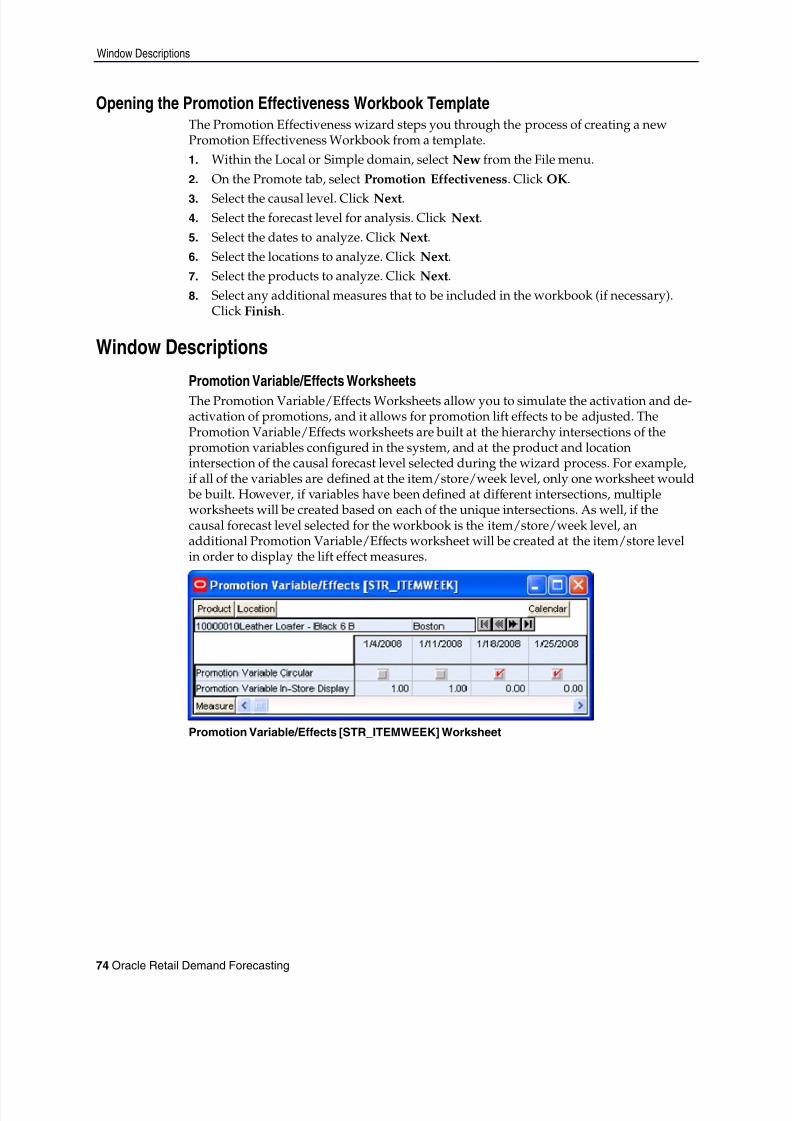
8/10/2019 RDF User Guide
http://slidepdf.com/reader/full/rdf-user-guide 84/120
Window Descriptions
74 Oracle Retail Demand Forecasting
Opening the Promotion Effectiveness Workbook TemplateThe Promotion Effectiveness wizard steps you through the process of creating a newPromotion Effectiveness Workbook from a template.1. Within the Local or Simple domain, select New from the File menu.2. On the Promote tab, select Promotion Effectiveness . Click OK .3. Select the causal level. Click Next .4. Select the forecast level for analysis. Click Next .5. Select the dates to analyze. Click Next .6. Select the locations to analyze. Click Next .7. Select the products to analyze. Click Next .8. Select any additional measures that to be included in the workbook (if necessary).
Click Finish .
Window DescriptionsPromotion Variable/Effects WorksheetsThe Promotion Variable/Effects Worksheets allow you to simulate the activation and de-activation of promotions, and it allows for promotion lift effects to be adjusted. ThePromotion Variable/Effects worksheets are built at the hierarchy intersections of thepromotion variables configured in the system, and at the product and locationintersection of the causal forecast level selected during the wizard process. For example,if all of the variables are defined at the item/store/week level, only one worksheet would
be built. However, if variables have been defined at different intersections, multipleworksheets will be created based on each of the unique intersections. As well, if thecausal forecast level selected for the workbook is the item/store/week level, anadditional Promotion Variable/Effects worksheet will be created at the item/store levelin order to display the lift effect measures.
Promotion Variable/Effects [STR_ITEMWEEK] Worksheet
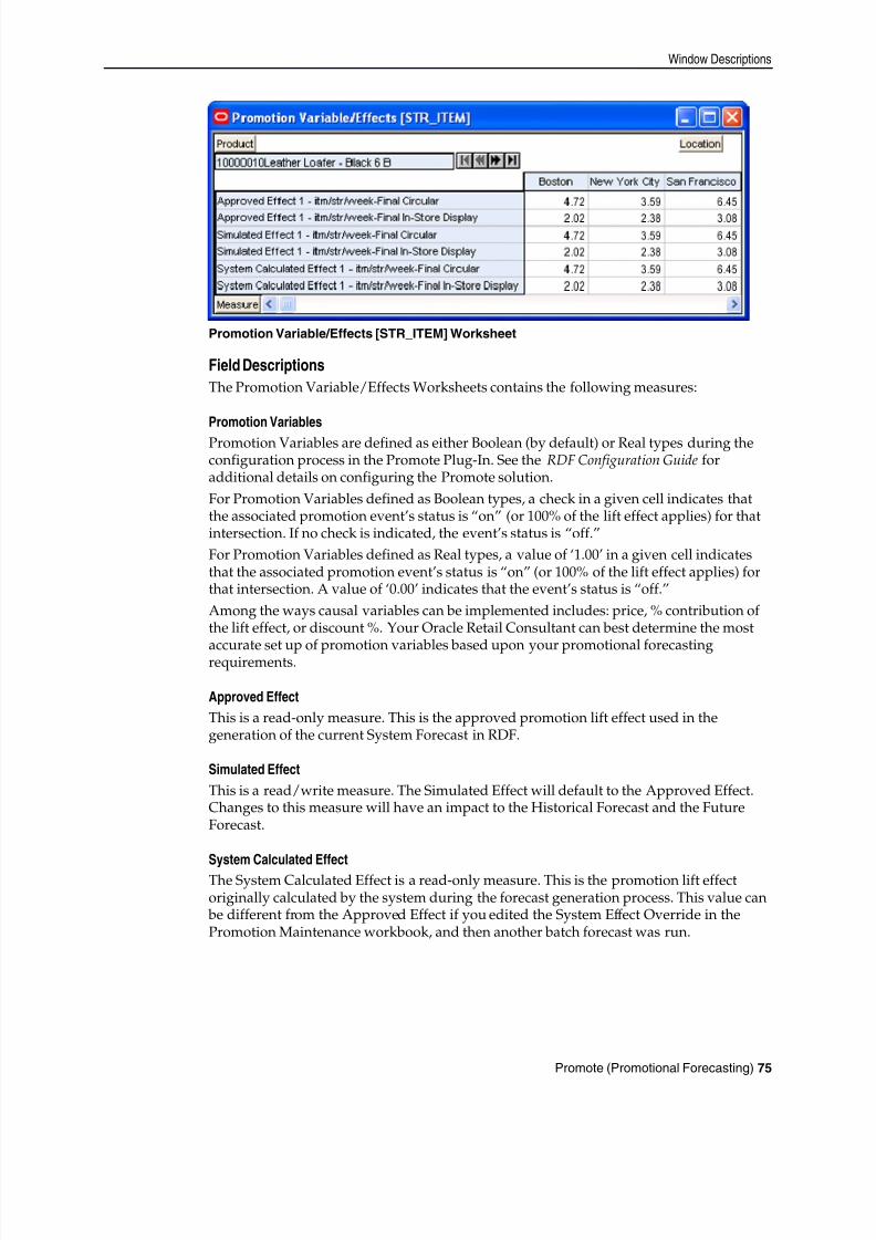
8/10/2019 RDF User Guide
http://slidepdf.com/reader/full/rdf-user-guide 85/120
Window Descriptions
Promote (Promotional Forecasting) 75
Promotion Variable/Effects [STR_ITEM] Worksheet
Field DescriptionsThe Promotion Variable/Effects Worksheets contains the following measures:
Promotion VariablesPromotion Variables are defined as either Boolean (by default) or Real types during theconfiguration process in the Promote Plug-In. See the RDF Configuration Guide foradditional details on configuring the Promote solution.For Promotion Variables defined as Boolean types, a check in a given cell indicates thatthe associated promotion event’s status is “on” (or 100% of the lift effect applies) for thatintersection. If no check is indicated, the event’s status is “off.”For Promotion Variables defined as Real types, a value of ‘1.00’ in a given cell indicatesthat the associated promotion event’s status is “on” (or 100% of the lift effect applies) forthat intersection. A value of ‘0.00’ indicates that the event’s status is “off.”Among the ways causal variables can be implemented includes: price, % contribution ofthe lift effect, or discount %. Your Oracle Retail Consultant can best determine the most
accurate set up of promotion variables based upon your promotional forecastingrequirements.
Approved EffectThis is a read-only measure. This is the approved promotion lift effect used in thegeneration of the current System Forecast in RDF.
Simulated EffectThis is a read/write measure. The Simulated Effect will default to the Approved Effect.Changes to this measure will have an impact to the Historical Forecast and the FutureForecast.
System Calculated EffectThe System Calculated Effect is a read-only measure. This is the promotion lift effectoriginally calculated by the system during the forecast generation process. This value can
be different from the Approved Effect if you edited the System Effect Override in thePromotion Maintenance workbook, and then another batch forecast was run.
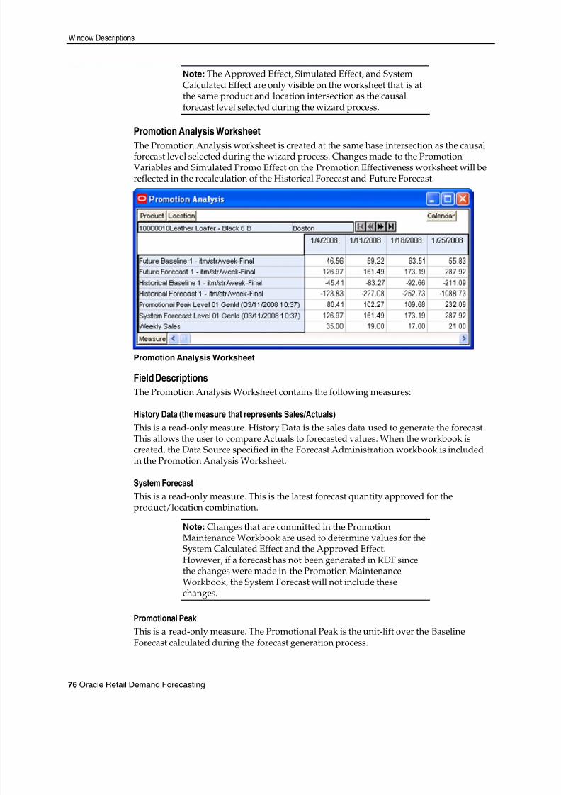
8/10/2019 RDF User Guide
http://slidepdf.com/reader/full/rdf-user-guide 86/120
Window Descriptions
76 Oracle Retail Demand Forecasting
Note: The Approved Effect, Simulated Effect, and SystemCalculated Effect are only visible on the worksheet that is atthe same product and location intersection as the causalforecast level selected during the wizard process.
Promotion Analysis WorksheetThe Promotion Analysis worksheet is created at the same base intersection as the causalforecast level selected during the wizard process. Changes made to the PromotionVariables and Simulated Promo Effect on the Promotion Effectiveness worksheet will bereflected in the recalculation of the Historical Forecast and Future Forecast.
Promotion Analysis Worksheet
Field DescriptionsThe Promotion Analysis Worksheet contains the following measures:
History Data (the measure that represents Sales/Actuals)This is a read-only measure. History Data is the sales data used to generate the forecast.This allows the user to compare Actuals to forecasted values. When the workbook iscreated, the Data Source specified in the Forecast Administration workbook is includedin the Promotion Analysis Worksheet.
System ForecastThis is a read-only measure. This is the latest forecast quantity approved for theproduct/location combination.
Note: Changes that are committed in the PromotionMaintenance Workbook are used to determine values for theSystem Calculated Effect and the Approved Effect.However, if a forecast has not been generated in RDF sincethe changes were made in the Promotion MaintenanceWorkbook, the System Forecast will not include thesechanges.
Promotional PeakThis is a read-only measure. The Promotional Peak is the unit-lift over the BaselineForecast calculated during the forecast generation process.
8/10/2019 RDF User Guide
http://slidepdf.com/reader/full/rdf-user-guide 87/120
Procedures in Promotional Forecasting
Promote (Promotional Forecasting) 77
Future BaselineThis is a read-only measure. Calculated as the System Forecast minus (–) the PromotionalPeaks. User-changes to the editable measures in the Promotion Variable/Effectsworksheets do not affect this value.
Future Forecast
This is a read-only measure. The Future Forecast equals the Future Baseline multiplied by the Simulated Effect if the promotion variable is greater than 0 (zero). If there aremore than one promotion variables, the sum of the Simulated Effects for the variables ismultiplied by the Future Baseline.If there is no active promotion variable, the Future Forecast equals the Future Baseline.
Historical BaselineThis is a read-only measure. Calculated in one of two ways based on the value of theSystem Forecast:1. Historical Baseline equals Sales minus the Promotion Peak if the System Forecast is
greater than 0 (zero).
2.
Historical Baseline equals Sales with the Moving Average applied if the SystemForecast equals 0 (zero). If Sales are also 0 (zero), the Historical Baseline will alsoequal 0 (zero).
Historical ForecastThis is a read-only measure. The Historical Forecast equals the Historical Baselinemultiplied by the Simulated Effect if the promotion variable is greater than 0 (zero). Ifthere are more than one promotion variables, the sum of the Simulated Effects for thevariables is multiplied by the Historical Baseline.If there is no active promotion variable, the Historical Forecast equals the HistoricalBaseline.
Procedures in Promotional ForecastingThe following outlines the standard procedures performed in order to set up the systemto run a promotional forecast (more detailed steps follow in the next section): Set up the system to run a promotional forecast Set forecast parameters in the Forecast Administration Workbook Set forecast parameters in the Forecast Maintenance Workbook Set promotions to be active in the Promotion Planner Workbook Run the batch forecast View and Edit Causal Forecast results Analyze forecasts in the Forecast Approval Workbook
Analyze and edit causal effects in the Promotion Maintenance Workbook Promotion Simulation (what-ifing) and Analysis
8/10/2019 RDF User Guide
http://slidepdf.com/reader/full/rdf-user-guide 88/120
Procedures in Promotional Forecasting
78 Oracle Retail Demand Forecasting
Setting Up the System to Run a Promotional Forecast1. On the Forecast tab, select and build a Forecast Administration Workbook.
a. In the Forecast Administration Workbook: Advance Parameter Worksheet, selectGenerate Baseline .
b. Optional: Set the Default Forecast Method to Causal for the desired level if the
level is to be use only for Promotional Forecasting.c. Optional: Set the Causal Higher Intersection for the desired level if the Override
from Higher Level promotion type will be used.d. Optional for use with Daily Causal Forecasting: Set the values for the following
parameters: – Causal Aggregation Profile – Causal Calculation Intersection – Causal Calculation Intersection Periodicity
e. Commit your changes to the master database by selecting Commit Now from theFile menu.
2. On the Forecast tab, select and build a Forecast Maintenance Workbook.a. Set the Forecast Method Override to Causal for any items/locations at the
desired levels that will use Promotional Forecasting.b. Commit your changes to the master database by selecting Commit Now from the
File menu.3. On the Forecast tab, select and build a Promotion Planner Workbook.
a. Set causal variables for items and locations historically in that the selectedpromotions are active.
b. Commit your changes to the master database by selecting Commit Now from theFile menu.
4. On the Forecast tab, select Run Batch . Generate a Forecast.
Viewing a Forecast that Includes Promotion Effects1. On the Forecast tab, select and build a Forecast Approval Workbook and include
System Baseline in your workbook.2. In the Final Level Worksheet review the System Baseline and the System Forecast.
The System Baseline is predicted demand given no causal effects. The SystemForecast is the sum of the System Baseline and the Promotional Peak calculatedduring the forecast generation process based on the causal data and settings.
8/10/2019 RDF User Guide
http://slidepdf.com/reader/full/rdf-user-guide 89/120
Procedures in Promotional Forecasting
Promote (Promotional Forecasting) 79
Viewing and Editing Promotion System-Calculated Effects1. On the Promote tab, select and build a Promotion Maintenance Workbook.
a. In the PromoEffects Worksheet review the System-Calculated Effect.b. If the System Calculated Effect is to be modeled using a method other than
Automatic, edit the Promotion Effect Type .c. If you choose to adjust the system-calculated effect, adjustments can be made to
the System Effect Override. You must also set the Promotion Effect Type toOverride All or Override Future Only .
2. On the Forecast tab, select Run Batch . Generate a Forecast.
Promotion Simulation (“what-if?”) and AnalysisFollow this procedure to perform analysis on past promotions and simulate the effects ofhistoric or future promotions:1. On the Promote tab, select and build a Promotion Effectiveness Workbook2. In the Promotion Variable/Effects Worksheet review the Promotion System-
Calculated Effect and edit the Simulated Promo Effect, then select Calculate torecalculate the Future Forecast.
Note: Changes to the Promotion Effects Workbook cannot becommitted; however, this workbook is useful for:
- Reporting on the performance of past promotions.
- Simulating the effects of future promotions to supportmore accurate promotional modeling.

8/10/2019 RDF User Guide
http://slidepdf.com/reader/full/rdf-user-guide 90/120
8/10/2019 RDF User Guide
http://slidepdf.com/reader/full/rdf-user-guide 91/120
Oracle Retail Demand Forecasting Methods 81
6Oracle Retail Demand Forecasting Methods
This chapter discusses the forecasting methods used in Oracle Retail Demand Forecastingin detail.
Forecasting Techniques Used in RDFOracle Retail Demand Forecasting uses a variety of predictive techniques to generateforecasts of demand. The technical methods used are driven by the goal to provide themost accurate forecasts possible in an automatic and efficient manner. These methodshave been analyzed, optimized, and refined over years of research on retail specific data.The primary techniques RDF uses include: Exponential smoothing Regression analysis
Bayesian analysis Prediction intervals Automatic method selection Source level forecasting Promotional forecasting
Exponential SmoothingExponential smoothing models fit basic features of the demand pattern such as level,trend, and seasonality, and project these into the future. These models providecomputational benefits and have been chosen for their ability to handle different types oftime series, including short and/or noisy series that are characteristic of retail sales. They
are "smoothing" models because they use weighted averages on historic data. They are"exponential smoothing" models because the weighting used decays at an exponentialrate. That is, more recent data is weighted more heavily than the past.
Regression AnalysisRegression analysis is another standard technique used in prediction. Regression uses aleast-squares estimator to fit a model of predictor variables to another set of targetvariables. Seasonal Regression is an Oracle Retail specific extension of this procedure foruse in seasonal models with between one and two years of history. Causal Forecastinguses stepwise regression to determine which causal variables are significant.
Bayesian AnalysisBayesian analysis considers a priori information as a starting point in development of aprediction. Bayesian forecasting, as developed by Oracle Retail, uses a sales plan as thestarting point that is adjusted based on observed data. This method fills a gap instandard time series forecasting when new, short lifecycle, or products with significantlifecycles are being forecast.

8/10/2019 RDF User Guide
http://slidepdf.com/reader/full/rdf-user-guide 92/120
Forecasting Techniques Used in RDF
82 Oracle Retail Demand Forecasting
Prediction IntervalsPrediction from these various models gives the estimated mean outcome. By usingstandard statistical distributional assumptions, RDF develops measures of uncertaintyassociated with forecast point estimates from these models. While this is of key concernfor various optimization solutions of the forecast, the technical details are beyond thescope of this document. For further details on prediction interval calculations, seeChar&Yatfield, International Journal of Forecasting, March 1992.
Automatic Method SelectionProviding multiple forecasting methods is only valuable if the appropriate model can beselected in an accurate and efficient manner. In order to make this feasible in a retailenvironment, Oracle Retail has developed a number of different Meta-Methods that canautomatically select the best method among a number of competing models. AutomaticExponential Smoothing (AutoES) is an example of one such method that clients canselect. The final selection between the competing models is made according to aperformance criterion that involves a tradeoff between the model’s fit over the historicdata and its complexity. A description of the competing models used within AutoES isdescribed in section two of this document. In academia, this discipline is known as Information Theory and is used in the combination and selection of various competingmodels.
Source Level ForecastingSometimes it is difficult to capture seasonality, trend, or causal effects on the final level(item/Store) due to scarcity of the data. Also, time series are often too noisy at that level.To overcome these issues, RDF utilizes source level forecasting. In source levelforecasting, data is aggregated first to a higher level across the product or locationhierarchy (or both). Then the forecast is generated and proportionally spread down to thefinal level. We have experimentally proven that source level forecasting technique oftenimproves the accuracy on the final level.
Promotional ForecastingIn some instances, especially in retail, pure time series techniques are inadequate forforecasting demand. Instead of using only historic demand patterns to forecast futuredemand, additional causal or promotional factors are used to better explain pastperformance. With the help of a promotional calendar, an indication of when promotionswill be run in the future, these promotional forecasting techniques can better predictdemand in the future.
8/10/2019 RDF User Guide
http://slidepdf.com/reader/full/rdf-user-guide 93/120
Time Series (Statistical) Forecasting Methods
Oracle Retail Demand Forecasting Methods 83
Time Series (Statistical) Forecasting MethodsThis section describes those techniques within RDF that generate forecasts directly fromonly a single time series. Generally the time series provided is past sales history for agiven item/Store that is used to predict what future demand might be. In actual practicethese algorithms have been and can be used to forecast a myriad of different data streams
at any product/location level (shipment data at item/warehouse, financial data atdept./chain, and so on).The following topics present fundamentals of the Oracle Retail Demand Forecastingstatistical forecasting processes. Included is a discussion of the importance of confidenceintervals and confidence limits, the time series methods used to generate forecasts, andhow the best forecasting method is selected from a list of candidate models.A wide variety of statistical forecasting techniques are available, ranging from verysimple to very sophisticated. All of these methods attempt to best capture the statisticalprobability distribution discussed above, and they do this by fitting quantitative modelsto statistical patterns from historical data. Put simply, the better the history of thevariable being forecasted, the stronger these statistical patterns will be. Increased forecastaccuracy depends on the strength of these patterns in relation to background
irregularities.Oracle Retail Demand Forecasting is able to use several time series methods to produceforecasts. Time series methods extrapolate features from the past (in this case, past salesdata) to the future. The time series methods that the system offers include: Auto Exponential Smoothing Forecasting (AutoES) Seasonal Exponential Smoothing Forecasting (SeasonalES) Simple Moving Average Simple Exponential Smoothing Croston’s Method Holt Exponential Smoothing Multiplicative Winters Exponential Smoothing
Additive Winters Exponential Smoothing Seasonal Regression Bayesian Information Criterion
Why Use Statistical Forecasting?The purpose of statistical forecasting is to make the process of predicting future events
both objective and quantitative. Statistical forecasting utilizes information from the past(such as sales data) to predict what will happen in the future. Forecast accuracy dependson the degree to which a mathematical model can detect and extract statistical patternsfrom historic data. The most common statistical methodologies used are univariate. Thismeans that they are based solely on the history of one variable, such as sales. Each
forecast observation reflects a future value of the sole input variable. Statisticalforecasting processes are relatively easy to implement, and the better the historical data,the better the resulting forecasts.Businesses benefit greatly from the use of systematic statistical forecasting techniquesthat aim to accurately predict product demand, enabling these businesses to maintainsufficient product inventory levels. When inventory levels are optimized, lost sales dueto product stock-outs are greatly reduced, as are the costs incurred by overstocking.

8/10/2019 RDF User Guide
http://slidepdf.com/reader/full/rdf-user-guide 94/120
Time Series (Statistical) Forecasting Methods
84 Oracle Retail Demand Forecasting
Exponential Smoothing (ES) Forecasting MethodsThe primary process by which RDF automatically fits an exponential smoothing model toa time series is called Automatic Exponential Smoothing (AutoES). When AutoESforecasting is chosen in RDF, a collection of candidate models is initially considered. Themodels in the candidate list include:
Simple (One Parameter) Exponential Smoothing Croston’s Method (Intermittent ES) Holt (Two Parameter) Exponential Smoothing (Trend ES) Winters (Three Parameter) Exponential Smoothing (Seasonal ES) Seasonal Regression
These models include level information, level and trend information, and level, trend andseasonality information, respectively. The optimal smoothing parameters for each modelform are determined automatically (that is, greater smoothing will be applied to noisierdata). The final selection between the resulting models is made according to aperformance criterion that involves a tradeoff between the model’s fit over the historicdata and its complexity.
The amount of available historic information can affect the complexity of the model thatcan be fit. For example, fitting a seasonal model would not be appropriate without acomplete year of historic data. In fact, one prefers to see each “season” occur multipletimes. For a particular series, even if the amount of available history allows one to fit acomplex model (that is, one with seasonal components), the resulting model is notnecessarily superior to a simpler model. If a simpler model (for example, a model withonly a level component or level and trend components) fits “as well” as a seasonalmodel, the AutoES forecasting process will find the simpler model to be preferable. Insuch a case, the simpler model captures the basic features supported by the data withoutover fitting and therefore will generally project better forecasts.
AverageA simple moving average forecast involves taking the average of the past n time periodsand using that average as the forecast for all future time periods (where n is the length offitting period). Simple moving average forecasts are frequently used in the system
because: They make few assumptions about the historical time series They can be generated with little historical data They are very fast to generate
Typically, moving average forecasts are generated at the final forecast level (for example,item/Store) and their results used to spread more sophisticated higher-level forecasts (forexample, those generated with exponential smoothing).A Simple Moving Average model assumes that historical data is too short or noisy toconsider seasonal effects or local trend, and is based on the level of the series. Since thismodel does not use a smoothing parameter to place added weight on more recenthistoric values, a Simple Moving Average model is not actually in the exponentialsmoothing family. However, it is an adequate model to use when low-level (finalforecast) ratios are needed for RDF’s spreading of high-level (aggregate) forecasts. Thatis, when aggregate forecasts can be calculated for long and less noisy aggregate timeseries, Simple Moving Average models provide an adequate (and computationally quick)forecast to determine the ratios needed for RDF spreading. User input in overriding theautomatic training horizon further enhances the simple robustness of this model for base-level data.

8/10/2019 RDF User Guide
http://slidepdf.com/reader/full/rdf-user-guide 95/120
Time Series (Statistical) Forecasting Methods
Oracle Retail Demand Forecasting Methods 85
Simple Exponential SmoothingSimple Exponential Smoothing does not consider seasonality or trend features in thedemand data (if they exist). It is the simplest model of the exponential smoothing family,yet still adequate for many types of RDF demand data. Forecasts for short horizons can
be estimated with Simple Exponential Smoothing when less than a year of historicdemand data is available and acts-like associations are not assigned in RDF.The following figure is an example of a forecast in which data seems to be un-trendedand un-seasonal; note the flat appearance of the forecast.
Croston’s MethodCroston’s method is used when the input series contains a large number of zero datapoints (that is, intermittent demand data). The method involves splitting the originaltime series into two new series: (i) magnitude series and (ii) frequency series. Themagnitude series contains all the non-zero data points, while the frequency seriesconsists of the time intervals between consecutive non-zero data points. A SimpleExponential Smoothing model is then applied to each of these newly created series toforecast a magnitude level as well as a frequency level. The ratio of the magnitudeestimate over the frequency estimate is the forecast level reported for the original series.The following figure shows a sales history of data where the demand for a given periodis often zero.
Simple/Intermittent Exponential SmoothingThis method is a combination of the Simple ES and Croston’s (Intermittent ES) methods.The Simple ES model is applied to the time series unless a large number of zero datapoints are present. In this case, the Croston’s model is applied.
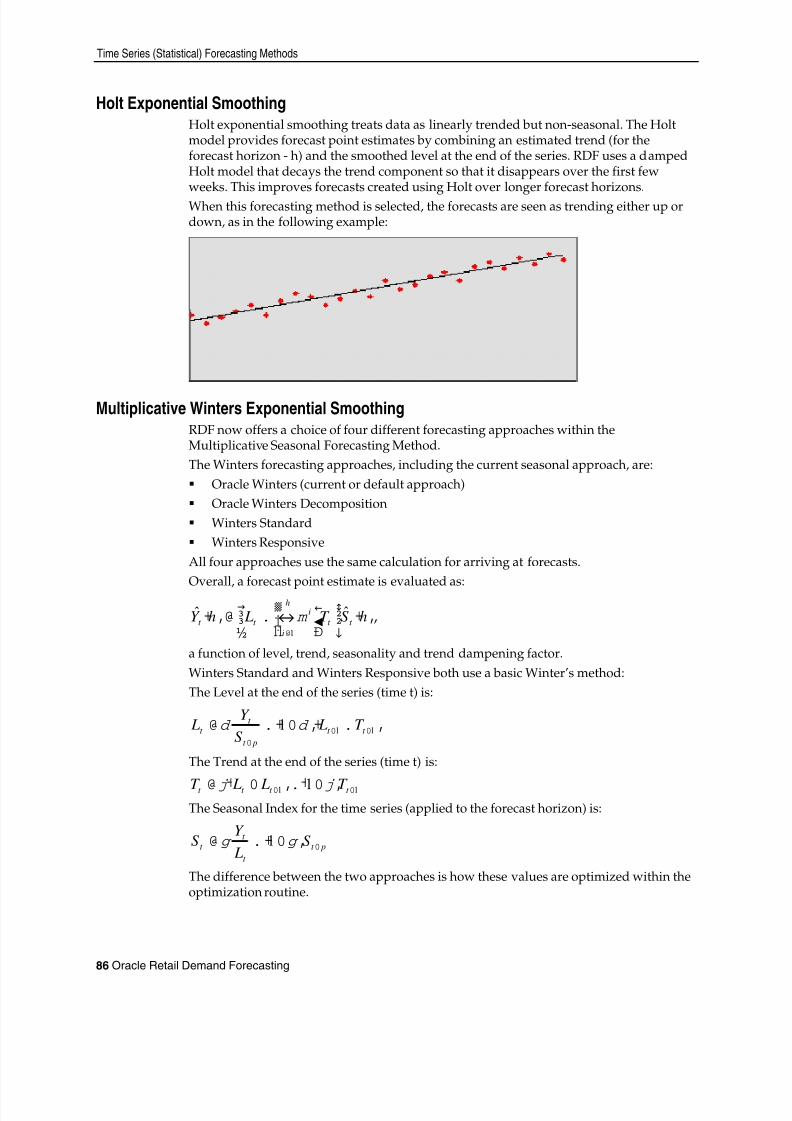
8/10/2019 RDF User Guide
http://slidepdf.com/reader/full/rdf-user-guide 96/120
Time Series (Statistical) Forecasting Methods
86 Oracle Retail Demand Forecasting
Holt Exponential SmoothingHolt exponential smoothing treats data as linearly trended but non-seasonal. The Holtmodel provides forecast point estimates by combining an estimated trend (for theforecast horizon - h) and the smoothed level at the end of the series. RDF uses a dampedHolt model that decays the trend component so that it disappears over the first fewweeks. This improves forecasts created using Holt over longer forecast horizons.When this forecasting method is selected, the forecasts are seen as trending either up ordown, as in the following example:
Multiplicative Winters Exponential SmoothingRDF now offers a choice of four different forecasting approaches within theMultiplicative Seasonal Forecasting Method.The Winters forecasting approaches, including the current seasonal approach, are: Oracle Winters (current or default approach) Oracle Winters Decomposition Winters Standard Winters Responsive
All four approaches use the same calculation for arriving at forecasts.Overall, a forecast point estimate is evaluated as:
( ) ( )hS T LhY t t
h
i
it t
ˆˆ
1 += ∑
=
ϕ ,
a function of level, trend, seasonality and trend dampening factor.Winters Standard and Winters Responsive both use a basic Winter’s method:The Level at the end of the series (time t) is:
( )( ) 111
−−−
+−+= t t pt
t t T L
S
Y L α α
The Trend at the end of the series (time t) is:
) ) 11 1 −− −+−= t t t t T L LT γ γ The Seasonal Index for the time series (applied to the forecast horizon) is:
( ) pt t
t t S
L
Y S −−+= δ δ 1
The difference between the two approaches is how these values are optimized within theoptimization routine.
8/10/2019 RDF User Guide
http://slidepdf.com/reader/full/rdf-user-guide 97/120
Time Series (Statistical) Forecasting Methods
Oracle Retail Demand Forecasting Methods 87
Oracle Winters and Oracle Winters Decomposition use a Winters-based decompositionapproach to update the level, trend and Seasonal Indexes. Each of these methodscalculates initial seasonal indices from a baseline Holt forecast. Seasonal indices, leveland trend are then updated in separate stages, using Winter’s model as a basis for theupdates. The difference between the two approaches is which parameters are optimizedand in which stages seasonal indices are updated.
Oracle WintersOracle Winters is the current seasonal forecasting approach, which uses a combination ofWinters approach and decomposition. Decomposition allows level and trend to beoptimized independently while maintaining a seasonal curve.From sufficient data, RDF extracts seasonal indexes that are assumed to havemultiplicative effects on the de-seasonalized series. Note that the component describing
the de-seasonalized values (which is multiplied by the seasonal index)hS t
ˆ) is the Holt
model described above. In this case, three parameters are used to control smoothing ofthe components of level, trend, and seasonality.
Oracle Winters DecompositionLike the Oracle Winters seasonal forecasting approach, Oracle Winters Decompositionuses a combination of Winters approach and decomposition.From sufficient data, RDF extracts seasonal indexes that are assumed to havemultiplicative effects on the de-seasonalized series. Note that the component describing
the de-seasonalized values (which is multiplied by the seasonal index)hS t
ˆ) is the Holt
model described above.The key difference between Oracle Winters and Oracle Decomposition is that theSeasonal smoothing parameter is also optimized, and the calculation of Seasonal Indicesand de-seasonalizing of data is done with in the optimization routine for Oracle WintersDecomposition.
Also the optimization routine with in Oracle Winters Decomposition, while minimizingforecast errors, tends to weigh more recent Forecast errors heavier.As with Oracle Winters, three parameters are used to control smoothing of level, trend,and seasonality.Key differences between Oracle Winters and Oracle Winters Decomposition include: Seasonal smoothing factor is optimized. The optimization places more importance on recent sales than historical sales. Seasonal indices are recalculated based on optimization.
When this forecasting approach is selected, the forecasts tend to be more responsive torecent changes in levels while maintaining a substantial seasonal component.

8/10/2019 RDF User Guide
http://slidepdf.com/reader/full/rdf-user-guide 98/120
Time Series (Statistical) Forecasting Methods
88 Oracle Retail Demand Forecasting
Winters StandardThe Winters Standard uses a standard Winters model, with no additional calculations.All three smoothing parameters are optimized here.Initial Seasonal Indices are set to one. Initial level and trend are calculated from averageselling levels over initial periods. The optimization routine chooses optimal level, trendand smoothing parameters that minimize Forecast Errors in the fit region. All forecasterrors within the fit region are weighed equally.Seasonal Indices, level and trend are calculated based on the optimal values of level,trend, and Seasonal Smoothing parameters: α, γ and δ. When this forecasting approach is selected, the forecasts tend to be responsive to changesin levels. In cases where there is no obvious correlation in seasonality from period toperiod or where there are significant changes in level, these forecasts may generatesmoother, less seasonal forecasts.
Winters ResponsiveWinters Responsive is similar to Winters Standard except the Optimization routine,while minimizing forecast errors, weighs more recent Forecast errors heavier. Winters
Responsive, like Standard Winters, optimizes all three smoothing parameters.When this forecasting approach is selected, the forecasts tend to be more responsive torecent changes in levels. In cases where there are significant shift in levels, resulting inhigh responsiveness to levels, these forecasts tend to be smoother, with less seasonality.When the Multiplicative Seasonal forecasting method is selected, the forecasts tend tolook “squiggly, as shown in the following figure.
Multiplicative Winters Exponential Smoothing
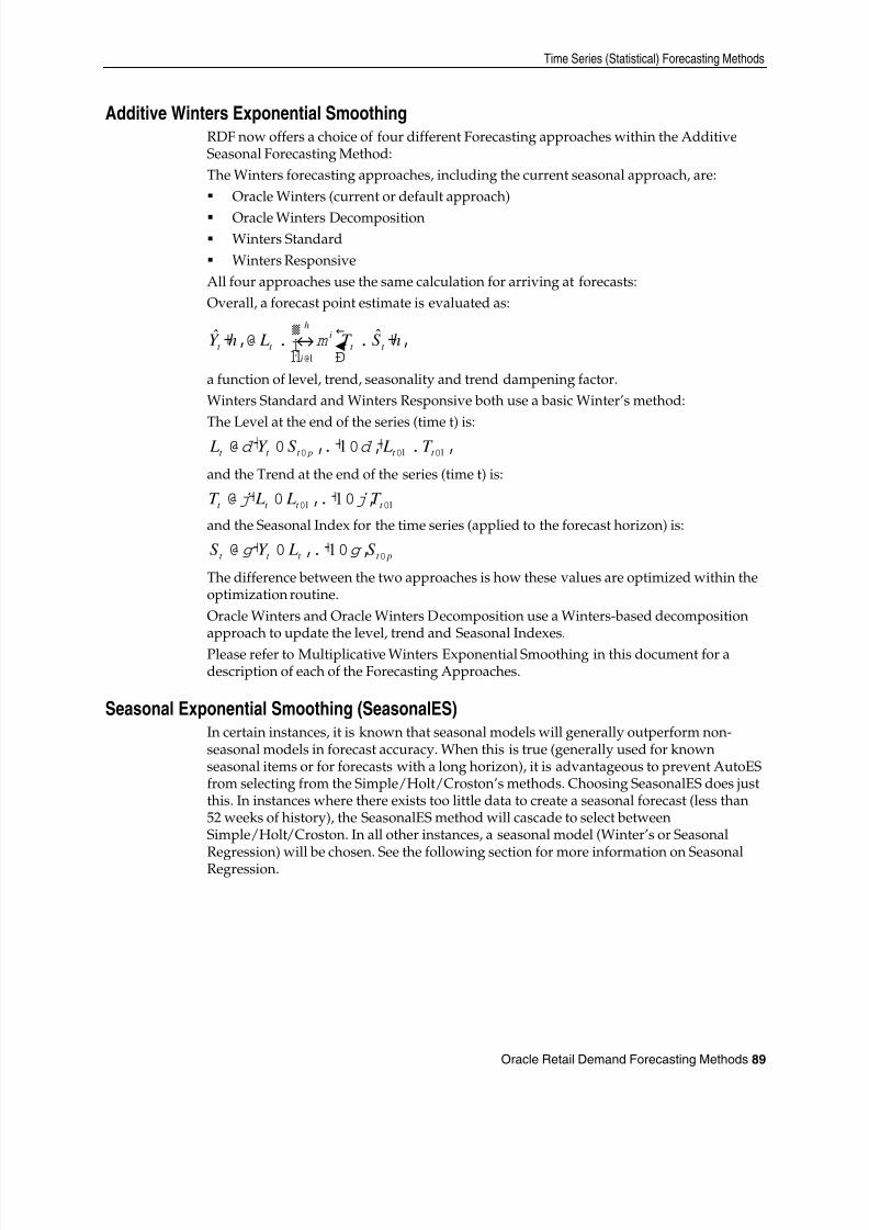
8/10/2019 RDF User Guide
http://slidepdf.com/reader/full/rdf-user-guide 99/120
Time Series (Statistical) Forecasting Methods
Oracle Retail Demand Forecasting Methods 89
Additive Winters Exponential SmoothingRDF now offers a choice of four different Forecasting approaches within the AdditiveSeasonal Forecasting Method:The Winters forecasting approaches, including the current seasonal approach, are: Oracle Winters (current or default approach)
Oracle Winters Decomposition Winters Standard Winters Responsive
All four approaches use the same calculation for arriving at forecasts:Overall, a forecast point estimate is evaluated as:
( ) ( ) hS T LhY t t
h
i
it t
ˆˆ
1
++= ∑ =
ϕ
a function of level, trend, seasonality and trend dampening factor.Winters Standard and Winters Responsive both use a basic Winter’s method:The Level at the end of the series (time t) is:
) ) )111
−−− +−+−= t t pt t t T LS Y L α α
and the Trend at the end of the series (time t) is:
) ) 111
−− −+−= t t t t T L LT γ γ
and the Seasonal Index for the time series (applied to the forecast horizon) is:
) ) pt t t t S LY S −−+−= δ δ 1
The difference between the two approaches is how these values are optimized within theoptimization routine.Oracle Winters and Oracle Winters Decomposition use a Winters-based decompositionapproach to update the level, trend and Seasonal Indexes.Please refer to Multiplicative Winters Exponential Smoothing in this document for adescription of each of the Forecasting Approaches.
Seasonal Exponential Smoothing (SeasonalES)In certain instances, it is known that seasonal models will generally outperform non-seasonal models in forecast accuracy. When this is true (generally used for knownseasonal items or for forecasts with a long horizon), it is advantageous to prevent AutoESfrom selecting from the Simple/Holt/Croston’s methods. Choosing SeasonalES does justthis. In instances where there exists too little data to create a seasonal forecast (less than52 weeks of history), the SeasonalES method will cascade to select betweenSimple/Holt/Croston. In all other instances, a seasonal model (Winter’s or SeasonalRegression) will be chosen. See the following section for more information on SeasonalRegression.
8/10/2019 RDF User Guide
http://slidepdf.com/reader/full/rdf-user-guide 100/120
Time Series (Statistical) Forecasting Methods
90 Oracle Retail Demand Forecasting
Seasonal RegressionA common benchmark in seasonal forecasting methods is sales last year. A sales last yearforecast is based entirely on sales from the same time period of last year. Forecastingusing only sales last year involves simple calculations and often outperforms other moresophisticated seasonal forecasting models. This method performs best when dealing withhighly seasonal sales data with a relatively short sales history.The seasonal models used in earlier releases of Oracle Retail Demand Forecasting(Additive and Multiplicative Winters) were designed to determine seasonality. However,they were not designed to work with sales histories of shorter than two years. Becausesales histories of longer than two years are often difficult to obtain, many retailenvironments need a seasonal forecast that can accommodate sales data histories of
between one and two years. In addition, the Additive and Multiplicative Winters modelssearch for short-term trends and have difficulties with trends occurring inside theseasonal indices themselves. The current Oracle Retail Demand Forecasting SeasonalRegression forecasting model is designed to address these needs.The Seasonal Regression Model uses simple linear regression with last year's data as thepredictor variable and this year's sales as the target variable. The system determines themultiplicative and additive weights that best fit the data on hand. When optimizing theSeasonal Regression Model, the sales last year forecast is inherently considered, and itwill automatically be used if it is the model that best fits the data. If there have beensignificant shifts in the level of sales from one year to the next, the model will learn thatshift and appropriately weight last year's data (keeping the same shape from last year,
but adjusting its scale).As with other seasonal models, you can forecast demand for products with insufficientsales histories using this method if: You paste in fake history as needed, providing a seasonal profile for the previous
year. You also forecast for a source level (with the same seasonality profile as the
forecasted item and with more than one year of history) using seasonal regressionand spread these forecast results down to the member products.
The Seasonal Regression Model is included in the AutoES family of forecasting models,and is thus a candidate model that will be selected if it best fits the data.This method captures the trend of a series through the slope of the regression line whilethe series shifted by a cycle provides its seasonal profile. Using this method, the resultingforecast for the original series is calculated. The regression method provides a much
better forecast of the series than was possible with the other exponential smoothingalgorithms.Based on the assumptions of the model that this method is trying to describe, versus thenoisy data it is likely to receive, several exceptions to this regression technique are caughtand corrected. First, since it is logically impossible to receive a negative value for theslope (such a value suggesting an inverse seasonality), whenever a negative slope isdetected, the regression is rerun with the intercept fixed to zero. This guarantees that apositive slope will be calculated and thus a more logical forecast will be given.The second noise-driven concession is to check the slope to determine if it is either tooslight or too great. If this is the case, the method rejects itself out of hand and allows oneof the other competing methods to provide the forecast.
Bayesian Information Criterion (BIC)Within AutoES, the model that minimizes the Bayesian Information Criterion (BIC) isselected as the final model. The BIC criterion attempts to balance model complexity with
8/10/2019 RDF User Guide
http://slidepdf.com/reader/full/rdf-user-guide 101/120
Time Series (Statistical) Forecasting Methods
Oracle Retail Demand Forecasting Methods 91
goodness-of-fit over the historical data. The BIC criterion rewards a model for goodness-of-fit and penalizes a model for its complexity. The complexity penalty is necessary toavoid over fitting.There are various equivalent versions of the Bayesian Information Criterion, but RDFminimizes the following:
n
k
ns BIC 2
⋅= where n is the number of periods in the available data history, k is the number ofparameters to be estimated in the model (a measure of model complexity), and s is theroot mean squared error computed with one-step-ahead forecast errors resulting fromthe fitted model (a measure of goodness-of-fit). Note that since each member of themodel candidate list is actually a family of models, an optimization routine to selectoptimal smoothing parameters is required to minimize s for each model form (that is, toselect the best model).Within RDF, a few modifications to the standard selection criteria have been made. Theseinclude reducing the number of parameters the Winter’s model is penalized bydiscounting seasonal indices that have little impact on the forecast (multiplicative indicesclose to 1, additive indices close to 0). These changes tend to favor the seasonal models to
a slightly higher degree that improves the forecasts on retail data, especially for longerforecast horizons.
AutoES FlowchartThe following outlines the processing routine steps that the system runs through toevaluate each time series set to forecast using the AutoES method.1. Filter all leading zeros in the input data that is within the training window. Go to2. Does the time series contain the minimum data points to qualify to forecast using the
Croston’s method? If yes, generate the forecast and statistics using the Croston’smethod, and move on to the next time series. If no, move on to Step 3.
3. Does the time series contain enough relevant data to generate a forecast? If yes,generate a forecast and statistics using the Simple ES method and move on to Step 4.If no, do not forecast, and go to the next time series.
4. Does the time series contain the minimum data points to qualify to forecast using theHolt method? If yes, generate a forecast and statistics using the Holt method andmove on to Step 5. If no, move on to Step 5.
5. Does the time series contain more than 52 weeks of input data? If yes, generate aforecast and statistics using the Seasonal Regression method and move on to Step 6.If no, move on to Step 9.
6. Does the time series contain the minimum data points to qualify to forecast usingWinters methods? If yes, move on to Step 7. If no, move on to Step 9.
7. Does the time series contain any data point with sales equal qualify to forecast usingAdditive Winters method? If yes, generate the forecast and statistics using the
Additive Winters method, and move on to Step 9. If no, move on to Step 8.8. Does the time series qualify to forecast using the Multiplicative Winters method? Ifyes, generate the forecast and statistics using both the Additive Winters andMultiplicative Winters methods, and move on to Step 9.
9. Compare all candidate forecasts using BIC Criterion.
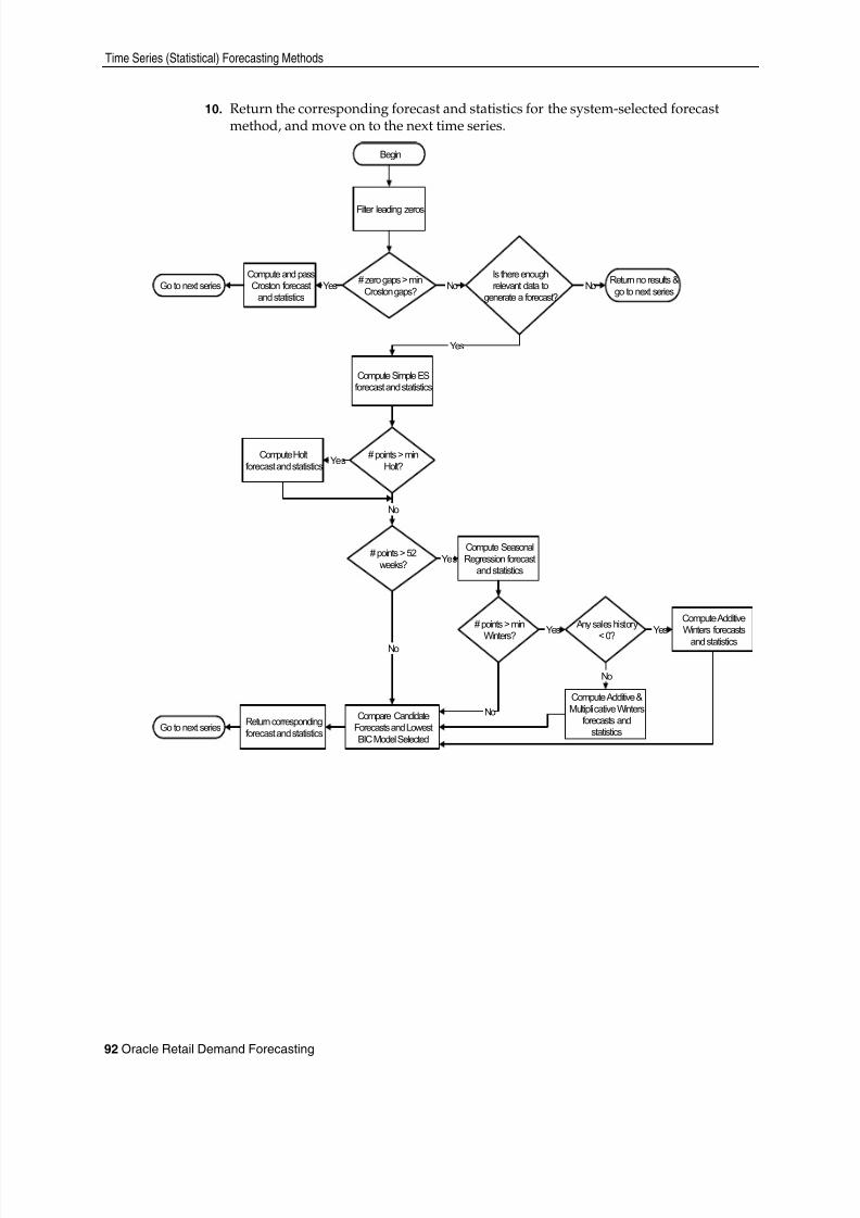
8/10/2019 RDF User Guide
http://slidepdf.com/reader/full/rdf-user-guide 102/120
Time Series (Statistical) Forecasting Methods
92 Oracle Retail Demand Forecasting
10. Return the corresponding forecast and statistics for the system-selected forecastmethod, and move on to the next time series.
Begin
Filter leading zeros
Compute Simple ESforecast and statistics
# zero gaps > minCroston gaps?
Compute and passCroston forecast
and statisticsGo to next series
Compute Holtforecast and statistics
Compare CandidateForecasts and LowestBIC Model Selected
Return correspondingforecast and statisticsGo to next series
Yes
Compute AdditiveWinters forecasts
and statistics
# points > minHolt?
# points > min
Winters?
# points > 52weeks?
Compute SeasonalRegression forecast
and statistics
Is there enoughrelevant data to
generate a forecast?
Any sales history
< 0?
Compute Additive &Multiplicative Winters
forecasts andstatistics
Yes
Yes
No
Yes
No Return no results &go to next seriesNo
Yes
No
Yes
No
No
8/10/2019 RDF User Guide
http://slidepdf.com/reader/full/rdf-user-guide 103/120
Time Series (Statistical) Forecasting Methods
Oracle Retail Demand Forecasting Methods 93
Automatic Forecast Level Selection (Autosource)This section describes how the automatic forecast level selection (Autosource) could helpimprove the accuracy of your forecasts.In the system, one of the key elements to producing accurate forecasts is using thesystem’s ability to aggregate and spread sales data and forecasts across the product andlocation hierarchies. Low selling or relatively new products can use aggregated data fromsimilar products/locations at a higher level in the hierarchy, generate forecasts using thisdata, and then spread these higher level forecasts back down to provide more accurateforecasts. The difficulty comes in deciding which products/locations will benefit fromthis technique and from what level in the hierarchy these source level forecasts should bespread.The Automatic Forecast Level Selection feature of the system automates the selection of
best aggregation level (forecast source level) for each product/location combination.While providing invaluable information regarding the best aggregate level for sourceforecasts, the Automatic Forecast Level Selection process may be very CPU intensive. Tosolve this problem, the task of selecting best aggregation levels for product/locationcombinations is decomposed and processed piecemeal during times when the computerwould normally be idle. Identifying the best aggregation levels for sets of products andlocations can be divided into a number of sub-problems: Forecasting Determining the best source level forecast Status and Scheduling
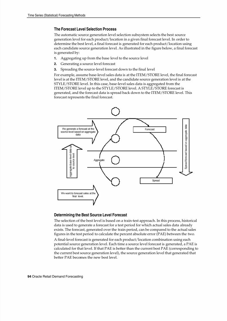
8/10/2019 RDF User Guide
http://slidepdf.com/reader/full/rdf-user-guide 104/120
Time Series (Statistical) Forecasting Methods
94 Oracle Retail Demand Forecasting
The Forecast Level Selection ProcessThe automatic source generation level selection subsystem selects the best sourcegeneration level for each product/location in a given final forecast level. In order todetermine the best level, a final forecast is generated for each product/location usingeach candidate source generation level. As illustrated in the figure below, a final forecastis generated by:1. Aggregating up from the base level to the source level2. Generating a source level forecast3. Spreading the source-level forecast down to the final levelFor example, assume base-level sales data is at the ITEM/STORE level, the final forecastlevel is at the ITEM/STORE level, and the candidate source generation level is at theSTYLE/STORE level. In this case, base-level sales data is aggregated from theITEM/STORE level up to the STYLE/STORE level. A STYLE/STORE forecast isgenerated, and the forecast data is spread back down to the ITEM/STORE level. Thisforecast represents the final forecast.
Determining the Best Source Level ForecastThe selection of the best level is based on a train-test approach. In this process, historicaldata is used to generate a forecast for a test period for which actual sales data alreadyexists. The forecast, generated over the train period, can be compared to the actual salesfigures in the test period to calculate the percent absolute error (PAE) between the two.A final-level forecast is generated for each product/location combination using eachpotential source generation level. Each time a source level forecast is generated, a PAE iscalculated for that level. If that PAE is better than the current best PAE (corresponding tothe current best source generation level), the source generation level that generated that
better PAE becomes the new best level.

8/10/2019 RDF User Guide
http://slidepdf.com/reader/full/rdf-user-guide 105/120
Profile-Based Forecasting
Oracle Retail Demand Forecasting Methods 95
Status and SchedulingIdentifying the best aggregation level for a given set of products and locations may take asignificant amount of time (that is, an amount of time that is greater than the duration ofthe computer’s shortest idle period). This task; however, can be partitioned meaning thatthe problem of selecting the best aggregation levels can be decomposed into smaller subproblems to be solved piecemeal during times when the computer would normally beidle.For each product/location combination at the final forecast level, the problem consists of:1. Generating forecasts at each unique aggregation level2. Using the train-test approach to evaluate the percent absolute error statistics for eachOne or more of these subtasks will be performed during each period that the computer isidle. The best aggregation status keeps track of which sub problems have been performedand which sub problems remain. In this way, when the best aggregation procedure isrun, the procedure knows what the next sub problem is.Best aggregation level procedures are run during idle computer periods. The schedulingof the Automatic Forecast Level Selection process ( Autosource ) must be integrated withthe schedules of other machine processes. In general, you should select a schedule so that
source generation level selection does not conflict with other activities. The following isan example of a typical schedule for the Automatic Forecast Level Selection process:Monday through Thursday, the selection process starts at midnight and runs for eighthours. On Friday and Saturday, the process is allowed to run for 20 hours. Sunday isreserved for generating forecasts.
Using the System-Selected Forecast LevelYou have the option of accepting the system-generated source level selection or manuallyselecting a different source level to be used. The value for the source forecast level can bemanipulated in the Final Level Worksheet of the Forecast Maintenance Workbook. Foreach product/location combination, the best source forecast level identified by OracleRetail Demand Forecasting will appear in the Optimal Source Level measure on thisworksheet. You can enable the use of this level by placing a checkmark in the PickOptimal Level measure for that product/location. The absence of a checkmark in thismeasure causes the system to default to the Default Source Level or the Source LevelOverride value if this has been set by the user.
Profile-Based ForecastingThe Profile-based forecasting method generates a forecast based on a seasonal profile.The profile may be loaded, manually entered, or generated by Curve. It can also becopied from another profile and adjusted.
Forecast MethodThe Profile-based forecasting method proceeds as follows:1. The historical data and the profile are loaded.2. The data are de-seasonalized using the profile and then fed to Simple method.3. The alpha is capped by 0.5.4. The Simple forecast is re-seasonalized using the profiles.
8/10/2019 RDF User Guide
http://slidepdf.com/reader/full/rdf-user-guide 106/120
Bayesian Forecasting
96 Oracle Retail Demand Forecasting
Profile-Based Method and New ItemsThe Profile-based forecasting method can be successfully used to forecast new items. Inorder to do that, we need to have a profile (which can be copied from an item that sharesthe same seasonality) and a number that specifies the de-seasonalized demand (DDvalue). The forecast is calculated using the DD value multiplied by the profile. Theconfidence interval is set to 1/3 of the DD value.If the DD value is used to forecast, the history (if exists) of the product is ignored. Oncewe have enough history (number of data points exceed a global parameter), the forecaststops using the DD value and it defaults to the “normal” Profile Based method.
Bayesian ForecastingThe Bayesian Forecasting method is based on combining historic sales data with salesplan data. It is especially effective for new products with little or no historic sales data.Your sales plan can incorporate expert knowledge in two ways ─ shape and scale. Shape is the selling profile or lifecycle that can be derived from a sales plan. For
example, the shape for certain fashion items might show sales ramping up quicklyfor the first four weeks and then trailing off to nothing over the next eight weeks.
Scale , or magnitude, of a sales plan is the total quantity expected to be sold over theplan's duration.
Bayesian Forecasting assumes that the shape that sales will take is known, but the scale isuncertain. In Bayesian Forecasting, when no sales history is available, the sales forecastfigures are equal to the sales plan figures. At this point, there is no reason to mistrust thesales plan. As point of sale data becomes available, the forecast is adjusted and the scale
becomes a weighted average between the initial plan's scale and the scale reflected byknown sales history. Confidence in the sales plan is controlled by the amount of salesdata on hand and a Bayesian sensitivity constant (Bayesian Alpha), which you can set
between zero and infinity.Unlike standard time series forecasting, which requires only sales history to produce aforecast, Bayesian Forecasting requires a sales plan and sales history (if available).Because of this difference, Bayesian Forecasting is not included in AutoES. You mustselect it manually as a forecasting method in Forecast Administration or ForecastMaintenance.Obtaining accurate short life-cycle product forecasts is very difficult, and standardstatistical time series forecasting models frequently do not offer an adequate solution formany retailers. The following are major problems in automatically developing theseforecasts: The lack of substantial sales history for a product (which especially makes obtaining
seasonal forecasts very difficult) The difficulty of automatically matching a new product to a previous product or
profile
The inability to include planners’ intuition into a forecasting model. For example, theoverall sales level of the product, how quickly the product will take off, how theproduct’s sales will be affected by planned promotions.
Using a Bayesian approach, a short life-cycle forecasting algorithm was developed that begins with a product’s seasonal sales plan (that is developed externally to the system bythe planner). As sales information arrives during the first few days or weeks of theseason, the model generates a forecast by merging the information contained in the salesplan with the information contained in the initial sales data. These forecast updates can
be critical to a company’s success and can be used to increase or cancel vendor orders.
8/10/2019 RDF User Guide
http://slidepdf.com/reader/full/rdf-user-guide 107/120
Bayesian Forecasting
Oracle Retail Demand Forecasting Methods 97
As forecasting consultants and software providers, Oracle Retail assists clients inobtaining “good” forecasts for future demands for their products based upon historicalsales data and available causal information. Depending on the information available,Oracle Retail’s software supports various forms of exponential smoothing and regression
based forecasting. Frequently, clients already have some expectations of future demandsin the form of sales plans. Depending on the quality of their plans, they can provide very
useful information to a forecasting algorithm (especially when only limited historicalsales data is available). A forecasting algorithm was developed that merges a customer’ssales plans with any available historical sales in a Bayesian fashion (that is, it uses newinformation to update or revise an existing set of probabilities).
Sales Plans vs. Historic DataIn most retail situations, clients are interested in obtaining good product forecastsautomatically with little or no human intervention. For stable products with years ofhistoric sales data, our time series approaches (Simple, Holt, Winters, Regression basedCausal, and so on) produce adequate results. The problem arises when attempting toforecast products with little or no history. In such instances, expert knowledge (generallyin the form of sales plans) is required. Given that both sales plans and time series
forecasts are available, an obvious question exists: When should the transition from salesplan to time series forecasting occur? In answering that question (in a particularscenario), suppose that we have determined that thirteen weeks of history is thetransition point. Does that mean that at 12 weeks the time series results are irrelevant andthat at 14 weeks the sales plan has no value? Our intuition tells us that instead of a hard-edge boundary existing; there is actually a steady continuum where the benefits from thesales plan decrease as we gather more historic sales data. This was the motivation fordeveloping an approach that would combine the two forecasts in a reasonable manner.
Bayesian AlgorithmBayesian forecasting is primarily designed for use with new product/location positions.The following guidelines should be followed:
1. No more than one plan should exist for a given product/location position. If multipleplans are to be set up for different time periods, the domain should be set up withdifferent forecasting levels for each time period of interest.
2. Any time period with non-zero Actuals for a given product/location position shouldhave a corresponding plan component. Otherwise, the system will assume a planexists and equals zero and will act accordingly.
3. Any non-zero Actuals not within the time period of interest should be overridden tozero.

8/10/2019 RDF User Guide
http://slidepdf.com/reader/full/rdf-user-guide 108/120
Causal (Promotional) Forecasting Method
98 Oracle Retail Demand Forecasting
Causal (Promotional) Forecasting MethodCausal, or promotional, forecasting requires three input streams: Time Series Data Historical Promotional Calendar Future Promotional Calendar
Promote decomposes the problem of promotional forecasting into two sub-tasks: Estimating the effect that promotions have on demand Forecasting baseline (that is no promotions) demand
To accomplish the first task, a stepwise regression sub-routine is used. This routine willtake a time series and a collection of promotional variables and determine whichvariables are most relevant and what effect those relevant variables have on the series.Thus, the output from the algorithm is a selection of promotional variables and theeffects of those variables on the series. In the second step, the time series is de-causalizedusing the promo effects. Then, AutoES is used to calculate the baseline demand. Once weknow the effects and we have the baseline demand, we can generate a promotionalforecast by applying the effects wherever the promotion is active in the future.
It should be noted that just because promotional forecasting is selected, it does notnecessarily imply that a “promotional” forecast will result. In some instances, nopromotional variables will be found to be statistically significant. In these cases, theforecast ends up equivalent to a standard time series forecasts. If you want to force incertain promotional variables into the model, this can be managed through forecastingmaintenance parameters.Oracle Retail’s experience in promotional forecasting has led us to believe that there are afew requirements that are necessary to successfully forecast retail promotions: Baseline forecasts need to consider seasonality; otherwise “normal” seasonal demand
will be attributed to promotional effects. Promotional Effects need to be able to be analyzed at higher levels in the retail
product and location hierarchies. This produces cleaner signals and alleviates issuesinvolved in forecasting new items and new Stores and issues involving data sparsity.
Users need to be aware that the forecasting models cannot tell the difference betweencausal effects and correlated effects. What this means is that users should be wary ofpromotional effects attributed to an event that occurs at the same time every year.The system cannot distinguish between the promotional effect and the normalseasonality of the product. The same can be said for any two events that always occurat the same time. The combined effect will most likely be attributed to one or theother event.

8/10/2019 RDF User Guide
http://slidepdf.com/reader/full/rdf-user-guide 109/120
Causal (Promotional) Forecasting Method
Oracle Retail Demand Forecasting Methods 99
The Causal Forecasting AlgorithmFor purposes of understanding the algorithm, a promotional variable is defined as acausal event that is only active for certain series at certain points in time. It is assumedthat these events are entered into the system independently of the forecasting algorithmand that a vehicle exists for determining which promotional variable are relevant to aparticular series.The core of the causal forecasting algorithm uses a stepwise regression sub-routine. Thisroutine takes a time series and a collection of promotional variables, and it determineswhich variables are most relevant and what effect those relevant variables have on theseries. Thus, the output from the algorithm is a selection of promotional variables and theeffects of those variables on the series.Causal variable types define how causal variables are treated in the causal model fittingprocess (which includes a call to the lower level regression engine) and the forecastgeneration process where the model is used to extend the forecast over the forecasthorizon. See the Promote/Promotional Forecasting chapter for information on each of thecausal variable types: Automatic
Force In The Model Disabled Override All Override Future Override Higher Level
Causal Forecasting Algorithm ProcessThe causal forecasting algorithm itself lies in the AutoES binary code, and it executes inthe following manner.1. The binary reads the history of the time series.2. The binary reads the type of each promotional variable into the system.3. The binary reads in all the promotional variables that apply to the series.4. The binary creates an internal promotional variable to allow the modeling of trend.5. Promotional variables, internal promotional variables, promotional variable types,
and the series itself are passed to the stepwise regression routine with the historicdata serving as the dependent variables.
6. If the regression finds no significant promotional variables, the casual method isconsidered to have failed to fit. In this case, the standard time series methods areused to generate a forecast and we skip to step 15.
7. The fit at time t, fit(t), is defined in terms of β 0, the intercept of the regression, β I, theeffect corresponding to promotional variable i, and p i(t), is the value of promovariable I, in time t as:
fit(t) = β0 + Σ β i * pi(t)8. The Time Series is de-causalized in the fit region of the history by removing the
causal effects. That is, subtracting the additive causal effects for theproduct/location/time positions where the corresponding promo variables are “on.”
8/10/2019 RDF User Guide
http://slidepdf.com/reader/full/rdf-user-guide 110/120
Causal (Promotional) Forecasting Method
100 Oracle Retail Demand Forecasting
9. A seasonal model is fitted to the de-causalized series. The seasonal model is thewinner of a competition between Seasonal ES, Additive Winters, and MultiplicativeWinters. The RMSE is determined across the fit region on the de-causalized seriesand the winning model is the one that produces the least RMSE.
10. The winning seasonal model is then used to determine the seasonal forecast byapplying the fit(t) function across the forecast horizon. This forecast is also exportedas the baseline forecast (that is forecast without any causal influences).
11. The forecast is obtained by re-causalizing the seasonal forecast. This is done byadding back the additive causal effects for the product/location/time positionswhere the corresponding promo variables are “on” in the forecast region.
12. The binary writes the winning promotional variables effects back to the database.13. The selected model is recorded in the database.14. The binary records the forecast and the baseline in the database.15. The following diagram summarizes this above process:
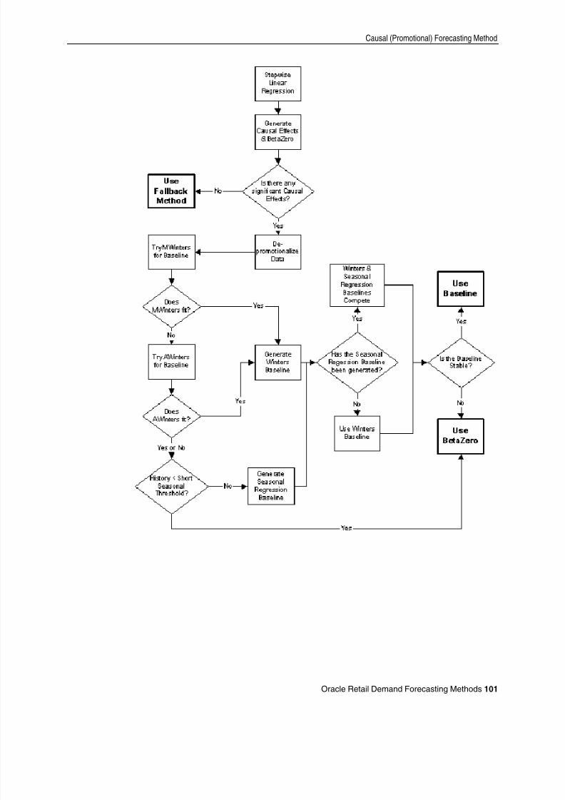
8/10/2019 RDF User Guide
http://slidepdf.com/reader/full/rdf-user-guide 111/120
Causal (Promotional) Forecasting Method
Oracle Retail Demand Forecasting Methods 101
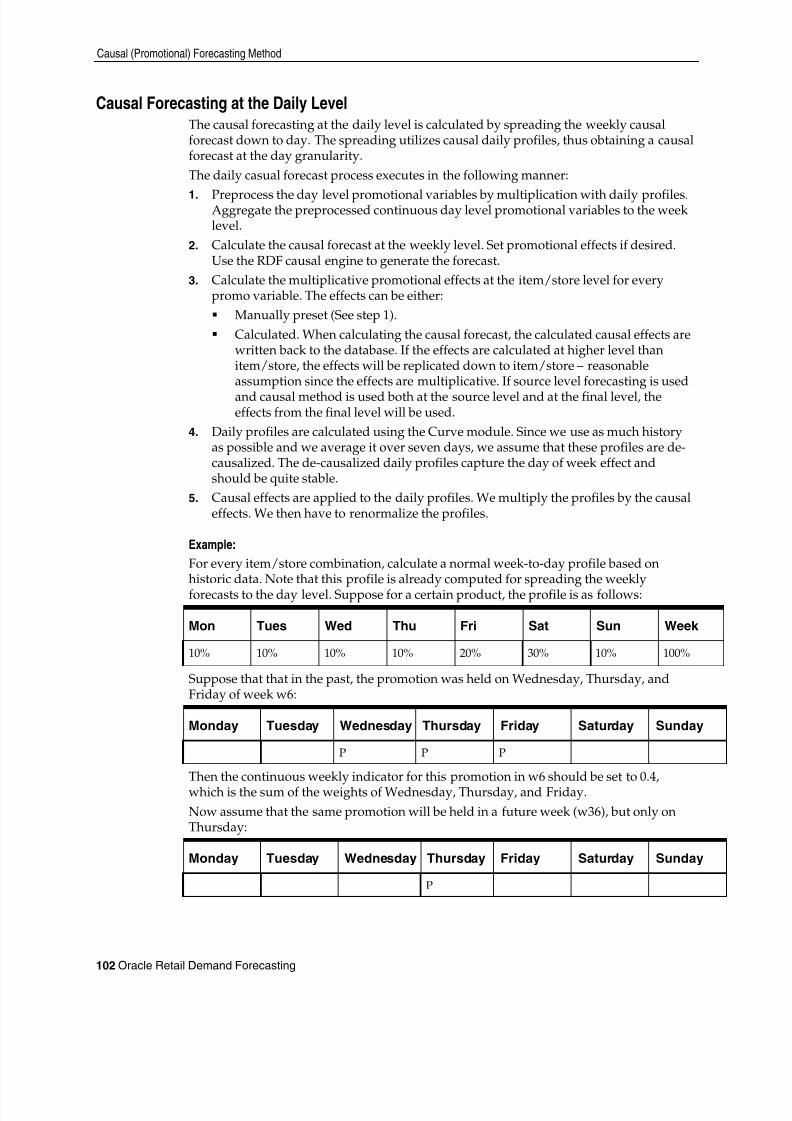
8/10/2019 RDF User Guide
http://slidepdf.com/reader/full/rdf-user-guide 112/120
Causal (Promotional) Forecasting Method
102 Oracle Retail Demand Forecasting
Causal Forecasting at the Daily LevelThe causal forecasting at the daily level is calculated by spreading the weekly causalforecast down to day. The spreading utilizes causal daily profiles, thus obtaining a causalforecast at the day granularity.The daily casual forecast process executes in the following manner:
1. Preprocess the day level promotional variables by multiplication with daily profiles.Aggregate the preprocessed continuous day level promotional variables to the weeklevel.
2. Calculate the causal forecast at the weekly level. Set promotional effects if desired.Use the RDF causal engine to generate the forecast.
3. Calculate the multiplicative promotional effects at the item/store level for everypromo variable. The effects can be either: Manually preset (See step 1). Calculated. When calculating the causal forecast, the calculated causal effects are
written back to the database. If the effects are calculated at higher level thanitem/store, the effects will be replicated down to item/store – reasonableassumption since the effects are multiplicative. If source level forecasting is usedand causal method is used both at the source level and at the final level, theeffects from the final level will be used.
4. Daily profiles are calculated using the Curve module. Since we use as much historyas possible and we average it over seven days, we assume that these profiles are de-causalized. The de-causalized daily profiles capture the day of week effect andshould be quite stable.
5. Causal effects are applied to the daily profiles. We multiply the profiles by the causaleffects. We then have to renormalize the profiles.
Example:For every item/store combination, calculate a normal week-to-day profile based onhistoric data. Note that this profile is already computed for spreading the weeklyforecasts to the day level. Suppose for a certain product, the profile is as follows:
Mon Tues Wed Thu Fri Sat Sun Week
10% 10% 10% 10% 20% 30% 10% 100%
Suppose that that in the past, the promotion was held on Wednesday, Thursday, andFriday of week w6:
Monday Tuesday Wednesday Thursday Friday Saturday Sunday
P P P
Then the continuous weekly indicator for this promotion in w6 should be set to 0.4,which is the sum of the weights of Wednesday, Thursday, and Friday.Now assume that the same promotion will be held in a future week (w36), but only onThursday:
Monday Tuesday Wednesday Thursday Friday Saturday Sunday
P
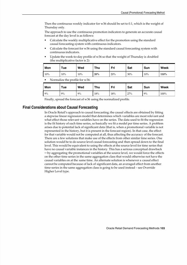
8/10/2019 RDF User Guide
http://slidepdf.com/reader/full/rdf-user-guide 113/120
Causal (Promotional) Forecasting Method
Oracle Retail Demand Forecasting Methods 103
Then the continuous weekly indicator for w36 should be set to 0.1, which is the weight ofThursday only.The approach to use the continuous promotion indicators to generate an accurate causalforecast at the day level is as follows: Calculate the weekly multiplicative effect for the promotion using the standard
causal forecasting system with continuous indicators. Calculate the forecast for w36 using the standard causal forecasting system with
continuous indicators. Update the week-to-day profile of w36 so that the weight of Thursday is doubled
(the multiplicative factor is 2):
Mon Tue Wed Thu Fri Sat Sun Week
10% 10% 10% 20% 20% 30% 10% 110%
Normalize the profile for w36:
Mon Tue Wed Thu Fri Sat Sun Week
9% 9% 9% 18% 18% 27% 9% 100%
Finally, spread the forecast of w36 using the normalized profile.
Final Considerations about Causal ForecastingIn Oracle Retail’s approach to causal forecasting; the causal effects are obtained by fittinga stepwise linear regression model that determines which variables are most relevant andwhat effect those relevant variables have on the series. The data used to fit the regressionis the fit history of each time series, so basically we fit a model per time series. A problemarises due to potential lack of significant data (that is, when a promotional variable is notrepresented in the history, but it is present in the forecast region). In that case, the effectfor that variable would not be computed at all, thus affecting the accuracy of the forecast.
There are a few solutions that make use of the effects from other similar time series. Onesolution would be to do source level causal forecasting and then spread down to the finallevel. This would be equivalent to using the effects at the source level for time series thathave no causal variable instances in the history. This has a serious conceptual drawback ─ by aggregating the promotional variables at the source level, we would force the effectson the other time series in the same aggregation class that would otherwise not have thecausal variables on at the same time. An alternate solution is whenever a causal effectcannot be computed because of lack of significant data, an averaged effect from anothertime-series in the same aggregation class is going to be used instead – see OverrideHigher Level type.

8/10/2019 RDF User Guide
http://slidepdf.com/reader/full/rdf-user-guide 114/120

8/10/2019 RDF User Guide
http://slidepdf.com/reader/full/rdf-user-guide 115/120
Glossary 105
GlossaryNote: With a few exceptions, this glossary containsdefinitions of terms specific to Oracle Retail Demand
Forecasting. For further definitions of terms and conceptsrelating to the RPAS user interface, see the RPAS Online Help or RPAS User Guide .
Additive Seasonal Method
Also referred to as Additive Winters Model, this model is similar to the MultiplicativeWinters model, but is it used when zeros are present in the data. This model adjusts theun-seasonalized values by adding the seasonal index for the forecast horizon.
Alert
A notice displayed to system users that a forecasted value is above or below user-definedlimits (an exception).
Alert Manager WindowA window that displays the alerts assigned to you. This dialog provides a list of allidentified instances in which a monitored measure’s values fall outside a set of definedlimits. You may pick an alert from this list and have RCS automatically build a workbookcontaining the measure values that triggered the alert.
AutoES Method or Automatic Exponential Smoothing Method
Oracle Retail Demand Forecasting fits the sales data to a variety of exponentialsmoothing (time series) models of forecasting, and the best model is chosen for the finalforecast. The candidate methods considered by AutoES are:
Simple ES Intermittent ES Trend ES Multiplicative Seasonal Additive Seasonal and Seasonal ES
The final selection between the models is made according to a performance criterion(Bayesian Information Criterion) that involves a tradeoff between the model’s fit over thehistoric data and its complexity.
Bayesian Method
Useful for short lifecycle forecasting and for new products with little or no historic salesdata. The Bayesian method requires a product’s known sales plan (created externally toRDF) and considers a plan’s shape (the selling profile or lifecycle) and scale (magnitudeof sales based on Actuals). The initial forecast is equal to the sales plan, but as salesinformation comes in, the model generates a forecast by merging the sales plan with thesales data. The forecast is adjusted so that the sales magnitude is a weighted average
between the original plan’s scale and the scale reflected by known history.

8/10/2019 RDF User Guide
http://slidepdf.com/reader/full/rdf-user-guide 116/120
106 Oracle Retail Demand Forecasting
Causal Method
Causal is a forecasting method used for promotional forecasting and can only be selectedif Promote is implemented. Typically, the Causal method is used at the Final Levels (thatis, item/week/week). Causal uses a Stepwise Regression sub-routine to determine thepromotional variables that are relevant to the time series and their lift effect on the series.AutoES utilizes the time series data and the future promotional calendar to generatefuture baseline forecasts. By combining the future baseline forecast and each promotion’seffect on sales (lift), a final promotional forecast is computed.
Croston’s Model of Exponential Smoothing
See Intermittent Exponential Smoothing.
Curve
An optional automated predictive solution that transforms organization-level assortmentplans into base-level weekly sales forecasts.
Exception
A forecast value that is greater than or less than a user-defined limit.
Exponential SmoothingΑ form of a weighted moving average. It weights decline in data exponentially. Mostrecent data weighted more heavily. Requires smoothing constant ( α ). Ranges from 0 to 1.Subjectively chosen.
Final Forecast Level
A low level in a hierarchy from which a forecast is generated, and at which approvalsand data exports can be performed. Often, data from forecasts at a low level isinsufficient to generate reliable forecasts without first aggregating the data to a higherlevel and then spreading the data back to the low level.
Forecast
In Oracle Retail Demand Forecasting (RDF), Forecast refers to RDF’s statisticalforecasting capabilities.
Forecast-Driven Planning
Planning that keys off of forecasts fed directly into a planning system. Connection toOracle Retail Demand Forecasting (RDF) is built directly into the business processsupported by Oracle Retail Predictive Planning through an automatic approval of aforecast that is fed directly in the planning system. This allows you to accept all or part ofSales Value forecast. Once that decision is made, the balance of business measures areplanned within Oracle Retail Predictive Planning.
Holt’s Model of Exponential Smoothing
See Trend Exponential Smoothing
Interactive Forecasting
A workbook in RDF that is used to simulate forecast by modifying parameters such asForecast Method and History Start Date
8/10/2019 RDF User Guide
http://slidepdf.com/reader/full/rdf-user-guide 117/120
Glossary 107
IntermittentES or Intermittent Exponential Smoothing
Oracle Retail Demand Forecasting fits the data to the Croston's model of exponentialsmoothing. This method should be used when the input series contains a large number ofzero data points (that is, intermittent demand data). The original time series is split into aMagnitude and Frequency series, and then the Simple ES model is applied to determinelevel of both series. The ratio of the magnitude estimate over the frequency estimate isthe forecast level reported for the original series.
Like Item or Like SKU
An item that will be used as a model to forecast a new item introduction.
Lost Sales
Periods in sales data in which there was no inventory to meet consumer demand.
Measure
Any item of data that can be represented on a grid in worksheets.
Measure Description
The description of the measure that can be viewed in a workbook. This description maycontain relationships and calculations.
Measure Function
Internal functions that can be used to simplify building calculations for a measure.
Measure Identifier
The combination of role, version, metric, and units that uniquely specifies a singlemeasure.
Metric
A measure definition with the role, version, and units omitted.
Multiplicative Seasonal
Also referred to as Multiplicative Winters Model, this model extracts seasonal indicesthat are assumed to have multiplicative effects on the un-seasonalized series.
Preprocessing
In Oracle Retail Demand Forecasting (RDF), Preprocessing refers to a module thatprocesses data before forecasts are generated to adjust for situations, such as lost salesand unusually high demand.
Profile
Spreading ratios that are used in the Curve process. Typical profiles can include storeparticipation, size distribution, and time (phase-to-week) profiles, as well as otherinformation. Profiles are generated using historical data and phase definitions, based onyour system configuration.Profile Based
Oracle Retail Demand Forecasting generates a forecast based on a seasonal profile thatcan be created in Curve or a legacy system. Profiles can also be copied from anotherprofile and adjusted. Using historic data and the profile, the data is de-seasonalized andthen fed to the Simple ES method. The Simple forecast is then re-seasonalized using theprofiles.
8/10/2019 RDF User Guide
http://slidepdf.com/reader/full/rdf-user-guide 118/120
108 Oracle Retail Demand Forecasting
Profile Spread
Used at the final level to utilize a profile (either generated externally or with Curve) todetermine the spreading ratios from the Source level forecast down to the Final level.
Promote
Promote is an optional add-on automated predictive solution that allows you toincorporate the effects of promotional and causal events, such as radio advertisementsand holiday occurrences, into your time series forecasts. The promotional forecastingprocess uses both past sales data and promotional information to forecast futuredemand.
Promotion Planning
A workbook template and simulation process used within the context of promotionalforecasting. Promotion planning involves specifying whether the event status for aparticular promotional variable is active (on) or inactive (off) for a specificproduct/location/calendar combination. When past promotional events are representedas accurately as possible, the modeling routine can more precisely detect correlation
between event occurrences and changes in sales values.
Promotional Effectiveness
A workbook template used in the context of promotional forecasting. This workbookallows you to analyze the effects of promotions on items at both the micro and the macrolevel. “What if” analysis can also be performed on the results of promotional forecasts, asyou can modify future and past promotional inputs, the system-estimated effects ofpromotions and the promotional forecasts themselves.
Promotional Forecasting
Promote’s forecasting technique (also referred to as Causal forecasting) uses promotionalfactors and events to predict future demand. Promotion events are events; such asadvertisements, holidays, competitor information, and other factors that affect thenormal selling cycle for a business.
Promotion Group
A set of products or locations that are believed to exhibit similar effects during commoncausal events. Promotion groups should be established to maximize the number of timeseries for each group (so each promotional event can be evaluated from as many differentobservations as possible) while ensuring that each time series is affected by causal eventsto the same degree.
Seasonal ES Method
A combination of several Seasonal methods. This method is generally used for knownseasonal items or forecasting for long horizons. This method applies the MultiplicativeSeasonal model unless zeros are present in the data, in which case the Additive Wintersmodel of exponential smoothing is used. If less than two years of data is available, aSeasonal Regression model is used. If there is too little data to create a seasonal forecast(in general, less than 52 weeks), the system will select from the Simple ES, Trend ES, andIntermittent ES methods.
8/10/2019 RDF User Guide
http://slidepdf.com/reader/full/rdf-user-guide 119/120
Glossary 109
Seasonal Regression
Seasonal Regression cannot be selected as a forecasting method, but it is a candidatemodel used when the Seasonal ES method is selected. This model requires a minimum of52 weeks of history to determine seasonality. Simple Linear Regression is used toestimate the future values of the series based on a past series. The independent variable isthe series history one-year or one cycle length prior to the desired forecast period, andthe dependent variable is the forecast. This model assumes that the future is a linearcombination of itself one period before plus a scalar constant.
Simple/Intermittent ES Method
A combination of the Simple ES and Intermittent ES methods. This method applies theSimple ES model unless a large number of zero data points are present. In this case, theCroston’s model is applied.
SimpleES or Simple Exponential Smoothing Method
Oracle Retail Demand Forecasting uses a simple exponential smoothing model togenerate forecasts. Simple ES ignores seasonality and trend features in the demand data,and it is the simplest model of the exponential smoothing family. This method can be
used when less than one year of historic demand data is available.Simple Moving Average
See Average Method.
Sister Store
A store that will be used as a model to forecast a new store.
Source Level Forecast
The level at which the aggregate, more robust forecast is run.
Time Series
Set of evenly spaced numerical data obtained by observing response variable at regular
time periods. This data is used to forecast based only on past values. It assumes thatfactors influencing past and present will continue influence in future.
Training Window
The number of weeks of historical sales data to use in generating a forecast.
Trend Exponential Smoothing or TrendES
Also referred to as Holt’s Model, Oracle Retail Demand Forecasting fits the data to theHolt model of exponential smoothing. The Holt model is useful when data exhibits adefinite trend. This method separates out base demand from trend, and then providesforecast point estimates by combining an estimated trend and the smoothed level at theend of the series.
WizardA set of screens that guide you through the process of creating a new workbook orperforming other actions in a solution by asking you various questions and having youselect values.
Workbook
The framework used for displaying data and user functions. Workbooks are task-specificand may contain one or more worksheets. Users define the format of their workbooks.Also see workbook template, worksheet.

8/10/2019 RDF User Guide
http://slidepdf.com/reader/full/rdf-user-guide 120/120
Workbook Template
The framework for creating a workbook. You build each new workbook from an existingworkbook template, such as Pre-Season Financial Plan or Forecasting Administration.Several workbook templates are supplied with the Oracle Retail Predictive Solutions, andare available for selection when you choose File – New to create a new workbook.
WorksheetA multidimensional spreadsheet used to display workbook-specific information.Worksheet data can also be displayed in chart format.