STA305 week 10 1

RCB - Example

• An accounting firm wants to select training program for its auditors who conduct statistical sampling as part of their job.

• Three training methods are under consideration: home study, presentations by local staff and training sessions at head office.

• 30 auditors were placed into one of 10 groups of 3 based on time since graduation.

• Within each group, one auditor was randomly allocated to each of the 3 training methods a proficiency exam was administered at the end of the training period.

• The results of the proficiency test are given in the following table:

STA305 week 10 2

STA305 week 10 3

• As we can see on average, training at the head office tends to produce the highest proficiency scores.

• The blocks appear to be quite heterogeneous with respect to proficiency.

• The sums of squares and the ANOV are…

• Test that the 3 training methods result in the same mean proficiency scores…

STA305 week 10 4

Linear Contrasts• As we have seen previously, the ANOVA will tell us only if there is

an overall difference between the treatment means.• In order to test hypotheses about the equality of specific treatment

means, we use linear contrasts.• The contrasts, the corresponding hypothesis and the test statistic are

the same as before.• Hypothesis: H0 : c1μ1 + c2μ2 + · · · + caμa = 0

Ha : c1μ1 + c2μ2 + · · · + caμa ≠ 0• Test statistic is:

• So P-value = P(F(1,(a-1)(b-1)) > Fobs)

( )( )( )( )11,1

12

2

1 ~/

−−

=

= •

∑∑= baa

i iE

a

i iiobs F

bcMS

YcF

STA305 week 10 5

Tests Concerning Block Means

• From an examination of the expected mean squares, it would seem reasonable to test :

H0: β1 = β2 = ... = βb = 0by comparing MSBl / MSE to the critical F value.

• However, when we applied randomization, we did so only within blocks.

• Some authors argue that because of the restriction on randomization that we imposed, this F test would be a test of the equality of block plus restriction effect.

Increased Precision Due to Blocking

• In designing the study, we decided to use blocks and impose a restriction on randomization.

• We did this because we believed that by controlling the nuisance factor we would decrease haphazard error.

• We might be interested in knowing how much we gained by blocking.

• The test for equality of block means is open to interpretation, and even it wasn’t, it would not help quantify any gains due to blocking.

• Several authors have proposed a measure of the relative gain in efficiency due to inclusion of the blocking factor.

• Their measure takes into account the fact that in the completely randomized (CR) design there are more degrees for freedom for estimating error variability.

STA305 week 10 6

• It is given by

• In this expression, is the experimental error variance of the completely randomized design, and is the corresponding quantity from the randomized complete block design.

• In order to estimate R, we must first estimate and .

• We can use MSE from the randomized block design to estimate .

• Further, it can be shown that an unbiased estimator of is

where MSBLis the mean square for blocks from the randomized complete block design.

STA305 week 10 7

( )( )( )( ) 2

2

1331

BL

CR

CRBL

CRBL

dfdfdfdfR

σσ

×++++

=

2CRσ

2CRσ

2CRσ

2BLσ

2BLσ

2BLσ

( ) ( )1

112

−−+−

=ab

MSabMSb EBLCRσ

Example

• Consider the example of the accounting firm that was interested in selecting the best of 3training methods.

• The study used time since graduation as a blocking variable.

• To find the efficiency of this design relative to the completely randomized design, we need the following…

STA305 week 10 8

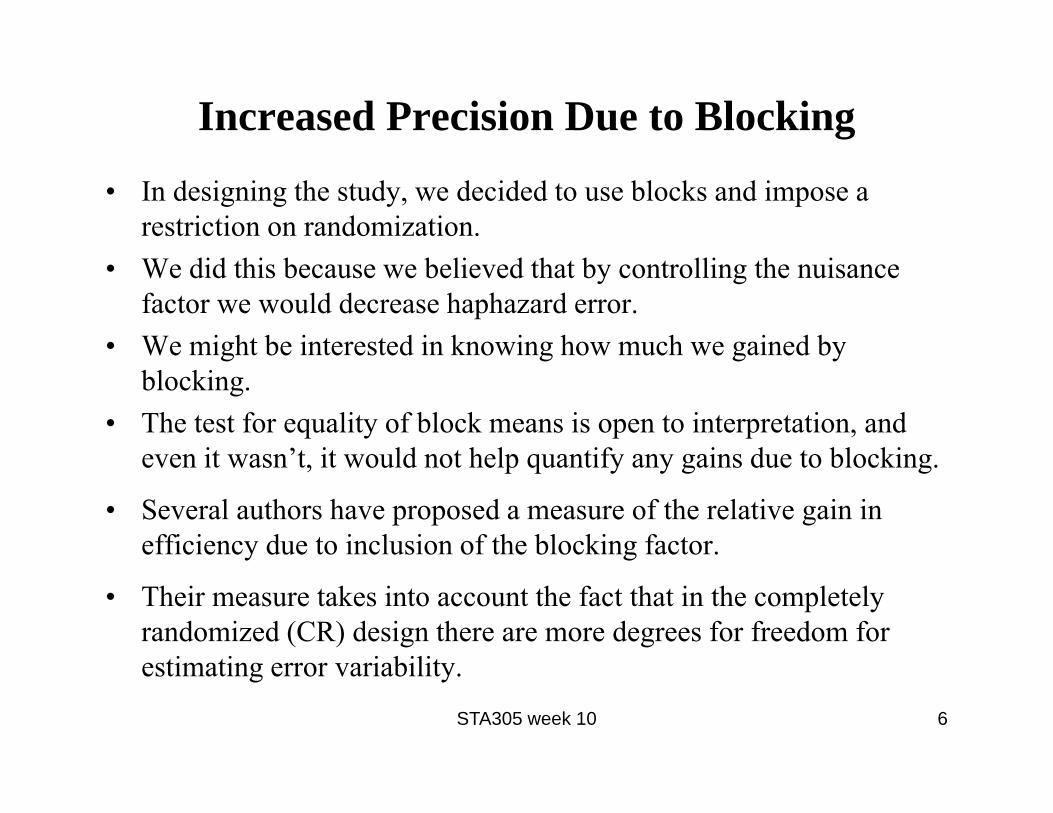
RCB ANOVA Using SAS

• The SAS procedure that we will use to conduct the analysis of variance in the randomized complete block design is GLM.

• In fact, we will use the same commands as in the two factor fixed effect model.

• As usual, start by inputting the data…

• The ANOVA for the previous example is produced as follows:

proc glm data = example ;class years program ;model score=years program ;run ;

STA305 week 10 9

Assessing Model Adequacy

• As in the case of the one factor model, we made a number of assumptions about the data that we must verify.

• Once the model has been fit, the residuals should be examined to assess the validity of the normality assumption.

• Similarly, the variance should be examined within each treatment and within each block to ensure homogeneity.

• The same tools can be used here as in the one factor case: scatterplots, box plots, and normal probability plots.

STA305 week 10 10

Replication and Interaction

• The model we used for the randomized complete block design assumes that the size and direction of the treatment effect is the same within each block.

• We would need more than 1 observation per treatment within each block to look for interaction of treatments with blocks.

• We will handle this case in the same manner as in the two-factordesign.

STA305 week 10 11

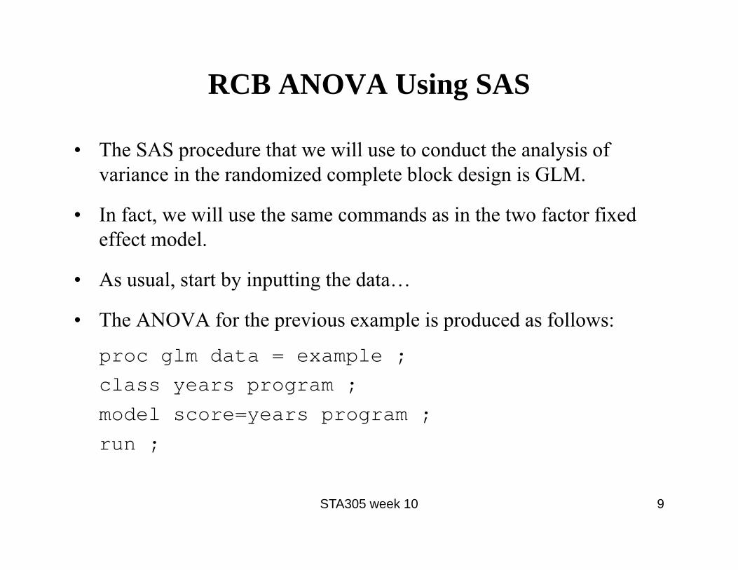
Estimating Model Parameters

• One method of estimating the model parameters involves minimizing the squared distances from the “fitted” model to the observed response values.

• That is, we need to find the values of μ, τi, and βj which minimize

• Differentiate Q with respect to each of the parameters, set resulting equations to 0, and solve for the parameter values….

STA305 week 10 12

( )∑∑= =

−−−=a

i

b

jjiijYQ

1 1

2βτμ

Exercise

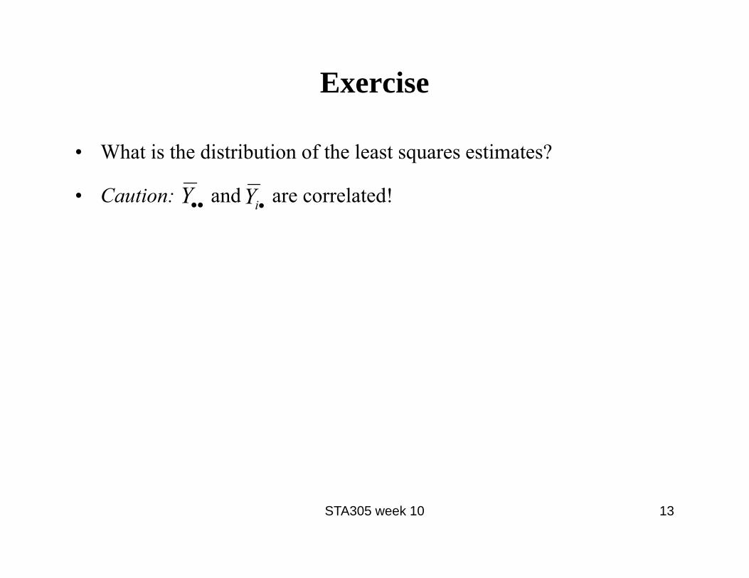
• What is the distribution of the least squares estimates?

• Caution: and are correlated!

STA305 week 10 13

••Y •iY

Latin Square Design

• Recall: the purpose of blocking was to minimize variability due to known & controllable nuisance factor.

• There may be more than one nuisance factor that is known & controllable.

• We will now examine the case where there are 2 such nuisance factors.

STA305 week 10 14

Example

• Output of 4 industrial processes to be compared.

• The processes usually only run on Mon, Wed, Fri, and Sat. We can run several processes on each day.

• Processes are affected by external conditions such as weather which vary day to day.

• The external conditions also vary by time of day.

• In studying the 4 processes, we need to ensure each process runs in each time slot on each day.

• The 4 processes form the treatments in this study, while day and time of day are 2 nuisance factors which are known & controllable.

STA305 week 10 15

• One possible way to run this study is described in the following table

• This allocation ensures that there is a balance with respect to day of the week and time of day. That is, each process is run on each day and each process is run in each time slot.

• This is an example of a Latin Square design.

• Each of the nuisance factors must have the same number of levels as the factor being studied.

STA305 week 10 16

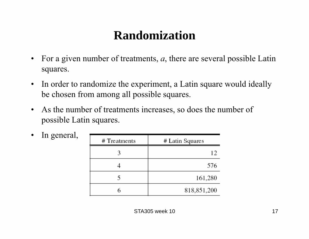
Randomization

• For a given number of treatments, a, there are several possible Latin squares.

• In order to randomize the experiment, a Latin square would ideally be chosen from among all possible squares.

• As the number of treatments increases, so does the number of possible Latin squares.

• In general,

STA305 week 10 17

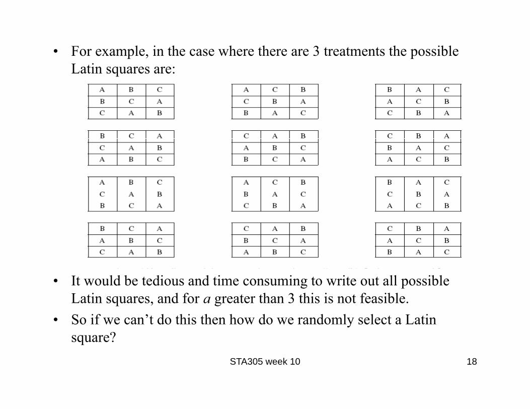
• For example, in the case where there are 3 treatments the possible Latin squares are:

• It would be tedious and time consuming to write out all possible Latin squares, and for a greater than 3 this is not feasible.

• So if we can’t do this then how do we randomly select a Latin square?

STA305 week 10 18

Standard Latin Squares• A standard Latin square is one which has both the first row and the

first column in numeric (or alphabetic) order.• For example,

• To randomize, start with the standard Latin square and randomly permute the rows and columns.

• This is still difficult when the number of treatments is large.• Cyclic squares, in which treatments always follow each other in the

same order are often used in large designs.• Disadvantages: order effect, know which treatment comes next.

STA305 week 10 19

The Model for Latin Square

• We will assume that the effect of the treatment is the same regardless of the level of the 2 nuisance factors, i.e., we assume that the factors do not interact with each other.

• The model is then….

STA305 week 10 20

Notation

• We will use the “dot” notation with 3 subscripts…

STA305 week 10 21

Sources of Variation

• Possible sources of variability in this model, include:

Differences in treatment meansDifferences in means for each row levelDifferences in means for each column levelRandom variability

• The total sum of squares can be partitioned in the usual manner:

STA305 week 10 22

Hypothesis Testing

• Although this design involves 3 factors, only one is of primary interest.

• The other 2 are nuisance factors and are included in the design to minimize experimental error.

• The hypothesis about the equality of treatment means can be tested in a manner similar to that used in the CR and randomized complete block designs.

• The hypothesis of interest is:H0: μ1 = μ2 =....= μa versus Ha: not all μi equal orH0:τ1 = τ2 = ... = τa =0 versus Ha: not all τi = 0

• To begin, construct the analysis of variance table. It is given in the next slide…

STA305 week 10 23

STA305 week 10 24

Example

• A medical researcher was interested in comparing four formulas that were fed to newborn infants.

• The outcome of interest was the weight gain (in ounces per day) after one week.

• The study was designed in such a way that each formula was to be fed to each infant for 1 week.

• Four infants participated in the study, and 4 weeks were needed to complete the study

• Although primary interest was in the difference in mean weight gain between the 4 formulas, two nuisance factors which could affect the outcome were identified.

STA305 week 10 25

• These were: (a) infants, i.e. some infants may gain weight more quickly than

others.(b) week i.e. the week determines the age of the infant, which could

affect outcome and week could also be an indicator for external conditions i.e. in week x there was a flu virus circulating which caused weight loss.

• The following table indicates Latin square that was randomly selected to determine when infants would receive formulas 1-4

STA305 week 10 26

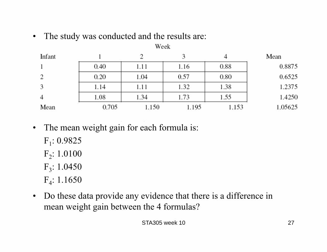
• The study was conducted and the results are:

• The mean weight gain for each formula is:F1: 0.9825F2: 1.0100F3: 1.0450F4: 1.1650

• Do these data provide any evidence that there is a difference in mean weight gain between the 4 formulas?

STA305 week 10 27

Solution

• Before proceeding to the analysis of variance, examine the sample means so we know what to expect.

• We blocked on 2 factors in the belief that there was considerable variability within blocks, and less variability between blocks.

• Does blocking on these 2 variables appear to have been worthwhile?

• One of the blocking factors was infant; there seems to be quite a bit a difference in average weight gain for the 4 infants, so perhaps this was worthwhile including in the design.

• The second blocking factor was week; the mean weight gain for weeks 2-4 do not appear to differ very much; however, the weight gain in week 1 was quite a bit less, so perhaps it was a good idea to have included this in the study design.

STA305 week 10 28

• The factor of primary interest was the type of formula that was fed to the infants.

• Although there are some differences between the formulas, these differences aren’t as pronounced as the differences between infants.

• Need to conduct the ANOVA to determine whether the differences are significant.

• Start by calculating the sums of squares…

STA305 week 10 29

Latin Squares Using SAS

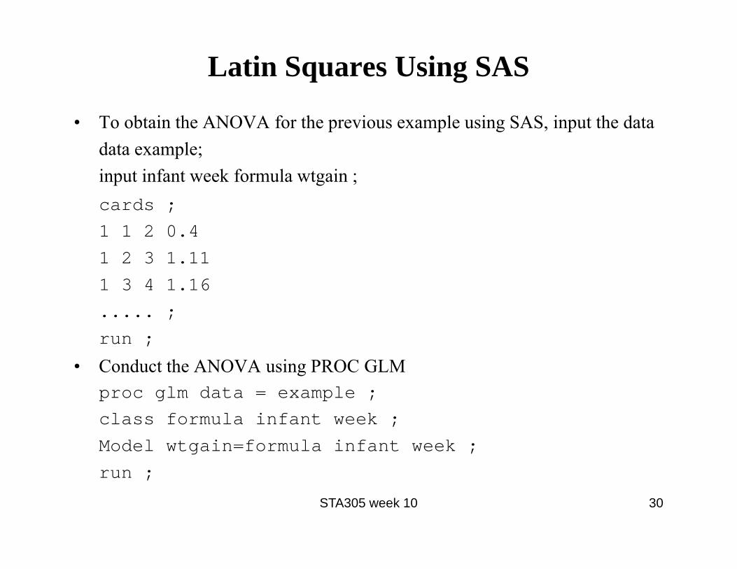
• To obtain the ANOVA for the previous example using SAS, input the datadata example;input infant week formula wtgain ;cards ;1 1 2 0.41 2 3 1.111 3 4 1.16..... ;run ;

• Conduct the ANOVA using PROC GLMproc glm data = example ;class formula infant week ;Model wtgain=formula infant week ;run ;

STA305 week 10 30

Advantages / Disadvantages of Latin Square Design

• One of the advantages of the Latin square design is that the use of 2 blocking variables can greatly reduce experimental error.

• The total number of experimental units required is relatively small, which makes this design very practical for pilot or preliminary studies.

• One of the drawbacks of using a Latin square design is that the number of levels of each nuisance factor must equal the number of treatments.

• In some cases, the complexity of the randomization can be a disadvantage.

• The degrees of freedom for estimating σ2 are relatively small, meaning that we will not have a very precise estimate.

STA305 week 10 31

Relative Efficiency

• The Latin square is a design one level more complicated that the randomized complete block design.

• It is worth asking whether the added complexity of the Latin square paid off in terms of increased precision and power.

• Consider the simpler randomized complete block design where control of the row factor is part of the design, and column effects will (hopefully) be averaged out by randomization.

STA305 week 10 32

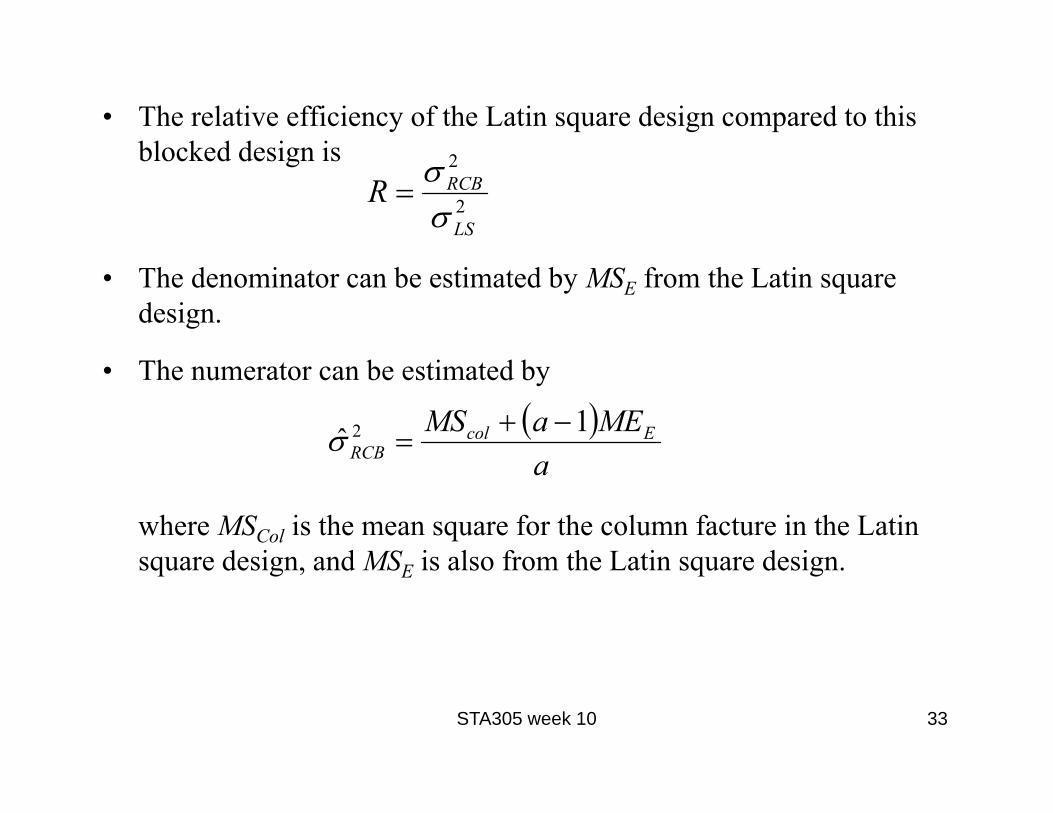
• The relative efficiency of the Latin square design compared to this blocked design is

• The denominator can be estimated by MSE from the Latin square design.

• The numerator can be estimated by

where MSCol is the mean square for the column facture in the Latin square design, and MSE is also from the Latin square design.

STA305 week 10 33

2

2

LS

RCBRσσ

=

( )a

MEaMS EcolRCB

1ˆ 2 −+=σ

Example• In the infant formula example, we might wonder whether there was

any gain in efficiency by blocking on weeks and infants, as compared to just blocking on infants.

• An estimate of the relative efficiency is obtained by first calculating the numerator

• So the relative efficiency is R = 0.0926 / 0.0521 = 1.78.

• Had we decided to use a design which blocked on infant and randomized order of formula within each infant, we would have required approximately twice the number of observations to obtain the same precision.

STA305 week 10 34

( ) 0926.04

0521.032141.01ˆ 2 =⋅+

=−+

=a

MEaMS EcolRCBσ

Replicated Latin Squares

• In general, even when the number of treatments is large, residual degrees of freedom in Latin Square remains relatively small.

• When there are only two treatments (a = 2) there are no degrees of freedom for error.

• It may be desirable to replicate the experiment in order to increase precision.

• That is, we want to increase the number of experimental units and still maintain the balance.

• To do this we must add one or more Latin squares to the experiment.

• Depending on the study, there may be more than one way to add replicates.

STA305 week 10 35

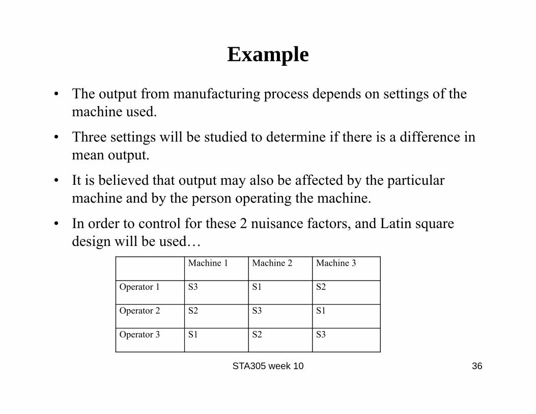
Example

• The output from manufacturing process depends on settings of the machine used.

• Three settings will be studied to determine if there is a difference in mean output.

• It is believed that output may also be affected by the particular machine and by the person operating the machine.

• In order to control for these 2 nuisance factors, and Latin square design will be used…

STA305 week 10 36

Machine 1 Machine 2 Machine 3

Operator 1 S3 S1 S2

Operator 2 S2 S3 S1

Operator 3 S1 S2 S3

• If we wish to increase size of experiment and to add more experimental units, we can do it in several ways by adding more squares.

• We can either use the same operators and machines, or if possible by including new operators and machines.

• Several options are presented…

STA305 week 10 37

Example• Retraining program to teach automobile repair skills to individuals.

• Three incentive methods are being tested for use in the retraining program.

• It is believed that age and level of formal education also have an impact on outcome of training.

• There are 18 study participants available to participate in this experiment.

• Two Latin squares with the same rows and columns were used to design the

STA305 week 10 38

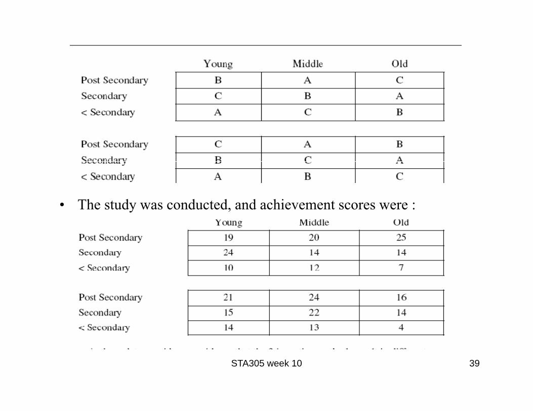
• The study was conducted, and achievement scores were :

STA305 week 10 39

Graeco-Latin Squares

• The Latin square design was used to control for 2 nuisance factors.

• When there is a 3rd nuisance factor to be included in the design of an experiment, Graeco- Latin squares are used.

• A Graeco-Latin square consists of superimposing 2 orthogonalLatin squares.

• Consider 2 Latin squares, one with Latin letters and one with Greek letters.

• The 2 squares are said to be orthogonal if each Latin letter appears exactly once with each Greek letter.

STA305 week 10 40

Example

STA305 week 10 41