Final Project – March Madness Points Scored

Raymond Romaniuk

Student #: 6047088

Brock University

MATH 4P81

Due Date: November 30, 2020

Abstract

This project intends to determine the best sampling method to estimate points scored in

March Madness College Basketball games. This research is valuable to a basketball coach

looking for an advantage in the tournament. The three methods we will use are Simple Random

Sampling Without Replacement, Stratified Random Sampling with Proportionate Allocation and

Stratified Random Sampling with Neyman Allocation. Using the three sampling methods we

compare their mean and standard deviation to the population mean and standard deviation to

check how accurate our samples are. We also find the variance and standard error of our

estimated mean and use these to compare the precision of our estimates. Ultimately it seems that

the Stratified Random Sample with Neyman Allocation is the best option in this scenario. This

information will help coaches understand how many points their team will need to be prepared to

score when competing in March Madness. March Madness provides schools the opportunity to

get their name recognized on a national scale and can positively impact schools far beyond just

the scope of basketball.

Key Words

Basketball, National Collegiate Athletic Association, March Madness, Points Scored, Random

Sampling, Simple Random Sample, Stratified Random Sample, Proportional, Neyman

Introduction

The National Basketball Association (NBA) is regarded as one of the four major sports

leagues in North America, alongside the National Football League (NFL), National Hockey

League (NHL) and Major League Baseball (MLB). Basketball is a team sport played between

two teams with five players from each team on the playing surface, known as the court, at any

given time. The objective of the game is to shoot the basketball through the opposing teams

hoop and accumulate more points than your opponent. Points can be scored in two separate

categories, field goals and free throws. A field goal is scored during live play and can be worth

either two or three points, called a two or three pointer. The amount of points a field goal is

worth is dictated by the position on the court the shooting player shot the ball from. If it was

from behind the three-point line (see Figure 1) the shot is worth three points and if it is from

inside the three-point line the shot is only worth two points. The second method of scoring is by

free throws, these are worth one point each. A free throw occurs when a player commits an

infraction, known as a foul, on the opposition and their opponent is awarded a given number of

free throws based on the severity of the foul. Free throws take place from the free throw line

with no infringement allowed by the opposition. The NBA being a significant focal point in

North American sports leads fans to gravitate not just to the NBA, but also to National Collegiate

Athletic Association Division I Basketball, NCAA Basketball or College Basketball for short,

where the majority of future NBA players come from.

Figure 1: Diagram of important basketball court locations

This project aims to explore College Basketball, specifically the NCAA Division I Men’s

Basketball Tournament, known as March Madness. The March Madness Tournament is the

culmination of each College Basketball season and brings 68 of the top teams in the country

together to form a bracketed tournament and compete for the distinction of being the best team in

Division I College Basketball. Teams gain entry to the tournament through two avenues,

automatic bids and at large bids. Of the 68 teams, 32 of them receive automatic bids into the

tournament. To receive an automatic bid a team must win their respective conference’s playoff

tournament. There are 32 conferences, so these 32 teams are the 32 conference champions. The

36 at large bids are comprised of teams who did not win their conference’s playoff tournament.

These 36 teams are chosen by the Selection Committee who selects the 36 teams they believe are

most deserving of competing in the tournament. Teams are then seeded from 1 to 68 and split

into four different regions, East, West, South and Midwest. There are 16 teams allocated to each

region and seeded from 1 to 16 within the region. The teams are then bracketed by their seed

and the opening round consists of games with the first seed playing the sixteenth seed, second

playing fifteenth and so on. Noticeably 16 teams per region does not divide the total 68 teams

evenly. An eight-team play-in round, called the First Four, is contested prior to the first round

between the four lowest ranked automatic bid teams and the four lowest ranked at large bid

teams. The lowest ranked automatic bid teams are usually seeded lower, overall, than the lowest

ranked at large bid teams, since they are representing weaker conferences. The four automatic

bid teams thus play each other for one of two available 16 seed spots, whereas the four at large

bid teams play each other for one of two available 11 seed spots. March Madness consists of six

rounds and a total of 67 games.

Figure 2: 2019 March Madness Tournament Bracket

For this project we are putting ourselves in the place of a college basketball coach of a

team hoping to lead them to the March Madness tournament. Our schools Athletic Director

believes that our team has a chance to be successful this year and wishes to sample results from

previous tournaments, so that we knows how many points we will need to be prepared to score in

order to win. The Athletic Director wishes for us to sample game results from the past two

tournaments (2018 and 2019) using three sampling methods: a simple random sample, a

stratified random sample with proportional allocation and a stratified random sample with

Neyman allocation.

About the Data

Using the Beautiful Soup package in Python, NCAA Men’s Basketball data was scraped

for the 2017-18 and 2018-19 seasons. This data came from four different sources: ESPN, Fox

Sports, the NCAA and the Pomeroy College Basketball Ratings. These four data sources

provide a plethora of variables, however for the sake of this project we will only be using points

scored and the seed of the team that scored the points. Table 1 shows a subset of the dataset.

March Madness consists of 67 games each year, four games in the “First Four” play-in

round, 15 games in each of the four regions and three games in the “Final Four”. In the dataset

each game corresponds to two observations, see Figure 3, that means that each tournament

accounts for 134 observations. Since we have data for two tournaments, we have a total of 268

observations.

Figure 3: Data Layout For A Single Tournament Game

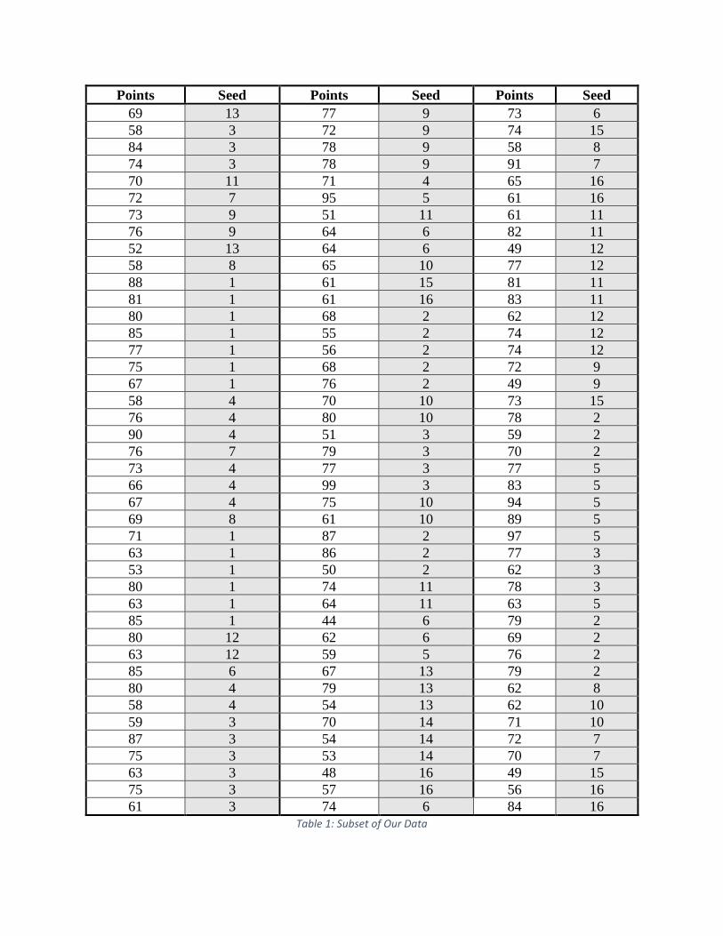
Points Seed Points Seed Points Seed

69 13 77 9 73 6

58 3 72 9 74 15

84 3 78 9 58 8

74 3 78 9 91 7

70 11 71 4 65 16

72 7 95 5 61 16

73 9 51 11 61 11

76 9 64 6 82 11

52 13 64 6 49 12

58 8 65 10 77 12

88 1 61 15 81 11

81 1 61 16 83 11

80 1 68 2 62 12

85 1 55 2 74 12

77 1 56 2 74 12

75 1 68 2 72 9

67 1 76 2 49 9

58 4 70 10 73 15

76 4 80 10 78 2

90 4 51 3 59 2

76 7 79 3 70 2

73 4 77 3 77 5

66 4 99 3 83 5

67 4 75 10 94 5

69 8 61 10 89 5

71 1 87 2 97 5

63 1 86 2 77 3

53 1 50 2 62 3

80 1 74 11 78 3

63 1 64 11 63 5

85 1 44 6 79 2

80 12 62 6 69 2

63 12 59 5 76 2

85 6 67 13 79 2

80 4 79 13 62 8

58 4 54 13 62 10

59 3 70 14 71 10

87 3 54 14 72 7

75 3 53 14 70 7

63 3 48 16 49 15

75 3 57 16 56 16

61 3 74 6 84 16

Table 1: Subset of Our Data

Population Characteristics

March Madness provides college basketball fans with an opportunity to see how teams

from different conferences fair against one another and creates interesting scenarios where the

best team from one conference could potentially be dominated by a mid level team in one of the

top conferences. Plotting points scored in a histogram the data seems to resemble a normal

distribution, looking somewhat “bell” shaped (Figure 4). Points scored has a mean of

approximately 70.3545 and standard deviation of approximately 11.9216. As we can see, in

Figure 4, there is a wide variation in points scored having such a variety of teams in the

tournament. For example, in 2018 North Carolina Central was the 272nd ranked team out of the

351 teams in the country, but since they won their conference they were able to compete in the

tournament.

Figure 4: Points Scored in 2018 and 2019 March Madness Games

Sample Factors

The Athletic Director of our school believes that the most recent tournaments will be

most representative of what our team will face if we make it to this year’s tournament. This

means that for this project our sampling frame is all 134 games played in the past two

tournaments.

Sampling Methods: Simple Random Sample Without Replacement

The first sampling method suggested by our Athletic Director is a simple random sample.

To perform a simple random sample, we must first find how many observations we need to

sample from our population of 268. We have been advised that our variance of �̅�𝑆𝑅𝑆 should not

exceed 𝑣 = 4. Now to determine the necessary sample size we solve for 𝑛 ≥ 𝑛𝑒

1+ 𝑛𝑒𝑁

, where

𝑛𝑒 = 𝑆2

𝑣. We already know that 𝑁 = 268, our population size, and by Python (attached) 𝑆2 ≈

142.1248. Solving for n, with Python, we find that the necessary size of our simple random

sample is 32.

To select our sample of 32 observations we use the method of Simple Random Sampling

Without Replacement. For our purposes placing observations that have been selected back into

the population does not make much sense, since we would like as many different observations as

possible. Thus, a Simple Random Sample Without Replacement makes more sense, in our case,

than one With Replacement. Using Python, we receive the sample in Table 2 below.

Points

49 81 64

68 62 68

46 55 52

78 61 89

71 55 61

67 56 57

73 63 89

64 59 88

68 83 44

62 71 85

63 75

Table 2: Simple Random Sample Without Replacement of Points Scored

Our Simple Random Sample has a mean of approximately 66.46875 points and standard

deviation of approximately 12.3078 points. Plotting our 32 observations of points scored in a

histogram (see Figure 5), we see that, apart from the 8 observations of 61-65 points, our

observations don’t vary much between point ranges. Having the spike at 61-65 helps since it is

in the middle, but ultimately, we have heavy tails on both sides, and this may not be the best

sample for our team to rely on.

Figure 5: Histogram of our Simple Random Sample Without Replacement

To determine whether we can continue under the assumption that our data is normally

distributed we perform a normality test. By performing the Shapiro-Wilk test in Python, we get

a p-value of 0.379. Since the p-value is greater than 0.05 we can conclude, at the 95%

confidence level, that our data follows a Normal Distribution.

Finally, using Python, we find that we have a variance of �̅�𝑆𝑅𝑆 of approximately 4.1686

and standard error of approximately 2.0417 for our Simple Random Sample Without

Replacement. Where 𝑣𝑎𝑟(�̅�𝑆𝑅𝑆) = 1−

𝑛

𝑁

𝑛 ∙ 𝑠2, with 𝑠2 =

1

𝑛−1∑ (𝑦𝑗 − �̅�)2𝑛

𝑗=1 and 𝑠𝑒(�̅�𝑆𝑅𝑆) =

√𝑣𝑎𝑟(�̅�𝑆𝑅𝑆). We will try to improve on these in our next two samples.

Sampling Methods II: Stratified Random Sample with Proportional Allocation

The second sample we will be conducting is a Stratified Random Sample with

Proportional Allocation. For comparison to our Simple Random Sample Without Replacement

we will use the n we found previously and again have a sample size of 32 observations.

For our Stratified Random Sample we will introduce a second variable from the dataset,

the seed of the opponent that we have point totals for. As mentioned above all teams in March

Madness are seeded from 1 to 16, with 1 being the best seed a team can receive and 16 being the

worst. There are four regions, so there are at least four of every seed (there are eight 11 and 16

seeds since two of each will be eliminated in the “First Four”).

We will use seed to split our data into three strata: Seeds 1-5, Seeds 6-10 and Seeds 11-

16. Table 3 shows the characteristics of these three strata. Figures 6, 7 and 8 show the

distribution of points scored for the first, second and third strata respectively. We see that they

all seem to, at least loosely, follow a Normal Distribution, however as the teams get worse the

results become more erratic and heavy tailed.

Stratum 1 (1-5) Stratum 2 (6-10) Stratum 3 (11-16)

Mean 74.1967 70.0149 64.7089

Standard Deviation 11.5820 11.3918 10.6364

Observations 122 67 79

Weight 0.4552 0.25 0.2948

Table 3: Characteristics of Our Three Strata

Figure 6: Point Distribution of Top 5 Seeded Teams

Figure 7: Point Distribution of Middle 5 Seeded Teams

Figure 8: Point Distribution of Bottom 6 Seeded Teams

To decide how many observations, of our 32, to draw from each stratum we calculate a

weight for each to determine the proportion of the total population each stratum accounts for. To

find the weight we divide 𝑁𝑖, the “Observations” in Table 2, by our total population, N, of 268.

Doing this we find weights of approximately 0.4552, 0.25 and 0.2948 for Stratum 1, 2 and 3

respectively.

Next, we multiply the weights by our total sample size of 32, to find how many

observations to draw from each stratum. Doing this we get approximately 14.5672, 8.0 and

9.43282, we will round these and choose 15 observations from Stratum 1, 8 from Stratum 2 and

9 from Stratum 3. Using Python, we obtain the sample in Table 4.

Our Stratified Random Sample with Proportional Allocation has a mean of approximately

70.5313 points and standard deviation of approximately 12.8916 points. This mean is much

closer to the population mean, of 70.3545, than our Simple Random Sample Without

Replacement, but our standard deviation is still approximately one point higher than the

population standard deviation. Now plotting our sample in a histogram, see Figure 9, it looks

much more like a normal distribution than the histogram for our Simple Random Sample.

Points

Stratum 1 (1-5) Stratum 2 (6-10) Stratum 3 (11-16)

99 83 55

62 52 57

81 58 78

80 95 43

81 86 56

80 68 64

64 61 69

68 61 74

78 73

81

71

75

83

67

54

�̅�𝟏 = 𝟕𝟒. 𝟗𝟑𝟑𝟑 �̅�𝟐 = 𝟕𝟎. 𝟓 �̅�𝟑 = 𝟔𝟑. 𝟐𝟐𝟐𝟐

Table 4: Stratified Random Sample with Proportional Allocation of Points Scored

Figure 9: Histogram of Our Stratified Random Sample with Proportional Allocation

With the help of Python, we can calculate the variance of �̅�𝑝𝑟𝑜𝑝 using the formula

𝑣𝑎𝑟(�̅�𝑝𝑟𝑜𝑝) = ∑ 𝑤𝑖2𝐻

𝑖=1 ∙ 𝑣𝑎𝑟(�̅�𝑖), where i is the stratum number (1 to 3), H is the number of

stratum, 𝑤𝑖 is the weight of the i-th stratum and 𝑣𝑎𝑟(�̅�𝑖) is the variance of the mean of the i-th

stratum calculated by 1−

𝑛𝑖𝑁𝑖

𝑛𝑖 ∙ 𝑠𝑖

2 with 𝑠𝑖2 =

1

𝑛𝑖−1∑ (𝑦𝑖𝑗 − �̅�𝑖)2𝑛𝑖

𝑗=1 . We ultimately get a variance

of �̅�𝑝𝑟𝑜𝑝 of approximately 4.1989. Taking the square root of this we get a standard error of

approximately 2.0491.

Unfortunately, both our variance and standard error of �̅�𝑝𝑟𝑜𝑝 slightly increased for our

Stratified Random Sample with Proportional Allocation opposed to our Simple Random Sample

Without Replacement. This may be due to sampling error and drawing a substandard sample or

it could be caused by other forces. We will move to our final sampling method and hopefully

find an answer.

Sampling Methods III: Stratified Random Sample with Neyman Allocation

The third, and final, sampling method we will use to try to lead our team to victory is a

Stratified Random Sample with Neyman Allocation. As with the previous two sections we will

use a sample size of 32 observations for comparisons sake. Our data remains in the same format

as with the Stratified Random Sample with Proportional Allocation, divided into three strata

based on seeding.

This time we will allocate how many observations to select from each stratum differently.

Now the number of observations drawn from each stratum will be calculated by 𝑛𝑖 = 𝑛∙𝑁𝑖∙𝑆𝑖

∑ 𝑁𝑖∙𝑆𝑖𝑘𝑖=1

,

where i is the stratum, from 1 to 3, n is our total sample size of 32, 𝑁𝑖 is the number of

observations in the i-the stratum and 𝑆𝑖 is the square root of 𝑆𝑖2 =

1

𝑁𝑖−1∑ (𝑦𝑖𝑗 − �̅�𝑖)2𝑁𝑖

𝑗=1 . Using

Python, we obtain sample sizes of 14.9612, 8.0724 and 8.9663. These exact sample sizes change

slightly from the Proportional Allocation sizes, however after rounding them they remain the

same.

Table 5 shows the Stratified Random Sample with Neyman Allocation that we obtain

using Python.

Our Stratified Random Sample with Neyman Allocation has a mean of approximately

70.09375 points and standard deviation of approximately 11.8821 points. Now both our mean

and standard deviation are very similar to the mean and standard deviation of the population.

The histogram of our sample (Figure 10) looks better than the histogram of our Simple Random

Sample, but it does not look quite as close to a Normal Distribution as our Stratified Random

Sample with Proportional Allocation.

To find the variance of �̅�𝑛𝑒𝑦 we use the formula 1

𝑛 ∑ (𝑤𝑖 ∙ 𝑠𝑖)2𝑘

𝑖=1 −1

𝑁 ∑ 𝑤𝑖 ∙ 𝑠𝑖

2𝑘𝑖=1 , where

n is our sample size of 32, N is our population size of 268, k is our three stratum, 𝑤𝑖 is the weight

of the i-th stratum (calculated in the Stratified Random Sample with Proportional Allocation

section) and 𝑠𝑖2 =

1

𝑛𝑖−1∑ (𝑦𝑖𝑗 − �̅�𝑖)

2𝑛𝑖𝑗=1 with 𝑠𝑖 being the square root of it. From this we obtain a

variance of �̅�𝑛𝑒𝑦 of 2.8024 and standard error of 1.6740. This variance and standard error

combination is lower than both the Simple Random Sample Without Replacement and Stratified

Random Sample with Proportional Allocation variances and standard errors.

Points

Stratum 1 (1-5) Stratum 2 (6-10) Stratum 3 (11-16)

64 62 62

80 67 58

65 84 61

68 54 71

75 56 55

85 76 55

70 62 72

70 79 68

80 57

62

69

77

99

102

78

�̅�𝟏 = 𝟕𝟔. 𝟐𝟔𝟔𝟕 �̅�𝟐 = 𝟔𝟕. 𝟓 �̅�𝟑 = 𝟔𝟐. 𝟏𝟏𝟏𝟏

Table 5: Stratified Random Sample with Neyman Allocation of Points Scored

Figure 10: Histogram of Our Stratified Random Sample with Neyman Allocation

Conclusion

Using Table 6 to summarize our findings, we see that our Stratified Random Sample with

Neyman Allocation seems to be best for our population. Our estimation of �̅� is the most precise

of the three methods, having the lowest variance and standard error of �̅�. It also has the closest

standard deviation to the population standard deviation while only slightly having a mean farther

from the population mean than the Stratified Random Sample with Proportional Allocation.

Characteristic Simple Random

Sample Without

Replacement

Stratified Random

Sample with

Proportional

Allocation

Stratified Random

Sample with

Neyman Allocation

Mean 66.4688 70.5313 70.0938

Standard Deviation 12.3078 12.8916 11.8821

𝑽𝒂𝒓(�̅�) 4.1686 4.1989 2.8024

𝒔𝒆(�̅�) 2.0417 2.0491 1.6740

Table 6: Summarization of the Results of Our Three Samples

It would be easy to crown the Stratified Random Sample with Neyman Allocation as the

best sampling method, however it should be noted that both our Stratified Random Samples were

using the same number of observations per strata. Our Stratified Random Sample with

Proportional Allocation had a standard deviation a whole one point higher than our Neyman

Allocation. This may have been caused by it receiving a poor sample and the Neyman

Allocation method receiving a better one.

More research will need to be performed to ultimately crown the best method, but with

the sampling we have performed I am confident, for our sake, that our Stratified Random Sample

with Neyman Allocation is the best for our purposes.

With all this sampling done I believe that we have put our team in the best position

possible to be successful in March Madness, now that we know how many points we can expect

to need to score.

References

NCAA.com, D. (2020, April 20). What is March Madness: The NCAA tournament explained.

Retrieved December 01, 2020, from https://www.ncaa.com/news/basketball-

men/bracketiq/2020-04-20/what-march-madness-ncaa-tournament-explained