Ray Tracing - cs.sjtu.edu.cnshengbin/course/cg/CS337_10_Raytracing_10.25... · Ray-tracing is the...

1 of 50

CS337 | INTRODUCTION TO COMPUTER GRAPHICS

Bin Sheng© October 25, 2016

Ray Tracing

Rendering and Techniques

Images: (Left) http://cg.alexandra.dk/?p=278, (Right) Turner Whitted ,“An improved illumination model for shaded display, ” Bell Laboratories 1980

http://cg.alexandra.dk/?p=278

http://dl.acm.org/citation.cfm?id=358882

2 of 50



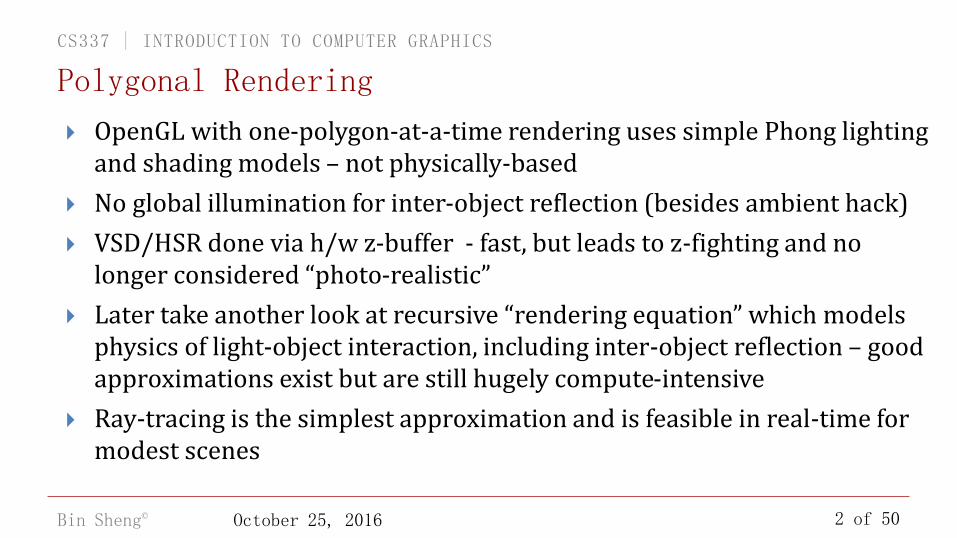
OpenGL with one-polygon-at-a-time rendering uses simple Phong lighting and shading models – not physically-based

No global illumination for inter-object reflection (besides ambient hack)

VSD/HSR done via h/w z-buffer - fast, but leads to z-fighting and no longer considered “photo-realistic”

Later take another look at recursive “rendering equation” which models physics of light-object interaction, including inter-object reflection – good approximations exist but are still hugely compute-intensive

Ray-tracing is the simplest approximation and is feasible in real-time for modest scenes

Polygonal Rendering

3 of 50



RenderingRendered with NVIDIA Iray, a photorealistic rendering solution which adds physically accurateglobal illumination on top of ray tracing using a combination of physically-based rendering techniques

iray Gallery, Image credit

http://www.nvidia.com/object/iray-image-gallery.html

http://images.nvidia.com/content/technologies/advanced-rendering/images/nvidia-iray/iray-tbn14-large.jpg

4 of 50



Introduction

What “effects” do you see?red mirror

green mirror

“soft” illumination changes

soft shadow?

No, but looks close due to complex scene and multiple light sources

Rendered in a matter of seconds with Travis Fischer’s ’09 ray tracer

5 of 50



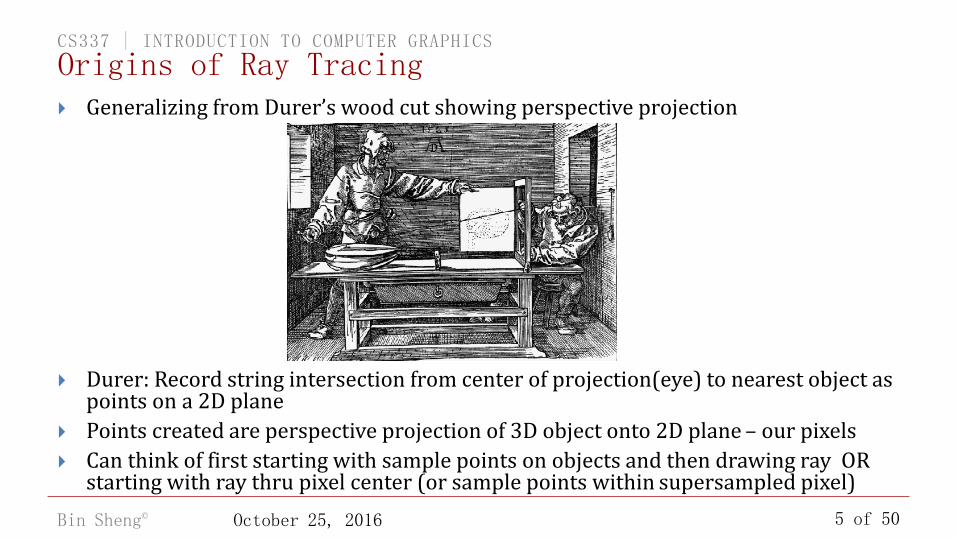
Generalizing from Durer’s wood cut showing perspective projection

Durer: Record string intersection from center of projection(eye) to nearest object as points on a 2D plane

Points created are perspective projection of 3D object onto 2D plane – our pixels

Can think of first starting with sample points on objects and then drawing ray OR starting with ray thru pixel center (or sample points within supersampled pixel)

Origins of Ray Tracing

6 of 50



A finite back-mapping of rays from camera (eye) through each sample (pixel or subpixel) to objects in scene, to avoid forward solution of having to sample from an infinite number of rays from light sources, not knowing which will be important for PoV

Each pixel represents either:

a ray intersection with an object/light in scene

no intersection

A ray traced scene is a “virtual photo” comprised of many samples on film plane

Generalizing from one ray, millions of rays are shot from eye, one through each point on film plane

What is a Raytracer?

Eye

7 of 50



Generate primary ray

shoot rays from eye through sample points on film plane

sample point is typically center of a pixel, but alternatively supersample pixels (recall supersampling from Image Processing IV)

Ray-object intersection

find first object in scene that ray intersects with (if any)

solves VSD/HSR problem – use parametric line equation for ray, so smallest t value

Calculate lighting (i.e., color)

use illumination model to determine direct contribution from light sources (light rays)

reflective objects recursively generate secondary rays (indirect contribution) that also contribute to color; RT tracing only uses specular reflection rays

Sum of contributions determines color of sample point

No diffuse reflection rays => RT is limited approximation to global illumination

Ray Tracing Fundamentals

Eye

8 of 50



How is ray tracing different from polygon scan conversion? Shapes and Sceneviewboth use scan conversion to render objects in a scene and have same pseudocode:

for each object in scene:

for each triangle in object:

pass vertex geometry, camera matrices, and

lights to the shader program,

which renders each triangle (using z-buffer)

into framebuffer; use simple or complex

illumination model

Ray Tracing vs. Triangle Scan Conversion (1/2)

(triangle rendered to screen)

9 of 50



Ray tracing uses the following pseudocode:for each sample in film plane:

determine closest object in scene hit by

a ray going through that sample from eye point

set color based on calculation of simple/complex

illumination model for intersected object

Note the distinction: polygonal scan conversion iterates over all VERTICES whereas ray tracing iterates over 2D (sub)PIXELS and calculates intersections in a 3D scene

For polygonal scan conversion must mesh curved objects while with ray tracing we can use an implicit equation directly (if it can be determined) – see Slide 14

Ray Tracing vs. Triangle Scan Conversion (2/2)

E

(ray intersection rendered to screen)

10 of 50



Ray Origin

Let’s look at geometry of the problem in normalized world space with canonical perspective frustum (i.e., do not apply perspective transformation)

Start a ray from “eye point”: P

Shoot ray in some direction d from P toward a point in film plane (a rectangle in the u-vplane in the camera’s uvw space) whose color we want to know

Points along ray have form P + td where

P is ray’s base point: camera’s eye

d is unit vector direction of ray

t is a non-negative real number

“Eye point” is center of projection in perspective view volume (view frustum)

Don’t use de-perspectivizing (unhinging) step in order to avoid dealing with inverse of non-affine perspective transformation later on – stay tuned

Generate Primary Ray (1/4)

w

11 of 50



Ray Direction

Start with 2D screen-space sample point ((sub)pixel)

To create a ray from eye point through film plane, 2D screen-space point must be converted into a 3D point on film plane

Note that ray generated will be intersecting objects in normalized world space coordinate system BEFORE the perspective transformation

Any plane orthogonal to look vector is a convenient film plane (plane z = k in canonical frustum)

Choose a film plane and then create a function that maps screen space points onto it

what’s a good plane to use? Try the far clipping plane (z = - 1)

to convert, scale integer screen-space coordinates into floats between -1 and 1 for x and y, z = -1


canonical frustum in normalized world coordinatesAny plane z = k, -1<= k < 0 can be the film plane

normalized

12 of 50



Ray Direction (continued)

Once have a 3D point on the film plane, need to transform to pre-normalization world space where objects are

make a direction vector from eye point P (at center of projection) to 3D point on film plane

need this vector to be in world-space in order to intersect with original object in pre-normalization world space

because illumination model prefers intersection point to be in world-space (less work than normalizing lights)

Normalizing transformation maps world-space points to points in the canonical view volume

translate to the origin; orient so Look points down –Z, Up along Y; scale x and y to adjust viewing angles to 45˚, scale z: [-1, 0]; x, y: [-1, 1]

How do we transform a point from the canonical view volume back to untransformed world space?

apply the inverse of the normalizing transformation: Viewing Transformation

Note: not same as viewing transform you use in OpenGL (e.g., ModelView matrix)


z=-1

13 of 50



Summary

Start the ray at center of projection (“eye point”)

Map 2D integer screen-space point onto 3D film plane in normalized frustum

scale x, y to fit between -1 and 1

set z to -1 so points lie on the far clip plane

Transform 3D film plane point (mapped pixel) to an untransformed world-space point

need to undo normalizing transformation (i.e., viewing transformation)

Construct the direction vector

a point minus a point is a vector

direction = (world-space point (mapped pixel)) – (eye point (in untransformed world space))


14 of 50



Implicit objects

If an object is defined implicitly by a function f where f(Q) = IFF Q is a point on the surface of the object, then ray-object intersections are relatively easy to compute many objects can be defined implicitly implicit functions provide potentially infinite resolution tessellating these objects is more difficult than using the implicit functions directly

For example, a circle of radius R is an implicit object in a plane, with equation:f(x,y) = x2 + y2 – R2

point (x,y) is on the circle when f(x,y) =

An infinite plane is defined by the function:f(x,y,z) = Ax + By + Cz + D

A sphere of radius R in 3-space:f(x,y,z) = x2 + y2 + z2 – R2

Ray-Object Intersection (1/5)

15 of 50



Implicit objects (continued) At what points (if any) does the ray intersect an object? Points on a ray have form P + td where t is any non-negative real number A surface point Q lying on an object has the property that f(Q) = Combining, we want to know “For which values of t is f(P + td) = ?”

We are solving a system of simultaneous equations in x, y (in 2D) or x, y, z (in 3D)


16 of 50



2D ray-circle intersection example Consider the eye-point P = (-3, 1), the direction vector d = (.8, -.6) and the unit

circle: f(x,y) = x2 + y2 – R2

A typical point of the ray is: Q = P + td = (-3,1) + t(.8,-.6) = (-3 + .8t, 1 - .6t)

Plugging this into the equation of the circle: f(Q) = f(-3 + .8t, 1 - .6t) = (-3+.8t)2 + (1-.6t)2 - 1

Expanding, we get: 9 – 4.8t + .64t2 + 1 – 1.2t + .36t2 - 1

Setting this equal to zero, we get: t2 – 6t + 9 = 0

An Explicit Example (1/3)

17 of 50



2D ray-circle intersection example (cont)

Using the quadratic formula:

We get:

Because we have a root of multiplicity 2, ray intersects circle at only one point (i.e., it’s tangent to the circle)

Use discriminant D = 𝑏2 − 4𝑎𝑐 to quickly determine if true intersection:

if 𝐷 < 0, imaginary roots; no intersection

if 𝐷 = 0, double root; ray is tangent

if 𝐷 > 0, two real roots; ray intersects circle at two points

Smallest non-negative real t represents the intersection nearest to eye-point


a

acbbroots

2

42

3 ,3 ,2

36366

tt

18 of 50



2D ray-circle intersection example (continued)

Generalizing: we can take an arbitrary implicit surface with equation f(Q) = 0,

a ray P + td, and plug the latter into the former:

f (P + td) = 0

The result, after some algebra, is an equation with t as unknown

We then solve for t, analytically or numerically


w

19 of 50



Implicit objects (continued) – multiple conditions For cylindrical objects, the implicit equation

𝑓(𝑥, 𝑦, 𝑧) = 𝑥2 + 𝑧2 – 1 = 0

in 3-space defines an infinite cylinder of unit radius running along the y-axis

Usually, it’s more useful to work with finite objects

e.g. a unit cylinder truncated with the limits:

cylinder body: 𝑥2 + 𝑧2 – 1 = 0,−1 ≤ 𝑦 ≤ 1

But how do we define cylinder “caps” as implicit equations?

The caps are the insides of the cylinder at the cylinder’s y extrema (or rather, a circle)

cylinder caps top: 𝑥2 + 𝑧2 – 1 ≤ 0, 𝑦 = 1

bottom: 𝑥2 + 𝑧2 – 1 ≤ 0, 𝑦 = −1


20 of 50



Implicit objects (continued) – cylinder pseudocodeSolve in a case-by-case approach

Ray_inter_finite_cylinder(P,d):t1,t2 = ray_inter_infinite_cylinder(P,d) // Check for intersection with infinite cylindercompute P + t1*d, P + t2*dif y > 1 or y < -1 for t1 or t2: toss it // If intersection, is it between cylinder caps?

t3 = ray_inter_plane(plane y = 1) // Check for an intersection with the top capCompute P + t3*dif x2 + z2 > 1: toss out t3 // If it intersects, is it within cap circle?

t4 = ray_inter_plane(plane y = -1) // Check intersection with bottom capCompute P + t4*dif x2 + z2 > 1: toss out t4 // If it intersects, is it within cap circle?

Of all the remaining t’s (t1 – t4), select the smallest non-negative one.If none remain, ray does not intersect cylinder


21 of 50



Implicit surface strategy summary Substitute ray (P + td) into implicit surface equations and solve for t

smallest non-negative t-value is from the closest surface you see from eye point

For complicated objects (not defined by a single equation), write out a set of equalities and inequalities and then code individual surfaces as cases…

Latter approach can be generalized cleverly to handle all sorts of complex combinations of objects constructive Solid Geometry (CSG), where objects are stored as a hierarchy of primitives and 3-D

set operations (union, intersection, difference) – don’t have to evaluate the CSG to raytrace!

“blobby objects”, which are implicit surfaces defined by sums of implicit equations (F(x,y,z)=0)


CSG!

Cool Blob!

22 of 50



To compute using illumination model, objects easiest to intersect in world space since normalizing lights with geometry is too hard and normals need to be handled. Thus need an analytical description of each object in world space

Example: unit sphere translated to (3, 4, 5) after it was scaled by 2 in the x-direction has equation

Can take ray P+td and plug it into the equation, solving for t

f (P + td ) = 0

But intersecting with an object arbitrarily transformed by modeling transforms is difficult intersecting with an untransformed shape in object’s original object coordinate system is much easier

can take advantage of transformations to change intersection problem from world space (arbitrarily transformed shape) to object space (untransformed shape)

World Space Intersection

222

2

25.0)5()4(

2

)3() , ,(

zy

xzyxf

23 of 50



To get t, transform ray into object space and solve for intersection there

Let the world-space intersection point be defined as MQ, where Q is a point in object space:

Let .

If is the equation of the untransformed object, we just have to solve

note: is probably not a unit vector the parameter t along this vector and its world space counterpart always have the same value. normalizing would alter this relationship. Do NOT normalize

Object Space Intersection

MQ

dtP

0),,( zyxf

Q

0),,(~

zyxf

24 of 50



To compute a world-space intersection, we have to transform the implicit equation of a canonical object defined in object space - often difficult

To compute intersections in object space, we only need to apply a matrix (M –1) to P and d -much simpler, but does M –1 always exist?

M was composed from two parts: the cumulative modeling transformation that positions the object in world-space, and the camera’s normalizing transformation (not including the perspective transformation!)

modeling transformations are comprised of translations, rotations, and scales (all invertible)

normalizing transformation consists of translations, rotations and scales (also invertible); but the perspective transformation (which includes the homogenization divide) is not invertible! (This is why we used canonical frustum directly rather than de-perspectivizing/unhinging it)

When you’re done, you get a t-value

This t can be used in two ways:

- 𝑷 + 𝑡𝒅 is the world-space location of the intersection between ray and transformed object

- ෩𝑷 + 𝑡෩𝒅 is the corresponding point on untransformed object (in object space)

World Space vs. Object Space

25 of 50



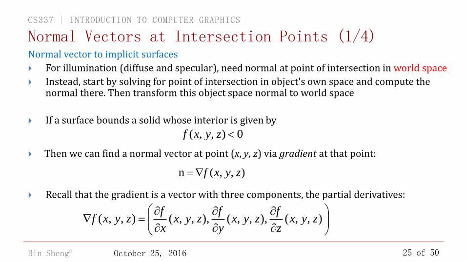
Normal vector to implicit surfaces

For illumination (diffuse and specular), need normal at point of intersection in world space

Instead, start by solving for point of intersection in object's own space and compute the normal there. Then transform this object space normal to world space

If a surface bounds a solid whose interior is given by

Then we can find a normal vector at point (x, y, z) via gradient at that point:

Recall that the gradient is a vector with three components, the partial derivatives:

Normal Vectors at Intersection Points (1/4)

0) , ,( zyxf

) , ,(n zyxf

) , ,( ), , ,( ), , ,() , ,( zyx

z

fzyx

y

fzyx

x

fzyxf

26 of 50



For the sphere, the equation is:

f (x,y,z) = x2 + y2 + z2 – 1

Partial derivatives are

So gradient is

Remember to normalize n before using in dot products!

In some degenerate cases, gradient may be zero and this method fails…nearby gradient is cheap hack


zzyxz

f

yzyxy

f

xzyxx

f

2) , ,(

2) , ,(

2) , ,(

)2,2,2(),,( zyxzyxf n

27 of 50



Transforming back to world space

We now have an object-space normal vector

We need a world-space normal vector for the illumination equation

To transform an object to world coordinates, we just multiplied its vertices by M, the object’s CTM

Can we do the same for the normal vector?

answer: NO

Example: say M scales in x by .5 and y by 2


objectworld Mnn

nobject

Mnobject Wrong!Normal must be perpendicular

28 of 50



Why doesn’t multiplying normal by M work?

For translation and rotation, which are rigid body transformations, it actually does work fine

Scaling, however, distorts normal in exactly opposite sense of scale applied to surface

scaling y by a factor of 2 causes the normal to scale by .5:

We’ll see this algebraically in the next slides


𝒏 = 1,−1

2𝒏 = 1,−

1

4

29 of 50



Object-space to world-space

As an example, let’s look at polygonal case

Let’s compute relationship between object-space normal nobj to polygon H and world-space normal nworld to transformed version of H, called MH

For any vector v in world space that lies in the polygon (e.g., one of its edge vectors), normal is perpendicular to v:

But vworld is just a transformed version of some vector in object space, vobj. So we could write:

Recall that since vectors have no position, they are unaffected by translations (thus they have w = 0)

so to make things easier, we only need to consider:

M3 = upper left 3 x 3 of M

nworld M3 vobj = 0

Transforming Normals (1/4)

0 worldworld vn

0 objworld Mvn

(rotation/scale component)

30 of 50



Object-space to world-space (continued)

So we want a vector nworld such that for any vobj in the plane of the polygon:

We will show on next slide that this equation can be rewritten as:

We also already have:

Therefore:

Left-multiplying by (M3t)-1,


0vn 3 objworld M

03 objworld

tM vn

0 objobj vn

objworld

tM nn 3

obj

t

world M nn-1

3

31 of 50



Object-space to world-space (continued) So how did we rewrite this:

As this:

Recall that if we think of vector as n x 1 matrices,

then switching notation:

Rewriting our original formula, yielding:

Writing M = M t t, we get:

Recalling that (AB)t = BtAt, we can write:

Switching back to dot product notation, our result:


a b = at b

(M3t nworld ) vobj = 0

nworld M3vobj = 0

ntworld M3vobj = 0

ntworld M3

tt vobj = 0

(M3t nworld )t vobj = 0

(M3t nworld ) vobj = 0

32 of 50



Applying inverse-transpose of M to normals

So we ended up with:

“Invert” and “transpose” can be swapped, to get our final form:

Why do we do this? It’s easier! instead of inverting composite matrix, accumulate composite of inverses which are easy to take for

each individual transformation

A hand-waving interpretation of (M3-1)t

M3 is composition of rotations and scales, R and S (why no translates?). Therefore

so we’re applying transformed (inverted, transposed) versions of each individual matrix in original order

for rotation matrix, transformed version equal to original rotation, i.e., normal rotates with object

(R-1)t = R; inverse reverses rotation, and transpose reverses it back

for scale matrix, inverse inverts scale, while transpose does nothing:

(S(x,y,z)-1)t = S(x,y,z)-1=S(1/x,1/y,1/z)


obj

t

world M nn 1

3 )(

obj

t

world M nn )(1

3

...))()(()(...)...)(( 11111 tttt SRRSRS

33 of 50



Simple, non-recursive raytracerP = eyePt

for each sample of image:

Compute d

for each object:

Intersect ray P+td with object

Select object with smallest non-negative t-value (visible object)

For this object, find object space intersection point

Compute normal at that point

Transform normal to world space

Use world space normal for lighting computations

Summary – putting it all together

34 of 50



Each light in the scene contributes to the color and intensity of a surface element…

If and only if light source reaches the object! could be occluded/obstructed by other objects in scene

could be self-occluding

Construct a ray from the surface intersection to each light

Check if light is first object intersected if first object intersected is the light, count light’s full contribution

if first object intersected is not the light, do not count (ignore) light’s contribution

this method generates hard shadows; soft shadows are harder to compute (must sample)

What about transparent or specular (reflective) objects? Such lighting contributions are the beginning of global illumination => need recursive ray tracing

Shadows

objectIntensityλ = ambient + attenuation ∙ lightIntensityλ ∙ [diffuse + specular]ΣnumLights

light = 1

35 of 50



Recursive Ray Tracing Example

Ray traced image with recursive ray tracing: transparency and refractions

Whitted 1980

36 of 50



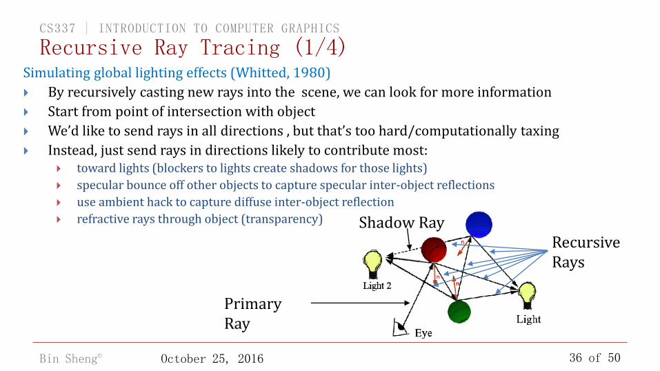
Simulating global lighting effects (Whitted, 1980)

By recursively casting new rays into the scene, we can look for more information

Start from point of intersection with object

We’d like to send rays in all directions , but that’s too hard/computationally taxing

Instead, just send rays in directions likely to contribute most: toward lights (blockers to lights create shadows for those lights)

specular bounce off other objects to capture specular inter-object reflections

use ambient hack to capture diffuse inter-object reflection

refractive rays through object (transparency)

Recursive Ray Tracing (1/4)

Shadow Ray

Primary Ray

Recursive Rays

37 of 50



Trace “secondary” rays at intersections: light: trace a ray to each light source. If light source is blocked by an opaque object, it

does not contribute to lighting

specular reflection: trace reflection ray (i.e., about normal vector at surface intersection)

refractive transmission/transparency: trace refraction ray (following Snell’s law)

recursively spawn new light, reflection, and refraction rays at each intersection until contribution negligible or some max recursion depth is reached

Limitations recursive inter-object reflection is strictly specular

diffuse inter-object reflection is handled by other techniques

Oldies-but-goodies Ray Tracing: A Silent Movie Quest: A Long Ray’s Journey into Light


https://www.youtube.com/watch?v=sg8YwRNA5j8

http://www.youtube.com/watch?v=b_UqzLBFz4Y

38 of 50



Your new lighting equation (Phong lighting + specular reflection + transmission):

I is the total color at a given point (lighting + specular reflection + transmission, λ subscript for each r,g,b) Its presence in the transmitted and reflected terms implies recursion

L is the light intensity; LP is the intensity of a point light source k is the attenuation coefficient for the object material (ambient, diffuse, specular, etc.) O is the object color fatt is the attenuation function for distance n is the normal vector at the object surface l is the vector to the light r is the reflected light vector v is the vector from the eye point (view vector) n is the specular exponent note: intensity from recursive rays calculated with the same lighting equation at the intersection point light sources contribute specular and diffuse lighting

Note: single rays of light do not attenuate with distance; purpose of fatt is to simulate diminishing intensity per unit area as function of distance for point lights (typically an inverse quadratic polynomial)


raysrecursive

ttt

reflected

rsslights

specular

n

ss

diffuse

ddpatt

ambient

aaa IOkIOkvrOklnOkLfOkLI ])()([

transmitted

39 of 50



indirect illumination

Light-ray treesRecursive Ray Tracing (4/4)

per ray:

40 of 50



Non-refractive transparency

For a partially transparent polygon

Transparent Surfaces (1/2)

Iλ2

Iλ1

polygon 1

polygon 2

2polygon for calculatedintensity

1polygon for calculatedintensity

nt transpare 1 opaque; 0

1polygon of ncetransmitta

)1(

2

1

1

2111

I

I

k

IkIkI

t

tt

41 of 50



Refractive transparency

We model the way light bends at interfaces with Snell’s Law

Transparent Surfaces (2/2)

2 medium of refraction ofindex

1 medium of refraction ofindex

sinsin

r

i

r

iir

Unrefracted(geometrical)line of sight

Medium 1

𝜃𝑖 Line of sight

Medium 2

𝜃𝑟

Refracted(optical)line of sight

Transparentobject

42 of 50



Sampling

In both the examples and in your assignments we sample once per pixel. This generates images similar to this:

We have a clear case of the jaggies

Can we do better?

Choosing Samples (1/2)

43 of 50



In the simplest case, sample points are chosen at pixel centers

For better results, supersamples can be chosen (called supersampling) e.g., at corners of pixel as well as at center

Even better techniques do adaptive sampling: increase sample density in areas of rapid change (in geometry or lighting)

With stochastic sampling, samples are taken probabilistically (recall Image Processing IV slides) Actually converges on “correct” answer faster than regularly spaced sampling

For fast results, we can subsample: fewer samples than pixels take as many samples as time permits

beam tracing: track a bundle of neighboring rays together

How do we convert samples to pixels? Filter to get weighted average of all the samples per pixel!

Choosing Samples (2/2)

Instead of sampling one point, sample within a region to create a better approximation

vs.

44 of 50



Supersampling example

With Supersampling Without Supersamping

45 of 50



Raytracer produces visible samples from model samples convolved with filter to form pixel image

Additional pre-processing pre-process database to speed up per-sample calculations

For example: organize by spatial partitioning via bins and/or bounding boxes (k-d trees, octrees, etc. - upcoming)

Ray Tracing Pipeline

Scene graph-Traverse model-Accumulate CMTM-Spatially organize objects

Object database suitable for ray-

tracingPreprocessing step

Generate rayloop over objects

intersect each with raykeep track of smallest t

Light the sample

Generate secondary rays

for each desired sample:(some (u,v) on film plane)

closest point

All samples FilterPixels of

final image

46 of 50



Traditionally, ray tracing was computationally impossible to do in real-time “embarrassing” parallelism due to independence of each

ray, so one CPU or core/pixel

hard to make hardware optimized for ray tracing:

large amount of floating point calculations complex control flow structure complex memory access for scene data

One solution: software-based, highly optimized raytracer using cluster with multiple CPUs Prior to ubiquitous GPU-based methods, ray tracing on CPU

clusters to take advantage of parallelism

hard to have widespread adoption because of size and cost

Can speed up with more cores per CPU

Large CPU render still dominant for non-real time CGI for movies and animations

Weta Digital (Planet of the Apes), ILM (Jurassic World), etc.

Real-time Ray Tracing (1/2)

OpenRT rendering of five maple trees and 28,000 sunflowers (35,000 triangles) on 48 CPUs

47 of 50



Modern solution: Use GPUs to speed up ray tracing

NVIDIA Kepler architecture capable of real time ray tracing

Demo at GTC 2012: http://youtu.be/h5mRRElXy-w?t=2m5s

Real-time Ray Tracing (2/2)

Scene ray traced in real time using NVIDIA Kepler

http://youtu.be/h5mRRElXy-w?t=2m5s

48 of 50



NVIDIA Optix framework built on top of CUDA CUDA is a parallel computing platform for nVidia GPUs

Allows C/C++ and Fortran code to be compiled and run on nVidia GPUs

Optix is a programmable ray tracing frameworkthat allows developers to quickly build ray tracingapplications

You can run the demos and download the SDKs yourself http://developer.nvidia.com/optix

http://developer.nvidia.com/cuda

GPU Ray Tracing

2015 NVIDIA Iray Demo

http://developer.nvidia.com/optix

http://developer.nvidia.com/cuda

49 of 50



GLSL shaders (like the ones you’ve been writing in lab) can be used to implement a ray tracer

OpenCL is similar to CUDA and can be used to run general purpose programs on a GPU, including a ray tracer http://www.khronos.org/opencl/

Weta Digital (Iron Man, Fantastic Four, Hunger Games) moving to GPU clusters for better efficiency

GPU Ray Tracing

http://www.khronos.org/opencl/

50 of 50



Free Advanced Raytracer Full-featured raytracer available online:

povray.org

Obligatory pretty pictures (see hof.povray.org):

POV-Ray: Pretty Pictures

Image credits can be found on hof.povray.org

http://www.povray.org/

http://hof.povray.org/

http://hof.povray.org/

Ray Tracing - cs.sjtu.edu.cnshengbin/course/cg/CS337_10_Raytracing_10.25... · Ray-tracing is the...

Documents

Transcript of Ray Tracing - cs.sjtu.edu.cnshengbin/course/cg/CS337_10_Raytracing_10.25... · Ray-tracing is the...