RAVEN: Towards Zero-Configuration LinkDiscovery

Axel-Cyrille Ngonga Ngomo, Jens Lehmann, Soren Auer, Konrad Hoffner

Department of Computer Science, University of LeipzigJohannisgasse 26, 04103 Leipzig, Germany

{ngonga|lehmann|auer}@informatik.uni-leipzig.de,konrad.hoeffner@uni-leipzig.de

WWW home page: http://aksw.org

Abstract. With the growth of the Linked Data Web, time-efficient ap-proaches for computing links between data sources have become indis-pensable. Yet, in many cases, determining the right specification for alink discovery problem is a tedious task that must still be carried outmanually. In this article we present RAVEN, an approach for the semi-automatic determination of link specifications. Our approach is basedon the combination of stable solutions of matching problems and activelearning leveraging the time-efficient link discovery framework LIMES.RAVEN is designed to require a small number of interactions with theuser in order to generate classifiers of high accuracy. We focus withRAVEN on the computation and configuration of Boolean and weightedclassifiers, which we evaluate in three experiments against link specifi-cations created manually. Our evaluation shows that we can computelinking configurations that achieve more than 90% F-score by asking theuser to verify at most twelve potential links.

Keywords: Linked Data, Link Discovery, Algorithms, Constraints

1 Introduction

The rationale of the Linked Data paradigm is to facilitate the transition from thedocument-oriented to the Semantic Web by extending the current Web with acommons of interlinked data sources [6]. Two key challenges arise when trying todiscover links between data sources: the computational complexity of the match-ing task per se and the selection of an appropriate configuration for maximizingprecision and recall.

The first challenge lies in the a-priori complexity of a matching task beingproportional to the product of the number of instances in the source and targetdata source, an unpractical proposition as soon as the source and target knowl-edge bases become large. With the LIMES framework1 [30, 29], we addressedthis challenge by providing a lossless approach for time-efficient link discoverythat is significantly faster than the state-of-the-art.

1 http://limes.sf.net

The second challenge of the link discovery process lies in the specification ofan appropriate configuration for the tool of choice. Such a specification usuallyconsists of (1) a set of restrictions on the source and target knowledge base, (2)a list of properties of the source and target knowledge base to use for similaritydetection, (3) a combination of suitable similarity measures (e.g., Levenshtein[24]) and (4) similarity thresholds. Until now, such link discovery specificationsare usually defined manually, in most cases via a time-consuming trial-and-error approach. Yet, the choice of a suitable configuration decides upon whethersatisfactory links can be discovered. Specifying complex link configurations isa tedious process, as the user does not necessary know which combinations ofproperties lead to an accurate linking configuration. The difficulty of devisingsuitable link discovery specifications is amplified on the Web of Data by thesheer size of the knowledge bases (which often contain millions of instances) andtheir heterogeneity (i.e., by the complexity of the underlying ontologies, whichcan contain thousands of different types of instances and properties) [6].

In this paper, we present the RApid actiVE liNking (RAVEN) approach.To the best of our knowledge, RAVEN is the first approach to apply activelearning techniques for the semi-automatic generation of specifications for linkdiscovery. Our approach is based on a combination of stable matching problems(as known from machine learning) and a novel active learning algorithm derivedfrom perceptron learning. RAVEN allows to determine:

– A sorted matching of classes to interlink ; this matching represents the setof restrictions on the source and target knowledge bases.

– A stable matching of properties based on the selected restrictions that spec-ifies the similarity space within which the linking is to be carried out.

– A highly accurate link specification including similarity measures and thresh-olds obtained via active learning.

Our evaluation with three series of experiments shows that we can computelinking configurations that achieve more than 90% F-score by asking the user toverify at most twelve potential links. The RAVEN approach is generic enoughto be implemented within any link discovery framework that supports complexlink specifications. The results presented herein were obtained by implementingRAVEN within the LIMES framework. We chose LIMES because it implementslossless approaches2 and is very time-efficient. A graphical user interface for theapproach is available with SAIM3.

This article is an extension of the corresponding workshop article presentingthe RAVEN approach in [31]. Changes include an extended discussion of theevaluation results, e.g. the inclusion of property and class matching. Further-more, the related work part was extended as well as further illustrations andexplanations were added throughout the paper.

After discussing related work in Section 2, we explain preliminary notions forlink discovery and stable matching in Section 3. The approach itself is discussed

2 That is, approaches that are guaranteed to retrieve all links that abide by a given alink specification. Note that some blocking approaches do not fulfill this requirement.

3 http://saim.sf.net

in Section 4. We continue by analysing RAVEN with three different linking tasksin Section 6 and finally conclude in Section 7 with an outlook on future work.

2 Related Work

Previous work related to this article can be divided in two main areas: thecomputation of links called link discovery and the learning of link heuristics.

2.1 Link Discovery

Current approaches for link discovery on the Web of Data can be subdividedinto two categories: domain-specific and universal approaches.

Domain-specific link discovery frameworks aim at discovering links betweenknowledge bases from a particular domain. For example, the approach imple-mented in RKB knowledge base (RKB-CRS ) [14] focuses on computing linksbetween universities and conferences while GNAT [35] discovers links betweenmusic data sets. Further simple or domain-specific approaches can be found in [9,32, 45, 17, 41, 33].

Universal link discovery frameworks are designed to carry out mapping tasksindependently from the domain of the source and target knowledge bases. For ex-ample, RDF-AI [39] implements a five-step approach that comprises the prepro-cessing, matching, fusion, interlinking and post-processing of data sets. SILK [45]is a time-optimized tool for link discovery. It implements a multi-dimensionalblocking approach that projects the instances to match in a multi-dimensionalmetric space. Subsequently, this space is subdivided into to overlapping blocksthat are used to retrieve matching instances without loosing links. Another loss-less link discovery framework is LIMES [30], which addresses the scalability prob-lem by utilizing the triangle inequality in metric spaces to compute pessimisticestimates of instance similarities. Based on these approximations, LIMES canfilter out a large number of instance pairs that cannot suffice the matchingcondition set by the user. The experiments presented herein were carried outemploying LIMES for performing the link discovery computations.

The task of discovering links between knowledge bases is closely related withrecord linkage [46, 11] and deduplication [8]. The database community has pro-duced a vast amount of literature on efficient algorithms for solving these prob-lems. Different blocking techniques such as standard blocking, sorted-neighborhood,bi-gram indexing, canopy clustering and adaptive blocking (see, e.g., [21]) havebeen developed to address the problem of the quadratic time complexity of bruteforce comparison methods. In addition, automatic techniques that aim at easingschema matching have also been developed. For example, [22] generates syn-thetic data out real data to create a ground truth that allow for tuning schemamatching systems. [27] employ ensemble-learning techniques (especially boost-ing) to combine schema matchers while [10] implements a library a supervisedclassifiers to achieve the same goal.

2.2 Learning Link Heuristics

The second relevant research area for this paper is related to learning link spec-ifications, which is usually carried out using a combination of shallow naturallanguage processing (NLP) and machine learning methods. The existing meth-ods aim at either one or both of the following goals: On the one hand, linkcreation should be made more reliable than purely manual approaches by usingmanual samples (supervised learning) for estimating precision and recall, userfeedback (active learning) or analyzing network and other characteristics. Onthe other hand, those methods should also simplify the link creation process.As explained above, finding good interlinking heuristics can be burdensome andboth non-experts and experts in the considered domain may struggle to findcorresponding classes, properties, metrics and weights for their combination.

There has been a significant body of research work dedicated to matchingontologies [34, 23, 44, 15], including benchmarks in the ontology alignment eval-uation initiative (OAEI). A recent comprehensive survey can be found in [4],which covers many aspects of the research field. Finding links on instance level,which is the primary concern of this paper, has received less attention, althoughOAEI has been extended in 2009 with benchmarks in this area [12].

One approach in this area is RiMOM [25], which combines several tech-niques to compute matchings. When matching instances, it takes the schemaof the knowledge bases into account. RiMOM combines several strategies andsimilarity functions and works unsupervised, i.e. without training. Another ap-proach is ObjectCoRef [18]. It is based on learning the most distinctive features,i.e. property-value pairs, of entities in knowledge bases. In contrast to other ap-proaches, it is not aimed at computing all links between two knowledge bases,but considers the task of linking entities in a whole cloud of knowledge bases(typically, the LOD cloud4) in a semi-supervised approach. Another recent ap-proach is SERIMI [2]. It proceeds in two phases: a selection and a disambiguationphase. In the selection phase, SERIMI computes a mapping which interlinks en-tities in two input knowledge bases with low precision and high recall. In thisphase, it relies on string similarity of the labels of entities. The disambiguationphase filters the output of the first phase by deciding amongst candidates withequal or similar labels.

In both cases, one of the problems is to obtain appropriate data for utilizingmachine learning approaches without overburdening the user [5, 20]. For thisreason, active learning has been employed by the database community [37, 38,1]. Active learning approaches usually present only few match candidates to theuser for manual verification. The technique is particularly efficient in terms ofrequired user input [40], because the user is only confronted with those matchcandidates which provide a high benefit for the underlying learning algorithm.

The RAVEN approach presented in this article goes beyond the state-of-the-art in several ways: It is the first RDF-based approach to use active learningfor obtaining interlinking heuristics. In addition, it is the first active learning

4 http://lod-cloud.net

algorithm in this area. Moreover, it is the first approach to detect correspondingclasses and properties automatically for the purpose of link discovery. Note thatthis challenge is very specific to and particularly relevant for the Data Web.In similar approaches developed for databases, the mapping of columns is oftenassumed to be known [1]. Yet, this assumption cannot be made when trying tolink knowledge bases from the Web of Data because of the possible size of theunderlying ontology. By supporting the automatic detection of links, we are ableto handle heterogeneous knowledge bases with extremely large schemata.

3 Preliminaries

Our approach to the active learning of linkage specifications extends ideas fromseveral research areas, especially classification and stable matching problems. Inthe following, we present the notation that we use throughout this article andexplain the theoretical framework underlying our work.

3.1 Problem Definition

The link discovery problem, which is similar to the record linkage problem, is anill-defined problem and is consequently difficult to model formally [1]. In general,link discovery aims to discover pairs (s, t) ∈ S × T related via a relation R.

Definition 1 (Link Discovery). Given two sets S (source) and T (target) ofentities, compute the set M of pairs of instances (s, t) ∈ S×T such that R(s, t).

The sets S resp. T are usually (not necessarily disjoint) subsets of the in-stances contained in two (not necessarily disjoint) knowledge bases KS resp. KT .In most cases, the computation of whether R(s, t) holds for two elements is car-ried out by projecting the elements of S and T based on their properties in asimilarity space S and setting R(s, t) iff some similarity condition is satisfied.The specification of the sets S and T and of this similarity condition is usu-ally performed within a link specification which is the input for a link discoveryframework such as LIMES or SILK.

Definition 2 (Link Specification). A link specification consists of three parts:(1) two sets of restrictions RS1 ... RSm resp. RT1 ... RTk that specify the sets Sresp. T , (2) a specification of a complex similarity metric σ via the combinationof several atomic similarity measures σ1, ..., σn and (3) a set of thresholds τ1,..., τn such that τi is the threshold for σi.

A restriction R is generally a logical predicate. Typically, restrictions in linkspecifications state (a) the rdf:type of the elements of the set they describe,i.e., R(x) ↔ x rdf:type someClass or (b) the features the elements of theset must have, e.g., R(x) ↔ (∃y : x someProperty y). Each s ∈ S must abideby each of the restrictions RS1 ... RSm, while each t ∈ T must abide by each ofthe restrictions RT1 ... RTk . Note that the atomic similarity functions σ1, ..., σn

can be combined to σ by different means. In this paper, we will focus on usingBoolean operators and real weights combined as conjunctions. Also note that weare aware that several other categories of approaches can be used to determinepairs (s, t) such that R(s, t), including approaches based on ontology matching,semantic similarity and formal inference. In this paper, we will be concerned ex-clusively with link discovery problems that can be specified via link specificationsas defined above.

According to the formalizations of link discovery and link specifications above,finding matching pairs of entities can be defined as a classification task, wherethe classifier C maps each pair (s, t) ∈ S × T to one of the classes {−1,+1}.

Definition 3 (Link Discovery as Classification). Given the set S × T ofpossible matches, the goal of link discovery is to find a classifier C : S × T →{−1,+1} such that C maps non-matches to the class −1 and matches to +1. Mis then the set {(s, t) : C(s, t) = +1}.

In general, we assume classifiers that operate in an n-dimensional similarityspace S. Each of the dimensions of S is defined by a similarity function σithat operates on a certain pair of attributes of s and t. Each classifier C onS can be modeled via a specific function FC . C then returns +1 iff the logicalstatement PC(FC(s, t)) holds and −1 otherwise, where PC is what we call thespecific predicate of C. In this work, we consider two families of classifiers: linearweighted classifiers L and Boolean conjunctive classifiers B. The specific functionof linear weighted classifiers is of the form

FL(s, t) =

n∑i=1

ωiσi(s, t), (1)

where ωi ∈ R. The predicate PL for a linear classifier is of the form PL(X) ↔(X ≥ τ), where τ = τ1 = ... = τn ∈ [0, 1] is the similarity threshold. A Booleanclassifier B is a conjunction of n atomic linear classifiers C1, ... ,Cn, i.e., a con-junction of classifiers that each operate on exactly one of the n dimensions ofthe similarity space S. Thus, the specific function FB is a Boolean function ofthe form

FB(s, t) =

n∧i=0

(σi(s, t) ≥ τi) (2)

and the specific predicate is simply PB(X) = X. Note, that given that classi-fiers are usually learned by using iterative approaches, we will denote classifiers,weights and thresholds at the tth iteration by using superscripts, i.e., Ct, ωti andτ ti .

Current approaches to learning in record matching assume that the simi-larity space S is given. While this is a sensible premise for mapping problemswhich rely on simple schemas, the large schemas (i.e., the ontologies) that un-derlie many data sets in the Web of Data do not allow such an assumption.DBpedia [7, 43, 28] (version 3.6) for example contains 289,016 classes which arepartially mapped to 275 classes from the main DBpedia ontology. Moreover, it

contains 42,016 properties, which are partially mapped to 1,335 properties fromthe main DBpedia ontology. Thus, it would be extremely challenging and tediousat best for a user to specify the properties to map when carrying out a simplededuplication analysis, let alone more complex tasks using the DBpedia dataset. Other data sets in the LOD cloud, such as LinkedGeoData [42, 3] are evenlarger or have a similar size. Thus, being able to scale to those datasets is ofcrucial importance. In the following, we give a brief overview of stable matchingproblems, which we use to solve the problem of suggesting appropriate sets ofrestrictions on data and matching properties to generate a similarity space S inwhich the link discovery problem can be carried out.

3.2 Stable Matching Problems

The best known stable matching problem is the stable marriage problem SM asformulated by [13]. The basic problem here is as follows: given two sets of malesand females of equal magnitude, compute male-female pairings that are suchthat none of the partners p1 in the pairings can cheat on his/her partner withanother person p2 that he/she prefers. Cheating is considered to be possible iffthis other person, i.e., p2, also considers the partner willing to cheat (p1) moresuitable than his/her current partner.

Formally, we assume two sets M (males) and F (females) such that |M | = |F |and two functions µ : M × F → {1, ..., |F |} resp. γ : M × F → {1, ..., |M |}, thatgive the degree to which a male likes a female and vice versa. µ(m, f) > µ(m, f ′)means that m prefers f to f ′. Note, that for all f and f ′ where f 6= f ′ holds,µ(m, f) 6= µ(m, f ′) must also hold. Analogously, m 6= m′ implies γ(m, f) 6=γ(m′, f). A bijective function s : M → F is called a stable matching iff for allm, m′, f , f ′ the following holds:

(s(m) = f) ∧ (s(m′) = f ′) ∧ (µ(m, f ′) > µ(m, f))→ (γ(m′, f ′) > γ(m, f ′)) (3)

In [13] an algorithm for solving this problem is presented and it is shownhow it can be used to solve a generalization of the stable marriage problem, i.e.,the well-known Hospital/Residents (HR) problem. Formally, HR assumes a setR of residents r ∈ R that each have a sorted preference list of p(r) of hospitalsthey would like admission to. The list p(r) can be derived from the preferencefunction µ as defined for the stable marriage problem. We write p(x, y) = n tostate that y is at position n in the preference list of x, where x can be a hospitalor a resident. Each hospital h from the set H of hospitals also has a preferencelist p(h) of residents and a maximal capacity c(h). Similarly to p(r), the list p(h)can be derived from the preference function γ as defined for the stable marriageproblem. A stable solution of the Hospital/Residents problem is a mapping ofresidents to hospitals such that:

– Each hospital accepts maximally c(h) residents;– No resident r is assigned to a hospital h such that a hospital h′ which had a

higher preference in p(r) would be willing to admit r and vice-versa.

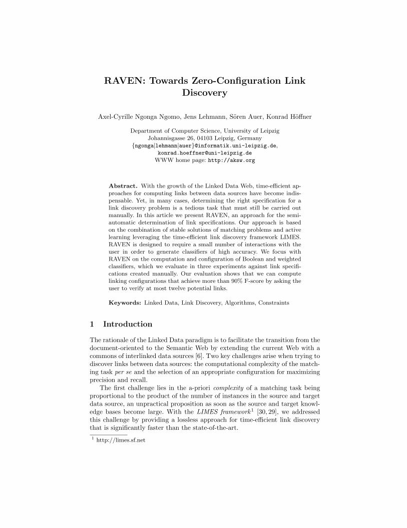
Algorithm 1 RAVEN’s stable matching algorithm

Require: Set of residents RRequire: Set of hospitals HRequire: Preference function p

M = ∅ // Mapping of hospitals to residentsfor r ∈ R doi(r) = 0 //index for preference function

end forfor h ∈ H doc(h) =

⌈|R||H|

⌉//capacity setting

end forwhile R 6= ∅ do

for r ∈ R doh = p(r)[i(r)]if |M(h)| < c(h) then

M(h) := M(h) ∪ {r}R = R\{r}

elseif ∃r′ ∈ M(h) p(h, r) < p(h, r′) thenr′′ = arg min

r′∈M(h)

p(h, r′)

R = R ∪ {r′′}M(h) := M(h)\{r′′}M(h) := M(h) ∪ {r}R = R\{r}

end ifend ifi(r) + +

end forend whilereturn M

Note that we assume there are no ties, i.e., that the functions µ and γ areinjective. Given these premises, [13] shows that a stable matching always exists.Consequently, Algorithm 1 is guaranteed to return a solution. Note that we setthe capacity of the hospitals to the smallest whole number that ensures that eachresident finds a hospital. Also note that p(h, r) < p(h, r′) means that h prefersr over r′. More details on stable matching can be found in [26].

3.3 Active Learning

Supervised batch learning approaches for learning classifiers must rely on largeamounts of labeled data to achieve a high accuracy. For example, the geneticprogramming approach used in [19] has been shown to achieve high accuracieswhen supplied with more than 1000 positive examples. The idea behind activelearning approaches (also called curious classifiers [40]) is to reduce the amountof labeled data needed for learning link specifications. This is carried out by

querying for the labels of chosen pairs (s, t) iteratively within the following three-step process: In a first step, we begin with an initial classifier C0. This classifieris usually derived by using either a rule of thumb (as in the case of RAVEN)or generated randomly (e.g., in genetic programming). During each iterationt ∈ N (step 2), we compute a set of k+ most informative positive resp. k− mostinformative negative examples (where k+, k− ∈ N). These are pairs (s, t)

1. whose classification is unknown,

2. which are classified as being links resp. not being links by the classifier atiteration and

3. which maximize an informativeness function.

In the case of linear classifiers, for example, the informativeness function is usu-ally the distance from a pair (s, t) to the boundary of the current classifier. Themost informative examples are presented to a human judge who provides theclassifier with the correct classification. This feedback is then used to update theclassifier. The iteration process is repeated until a termination condition suchas a maximal number of iterations, no further improvements within a certainnumber of iterations or a perfect match between the human judgement and theautomatic classification is reached (step 3). In the following, we present an ap-proach that implements these principles in detail. The reader is referred to [40]for more details on active learning.

4 The RAVEN Approach

Our approach, dubbed RAVEN (RApid actiVE liNking), addresses the task oflinking two knowledge bases S and T by using the active learning paradigmwithin the pool-based sampling setting [40]. Overall, the goal of RAVEN is tofind the best classifier C that achieves the highest possible precision, recall or F1

score as desired by the user. The algorithm also aims to minimize the burden onthe user by limiting the number of link candidates that must be labeled by theuser to a minimum.

Algorithm 2 The RApid actiVE liNking (RAVEN) algorithm

Require: Source knowledge base KS

Require: Target knowledge base KT

Find stable class matching between classes of KS and KT

Find stable property matching for the selected classesCompute sets S and T ; Create initial classifier C0; t := 0while termination condition not satisfied do

Ask the user to classify 2α examples; Update Ct to Ct+1; t := t+1end whileCompute set M of links between S and T based on Ct

return M

An overview of our approach is given in Algorithm 2. In a first step, RAVENaims to detect the restrictions that will define the sets S and T . To achieve thisgoal, it tries to find a stable matching of pairs of classes, whose instances areto be linked. This is done by applying a two-layered approach and generating asorted list of class mappings that are presented to the user, who can choose thepair that is to be matched. The second step of our approach consists of finding astable matching between the properties that describe the instances of the classesspecified in the first step. The user is also allowed to alter the suggested matchingat will. Based on the property mapping, we compute S and T and generate aninitial classifier C = C0 in the third step. We then refine C iteratively by askingthe user to classify pairs of instances that are most informative for our algorithm.C is updated until a termination condition is reached, for example Ct = Ct+1. Thefinal classifier is used to compute the links between S and T , which are returnedby RAVEN. In the following, we expand upon each of these three steps.

4.1 Stable Matching of Classes

The first component of a link specification is a set of restrictions that must befulfilled by the instances that are to be matched. We present herein how sucha matching can be carried out for restrictions that are of the form R(x) ↔x rdf:type someClass, as they are the most commonly used restriction. Weuse a two-layered approach for matching classes in knowledge bases. Our defaultapproach begins by selecting a user-specified number of sameAs links betweenthe source and the target knowledge base randomly. Then, it computes µ and γon the classes CS of KS and CT of KT as follows5:

µ(CS , CT ) = γ(CS , CT ) = |{s type Cs ∧ s sameAs t ∧ t type CT }|. (4)

Although several million sameAs links exist on the Web of Data, some knowledgebases that refer to the same entities do not share any links. Consequently, ourdefault approach fails when trying to process such pairs of knowledge bases. Inthis case, we run our fallback approach. It computes µ and γ on the classes of Sand T as follows:

µ(CS , CT ) = γ(CS , CT ) = |{s type Cs ∧ s p x ∧ t type CT ∧ t q x}|, (5)

where p and q can be any property. Hence, the similarity of two classes is com-puted as the number of property values shared by triples such that their subjectsare instances of CS resp. CT . Note that this similarity is independent from theproperties through which the instances are connected to the property values.

We can draw on stable matchings, as introduced in Section 3.2 in order to findthe most suitable pair of classes as follows: Let c(S) be the number of classes CSof S such that µ(CS , CT ) > 0 for any CT . Furthermore, let c(T ) be the numberof classes CT of T such that γ(CS , CT ) > 0 for any CS . The capacity of each CTis set to dc(S)/c(T )e, thus ensuring that the hospitals provide enough capacity

5 Note that we used type to denote rdf:type and owl:sameAs to denote sameAs.

to map all the possible residents. Once µ, γ and the capacity of each hospitalhas been set, we solve the equivalent HR problem. It is important to note thatalthough the functions µ and γ are equivalent in both our default and our fallbackapproaches, the resulting problem is not symmetric, i.e., p(CS , CT ) = ζ does notimply that p(CT , CS) = ζ.

After the HR problem has been solved, we present the user with a stablematching sorted in descending order relatively to µ(CS , CT ), thereby selectingthe pair with the highest µ(CS , CT ) as default match. Note that the fallbackapproach is approximately 30% slower than our default approach. Also, if thefallback approach fails, then we require the user to enter the class mappingmanually.

4.2 Stable Matching of Properties

The detection of the best matching pairs of properties is very similar to thecomputation of the best matching classes. For datatype properties p and q, weset:

µ(p, q) = γ(p, q) = {s type Cs ∧ s p x ∧ t type CT ∧ t q x}. (6)

Note that while this equation might appear to be the same as Equation 4, theyare actually different as p and q are bound in this equation. Thus, the similarityvalue that is computed is the number of common values that p and q link toand not (as in Equation 4) the number of common objects to triples whosesubjects are instances of CS resp. CT . The initial mapping of properties definesthe similarity space in which the link discovery task will be carried out. Notethat none of the prior approaches to active learning for record linkage or linkdiscovery automatized this step. We associate each of the basis vectors σi ofthe similarity space to exactly one of the pairs (p, q) of mapping propertiesdetected by RAVEN. Once the restrictions and the property mapping have beenspecified, we can fetch the elements of the sets S and T . Given S and T , we cannow compute an initial classifier that will be iteratively updated by RAVEN.

4.3 Initial Classifier

The specific formula for the initial linear weighted classifier L0 results from theformal model presented in Section 3 and is given by

FL0(s, t) =

n∑i=1

ω0i σi(s, t). (7)

Several initialization methods can be used for ω0i and the initial threshold τ0

of PL. Here we chose the use the simplest possible approach by setting ω0i := 1

and τ0 := κn, where κ ∈ [0, 1] is a user-specified threshold factor. Note thatsetting the overall threshold to κn is equivalent to stating that the arithmeticmean of the σi(s, t) must be equal to κ.

The equivalent initial Boolean classifier B0 is given by

FB0(s, t) =

n∧i=0

(σ0i (s, t) ≥ τ0i ) where τ0i := κ. (8)

4.4 Updating Classifiers

RAVEN follows an iterative update strategy, which consists of asking the user toclassify 2α elements of S × T (α is explained below) in each iteration step t andusing these to update the values of ωt−1i and τ t−1i computed at step t− 1. Themain requirements to the update approach is that it computes those elementsof S × T whose classification allow to maximize the convergence of Ct to a goodclassifier and therewith to minimize the burden on the user. The update strategyof RAVEN varies slightly depending on the family of classifiers. In the following,we present how RAVEN updates linear and Boolean classifiers.

Updating linear classifiers. The basic intuition behind our update approachis that given an initial classified L0, we aim to iteratively present the user withthose elements from S × T whose classification is most unsure until we reach acertain termination condition. An example of such an initial classifier is shownin Figure 1(a). We call the elements presented to the user examples. We call anexample positive when it is assumed by the classifier to belong to +. Else wecall it negative. In Figure 1, the elements that the classifier assigns to the class+ are drawn in violet, while the elements of − are drawn in orange. Once theuser has provided us with the correct classification for the examples presentedto him, the classifier can be updated effectively so as to better approximate thetarget classifier. In the following, we will define the notion of most informativeexample for linear classifiers before presenting our update approach.

When picturing a classifier as a boundary in the similarity space S thatseparates the classes + and −, the examples whose classification is most uncer-tain are obviously those elements from S × T who are closest to the boundaryspecified by the classifier at hand. Note that we must exclude examples thathave been classified previously, as presenting them to the user would not im-prove the classification accuracy of RAVEN while generating extra burden onthe user, who would have to classify the same link candidate twice. Figure 1(b)depicts the idea behind most informative examples for linear classifiers. The ele-ments of + and − that were not previously classified and that are closest to theboundary of L are selected as being most informative. These are the elementsthat are presented to the oracle (i.e., the user) for classification. An exampleof an oracle-given classification is given in Figure 1(c). The nodes marked witha + were marked by the user as being correct links, while those marked witha − were labeled as incorrect. Here, our classifier only classified one examplecorrectly. Given this information, we aim to generate a classifier that minimizethe overall error of RAVEN. To achieve this goal, we update the classifier byusing an approach derived from perceptron learning as shown in Figure 1(d).

(a) Initial classifier (b) Most informative positives and nega-tives

(c) Oracle results (d) Classifier update

(e) Most informative positives and nega-tives

(f) Termination

Fig. 1. Active learning as implemented by RAVEN. The most informative negativeand positive examples are marked with an “X”. The classified examples are markedwith “+” for positive and “-” for negative.

The basic intuition behind choosing perceptron learning over other approachesis that we assume that our classifier should not be altered too drastically aftereach iteration, a goal which can be achieved with this approach. We iterate thecomputation of the most informative positive and negative examples (see Fig-ure 1(e)) until a termination condition is reached, e.g., until the classifier canpredict the user classification correctly (see Figure 1(e)).

Formally, let Mt be the set of (s, t) ∈ S × T classified by Lt as belonging to+1. Furthermore, let Pt−1 (resp. N t−1) be the set of examples that have alreadybeen classified by the user as being positive examples, i.e, links (resp. negativeexamples, i.e., wrong links) in the first t−1 iterations. We define a set Λ as beinga set of most informative examples λ for Lt+1 when the following two conditionshold:

∀λ ∈ S × T (λ ∈ Λ→ λ /∈ Pt−1 ∪N t−1) (9)

∀λ′ /∈ Pt−1 ∪N t−1 : λ′ 6= λ→ |FLt(λ′)− τ t| ≥ |FLt(λ)− τ t|. (10)

Note that there are several sets of most informative examples of a given magni-tude. We denote a set of most informative examples of magnitude α by Λα. Aset of most informative positive examples, Λ+, is a set of pairs such that

∀λ /∈ Λ+∪Pt−1∪N t−1 : (FLt(λ) < τ t)∨(∀λ+ ∈ Λ+ : FLt(λ) > FLt(λ+)). (11)

In words, Λ+ is the set of examples that belong to class + according to C and areclosest to C’s boundary. Similarly, the set of most informative negative examples,Λ−, is the set of examples such that

∀λ /∈ Λ−∪Pt−1∪N t−1 : (FLt(λ) ≥ τ t)∨(∀λ− ∈ Λ− : FLt(λ) < FLt(λ−)). (12)

We denote a set of most informative (resp. negative) examples of magnitude αas Λ+

α (resp. Λ−α ). The 2α examples presented to the user consist of the unionΛ+α ∪ Λ−α , where Λ+

α and Λ−α are chosen randomly amongst the possible sets ofmost informative positive resp. negative examples .

The update rule for the weights of Lt is derived from the well-known Per-ceptron algorithm (see e.g., [36]), i.e.,

ωt+1i = ωti + η+

∑λ∈Λ+

ρ(λ)σi(λ)− η−∑λ∈Λ−

ρ(λ)σi(λ), (13)

where η+ is the learning rate for positives examples, η− is the learning rate fornegative examples and ρ(λ) is 0 when the classification of λ by the user and Ltare the same and 1 when they differ.

The threshold is updated similarly, i.e,

τ t+1i = τ ti + η+

∑λ∈Λ+

α

ρ(λ)FLt(λ)− η−∑λ∈Λ−α

ρ(λ)FLt(λ). (14)

Note that the weights are updated by using the dimension which they de-scribe while the threshold is updated by using the whole specific function. Finally,the sets Pt−1 and N t−1 are updated to

Pt := Pt−1 ∪ Λ+α (15)

andN t := N t−1 ∪ Λ−α . (16)

Updating Boolean classifiers The notion of most informative example differsslightly for Boolean classifiers. λ is considered a most informative example for Bwhen the conditions

λ /∈ Pt−1 ∪N t−1 (17)

and

∀λ′ /∈ Pt−1 ∪N t−1 : λ′ 6= λ→n∑i=1

|σti(λ′)− τ ti | ≥n∑i=1

|σti(λ)− τ ti | (18)

hold. The update rule for the thresholds τ ti of B is then given by

τ t+1i = τ ti + η+

∑λ∈Λ+

α

ρ(λ)σi(λ)− η−∑λ∈Λ−α

ρ(λ)σi(λ), (19)

where η+ is the learning rate for positives examples, η− is the learning rate fornegative examples and ρ(λ) is 0 when the classification of λ by the user and Ct−1are the same and 1 when they differ. The sets Pt−1 and N t−1 are updated asgiven in Equations 15 and 16.

5 Implementation

As stated above, RAVEN was implemented based on LIMES but the core ideaspresented herein can be implemented in any link discovery framework. Figure 2gives an overview of the workflow behind RAVEN. Once the classes and proper-ties have been matched, RAVEN begins by generating an initial classifier. Thisclassifier is converted into a link specification object that is forwarded to theLIMES kernel. The kernel then runs the link specification and generates a set ofpotential links with are sent back to RAVEN. RAVEN then computes the mostinformative positive and negative links and sends this set of inquiries to theoracle (i.e., the user). The oracle then classifies the links and sends the correctclassification back to RAVEN. If the classification has not been altered, RAVENterminates. Else the current classifier is updated and then transformed into alink specification, therewith starting the cycle anew. Note that the RAVEN al-gorithm is deterministic.

Classifier

Link Discovery

Framework (LIMES)

Most informative

examples

Oracle

Correct

classification

RAVEN

Update

Links

Link specification

Fig. 2. Workflow of the RAVEN implementation.

6 Experiments and Results

6.1 Experimental Setup

We carried out three series of experiments to evaluate our approach. In our firstexperiment, dubbed Diseases, we aimed to map diseases from DBpedia withdiseases from Diseasome. In the Drugs experiments, we linked drugs from Siderwith drugs from Drugbank. Here, only 43 links were to be detected. Finally, inthe Side-Effects experiments, we aimed to link side-effects of drugs and diseasesin Sider and Diseasome. The reference data consisted of 454 links. The size ofthe reference data is given in Table 1

Experiment S T |S| |T | Number of correct links

Diseases DBpedia Diseasome 4647 4213 178

Drugs Sider Drugbank 914 4772 43

Side-Effects Sider Diseasome 1737 4213 454Table 1. Overview of experimental data.

In all experiments, we aimed to compute how well linear and Boolean clas-sifiers learned by RAVEN could approximate a manually specified configurationfor mapping two knowledge bases. We used the following setup: The learningrates η+ and η− as explained in Section 4.4 were set to the same value η, whichwe varied between 0.01 and 0.1. We set the number of inquiries, i.e. the number ofquestions asked to the user, per iteration to 4. The threshold factor κ, explainedin Section 4.3 was set to 0.8. In addition, the number of instances used duringthe automatic detection of class resp. property matches was set to 100 resp. 500.If no class mapping was found via sameAs links, then the fallback solution wascalled and compared the property values of 1000 instances chosen randomly fromthe source and target knowledge bases. We used the trigrams metric as defaultsimilarity measure for strings and the Euclidean similarity as default similaritymeasure for numeric values. As reference data, we used the set of instances thatmapped perfectly according to a configuration created manually, which is simi-lar to the approach in [19]. We can then compute precision, recall and F-scoreagainst those reference links. We also measured the total number of inquiries,i.e. questions to the oracle, that RAVEN needed to reach its maximal F-score.All experiments were carried out on an Intel Core2 Duo computer with 2.53GHzand 3072MB RAM.

6.2 Results

Tables 2 and 3 present an excerpt of the mappings computed automatically byRAVEN. The elements of the stable matching computed from these mappingwere used as initial configuration. The results of our experiments are shown inFigures 3, 4 and 5. The first experiment, Diseases, proved to be the most difficult

Experiment Class Mapping

Diseases ds:diseases→dbp:Disease∗

ds:diseases→yago:Disease114070360

ds:diseases→yago:NeurologicalDisorders

ds:diseases→yago:TypesOfCancer

ds:diseases→yago:GeneticDisorders

ds:diseases→yago:BloodDisorders

ds:diseases→yago:TransmissibleSpongiformEncephalopathies

ds:diseases→yago:Syndromes

ds:diseases→yago:ChromosomeInstabilitySyndromes

ds:diseases→yago:PigmentDisorders

ds:diseases→yago:CongenitalDisorders

Drugs dbk:drugs→sd:drugs∗

dbk:drugs→sd:Offer

Side-Effects sd:sideEffects→ds:diseases∗

Table 2. Initial property and class mappings computed by RAVEN in our experiments.The class mappings marked with an asterisk were returned by the stable matchingalgorithm and used in the classifier.

Experiment Property Mapping

Diseases rdfs:label → dbp:name∗

rdfs:label → foaf:name

rdfs:label → rdfs:label

ds:name → dbp:name

ds:name → foaf:name∗

ds:name → rdfs:label

Drugs dbk:brandName → sd:drugName∗

dbk:genericName → sd:drugName

rdfs:label → sd:drugName

dbk:brandName → rdfs:label

Side-Effects rdfs:label → rdfs:label∗

rdfs:label → ds:name

sd:sideEffectName → rdfs:label

sd:sideEffectName → ds:name∗

Table 3. Initial property mappings computed by RAVEN in our experiments. Theproperty mappings marked with an asterisk were returned by the stable matchingalgorithm and used in the classifier.

for RAVEN. Although the sameAs links between Diseasome and DBpedia allowedour experiment to run without making use of the fallback solution, we had tosend 12 inquiries to the user when the learning rate was set to 0.1 to determinethe best configuration that could be learned by linear and Boolean classifiers.Smaller learning rates led to the system having to send even up to 80 inquiries (η= 0.01) to determine the best configuration. In this experiment linear classifiersoutperform Boolean classifiers in all setups by up to 0.8% F-score.

1 5 9 13 17 21 25

Number of iterations

30

40

50

60

70

80

90

100

F-Sc

ore

LR = 0.01LR = 0.02LR = 0.05LR = 0.1

(a) Linear classifier

1 5 9 13 17 21 25

Number of iterations

30

40

50

60

70

80

90

100

F-Sc

ore

LR = 0.01LR = 0.02LR = 0.05LR = 0.1

(b) Boolean classifier

Fig. 3. Learning curves on Diseases experiments.

The second and the third experiment display the effectiveness of RAVEN.Although the fallback solution had to be used in both cases, our approach isable to detect the right configuration with an accuracy of even 100% in theSide-Effects experiment by asking the user no more than 4 questions. This isdue to the linking configuration of the user leading to two well-separated sets ofinstances. In these cases, RAVEN converges rapidly and finds a good classifierrapidly. Note that in these two cases, all learning rates in combination with both

linear and Boolean classifiers led to the same results (see Figures 4 and 5). Theconfiguration learned for the Side-Effects experiment is shown in Figure 6.

1 5 9 13 17 21 25

Number of iterations

0

10

20

30

40

50

60

70

80

90

100

Precision (%)Recall (%)F-Score (%)

Fig. 4. Learning curve of the Drugs experiments.

1 5 9 13 17 21 25

Number of iterations

0

10

20

30

40

50

60

70

80

90

100

Precision (%)Recall (%)F-Score (%)

Fig. 5. Learning curve of the Side-Effect experiment.

Although we cannot directly compare our results to other approaches as it isthe first active learning algorithm for learning link specifications, results reportedin the database area suggest that RAVEN achieves state-of-the-art performance.The runtimes required for each iteration ensure that our approach can be usedin real-world interactive scenarios. In the worst case, the user has to wait for 1.4seconds between two iterations as shown in Figure 7. The runtime for the com-

1 <?xml version="1.0" encoding="UTF -8"?>2 <!DOCTYPE LIMES SYSTEM "limes.dtd">3 <LIMES>4 <PREFIX >5 <NAMESPACE >http: //www.w3.org /1999/02/22 -rdf -syntax -ns#</NAMESPACE >6 <LABEL>rdf</LABEL ></PREFIX >7 <PREFIX >8 <NAMESPACE >http: //www.w3.org /2000/01/rdf -schema#</NAMESPACE >9 <LABEL>rdfs</LABEL></PREFIX >

10 <PREFIX >11 <NAMESPACE >http://www.w3.org /2002/07/ owl#</NAMESPACE >12 <LABEL>owl</LABEL ></PREFIX >13 <PREFIX >14 <NAMESPACE >http://www4.wiwiss.fu-berlin.de/sider/resource/sider/</NAMESPACE >15 <LABEL>sd</LABEL></PREFIX >16 <PREFIX >17 <NAMESPACE >http://www4.wiwiss.fu-berlin.de/diseasome/resource/diseasome/18 </NAMESPACE >19 <LABEL>ds:</LABEL ></PREFIX >20 <SOURCE >21 <ID>sider</ID>22 <ENDPOINT >http://www4.wiwiss.fu-berlin.de/sider/sparql </ENDPOINT >23 <VAR>?x</VAR>24 <PAGESIZE >-1</PAGESIZE >25 <RESTRICTION >?x rdf:type sd:side_effects </RESTRICTION >26 <PROPERTY >rdfs:label </PROPERTY >27 <PROPERTY >sd:sideEffectName </PROPERTY >28 </SOURCE >29 <TARGET >30 <ID>diseasome </ID>31 <ENDPOINT >http://www4.wiwiss.fu-berlin.de/diseasome/sparql </ENDPOINT >32 <VAR>?y</VAR>33 <PAGESIZE >-1</PAGESIZE >34 <RESTRICTION >?y rdf:type ds:diseases </RESTRICTION >35 <PROPERTY >rdfs:label </PROPERTY >36 <PROPERTY >ds:name </PROPERTY >37 </TARGET >38 <METRIC >39 ADD (1.0083130081300813* Trigram(x.rdfs:label ,y.rdfs:label),40 1.0083130081300813* Trigram(x.sd:sideEffectName ,y.ds:name ))41 </METRIC >42 <ACCEPTANCE >43 <THRESHOLD >1.632</THRESHOLD >44 <FILE>sideEffects.ttl</FILE>45 <RELATION >owl:sameAs </RELATION >46 </ACCEPTANCE >47 <REVIEW >48 <THRESHOLD >1.632</THRESHOLD >49 <FILE>sideEffectsReview.ttl</FILE>50 <RELATION >owl:sameAs </RELATION >51 </REVIEW >52 <EXECUTION >Simple </EXECUTION >53 <GRANULARITY >4</GRANULARITY >54 <OUTPUT >TURTLE </OUTPUT >55 </LIMES>

Fig. 6. LIMES configuration learned for the Side-Effects experiment.

putation of the initial configuration depends heavily on the connectivity to theSPARQL endpoints. In our experiments, the computation of the initial configu-ration demanded 60 seconds when sameAs links existed between the knowledgebases. When the fallback solution was used, the runtimes increased and reached90 seconds.

1 3 5 7 9 11 13 15 17 19 21 23 25

Number of iterations

10

100

1000

Run

time

(ms)

DiseasesDrugsSide Effects

Fig. 7. Average runtimes for each iteration.

7 Conclusion and Future Work

In this paper, we presented RAVEN, an active learning approach tailored towardssemi-automatic link discovery on the Web of Data. We showed how RAVEN usesstable matching algorithms to detect initial link configurations. We opted to usethe solution of the hospital residence problem (HR) without ties because of thehigher time complexity of the solution of HR with ties, i.e., L4, where L is thesize of the longest preference list, i.e., max(|R|, |H|). Still, our work could beextended by measuring the effect of considering ties on the matching computedby RAVEN. Our experimental results showed that RAVEN can compute accu-rate link specifications (F-score between 90% and 100%) by asking the user toclassify a very small number of positive and negative examples (between 4 and12 for a learning rate of 0.1). Our results also showed that our approach can beused in an interactive scenario because of LIMES’ time efficiency, which allowedto compute new links in less than 1.5 seconds in the evaluation tasks. The ad-vantages of this interactive approach can increase the quality of generated linkswhile reducing the effort to create them. The RAVEN algorithm as well as agraphical user interface will be made available as open source within the SAIM6

framework.

6 http://saim.sf.net

In future work, we will explore how to detect optimal values for the thresholdfactor κ automatically, for example, by using clustering approaches. In addition,we will investigate the automatic detection of domain-specific metrics that canmodel the idiosyncrasies of the dataset at hand. Another promising extensionto RAVEN is the automatic detection of the target knowledge base to evenfurther simplify the linking process, since users often might not even be aware ofappropriate linking targets (see [16] for research in this area). By these means,we aim to provide the first zero-configuration approach to link discovery.

References

1. A. Arasu, M. Gotz, and R. Kaushik. On active learning of record matching pack-ages. In SIGMOD Conference, pages 783–794, 2010.

2. S. Araujo, J. Hidders, D. Schwabe, de Vries, and A. P. SERIMI - resource descrip-tion similarity, RDF instance matching and interlinking, July 06 2011.

3. S. Auer, J. Lehmann, and S. Hellmann. LinkedGeoData - adding a spatial dimen-sion to the web of data. In Proc. of 8th International Semantic Web Conference(ISWC), 2009.

4. Z. Bellahsene, A. Bonifati, and E. Rahm, editors. Schema Matching and Mapping.Springer, 2011.

5. M. Bilenko and R. J. Mooney. On evaluation and training-set construction forduplicate detection. In Proceedings of the KDD-2003 Workshop on Data Cleaning,Record Linkage, and Object Consolidation, pages 7–12, 2003.

6. C. Bizer, T. Heath, and T. Berners-Lee. Linked data - the story so far. InternationalJournal on Semantic Web and Information Systems (IJSWIS), 2009.

7. C. Bizer, J. Lehmann, G. Kobilarov, S. Auer, C. Becker, R. Cyganiak, and S. Hell-mann. DBpedia - a crystallization point for the web of data. Journal of WebSemantics, 2009.

8. J. Bleiholder and F. Naumann. Data fusion. ACM Comput. Surv., 41(1):1–41,2008.

9. P. Cudre-Mauroux, P. Haghani, M. Jost, K. Aberer, and H. de Meer. idmesh:graph-based disambiguation of linked data. In WWW, pages 591–600, 2009.

10. F. Duchateau, R. Coletta, Z. Bellahsene, and R. J. Miller. (not) yet anothermatcher. In Proceedings of the 18th ACM conference on Information and knowledgemanagement, CIKM ’09, pages 1537–1540, New York, NY, USA, 2009. ACM.

11. A. K. Elmagarmid, P. G. Ipeirotis, and V. S. Verykios. Duplicate record detection:A survey. IEEE Transactions on Knowledge and Data Engineering, 19:1–16, 2007.

12. J. Euzenat, A. Ferrara, C. Meilicke, J. Pane, F. Scharffe, P. Shvaiko, H. Stucken-schmidt, O. Svab-Zamazal, V. Svatek, and C. Trojahn. Results of the ontologyalignment evaluation initiative 2010. In Fifth International Workshop on OntologyMatching, pages 85–117, 2009.

13. D. Gale and L. S. Shapley. College admissions and the stability of marriage. TheAmerican Mathematical Monthly, 69(1):9–15, 1962.

14. H. Glaser, I. C. Millard, W.-K. Sung, S. Lee, P. Kim, and B.-J. You. Research onlinked data and co-reference resolution. Technical report, University of Southamp-ton, 2009.

15. M. Granitzer, V. Sabol, K. W. Onn, D. Lukose, and K. Tochtermann. Ontologyalignment - A survey with focus on visually supported semi-automatic techniques.Future Internet, 2(3):238–258, 2010.

16. C. Gueret, P. Groth, F. van Harmelen, and S. Schlobach. Finding the achilles heelof the web of data: Using network analysis for link-recommendation. In ISWC,pages 289–304, 2010.

17. A. Hogan, A. Polleres, J. Umbrich, and A. Zimmermann. Some entities are moreequal than others: statistical methods to consolidate linked data. In NeFoRS, 2010.

18. W. Hu, J. Chen, G. Cheng, and Y. Qu. Objectcoref & falcon-AO: results for OAEI2010. In P. Shvaiko, J. Euzenat, F. Giunchiglia, H. Stuckenschmidt, M. Mao,and I. F. Cruz, editors, OM, volume 689 of CEUR Workshop Proceedings. CEUR-WS.org, 2010.

19. R. Isele and C. Bizer. Learning linkage rules using genetic programming. InP. Shvaiko, J. Euzenat, T. Heath, C. Quix, M. Mao, and I. F. Cruz, editors, OM,volume 814 of CEUR Workshop Proceedings. CEUR-WS.org, 2011.

20. H. Kopcke and E. Rahm. Training selection for tuning entity matching. In QD-B/MUD, pages 3–12, 2008.

21. H. Kopcke, A. Thor, and E. Rahm. Comparative evaluation of entity resolutionapproaches with fever. Proc. VLDB Endow., 2(2):1574–1577, 2009.

22. Y. Lee, M. Sayyadian, A. Doan, and A. Rosenthal. etuner: tuning schema matchingsoftware using synthetic scenarios. VLDB J., 16(1):97–122, 2007.

23. U. Leser and F. Naumann. Informationsintegration - Architekturen und Methodenzur Integration verteilter und heterogener Datenquellen. dpunkt.verlag, 2007.

24. V. I. Levenshtein. Binary codes capable of correcting deletions, insertions, andreversals. Technical Report 8, 1966.

25. J. Li, J. Tang, Y. Li, and Q. Luo. RiMOM: A dynamic multistrategy ontologyalignment framework. IEEE Trans. Knowl. Data Eng, 21(8):1218–1232, 2009.

26. D. Manlove, R. Irving, K. Iwama, S. Miyazaki, and Y. Morita. Hard variants ofstable marriage. Theoretical Computer Science, 276(1-2):261 – 279, 2002.

27. A. Marie and A. Gal. Boosting schema matchers. In Proceedings of the OTM 2008Confederated International Conferences, CoopIS, DOA, GADA, IS, and ODBASE2008. Part I on On the Move to Meaningful Internet Systems:, OTM ’08, pages283–300, Berlin, Heidelberg, 2008. Springer-Verlag.

28. M. Morsey, J. Lehmann, S. Auer, C. Stadler, and S. Hellmann. DBpedia and theLive Extraction of Structured Data from Wikipedia. Program: electronic libraryand information systems, 46:27, 2012.

29. A.-C. Ngonga Ngomo. A time-efficient hybrid approach to link discovery. InProceedings of OM@ISWC, 2011.

30. A.-C. Ngonga Ngomo and S. Auer. Limes - a time-efficient approach for large-scalelink discovery on the web of data. In Proceedings of IJCAI, 2011.

31. A.-C. Ngonga Ngomo, J. Lehmann, S. Auer, and K. Hffner. Raven – active learningof link specifications. In Proceedings of OM@ISWC, 2011.

32. A. Nikolov, V. S. Uren, E. Motta, and A. N. D. Roeck. Overcoming schema het-erogeneity between linked semantic repositories to improve coreference resolution.In ASWC, pages 332–346, 2009.

33. G. Papadakis, E. Ioannou, C. Niedere, T. Palpanasz, and W. Nejdl. Eliminatingthe redundancy in blocking-based entity resolution methods. In JCDL, 2011.

34. E. Rahm and P. A. Bernstein. A survey of approaches to automatic schema match-ing. VLDB J., 10(4):334–350, 2001.

35. Y. Raimond, C. Sutton, and M. Sandler. Automatic interlinking of music datasetson the semantic web. In Proceedings of the 1st Workshop about Linked Data onthe Web, 2008.

36. R. Rojas. Neural Networks: A Systematic Introduction. Springer, 1 edition, July1996.

37. S. Sarawagi and A. Bhamidipaty. Interactive deduplication using active learning.In KDD, pages 269–278, 2002.

38. S. Sarawagi, A. Bhamidipaty, A. Kirpal, and C. Mouli. Alias: An active learningled interactive deduplication system. In VLDB, pages 1103–1106, 2002.

39. F. Scharffe, Y. Liu, and C. Zhou. Rdf-ai: an architecture for rdf datasets matching,fusion and interlink. In Proc. IJCAI 2009 workshop on Identity, reference, andknowledge representation (IR-KR), Pasadena (CA US), 2009.

40. B. Settles. Active learning literature survey. Technical Report 1648, University ofWisconsin-Madison, 2009.

41. J. Sleeman and T. Finin. Computing foaf co-reference relations with rules andmachine learning. In Proceedings of SDoW, 2010.

42. C. Stadler, J. Lehmann, K. Hoffner, and S. Auer. Linkedgeodata: A core for a webof spatial open data. Semantic Web Journal, 3(4):333–354, 2012.

43. C. Stadler, M. Martin, J. Lehmann, and S. Hellmann. Update Strategies for DB-pedia Live. In 6th Workshop on Scripting and Development for the Semantic WebColocated with ESWC 2010 30th or 31st May, 2010 Crete, Greece, 2010.

44. W. R. van Hage. Evaluating Ontology-Alignment Techniques. PhD thesis, VrijeUniversiteit Amsterdam, 2008.

45. J. Volz, C. Bizer, M. Gaedke, and G. Kobilarov. Discovering and maintaining linkson the web of data. In ISWC, pages 650–665, 2009.

46. W. Winkler. Overview of record linkage and current research directions. Technicalreport, Bureau of the Census - Research Report Series, 2006.