FEDERAL RESERVE BANK OF SAN FRANCISCO

WORKING PAPER SERIES

Working Paper 2007-10 http://www.frbsf.org/publications/economics/papers/2007/wp07-10bk.pdf

The views in this paper are solely the responsibility of the authors and should not be interpreted as reflecting the views of the Federal Reserve Bank of San Francisco or the Board of Governors of the Federal Reserve System.

Rational and Near-Rational Bubbles Without Drift

Kevin J. Lansing Federal Reserve Bank of San Francisco

October 2009

Rational and Near-Rational Bubbles Without Drift�

Kevin J. Lansingy

Federal Reserve Bank of San Francisco

October 8, 2009

Abstract

This paper derives a general class of intrinsic rational bubble solutions in a Lucas-typeasset pricing model. I show that the rational bubble component of the price-dividendratio can evolve as a geometric random walk without drift, such that the mean of thebubble growth rate is zero. Driftless bubbles are part of a continuum of equilibriumsolutions that satisfy a period-by-period no-arbitrage condition. I also derive a near-rational solution in which the agent�s forecast rule is under-parameterized. The near-rational solution generates intermittent bubbles and other behavior that is quantitativelysimilar to that observed in long-run U.S. stock market data.

Keywords: Asset Pricing, Rational Bubbles, Excess Volatility, Learning.

JEL Classi�cation: E44, G12.

�Forthcoming, Economic Journal. For helpful comments and suggestions, I would like to thank Eric En-gstrom, Steve LeRoy, Kjersti-Gro Lindquist, participants at the 2007 Meeting of the Society for EconomicDynamics, the 2007 Meeting of the Society for Computational Economics, the 2007 Meeting of the Society forNonlinear Dynamics and Econometrics, and the 2008 Norges Bank Symposium on Fundamental and Nonfun-damental Asset Price Dynamics. I also thank two anonymous referees for thoughtful suggestions that improvedthe paper.

y Research Department, Federal Reserve Bank of San Francisco, P.O. Box 7702, San Francisco,CA 94120-7702, (415) 974-2393, FAX: (415) 977-4031, email: kevin.j.lansing@sf.frb.org, homepage:www.frbsf.org/economics/economists/klansing.html

Nowhere does history indulge in repetitions so often or so uniformly as in WallStreet. When you read contemporary accounts of booms or panics the one thing thatstrikes you most forcibly is how little either stock speculation or stock speculatorstoday di¤er from yesterday. The game does not change and neither does humannature.From the thinly-disguised biography of legendary speculator Jesse Livermore,

by E. Lefevére (1923, p. 180).

1 Introduction

Stories involving speculative bubbles can be found throughout history in various countries andasset markets.1 The dramatic rise in U.S. stock prices during the late 1990s, followed similarlyby U.S. house prices during the mid 2000s, are episodes that have both been described asbubbles. The term �bubble�was coined in England in 1720 following the famous price run-upand crash of shares in the South Sea Company. The run-up led to widespread public enthusiasmfor the stock market and a proliferation of highly suspect companies attempting to sell sharesto investors. One such venture notoriously advertised itself as �a company for carrying out anundertaking of great advantage, but nobody to know what it is.�The epidemic of fraudulentstock-o¤ering schemes led the British government to pass the so-called �Bubble Act�in 1720,which was o¢ cially named �An Act to Restrain the Extravagant and Unwarrantable Practiceof Raising Money by Voluntary Subscription for Carrying on Projects Dangerous to the Tradeand Subjects of the United Kingdom.�2

Numerous empirical studies starting with Shiller (1981) and LeRoy and Porter (1981) havedemonstrated that stock prices appear to exhibit �excess volatility�when compared to thediscounted stream of ex post realized dividends.3 Bubble models o¤er a potential explanationfor excess volatility because they allow stock prices to become detached from fundamentals.So-called �rational bubble�models say that agents are fully cognizant of the fundamental assetprice, but nevertheless they may be willing to pay more than this amount. This can occurif expectations of future price appreciation are large enough to satisfy the rational agents�srequired rate of return. In the typical rational bubble model, the stock price grows faster thandividends (or cash �ows) in perpetuity, i.e., the price-dividend ratio exhibits positive drift. Thisis clearly an unrealistic prediction for long-run stock market behavior. Indeed, Hall (2001, p.3) dismisses the idea that �intelligent people [would] believe that the value of a stock willbecome larger and larger in relation to all other quantities in the economy.�A more elaboratemodel assumes that the bubble will periodically crash according to some universally knownprobability function, but this is an ad hoc feature that is determined completely outside ofthe model.4 Notwithstanding these criticisms, LeRoy (2004, p.784) maintains that �[rational]bubbles are a viable candidate for an explanation for the volatility of asset prices, even if it is

1See, for example, the collection of papers in Hunter, Kaufman, and Pomerleano (2003).2See Gerding (2006).3Shiller (2003) provides an update on this literature.4Rational bubble models with exogenous crash probablities include Blanchard (1979), Blanchard and Watson

(1982), Evans (1991), Fukata (1998), and Van Norden and Schaller (1999), among others.

1

not entirely clear how bubbles should be modeled.�This paper derives a rational bubble solution that is less susceptible to some of the above

criticisms. The framework for the analysis is a standard Lucas (1978) type asset pricingmodel. For any given value of risk aversion, I show that there are two distinct rational bubblesolutions for which the bubble component of the price-dividend ratio evolves as a geometricrandom walk without drift, such that the unconditional mean of the bubble growth rate is zero.Under each solution, the volatility of bubble innovations depends exclusively on fundamentals,i.e., the bubble is �intrinsic� in the terminology of Froot and Obstfeld (1991). Starting froman arbitrarily small positive value, a driftless rational bubble expands and contracts overtime in a irregular, wholly endogenous fashion. Although the price-dividend ratio remainsnon-stationary, the equilibrium trajectory is less explosive than a bubble with positive drift.I show that driftless rational bubbles are part of a continuum of equilibrium solutions thatsatisfy a period-by-period no-arbitrage condition. The positive-drift bubble solution derivedby Froot and Obstfeld (1991) can be recovered as a special case along this continuum.

Rational bubble models assume that agents always know the size of the bubble� to thepoint of constructing separate forecasts for the fundamental and bubble components of theasset price. An agent with limited computational resources may be inclined to construct only asingle forecast that predicts the movement of the total asset price (fundamental plus bubble).As noted by Nerlove (1983, p. 1255): �Purposeful economic agents have incentives to eliminateerrors up to a point justi�ed by the costs of obtaining the information necessary to do so.�Furthermore, rational bubble models are silent on how agents would coordinate on a particularrational bubble solution among a continuum of available solutions. To address such concerns,I solve for a near-rational equilibrium in which the agent�s forecast rule for the total assetprice is based on a geometric random walk without drift. The innovations to the random walkare linked to observable fundamentals, namely, consumption/dividend growth. The agent�sforecast rule is similar in form to the corresponding rational forecast, but it involves fewerparameters. The parameters of the agent�s forecast rule are chosen to match the moments ofobservable data. Using a real-time learning algorithm, I demonstrate that the near-rationalsolution is learnable.

The actual law of motion for the near-rational price-dividend ratio turns out to be station-ary, highly persistent, and nonlinear. The agent�s forecast errors exhibit near-zero autocorre-lation at all lags, making it di¢ cult for the agent to detect a misspeci�cation of the subjectiveforecast rule. Unlike a rational bubble, the near-rational solution allows the asset price tooccasionally dip below its fundamental value. Under mild risk aversion, the near-rationalsolution generates pronounced low-frequency swings in the price-dividend ratio, positive skew-ness, excess kurtosis, and time-varying volatility� all of which are present in long-run U.S.stock market data.

An additional contribution of the paper is to demonstrate an approximate analytical solu-tion for the fundamental asset price that employs a nonlinear change of variables. The behaviorof the changed variable is well-captured by a simple exponential function, as opposed to thehigh-order polynomial function employed in the approximate solution derived by Calin, et. al(2005). I show that the exponential approximation yields results that are very close to the

2

exact theoretical solution derived by Burnside (1998) for the case of autocorrelated dividendgrowth.

The near-rational asset pricing solution developed here is related to a large body of researchthat seeks to explain stock market behavior using some type of distorted belief mechanismor misspeci�ed forecast rule in a representative agent framework. Examples along these linesinclude Barsky and Delong (1993), Timmerman (1996), Barberis, Shleifer, and Vishney (1998),Cecchetti, Lam, and Mark (2000), Abel (2002), Lansing (2006, 2009), Branch and Evans(forthcoming), and Bullard, Evans, and Honkapohja (forthcoming), among others. Bubblemodels that involve the interaction of rational and non-rational agents in the same economyinclude Delong et al. (1990), Brock and Hommes (1998), Abreu and Brunnermeier (2003),and Scheinkman and Xiong (2003).

Another related paper in one by Adam, Marcet, and Nicolini (2008), who also develop anear-rational asset pricing solution. The authors introduce bounded-rationality in the form oflearning to account for several quantitative features of U.S. stock market data, including thehigh volatility and persistence of the price-dividend ratio. In their model, the representativeagent constructs separate forecasts for dividend growth and for price growth. The agent hasrational expectations regarding dividend growth, but the agent employs a momentum-basedforecast rule for price growth. Given su¢ cient data, the learning algorithm for price growtheventually converges to the fundamental solution. In contrast, I consider a solution where theagent constructs a forecast for a composite variable that depends on both prices and dividends.The functional form of the agent�s forecast rule is motivated by the form of the driftless rationalbubble solution. Since the agent�s forecast rule does not nest the fundamental solution as aspecial case, the long-run equilibrium continues to exhibit excess volatility.

The paper is organized as follows. First, I describe the model and the approximate funda-mental solution. I then demonstrate the existence of a continuum of nonstationary, intrinsicrational bubble solutions and highlight some special cases along the continuum. Next, I de-velop a stationary, near-rational asset pricing solution that involves a parsimonious forecastrule which is parameterized by matching the moments of observable data. Finally, using nu-merical simulations, I show that the near-rational solution performs well in matching featuresof long-run U.S. stock market data.

2 The Model

Equity shares are priced using the frictionless pure exchange model of Lucas (1978). There isa representative agent who can purchase shares to transfer wealth from one period to another.Each share pays an exogenous stream of stochastic dividends in perpetuity.

The agent�s problem is to maximize

E0

1Xt=0

�t�c1��t � 11� �

�; (1)

subject to the budget constraint

ct + ptst = (pt + dt) st�1; ct; st � 0 (2)

3

where ct is the agent�s consumption in period t; � is the subjective time discount factor,and � is the coe¢ cient of relative risk aversion (the inverse of the intertemporal elasticity ofsubstitution). When � = 1; the within-period utility function can be written as log (ct) : Thesymbol Et represents the mathematical expectation operator evaluated using the objectivedistribution of dividend growth. The symbol pt denotes the ex-dividend price of the equityshare, dt is the dividend, and st is the number of shares held in period t:

The growth rate of dividends xt � log (dt=dt�1) is governed by the following stochasticprocess

xt = x+ � (xt�1 � x) + "t; "t � N�0; �2"

�; (3)

where j�j < 1: The mean growth rate is x and the variance is �2"=(1� �2).The �rst-order condition that governs the agent�s share holdings is given by

pt = Et

"�

�ct+1ct

���(pt+1 + dt+1)

#: (4)

Equation (4) can be rearranged to obtain

1 = Et [Mt+1Rt+1] ; (5)

where Mt+1 � � (ct+1=ct)�� is the stochastic discount factor and Rt+1 = (pt+1 + dt+1) =pt isthe gross return from holding the equity share from period t to t+1: De�ning the price-dividendratio as yt � pt=dt; the gross equity return can be written as

Rt+1 =

�yt+1 + 1

yt

�exp (xt+1) : (6)

Following Lucas (1978), equity shares are assumed to exist in unit net supply. Marketclearing therefore implies st = 1 for all t: Substituting this equilibrium condition into thebudget constraint (2) yields, ct = dt for all t: In equilibrium, equation (4) can now be writtenas

yt = Et [� exp (�xt+1) (yt+1 + 1)] ; (7)

where � � 1 � �: Equation (7) shows that the price-dividend ratio in period t depends onthe agent�s joint forecast of next period�s dividend growth rate xt+1 and next period�s price-dividend ratio yt+1: It is convenient to transform equation (7) using a nonlinear change ofvariables to obtain

zt = � exp (�xt) [Etzt+1 + 1] ; (8)

where zt � � exp (�xt) (yt + 1) : Under this formulation, zt represents a composite variablethat depends on both the growth rate of dividends and the price-dividend ratio. Equation (8)shows that the value of zt in period t depends on the agent�s conditional forecast of that samevariable. By making use of the de�nition of zt; equation (7) can be written as yt = Etzt+1:

Hence, the equilibrium price-dividend ratio is simply the conditional forecast of the compositevariable zt+1:5

5The appendix outlines a version of the model that allows ct 6= dt:

4

3 Fundamental Solution

The fundamental value of the share price is uniquely pinned down by the agent�s rationalforecast of the discounted stream of future dividends. Equation (8) can be iterated forward tosubstitute out zt+1+k for k = 0; 1; 2; ::: Applying the law of iterated expectations and imposinga transversality condition yields the following present-value pricing equation

zft = � exp (�xt)Et�1 + � exp (�xt+1) + �2 exp (�xt+1 + �xt+2) +

�3 exp (�xt+1 + �xt+2 + �xt+3) :::; (9)

where zft is the fundamental value of the composite forecast variable. Following Burnside(1998), the expectation of the in�nite sum in (9) can be explicitly evaluated to yield thefollowing exact analytical solution

zft = � exp (�xt)

(1 +

1Xi=1

�i exp [�i + i (xt � x)]); (10)

�i = �xi+�2�2"

2 (1� �2)

"i�

2��1� �i

�1� � +

�2�1� �2i

�1� �2

#; (11)

i =���1� �i

�1� � : (12)

Given zft ; we can recover the fundamental price-dividend ratio by applying the de�nitionalrelationship yft = ��1 exp (��xt) zft � 1: This procedure yields the result that yft is equal tothe in�nite sum inside the curly brackets in equation (10). In the special case when � = 0; wehave i = 0 such that y

ft is constant.

6

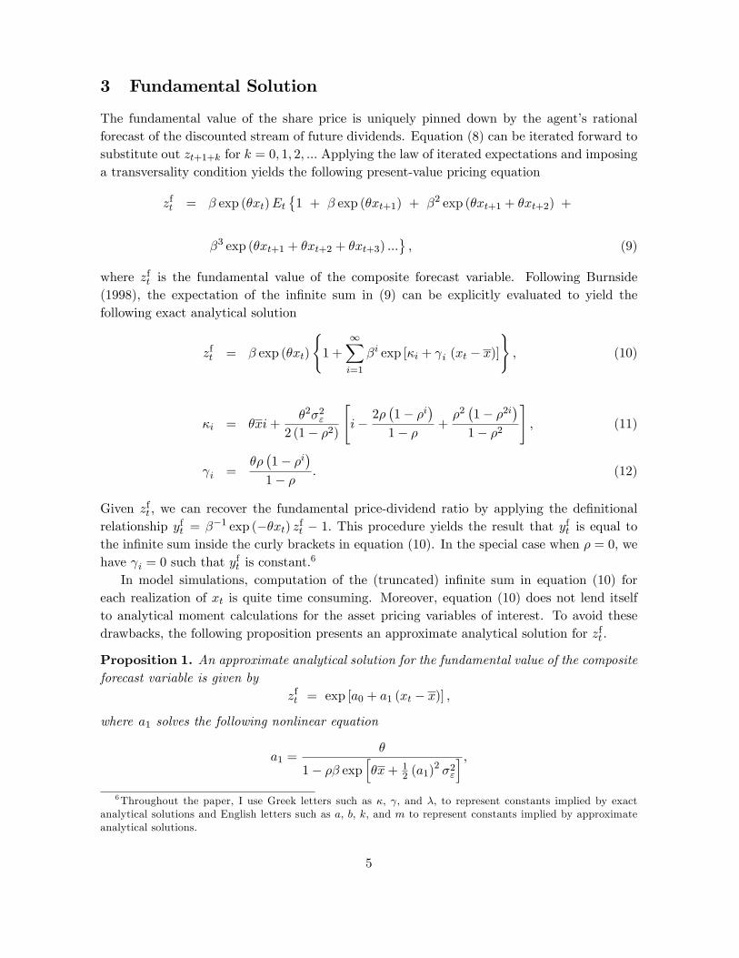
In model simulations, computation of the (truncated) in�nite sum in equation (10) foreach realization of xt is quite time consuming. Moreover, equation (10) does not lend itselfto analytical moment calculations for the asset pricing variables of interest. To avoid thesedrawbacks, the following proposition presents an approximate analytical solution for zft :

Proposition 1. An approximate analytical solution for the fundamental value of the compositeforecast variable is given by

zft = exp [a0 + a1 (xt � x)] ;

where a1 solves the following nonlinear equation

a1 =�

1� �� exph�x+ 1

2 (a1)2 �2"

i ;6Throughout the paper, I use Greek letters such as �; ; and �; to represent constants implied by exact

analytical solutions and English letters such as a; b; k; and m to represent constants implied by approximateanalytical solutions.

5

and a0 � E�log�zft��is given by

a0 = log

8<: � exp (�x)

1� � exph�x+ 1

2 (a1)2 �2"

i9=; ;

provided that 1 > � exph�x+ 1

2 (a1)2 �2"

i:

Proof : See appendix.

Two values of a1 satisfy the nonlinear equation. The inequality restriction selects the valueof a1 with lower magnitude to ensure that the point of approximation exp (a0) is positive: Theapproximate solution in Proposition 1 is much simpler in structure than the one derived byCalin, et. al (2005) for their corresponding model with no habit formation. These authorsnumerically approximate the law of motion of the changed variable qft � exp (���xt) yft usinga polynomial of the form�

dtdt�1

���(1��)�pftdt

�| {z }

qft

= ba0 + 8Xi=1

bai (xt � x)i ; (13)

which involves a total of nine Taylor-series coe¢ cients.7 In contrast, Proposition 1, analyticallyapproximates the law of motion of the changed variable zft � � exp (�xt)

�yft + 1

�using the

exponential form

�

�dtdt�1

�1���pftdt+ 1

�| {z }

zft

= exp [a0 + a1 (xt � x)] ; (14)

which involves only two Taylor-series coe¢ cients, a0 and a1: The approximation in Proposi-tion 1 exploits the curvature of the exponential function rather than relying on a high-orderpolynomial in (xt � x) to capture curvature.

We can recover an approximate solution for the fundamental price-dividend ratio by ap-plying the equilibrium relationship yft = Etz

ft+1; yielding

yft = Etzft+1 = exp

�a0 + a1� (xt � x) +

1

2(a1)

2 �2"

�: (15)

The above equation illustrates why it is di¢ cult for the fundamental solution to capture thehigh volatility and persistence of the price-dividend ratio observed in the data. The equationshows that yft will be constant if either a1 or � is equal to zero. Proposition 1 shows that a1will be close to zero for risk coe¢ cients near unity, representing logarithmic utility. The valueof � is pinned down by the autocorrelation of consumption growth, which is also close to zeroin long-run U.S. data. To generate high volatility and persistence in yft ; the model requiresa large risk coe¢ cient combined with a persistent process for consumption/dividend growth.

7See Calin, et. al (2005), Table 1, p. 977.

6

Alternatively, volatility and persistence in the model can be magni�ed by allowing deviationsfrom full-rationality. For example, Barsky and Delong (1993) assume that agents construct atime-varying estimate of the parameter x using an exponentially-weighted moving average ofpast observed growth rates. They show that the perception of shifting mean growth rates cangenerate long swings in the model price-dividend ratio.

Figure 1 compares the approximate and exact analytical solutions for two di¤erent cal-ibrations of the model. Throughout the paper, the agent�s discount factor is set equal to� = 0:958; a reasonable value for annual time periods. In panel (a), the risk coe¢ cient isset equal to � = 1:5 and the consumption growth process is calibrated to match the mean,standard deviation, and �rst-order autocorrelation of U.S. annual data for the growth of realper capita consumption of nondurables and services from 1890 to 2004.8 This procedure yieldsx = 0:0206; �" = 0:0354; and � = �0:1: In panel (b), the risk coe¢ cient is increased to � = 10while the persistence parameter for consumption growth is increased to � = 0:5; with the valueof �" adjusted downward to maintain the same volatility of consumption growth as in panel(a).

In panel (a) of Figure 1, the approximate solution is virtually indistinguishable from theexact fundamental solution. For this calibration, the standard deviation of the fundamentalprice dividend ratio is tiny� only 0.03 versus a whopping 13.8 in long-run U.S. data. In panel(b), where the model calibration is less plausible, the price dividend ratio is more volatile, butstill well below the U.S. value. In this case, the approximate solution is somewhat less accurate,exhibiting a root mean squared percentage error of 7.8 %. Collard and Juillard (2001) also �ndthat approximation errors increase with risk aversion and the persistence of the consumptiongrowth process. A more accurate approximation could be obtained by increasing the orderof the polynomial that appears inside the exponential function on the right-side of equation(14). Experiments with the model show that a quadratic polynomial inside the exponential issuccessful in reducing the approximation error to nearly zero for the calibration of panel (b).

As shown in the appendix, the approximate fundamental solution can be used to derivethe following expressions for the unconditional moments of the asset pricing variables

Ehlog�yft

�i= a0 +

12 (a1)

2 �2"; (16)

V arhlog�yft

�i=(a1�)

2 �2"1� �2 ; (17)

Ehlog�Rft+1

�i= � log (�) + �x � 1

2 (a1)2 �2", (18)

V arhlog�Rft+1

�i=

��2

1� �2 + (a1)2 + 2�a1

��2": (19)

Given equations (16) through (19), the unconditional moments of yft and Rft+1 can be computed

8Long-run annual data for U.S. consumption and U.S. stock market variables are from Robert Shiller�swebsite: http://www.econ.yale.edu/~shiller/.

7

by making use of the properties of the log-normal distribution.9

4 Rational Bubble Solutions

The present-value pricing equation (9) imposes a no-arbitrage condition across all future timeperiods whereas equation (8) imposes a no-arbitrage condition only from period t to t + 1:Since equation (8) does not enforce a transversality condition, it admits solutions where zt candeviate from the fundamentals-based value. These so-called �rational bubble�solutions havebeen proposed as a way to account for the empirical observation that stock prices appear to beexcessively volatile relative to a discounted stream of dividends or cash �ows. The underlyingassumption is that agents are forward-looking, but not to the extreme degree implied by thetransversality condition.

Tirole (1982, 1985), Santos and Woodford (1997), Kamigashi (1998), and Montrucchioand Pivileggi (2001) all discuss the many theoretical caveats that govern the existence ofrational bubbles in an intertemporal competitive equilibrium. A basic intuition is that rationalbubbles can usually be ruled out for the simple reason that, if a bubble existed, then anin�nitely-lived agent could achieve a gain by permanently selling shares at the bubble priceand then foregoing dividends on those shares. Since the rational bubble solution assumesst = 1 for all t; the solution fails to maximize in�nite-horizon utility as implicitly requiredby the rational equilibrium concept. In light of such arguments, the term �rational bubble�should perhaps be considered a misnomer. Nevertheless, so-called rational bubbles can still beviewed as a possible descriptive model of asset pricing, even if these solutions do not maximizein�nite-horizon utility. Along these lines, LeRoy (2004, p. 801), remarks �It is a testament toeconomists�capacity for abstraction that they have accepted without question that an intricatetheoretical argument against bubbles has somehow migrated from the pages of Econometricato the �oor of the New York Stock Exchange.�

The forecast variable zt that appears in equation (8) can be disaggregated as follows

zt = zft + zbt ; (20)

where zft satis�es the present-value pricing equation (9) and hence also satis�es (8). The bubblecomponent of the forecast variable is de�ned as zbt � � exp (�xt) y

bt ; where y

bt is the bubble

component of the price-dividend ratio. Substituting equation (20) into (8) yields the followingexpectational di¤erence equation that governs the evolution of the bubble component

zbt = � exp (�xt)Etzbt+1: (21)

Together, equations (8) and (21) imply

Etzt+1| {z }yt

= Etzft+1| {z }yft

+ Etzbt+1| {z }ybt

; (22)

which shows that Etzt+1 is the sum of two separate forecasts that pertain to the fundamentaland bubble components, respectively.

9 If a random variable wt is log-normally distributed, then E (wt) = exp�E [log (wt)] +

12V ar [log (wt)]

and

V ar (wt) = E (wt)2 fexp (V ar [log (wt)])� 1g :

8

4.1 Continuum of Intrinsic Rational Bubbles

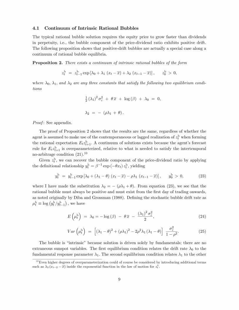
The typical rational bubble solution requires the equity price to grow faster than dividendsin perpetuity, i.e., the bubble component of the price-dividend ratio exhibits positive drift.The following proposition shows that positive-drift bubbles are actually a special case along acontinuum of rational bubble equilibria.

Proposition 2. There exists a continuum of intrinsic rational bubbles of the form

zbt = zbt�1 exp [�0 + �1 (xt � x) + �2 (xt�1 � x)] ; zb0 > 0;

where �0; �1; and �2 are any three constants that satisfy the following two equilibrium condi-tions

12 (�1)

2 �2" + � x + log (�) + �0 = 0;

�2 = � (��1 + �) :

Proof : See appendix.

The proof of Proposition 2 shows that the results are the same, regardless of whether theagent is assumed to make use of the contemporaneous or lagged realization of zbt when formingthe rational expectation Etzbt+1: A continuum of solutions exists because the agent�s forecastrule for Etzbt+1 is overparameterized, relative to what is needed to satisfy the intertemporalno-arbitrage condition (21).10

Given zbt ; we can recover the bubble component of the price-dividend ratio by applyingthe de�nitional relationship ybt = �

�1 exp (��xt) zbt ; yielding

ybt = ybt�1 exp [�0 + (�1 � �) (xt � x)� ��1 (xt�1 � x)] ; yb0 > 0; (23)

where I have made the substitution �2 = � (��1 + �). From equation (23), we see that therational bubble must always be positive and must exist from the �rst day of trading onwards,as noted originally by Diba and Grossman (1988). De�ning the stochastic bubble drift rate as�bt � log

�ybt =y

bt�1�; we have

E��bt

�= �0 = � log (�) � � x � (�1)

2 �2"2

; (24)

V ar��bt

�=h(�1 � �)2 + (��1)2 � 2�2�1 (�1 � �)

i �2"1� �2 : (25)

The bubble is �intrinsic�because solution is driven solely by fundamentals; there are noextraneous sunspot variables. The �rst equilibrium condition relates the drift rate �0 to thefundamental response parameter �1: The second equilibrium condition relates �1 to the other

10Even higher degrees of overparameterization could of course be considered by introducing additional termssuch as �3 (xt�2 � x) inside the exponential function in the law of motion for zbt :

9

fundamental response parameter �2: If �0 � 0, the magnitude of �1 must be larger to satisfythe �rst equilibrium condition. Intuitively, an increase in the magnitude of �1 raises the valueof Etzbt+1 via Jensen�s inequality, thereby allowing equation (21) to be satis�ed with a zero ornegative drift rate.

4.2 Special Cases

If we impose an arbitrary restriction on either �0; �1; or �2; then the values of the remaining twoconstants are pinned down by the two equilibrium conditions in Proposition 2. For example,by imposing �0 = (�1 + �2) x; we can recover a generalized version of the intrinsic rationalbubble solution derived by Froot and Obstfeld (1991). These authors considered the specialcase of � = 0 and � = 0 (such that � = 1).11 The Froot-Obstfeld intrinsic rational bubbletakes the form

ybt = ybt�1 exp [(�1 � �) xt � ��1 xt�1] ; yb0 > 0;

=�

�

"d�1��t

d ��1t�1

#; (26)

where dt is the level of real dividends, � is an arbitrary positive constant that determines yb0 ;and �1 is a root of the quadratic equation

12 (�1)

2 �2" + �1x (1� �) + log (�) = 0: (27)

The quadratic equation (27) that determines the value of �1 has two roots� one positiveand one negative. The positive root is associated with an expanding bubble �0 > 0 while thenegative root is associated with a collapsing bubble �0 < 0: A collapsing bubble will becomevanishingly small as t!1; so attention is typically restricted to the positive root.12 Startingfrom an arbitrarily small positive value yb0 > 0, the positive root solution predicts that price-dividend ratio yt = yft + y

bt will increase without bound, never returning to the vicinity of the

fundamental value yft :Figure 2 plots the U.S. price-dividend ratio from 1871 to 2008 together with an estimated

exponential time trend. The estimated annual drift rate is 0.010 (s.e. = 0.0009). If this trendwere to continue inde�nitely, as implied by a rational bubble with drift, then the U.S. ratiowould double every 72 years.

For the baseline calibration used in panel (a) of Figure 1, the positive root solution ofequation (27) is �1 = 1:806: The solution yields a mean drift rate rate of 0.051 from equation(24), which implies a doubling time of only 14 years. A smaller predicted drift rate and alonger predicted doubling time could be obtained by increasing the calibrated value of �:

Froot and Obstfeld (1991, p. 1190) acknowledge that �It is di¢ cult to believe that themarket is literally stuck for all time on a path along which price-dividend ratios eventually

11Bidarkota and Dupoyet (2007) generalize the Froot-Obstfeld solution to allow for non-Gaussian shocks.12The sum and product of expanding and collapsing bubble components can also be valid solutions to equation

(21). Ikeda and Shibata (1992) examine bubble solutions of this type.

10

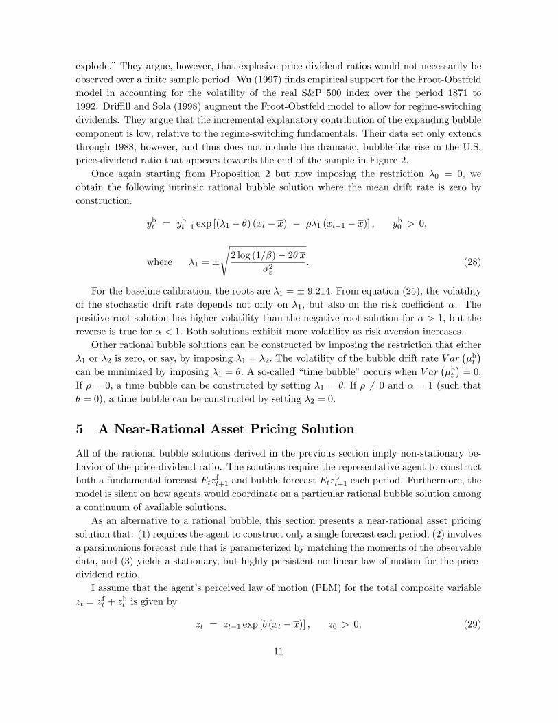
explode.�They argue, however, that explosive price-dividend ratios would not necessarily beobserved over a �nite sample period. Wu (1997) �nds empirical support for the Froot-Obstfeldmodel in accounting for the volatility of the real S&P 500 index over the period 1871 to1992. Dri¢ ll and Sola (1998) augment the Froot-Obstfeld model to allow for regime-switchingdividends. They argue that the incremental explanatory contribution of the expanding bubblecomponent is low, relative to the regime-switching fundamentals. Their data set only extendsthrough 1988, however, and thus does not include the dramatic, bubble-like rise in the U.S.price-dividend ratio that appears towards the end of the sample in Figure 2.

Once again starting from Proposition 2 but now imposing the restriction �0 = 0; weobtain the following intrinsic rational bubble solution where the mean drift rate is zero byconstruction.

ybt = ybt�1 exp [(�1 � �) (xt � x) � ��1 (xt�1 � x)] ; yb0 > 0;

where �1 = �

s2 log (1=�)� 2� x

�2": (28)

For the baseline calibration, the roots are �1 = � 9:214: From equation (25), the volatilityof the stochastic drift rate depends not only on �1; but also on the risk coe¢ cient �. Thepositive root solution has higher volatility than the negative root solution for � > 1; but thereverse is true for � < 1: Both solutions exhibit more volatility as risk aversion increases.

Other rational bubble solutions can be constructed by imposing the restriction that either�1 or �2 is zero, or say, by imposing �1 = �2: The volatility of the bubble drift rate V ar

��bt�

can be minimized by imposing �1 = �: A so-called �time bubble�occurs when V ar��bt�= 0:

If � = 0; a time bubble can be constructed by setting �1 = �: If � 6= 0 and � = 1 (such that� = 0), a time bubble can be constructed by setting �2 = 0:

5 A Near-Rational Asset Pricing Solution

All of the rational bubble solutions derived in the previous section imply non-stationary be-havior of the price-dividend ratio. The solutions require the representative agent to constructboth a fundamental forecast Etzft+1 and bubble forecast Etz

bt+1 each period. Furthermore, the

model is silent on how agents would coordinate on a particular rational bubble solution amonga continuum of available solutions.

As an alternative to a rational bubble, this section presents a near-rational asset pricingsolution that: (1) requires the agent to construct only a single forecast each period, (2) involvesa parsimonious forecast rule that is parameterized by matching the moments of the observabledata, and (3) yields a stationary, but highly persistent nonlinear law of motion for the price-dividend ratio.

I assume that the agent�s perceived law of motion (PLM) for the total composite variablezt = z

ft + z

bt is given by

zt = zt�1 exp [b (xt � x)] ; z0 > 0; (29)

11

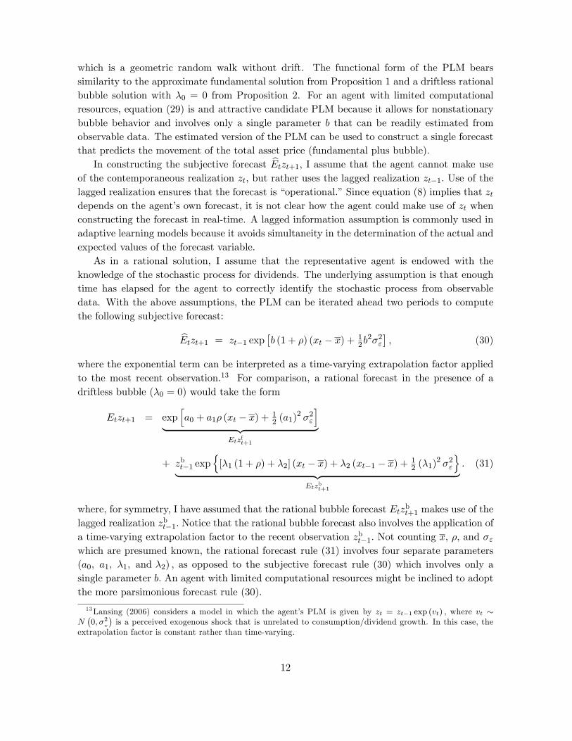
which is a geometric random walk without drift. The functional form of the PLM bearssimilarity to the approximate fundamental solution from Proposition 1 and a driftless rationalbubble solution with �0 = 0 from Proposition 2. For an agent with limited computationalresources, equation (29) is and attractive candidate PLM because it allows for nonstationarybubble behavior and involves only a single parameter b that can be readily estimated fromobservable data. The estimated version of the PLM can be used to construct a single forecastthat predicts the movement of the total asset price (fundamental plus bubble).

In constructing the subjective forecast bEtzt+1; I assume that the agent cannot make useof the contemporaneous realization zt; but rather uses the lagged realization zt�1: Use of thelagged realization ensures that the forecast is �operational.�Since equation (8) implies that ztdepends on the agent�s own forecast, it is not clear how the agent could make use of zt whenconstructing the forecast in real-time. A lagged information assumption is commonly used inadaptive learning models because it avoids simultaneity in the determination of the actual andexpected values of the forecast variable.

As in a rational solution, I assume that the representative agent is endowed with theknowledge of the stochastic process for dividends. The underlying assumption is that enoughtime has elapsed for the agent to correctly identify the stochastic process from observabledata. With the above assumptions, the PLM can be iterated ahead two periods to computethe following subjective forecast:

bEtzt+1 = zt�1 exp�b (1 + �) (xt � x) + 1

2b2�2"�; (30)

where the exponential term can be interpreted as a time-varying extrapolation factor appliedto the most recent observation.13 For comparison, a rational forecast in the presence of adriftless bubble (�0 = 0) would take the form

Etzt+1 = expha0 + a1� (xt � x) + 1

2 (a1)2 �2"

i| {z }

Etzft+1

+ zbt�1 expn[�1 (1 + �) + �2] (xt � x) + �2 (xt�1 � x) + 1

2 (�1)2 �2"

o| {z }

Etzbt+1

: (31)

where, for symmetry, I have assumed that the rational bubble forecast Etzbt+1 makes use of thelagged realization zbt�1: Notice that the rational bubble forecast also involves the application ofa time-varying extrapolation factor to the recent observation zbt�1: Not counting x; �; and �"which are presumed known, the rational forecast rule (31) involves four separate parameters(a0; a1; �1; and �2) ; as opposed to the subjective forecast rule (30) which involves only asingle parameter b: An agent with limited computational resources might be inclined to adoptthe more parsimonious forecast rule (30).

13Lansing (2006) considers a model in which the agent�s PLM is given by zt = zt�1 exp (vt) ; where vt �N�0; �2

v

�is a perceived exogenous shock that is unrelated to consumption/dividend growth. In this case, the

extrapolation factor is constant rather than time-varying.

12

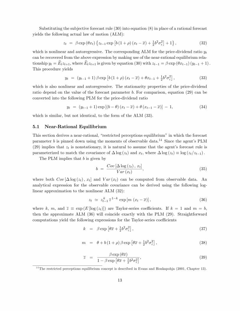
Substituting the subjective forecast rule (30) into equation (8) in place of a rational forecastyields the following actual law of motion (ALM):

zt = � exp (�xt)�zt�1 exp

�b (1 + �) (xt � x) + 1

2b2�2"�+ 1; (32)

which is nonlinear and autoregressive. The corresponding ALM for the price-dividend ratio ytcan be recovered from the above expression by making use of the near-rational equilibrium rela-tionship yt = bEtzt+1; where bEtzt+1 is given by equation (30) with zt�1 = � exp (�xt�1) (yt�1 + 1) :This procedure yields

yt = (yt�1 + 1)� exp�b (1 + �) (xt � x) + �xt�1 + 1

2b2�2"�; (33)

which is also nonlinear and autoregressive. The stationarity properties of the price-dividendratio depend on the value of the forecast parameter b: For comparison, equation (29) can beconverted into the following PLM for the price-dividend ratio

yt = (yt�1 + 1) exp [(b� �) (xt � x) + � (xt�1 � x)] � 1; (34)

which is similar, but not identical, to the form of the ALM (33).

5.1 Near-Rational Equilibrium

This section derives a near-rational, �restricted perceptions equilibrium�in which the forecastparameter b is pinned down using the moments of observable data.14 Since the agent�s PLM(29) implies that zt is nonstationary, it is natural to assume that the agent�s forecast rule isparameterized to match the covariance of � log (zt) and xt, where � log (zt) � log (zt=zt�1) :

The PLM implies that b is given by

b =Cov [� log (zt) ; xt]

V ar (xt); (35)

where both Cov [� log (zt) ; xt] and V ar (xt) can be computed from observable data. Ananalytical expression for the observable covariance can be derived using the following log-linear approximation to the nonlinear ALM (32):

zt ' z kt�1 z1�k exp [m (xt � x)] ; (36)

where k; m; and z � exp (E [log (zt)]) are Taylor-series coe¢ cients. If k = 1 and m = b;

then the approximate ALM (36) will coincide exactly with the PLM (29). Straightforwardcomputations yield the following expressions for the Taylor-series coe¢ cients

k = � exp��x+ 1

2b2�2"�; (37)

m = � + b (1 + �)� exp��x+ 1

2b2�2"�; (38)

z =� exp (�x)

1� � exp��x+ 1

2b2�2"� ; (39)

14The restricted perceptions equilibrium concept is described in Evans and Honkapohja (2001, Chapter 13).

13

which all depend in a nonlinear way on the subjective forecast parameter b: The approximatelaw of motion of � log (zt) can be computed directly from equation (36), which in turn yieldsthe following expression for the relevant covariance

Cov [� log (zt) ; xt] =

�(1� �)m1� �k

�V ar (xt) ; (40)

which is nonlinear in b via the expressions for k and m: Details are contained in the appendix.Equations (35) and (40) can be combined to form the following de�nition of equilibrium.

De�nition 1. A near-rational �restricted perceptions equilibrium� is de�ned as a perceivedlaw of motion (29), an approximate actual law of motion (36), and a subjective forecast ruleparameter b; such that the equilibrium value b is given by the �xed point of the nonlinear map

b = T (b) � (1� �) m (b)1� � k (b) ;

where k (b) and m (b) are parameters of the approximate actual law of motion that depend onb, as given by equations (37) and (38), provided that 0 � k (b) � 1:

In equilibrium, we require 0 � k (b) � 1 so that � log (zt) remains stationary, therebyallowing Cov [� log (zt) ; xt] to be computed from observable data. If 0 � k (b) < 1; thenlog (zt) and log (yt) are stationary.

The approximate ALM (36) can be used to derive the following analytical expressions forthe unconditional moments of the asset pricing variables

E [log (yt)] = log

�k (b)

1� k (b)

�; 0 � k (b) < 1; (41)

E [log (Rt+1)] = � log (�) + �x � 12b2�2", (42)

where k (b) is given by equation (37). Notice that the expression for E [log (Rt+1)] has thesame form as the fundamental mean return E

�log�Rft+1

��given by equation (18), except that

(a1)2 is replaced here by b2: At the baseline calibration, we have a1 = �0:457: As shown in the

next section, the near-rational equilibrium yields b = �3:695; which causes the near-rationalmean return to be below that of the fundamental mean return. This result can be tracedto a small degree of excess optimism in the near-rational forecast rule. Excess optimism hasan e¤ect on the mean return that is similar to increasing patience about future payo¤s viaa higher value for the discount factor �: The appendix outlines the derivation of analyticalexpressions for the unconditional variances V ar [log (yt)] and V ar [log (Rt+1)] :

5.2 Numerical Solution for the Equilibrium

The complexity of the nonlinear map b = T (b) necessitates a numerical solution for theequilibrium. Using the baseline calibration, panel (a) of Figure 3 plots plots T (b) over the range�25 � b � 20: There are three �xed points. At the middle �xed point, we have b = �3:695:From panel (b), we see that only the middle �xed point yields a stationary equilibrium such

14

that 0 � k (b) < 1. When b = �3:695; the autoregressive root in the approximate ALM (36)is k = 0:956: The corresponding response coe¢ cient on (xt � x) in the ALM is m = �3:680:Recall that when k = 1 and m = b; the approximate ALM (36) coincides exactly with thePLM (29). At the middle �xed point, we have k ' 1 and m ' b; such that the equilibriumcan be described as �near-rational.�

Making use of the approximate ALM (36) and the subjective forecast rule (30), the per-centage forecast error observed by the agent is given by

errt+1 = log

zt+1bEtzt+1

!;

= log

(z kt z

1�k exp [m (xt+1 � x)]zt�1 exp

�b (1 + �) (xt � x) + 1

2b2�2"�) ; (43)

where k and m are given by equations (37) and (38). Recalling that z = exp (E [log (zt)]) ;

the above equation implies E (errt+1) = �b2�2"=2: At the equilibrium value b = �3:695; with�" = 0:0354, we have E (errt+1) = �0:009: In contrast, the approximate fundamental solutionimplies E

�errft+1

�= �0:0001 for the same calibration.

Equation (43) can be used to derive an analytical expression for the autocorrelation ofpercentage forecast errors Corr (errt+1; errt) ; as outlined in the appendix. The value ofCorr (errt+1; errt) is plotted in panel (c) of Figure 3. At the equilibrium value b = �3:695;the correlation coe¢ cient is 0:02: The near-zero autocorrelation of the forecast errors makesit di¢ cult for the agent to detect a misspeci�cation of the subjective forecast rule (30). Panel(d) of Figure 3 plots the root mean squared percentage forecast error (RMSPE), de�ned as�E�err2t+1

��0:5 At the equilibrium value, we have RMSPE = 13:5 %: Since RMSPE couldbe reduced by shrinking the magnitude of the subjective forecast parameter b; the agent canbe viewed as exhibiting overreaction to the fundamental term (xt � x) :15 The fundamentalsolution implies RMSPE f = 1:62 % for the same calibration.

5.3 Real-Time Learning

Figure 4 illustrates the convergence properties of the near-rational equilibrium under real-timelearning. Recall that the �xed point of the nonlinear map b = T (b) is computed using theapproximate population covariance statistic Cov [� log (zt) ; xt] ; as given by equation (40).This statistic presumes a �xed forecast parameter b: However, in a real-time learning environ-ment where the forecast parameter evolves over time, the agent will only have knowledge of asample covariance which, in turn, is in�uenced by the trajectory of the forecast parameter.

The real-time learning algorithm makes use of the nonlinear ALM for zt; equation (32).The forecast parameter bt�1 that is used in computing zt is estimated each period (startingat t = 5) using equation (35) with an expanding window of data that runs through timet � 1: The stochastic process for dividends (3) is presumed known by the agent. Figure 415Lansing (2009) considers the welfare cost of speculative overreaction in a production economy with endoge-

nous long-run consumption growth.

15

plots twelve learning simulations of length 5000 periods using a starting value for the forecastparameter that is set �5 above or below the theoretical equilibrium value for the �rst �veperiods. The starting value z0 is computed from equation (39) with b = b0: The end-of-simulation values are clustered in the range where the (approximate) theoretical map T (b)lies very close to the 45-degree line. Given the shape of the map and the nonlinear form of theALM (32), a small amount of sampling variation in the covariance statistic can a¤ect the speedof convergence and the end-of-simulation value. For the twelve learning simulations shown, theaverage end-of-simulation value is �3:752; which is close to the theoretical equilibrium valueof b = �3:695 computed using the approximate ALM (36). The simulations demonstrate thatthe near-rational equilibrium is learnable.

The technical condition that must be satis�ed for learnability (or �E-stability�) is T 0 (b) <1:16 In the special case of iid consumption growth (� = 0) and logarithmic utility (� = 0) ; theexpression for T (b) reduces to

T (b) = b� exp�b2�2"=2

�; (44)

which has three �xed points given by b = f 0; �p2 log (1=�) =�2" g: It is easy to check that

the middle �xed point b = 0 satis�es the learnability condition T 0 (b) = � < 1; while theother two solutions yield T 0 (b) = 1 + b2�2" > 1 and hence are not stable under learning. Bycontinuity, these results extend to parameter combinations (�; �) that are su¢ ciently closeto (0; 0) and for starting values that lie in the basin of attraction of the middle �xed point.For the baseline calibration with (�; �) = (�0:1; �0:5) ; the properties of the near-rationalequilibrium are qualitatively similar to the special case of (�; �) = (0; 0) :17

Numerical experiments with the model show that as consumption growth becomes morepersistent (� increases) or as the agent become more risk averse (� increases), satisfying thelearnability condition T 0 (b) < 1 may require the discount factor � to remain below a thresholdvalue. It is worth noting, however, that even when a parameter combination does not satisfyT 0 (b) < 1; it would still be possible for the agent to estimate a value of b using a rolling windowof past data. In this case, the learning algorithm would never converge to a �xed point, butrather, the estimated value of b would drift over time, acting as an additional source of excessvolatility.18

6 Model Simulations

Table 1 presents unconditional moments of asset pricing variables computed from a long-runsimulation of the model. The table also reports the corresponding statistics from U.S. dataover the period 1871 to 2008.19 The fundamental solution is simulated using the expressions

16For details, see Evans and Honkapohja (2001, p. 39).17 I thank an anonymous referee for providing this insight.18The learning algorithm may need to be modi�ed in this case to include a �projection facility,�which sets

bt = bt�1 if the estimation procedure delivers a result that falls outside the agent�s preconceived range ofeconomically reasonable values.19The price-dividend ratio in year t is de�ned as the value of the S&P 500 stock index at the beginning of

year t+ 1; divided by the accumulated dividend over year t:

16

in Proposition 1. Equations (26) and (28) are used to simulate the rational bubble solutions,which are superimposed on top of the fundamental solution.20 For the rational bubble so-lutions, the initial level of the bubble component yb0 is set equal to 1 % of the steady-statefundamental price-dividend ratio. For the fundamental and near-rational solutions, the initialcondition is the corresponding steady-state price-dividend ratio.

The top section of Table 1 shows that the near-rational solution does an excellent job ofmatching the unconditional moments of the U.S. price-dividend ratio. The calibrated valuesof � and � were chosen so that the near-rational solution comes close to matching the meanand volatility of the U.S. price-dividend ratio.21 But the near-rational solution also does agood job of matching the higher moments. In particular, the U.S. price-dividend ratio exhibitspositive skewness, excess kurtosis, and strong positive serial correlation. Positive skewness andexcess kurtosis suggest the presence of nonlinearities in the data. The near-rational solutionis able to capture these features due to the non-linear form of the ALM for yt; equation (33).In contrast, the fundamental solution delivers low volatility, near-zero skewness, no excesskurtosis, and weak negative serial correlation which is inherited directly from the consumptiongrowth process with � = �0:1. The rational bubble solutions imply that the price-dividendratio is non-stationary, so the corresponding moments do not exist.

The middle section of Table 1 compares unconditional moments for the drift rate of theprice-dividend ratio� a stationary variable for all model solutions. The mean drift rate inU.S. data is 0.004 versus a drift rate of 0.05 for the Froot-Obstfeld solution.22 The �DriftlessBubble 2�solution and the near-rational solution both produce a reasonably good match withthe moments in the data.

The last section of Table 1 compares unconditional moments for the equity return. Relativeto the fundamental solution, the mean return for the near-rational solution is slightly lower(6.96 % versus 7.68 %), whereas the volatility of returns is higher (9.08 % versus 4.04 %). Thereturns generated by the near-rational solution exhibit only a small amount of positive serialcorrelation, albeit slightly stronger than in U.S. data.

Figure 5 plots simulated data for the di¤erent solutions of the model. The left-side panelsshow the price dividend ratio yt = yft + y

bt ; while the right-side panels show the net equity

return Rt � 1: The explosive price-dividend ratio in the Froot-Obstfeld solution with �1 > 0can be seen in panel (a), which in the only panel to employ a logarithmic scale. In panel (b),the equity return generated by the Froot-Obstfeld solution remains stationary and exhibitstime-varying volatility. In panels (c) and (e), the two driftless rational bubble solutions exhibitwhat can be viewed as stylized bubbles and crashes, where the price dividend ratio undergoesirregularly-spaced episodes of rapid expansions and contractions. Return volatility increases

20�Driftless Bubble 1�refers to the solution shown in equation (28) with �1 > 0; while �Driftless Bubble 2�refers to the solution with �1 < 0:21 If the model is recalibrated with � = 0 rather than � = �0:1; then the ability to match both of these

moments deteriorates because either � or � must be adjusted downward to ensure that the learnability conditionis satis�ed, as described in section 5.3.22 In Table 1, the mean drift rate in U.S. data is estimated by taking the average of annual log changes. In

Figure 2, the mean drift rate is estimated by �tting an exponential time trend through the data. The latterprocedure yields a larger estimated drift rate.

17

dramatically during these episodes, as shown in panels (d) and (f).

Table 1. Unconditional Moments

Model Simulations

StatisticU.S. Data1871 �2008

Funda-mental

Froot-Obstfeld

DriftlessBubble 1

DriftlessBubble 2

Near-Rational

yt = pt=dt � � �Mean 26.6 18.4 � � � 27.1

Std. Dev. 13.8 0.03 � � � 13.9Skew. 2.20 �0:02 � � � 2.34Kurt. 8.21 3.00 � � � 11.7

Corr. Lag 1 0.93 �0:11 � � � 0.97

log (yt=yt�1)Mean 0.004 0.000 0.050 0.000 0.003 0.000

Std. Dev. 0.206 0.002 0.082 0.042 0.269 0.119Skew. �0:12 0.03 �0:03 0.59 0.04 0.03Kurt. 3.19 2.99 3.00 125.2 3.89 3.00

Corr. Lag 1 �0:07 �0:55 �0:03 �0:10 0.00 0.02

Rt � 1Mean 7.84 % 7.68 % 8.06 % 7.66 % 6.59 % 6.96 %

Std. Dev 17.8 % 4.04 % 12.7 % 6.84 % 25.9 % 9.08 %Skew. �0:05 0.09 0.33 3.69 0.95 0.28Kurt. 2.87 3.02 3.21 92.7 5.40 3.13

Corr. Lag 1 0.04 �0:15 �0:06 �0:12 0.00 0.14

Note: Model statistics are based on a 12,000 period simulation after dropping 500 periods.Parameter values: x = 0:0206; �" = 0:0354; � = �0:1; � = 1:5; and � = 0:958:

Table 2. 20-Year Rolling Volatility of Returns

Model Simulations

Std. Dev.U.S. Data1871 �2008

Funda-mental

Froot-Obstfeld

DriftlessBubble 1

DriftlessBubble 2

Near-Rational

Min 20-Yr 12.5 % 1.77 % 3.06 % 1.77 % 0.93 % 4.41 %Max 20-Yr 27.9 % 7.07 % 23.4 % 65.5 % 48.7 % 13.8 %Full Sample. 17.8 % 4.04 % 12.7 % 6.84 % 25.9 % 9.08 %

Notes: Model statistics are based on a 12,000 period simulation after dropping 500 periods.Parameter values: x = 0:0206; �" = 0:0354; � = �0:1; � = 1:5; and � = 0:958:

18

In panel (g), the near-rational price-dividend ratio exhibits pronounced low-frequencyswings that are driven by random shocks impinging upon the highly-persistent, nonlinearALM (33). The near-rational solution can also generate periods where the price-dividendratio dips below the fundamental value. In contrast, a rational bubble solution requires theprice-dividend ratio to always remain above the fundamental.23 The timing of expanding andcontracting bubble episodes in panel (g) is somewhat similar to that generated by the driftlessrational bubble solution with �1 < 0 plotted in panel (e). Both solutions exhibit a negativeresponse coe¢ cient on the fundamental term (xt � x) in the corresponding law of motion.

The nonlinear nature of the exact ALM (33) gives rise to time-varying return volatility,as shown in panel (h). Table 2 provides a quantitative comparison of the return volatilities inU.S. data and the various model solutions. From 1871 to 2008, the 20�year rolling standarddeviation of U.S. returns varies from a minimum of 12.5% to a maximum of 27.9%. TheFroot-Obstfeld solution provides the best match with the data, followed by the near-rationalsolution.

Table 3 provides a quantitative comparison of forecast errors between the fundamental andnear-rational solutions. As noted earlier, the fundamental solution delivers a lower RMSPE.However, the near-rational forecast errors are close to white noise at all lags� giving no dis-cernible indication to the agent that the subjective forecast rule (30) is misspeci�ed.

Table 3: Comparison of Percentage Forecast Errors

Model SimulationsStatistic Fundamental Near-RationalE (errt+1) 0:000 �0:010�E�err2t+1

��0:50:016 0:136

Corr (errt+1; errt) �0:01 0:02Corr (errt+1; errt�1) �0:01 �0:02Corr (errt+1; errt�2) �0:01 �0:01Notes: Model statistics are based on a 12,000 period simulation after dropping 500 periods.Parameter values: x = 0:0206; �" = 0:0354; � = �0:1; � = 1:5; and � = 0:958:

6.1 Empirical Tests

To provide a more direct empirical assessment of the near-rational solution, I regress thePLM (34) in �rst-di¤erence form on U.S. data for the price-dividend ratio and per capitaconsumption growth over the period 1891 to 2004. The regression implements a procedurefor estimating the parameter b; analogous to the agent�s use of the covariance expression (35)in the model. For the regression, I impose � = 1:5 and x = 0:0206:24 The regression yieldsb = �1:56 (s.e. = 0:50); which is in the ballpark of the theoretical value of b = �3:695:23Weil (1990) notes that a positive rational bubble can cause the equilibrium asset price to dip below the ex

ante fundamental value if there is su¢ cient feedback from the bubble to either dividends or the discount rate.24With these parameter restrictions, the regression equation becomes �log (yt + 1) =

(b+ 0:5) (xt � 0:0206) � 0:5 (xt�1 � 0:0206) ; where yt is the U.S. price-dividend ratio and xt is U.S.per capita consumption growth.

19

More generally, there is a vast literature on econometric tests for the presence of bubbles.Some recent studies are closely related to the results presented here. Bohl and Siklos (2004)and Coakley and Fuertes (2006) �t nonlinear time series models to U.S. stock market valua-tion ratios over the period 1871 to 2001. Both studies �nd evidence that valuation ratios driftupwards into bubble territory during bull markets, but these persistent departures from fun-damentals are eventually eliminated via downward adjustments during bear markets. Recentempirical tests for nonstationarity of the U.S. price-dividend ratio are inconclusive. Engsted(2006) �nds support for a nonstationary rational bubble in U.S. data. In contrast, a study byKoustas and Serletis (2005) rejects the rational bubble hypothesis in favor of mean-revertingbehavior for the U.S. price-dividend ratio. The near-rational solution derived here predictsmean-reverting behavior for the price-dividend ratio.

In reviewing the literature on empirical tests for the presence of bubbles, Gürkaynak (2007)concludes that a su¢ ciently-rich fundamental model of asset prices can often �t the dataequally as well as any bubble model. Cochrane (2009) argues that the concept of a bub-ble driven by irrational expectations of the future is observationally equivalent to a situationwhere the risk premium required by rational agents is temporarily low.25 But actually thesetwo scenarios can be distinguished by examining agents�expectations about future returns.Irrationally exuberant agents would forecast high future returns following a sustained pricerun-up, whereas rational agents with temporarily low risk premiums would forecast low futurereturns. Evidence from investor survey data seems to support the former scenario. Vissing-Jorgenson (2004) �nds evidence of extrapolative expectations among investors; those who haveexperienced high portfolio returns in the past tend to expect higher returns in the future. Am-romin and Sharpe (2009) �nd that household investors expect higher future returns duringperiods when macroeconomic conditions are expected to improve� a result which they con-clude �is inconsistent with the view that stock market returns should compensate [rational]investors for exposure to macroeconomic risks.�

7 Concluding Remarks

Theories involving departures from fully-rational behavior have long played a role in e¤ortsto account for the behavior of asset prices. Keynes (1936, p. 156) likened the stock marketto a �beauty contest�where participants devoted their e¤orts not to judging the underlyingconcept of beauty, but instead to �anticipating what average opinion expects the averageopinion to be.�

There are many examples in history of asset prices exhibiting sustained run-ups that aredi¢ cult to justify on the basis of economic fundamentals. The typical transitory nature ofthese run-ups should perhaps be viewed as a long-run victory for fundamental asset pricingtheory. Still, it remains a challenge for fundamental theory to explain the ever-present volatil-ity of asset prices within a framework of e¢ cient capital markets. Rational bubbles are anattractive modeling device because the framework allows asset prices to exceed fundamentals

25Speci�cally, he remarks (p. 2) that �Crying �bubble�is empty unless you have an operational procedure fordistinguishing them from rationally low risk premiums...�

20

while imposing a no-arbitrage condition over short time horizons. In a rational bubble solu-tion, an asset is valued not for its cash �ows, but rather for its potential to deliver capitalgain� a feature that seems to �t the prevailing psychology during historical bubble episodes.

This paper demonstrated the existence of a continuum of intrinsic rational bubble solutionsthat satisfy a period-by-period no-arbitrage condition. When the mean drift rate of the bubbleis zero by construction, the short-term prospects for capital gain derive solely from the highvolatility of the bubble component. A driftless rational bubble exhibits irregularly-spacedexpansions and collapses that are wholly endogenous.

Strictly speaking, rational bubbles are not fully rational because the transversality con-dition is not satis�ed. In a world where agents�computational resources are limited, furthermovements away from full rationality would seem plausible. The near-rational asset pricingsolution developed here is based on a parsimonious and versatile forecast rule: a geometricrandom walk without drift. Innovations to the geometric random walk are linked to consump-tion/dividend growth. When the agent�s forecast rule is parameterized to match the momentsof observable data, the resulting forecast errors are close to white noise. The near-rationalsolution does a good job of matching many quantitative features of U.S. stock market dataand allows the equity price to occasionally dip below the fundamental price.

21

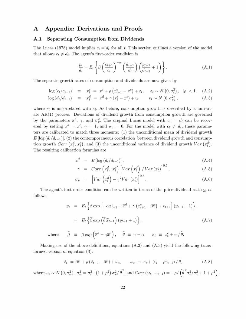
A Appendix: Derivations and Proofs

A.1 Separating Consumption from Dividends

The Lucas (1978) model implies ct = dt for all t: This section outlines a version of the modelthat allows ct 6= dt: The agent�s �rst-order condition is

ptdt= Et

(�

�ct+1ct

����dt+1dt

��pt+1dt+1

+ 1

�): (A.1)

The separate growth rates of consumption and dividends are now given by

log (ct=ct�1) � xct = xc + ��xct�1 � xc

�+ "t; "t � N

�0; �2"

�; j�j < 1; (A.2)

log (dt=dt�1) � xdt = xd + (xct � xc) + vt vt � N�0; �2v

�; (A.3)

where vt is uncorrelated with "t: As before, consumption growth is described by a univari-ate AR(1) process. Deviations of dividend growth from consumption growth are governedby the parameters xd; ; and �2v: The original Lucas model with ct = dt can be recov-ered by setting xd = xc; = 1; and �v = 0: For the model with ct 6= dt; these parame-ters are calibrated to match three moments: (1) the unconditional mean of dividend growthE [log (dt=dt�1)], (2) the contemporaneous correlation between dividend growth and consump-tion growth Corr

�xdt ; x

ct

�, and (3) the unconditional variance of dividend growth V ar

�xdt�.

The resulting calibration formulas are

xd = E [log (dt=dt�1)] ; (A.4)

= Corr�xdt ; x

ct

� hV ar

�xdt

�= V ar (xct)

i0:5; (A.5)

�v =hV ar

�xdt

�� 2V ar (xct)

i0:5: (A.6)

The agent�s �rst-order condition can be written in terms of the price-dividend ratio yt asfollows:

yt = Et

n� exp

h��xct+1 + xd +

�xct+1 � xc

�+ vt+1

i(yt+1 + 1)

o;

= Et

ne� exp�e� ext+1� (yt+1 + 1)o ; (A.7)

where e� � � exp�xd � xc

�; e� � � �; ext � xct + vt=

e�:Making use of the above de�nitions, equations (A.2) and (A.3) yield the following trans-

formed version of equation (3):

ext = xc + � (ext�1 � xc) + !t; !t � "t + (vt � �vt�1) =e�; (A.8)

where !t � N�0; �2!

�; �2! = �

2"+�1 + �2

��2v=

e� 2, and Corr (!t; !t�1) = ��=�e� 2�2"=�2v + 1 + �2� :22

Finally, we de�ne ezt � e� exp�e� ext� (yt + 1) to obtain the following transformed version ofequation (8): ezt = e� exp�e� ext� [Etezt+1 + 1] : (A.9)

Thus, by an appropriate change of variables, equations (A.8) and (A.9) retain the samebasic forms as equations (3) and (8), with the exception that the innovation !t is not iid, butinstead exhibits serial correlation. However, for small values of �; we can make the simplifyingassumption that Corr (!t; !t�1) ' 0: With this assumption, all of the paper�s theoreticalresults will go through when expressed in terms of the transformed variables.

A.2 Proof of Proposition 1: Approximate Fundamental Solution

Iterating ahead the conjectured law of motion for zft and taking the conditional expectationyields

Etzft+1 = exp

ha0 + �a1 (xt � x) + 1

2 (a1)2 �2"

i: (A.10)

Substituting the above expression into the �rst order condition (8) and then taking logarithmsyields

log�zft

�= F (xt) = log (�) + �xt

+ lognexp

ha0 + �a1 (xt � x) + 1

2 (a1)2 �2"

i+ 1o;

' a0 + a1 (xt � x) ; (A.11)

where a0 � E�log�zft��and a1 are Taylor-series coe¢ cients which are are given by

F (x) = a0 = log (�) + �x+ lognexp

ha0 +

12 (a1)

2 �2"

i+ 1o

(A.12)

F0(x) = a1 = � +

�a1 expha0 +

12 (a1)

2 �2"

iexp

ha0 +

12 (a1)

2 �2"

i+ 1

: (A.13)

Solving equation (A.12) for a0 yields

a0 = log

8<: � exp (�x)

1� � exph�x+ 1

2 (a1)2 �2"

i9=; ; (A.14)

which can be substituted into equation (A.13) to yield the following nonlinear equation thatdetermines a1:

a1 = � + �a1� exph�x+ 1

2 (a1)2 �2"

i: (A.15)

Solving equation (A.15) for a1 yields the nonlinear equation shown in Proposition 1. There

are two solutions, but only one solution satis�es the condition � exph�x+ 1

2 (a1)2 �2"

i< 1 such

that exp (a0) = exp�E log

�zft��> 0: �

23

A.3 Asset Pricing Moments: Fundamental Solution

This section brie�y outlines the derivation of equations (16) through (19).Equation (16) follows directly from equation (15) by taking the unconditional expectation

of log�yft�: We have

log�yft

�� E

hlog�yft

�i= a1�1 (xt � x) ; (A.16)

which implies V ar�log�yft��= (a1)

2 �2V ar (xt) ; as given by equation (17).The fundamental equity return can be written as

Rft+1 =

yft+1 + 1

yft

!exp (xt+1) ;

=

zft+1

�Etzft+1

!exp (�xt+1) ; (A.17)

where I have eliminated yft using the equilibrium relationship yft = Etzft+1 and eliminated y

ft+1

using the de�nitional relationship yft+1 + 1 = ��1 exp (��xt+1) zft+1: Substituting in zft+1 =exp [a0 + a1 (xt � x)] from Proposition 1 and Etzft+1 from equation (15) and then taking theunconditional expectation of log

�Rft+1

�yields equation (18). We have

log�Rft+1

�� E

hlog�Rft+1

�i= � (xt+1 � x) + a1"t+1; (A.18)

which in turns implies

V arhlog�Rft+1

�i= �2V ar (xt) + (a1)

2 �2" + 2�a1Cov (xt; "t) : (A.19)

Substituting for V ar (xt) and Cov (xt; "t) in the above expression yields equation (19).

A.4 Proof of Proposition 2: Continuum of Intrinsic Rational Bubbles

First consider the case where the agent can make use of the contemporaneous realization zbtwhen forming the rational expectation Etzbt+1: Iterating ahead the conjectured law of motionfor zbt by one period and then taking the conditional expectation yields

Etzbt+1 = z

bt exp

h�0 + (��1 + �2) (xt � x) + 1

2 (�1)2 �2"

i: (A.20)

Substituting the above expression into the no-arbitrage condition (21) and then taking loga-rithms yields

0 = log (�) + �xt + �0 + (��1 + �2) (xt � x) + 12 (�1)

2 �2"; (A.21)

where log�zbt�has been cancelled from both sides. For equation (A.21) to hold, the constant

terms and the coe¢ cients on xt must separately sum to zero. Equilibrium therefore requires

12 (�1)

2 �2" � (��1 + �2)| {z }� �

x + log (�) + �0 = 0; (A.22)

� + ��1 + �2 = 0; (A.23)

24

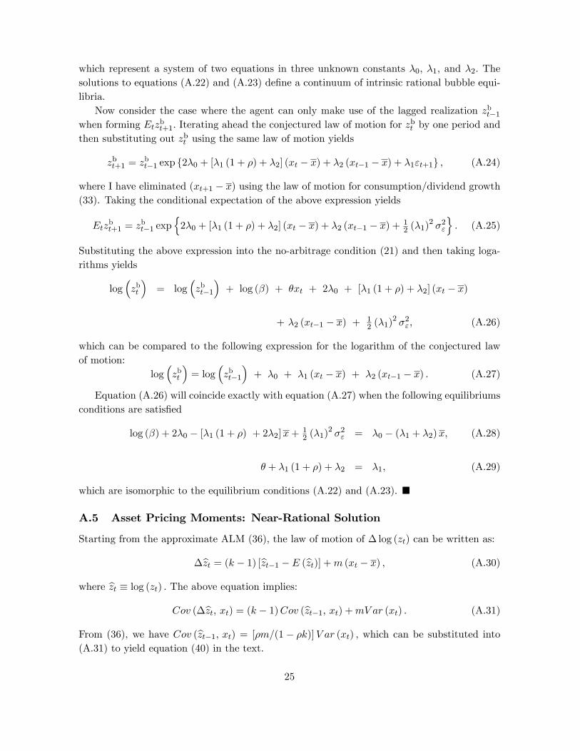
which represent a system of two equations in three unknown constants �0; �1; and �2: Thesolutions to equations (A.22) and (A.23) de�ne a continuum of intrinsic rational bubble equi-libria.

Now consider the case where the agent can only make use of the lagged realization zbt�1when forming Etzbt+1: Iterating ahead the conjectured law of motion for z

bt by one period and

then substituting out zbt using the same law of motion yields

zbt+1 = zbt�1 exp f2�0 + [�1 (1 + �) + �2] (xt � x) + �2 (xt�1 � x) + �1"t+1g ; (A.24)

where I have eliminated (xt+1 � x) using the law of motion for consumption/dividend growth(33). Taking the conditional expectation of the above expression yields

Etzbt+1 = z

bt�1 exp

n2�0 + [�1 (1 + �) + �2] (xt � x) + �2 (xt�1 � x) + 1

2 (�1)2 �2"

o: (A.25)

Substituting the above expression into the no-arbitrage condition (21) and then taking loga-rithms yields

log�zbt

�= log

�zbt�1

�+ log (�) + �xt + 2�0 + [�1 (1 + �) + �2] (xt � x)

+ �2 (xt�1 � x) + 12 (�1)

2 �2"; (A.26)

which can be compared to the following expression for the logarithm of the conjectured lawof motion:

log�zbt

�= log

�zbt�1

�+ �0 + �1 (xt � x) + �2 (xt�1 � x) : (A.27)

Equation (A.26) will coincide exactly with equation (A.27) when the following equilibriumsconditions are satis�ed

log (�) + 2�0 � [�1 (1 + �) + 2�2]x+ 12 (�1)

2 �2" = �0 � (�1 + �2)x; (A.28)

� + �1 (1 + �) + �2 = �1; (A.29)

which are isomorphic to the equilibrium conditions (A.22) and (A.23). �

A.5 Asset Pricing Moments: Near-Rational Solution

Starting from the approximate ALM (36), the law of motion of � log (zt) can be written as:

�bzt = (k � 1) [bzt�1 � E (bzt)] +m (xt � x) ; (A.30)

where bzt � log (zt) : The above equation implies:Cov (�bzt; xt) = (k � 1)Cov (bzt�1; xt) +mV ar (xt) : (A.31)

From (36), we have Cov (bzt�1; xt) = [�m=(1� �k)]V ar (xt) ; which can be substituted into(A.31) to yield equation (40) in the text.

25

The nonlinear ALM for the price-dividend ratio, equation (33), can be rewritten as follows:

yt = (yt�1 + 1)� exp�b (1 + �) (xt � x) + �xt�1 + 1

2b2�2"�;

= (yt�1 + 1) k exp

��m� �k

�(xt � x) + � (xt�1 � x)

�; (A.32)

where I have eliminated b and b2 using the expressions for the Taylor series coe¢ cients k andm; as given by equations (37) and (38). Taking logarithms of the above expression yields

byt = log [exp (byt�1) + 1] + log (k) + �m� �k

�(xt � x) + � (xt�1 � x) ;

' n0 + n1 [byt�1 � E (byt)] + �m� �k

�(xt � x) + � (xt�1 � x) ; (A.33)

where byt � log (yt) ; and n0 and n1 are Taylor series coe¢ cients. Straightforward computationsyield n0 = log [k= (1� k)] and n1 = k: The unconditional expectation of the above expressionyields E (byt) = n0; as given by equation (41).

Using equation (A.33), the unconditional variance can be computed as follows:

V ar (byt) = En[byt � E (byt)]2o ;

=

�1

1� k2

�"�m� �k

�2+ �2 + 2

�m� �k

���

#V ar (xt) ;

+

�2 (m� �) �+ 2�k

1� k2

�Cov (byt; xt) ; (A.34)

where Cov (byt; xt) can also be computed from equation (A.33).The equity return is given by

Rt+1 =

zt+1

� bEtzt+1!exp (�xt+1)

=z kt z

1�k exp [m (xt+1 � x) + �xt+1]�zt�1 exp

�b (1 + �) (xt � x) + 1

2b2�2"� ; (A.35)

where I have substituted in the approximate ALM (36) and the subjective expectation (30).Taking the unconditional expectation of bRt+1 � log (Rt+1) yields equation (42). From (A.35),we have

bRt+1 � E � bRt+1� = k [bzt � E (bzt)]| {z }k2[bzt�1�E(bzt)]+ km(xt�x)

� [bzt�1 � E (bzt)]+ (m+ �) (xt+1 � x) � b (1 + �) (xt � x) ; (A.36)

26

which can be used to compute an analytical expression for V ar� bRt+1� :

From equation (43), the law of motion for the percentage forecast error is given by

errt+1 � E (errt+1) = ��1� k2

�[bzt�1 � E (bzt)]

+ [km+m�� b (1 + �)] (xt � x) +m"t+1; (A.37)

where I have eliminated [bzt � E (bzt)] using the approximate ALM (36). Equation (A.37)is used to compute Corr (errt+1; errt) = Cov (errt+1; errt) =V ar (errt+1) and RMSPE =�E�err2t+1

��0:5 which are plotted in Figure 3.

27

Adam, K., A. Marcet, and Nicolini, J.P. (2008). �Stock market volatility and learning�, Euro-pean Central Bank, working paper 862 (February).Abel, A.B. (2002). �An exploration of the e¤ects of pessimism and doubt on asset returns�,Journal of Economic Dynamics and Control, vol. 26 (July), pp. 1075-1092.Amromin, G. and Sharpe, S.A. (2009). �Expectations of risk and return among householdinvestors: Are their Sharpe ratios countercycilical?,�Working paper (February).Abreu, D. and Brunnermeier, M.K. (2003). �Bubbles and crashes�, Econometrica, vol. 71(January), pp. 173-204.Barberis, N., A. Shleifer, and Vishny, R.W. (1998). �A model of investor sentiment�, Journalof Financial Economics, vol. 49 (September), pp. 307-343.Barsky, R.B. and De Long, J.B. (1993). �Why does the stock market �uctuate?�, QuarterlyJournal of Economics, vol. 107 (May), pp. 291-311.Bidarkota, P.V. and Dupoyet, B.V., (2007). �Intrinsic bubbles and fat tails: A note�, Macro-economic Dynamics, vol. 11 (June), pp. 405-422.Bohl, M.T. and Siklos, P.L. (2004). �The present value model of U.S. stock prices redux: Anew testing strategy and some evidence�, Quarterly Review of Economics and Finance, vol.44 (May), pp. 208-223.Blanchard, O.J. (1979). �Speculative bubbles, crashes, and rational expectations�, EconomicsLetters, vol. 3 (November), pp. 387-389.Blanchard, O.J. and Watson, M.W. (1982). �Bubbles, rational expectations and �nancialmarkets�, in (P. Wachtel, ed.), Crises in the Economic and Financial Structure, pp. 295-315.Lexington MA: Lexington Books.Branch, W.A. and Evans, G.W. (forthcoming). �Asset return dynamics and learning�, Reviewof Financial Studies.Brock, W.A. and Hommes, C.H. (1998). �Heterogenous beliefs and routes to chaos in a simpleasset pricing model�, Journal of Economic Dynamics and Control, vol. 22 (August), pp. 1235-1274.Bullard, J., Evans, G., and Honkapohja, S. (forthcoming). �A model of near-rational exuber-ance�, Macroeconomic Dynamics.Branch, W.A. and Evans, G.W. (forthcoming). �Asset return dynamics and learning�, Reviewof Financial Studies.Burnside, C. (1998). �Solving asset pricing models with Gaussian shocks�, Journal of EconomicDynamics and Control, vol. 22 (March), pp. 329-340.Calin, O.L., Chen, Y., Cosimano, T.F., and Himonas, A.A. (2005). �Solving asset pricingmodels when the price-dividend ratio function is analytic�, Econometrica, vol. 73 (May), pp.961-982.Cecchetti, S.G., Lam, P.-S. and Mark, N.C. (2000). �Asset pricing with distorted beliefs: Areequity returns too good to be true?�, American Economic Review, vol. 90 (September), pp.787-805.Coakley, J. and Fuertes, A. (2006). �Valuation ratios and price deviations from fundamentals�,Journal of Banking and Finance, vol. 30 (August), pp. 2325-2346.Cochrane, J.H. (2009). �How did Paul Krugman get is so wrong?�, University of Chicago BoothSchool of Business, unpublished essay (September 16).Collard, F. and Juillard, M. (2001). �Accuracy of stochastic perturbation methods: The caseof asset pricing models�, Journal of Economic Dynamics and Control, vol. 25 (June), pp.979-999.Delong, J.B., Shleifer, A., Summers, L.H. and Waldmann, R.J. (1990). �Noise trader risk in�nancial markets�, Journal of Political Economy, vol. 98 (August), pp. 703-738.

28

Diba, B.T. and Grossman, H.I. (1988). �The theory of rational bubbles in stock prices�,Economic Journal, vol. 98 (September), pp. 746-754.Dri¢ ll, J. and Sola, M. (1998). �Intrinsic bubbles and regime-switching�, Journal of MonetaryEconomics, vol. 42 (July), pp. 357-373.Engsted, T. (2006). �Explosive bubbles in the cointegrated VAR model�, Finance ResearchLetters, vol. 3 (June), pp. 154-162.Evans, G.W. (1991). �Pitfalls in testing for explosive bubbles in asset prices�, American Eco-nomic Review, vol. 81 (September), pp. 922-930.Evans, G.W. and Honkapohja, S. (2001). Learning and Expectations in Economics, Princeton:Princeton University Press.Froot, K. and Obstfeld, M. (1991). �Intrinsic bubbles: The case of stock prices�, AmericanEconomic Review, vol. 81 (December), pp. 1189-1214.Fukata, Y. (1998). �A simple discrete approximation of continuous-time bubbles�, Journal ofEconomic Dynamics and Control, vol. 22 (June), pp. 937-954.Gerding, E.F. (2006). �The next epidemic: bubbles and the growth and decay of securitiesregulation�, Connecticut Law Review, vol. 38(3) (February), pp. 393-453.Gürkaynak, R.S. (2008). �Econometric tests of asset price bubbles: Taking stock�, Journal ofEconomic Surveys, vol. 22 (February), pp. 166-186.Hall, R.E. (2001). �Struggling to understand the stock market�, American Economic ReviewPapers and Proceedings, vol. 91 (May), pp. 1-11.Hunter, W.C., Kaufman, G.G. and Pomerleano, M. (eds.), (2003). Asset Price Bubbles,The Implications for Monetary, Regulatory, and International Policies, Cambridge, MA: MITPress.Ikeda, S. and Shibata, A. (1992). �Fundamentals-dependent bubbles in stock prices�, Journalof Monetary Economics, vol. 30 (October), pp. 143-168.Kamihigashi, T. (1998). �Uniqueness of asset prices in an exchange economy with unboundedutility�, Economic Theory, vol. 12 (July), pp. 103-122.Keynes, J.M. (1936). The General Theory of Employment, Interest, and Money, New York:Harcourt-Brace.Koustas, Z. and Serletis, A. (2005). �Rational bubbles or peristent deviations from marketfundamentals?�, Journal of Banking and Finance, vol. 29 (October), pp. 2523-2539.Lansing, K.J. (2006). �Lock-in of extrapolative expectations in an asset pricing model,�Macro-economic Dynamics, vol. 10 (June), pp. 317-348Lansing, K.J. (2009). �Speculative growth, overreaction, and the welfare cost of technology-driven bubbles�, Federal Reserve Bank of San Francisco, working paper 2008-08 (September).Lefévre, E. (1923). Reminiscences of a Stock Operator, New York: John Wiley (originallypublished by G.H. Doran).LeRoy, S.F. (2004). �Rational exuberance,�Journal of Economic Literature, vol. 152 (Sep-tember), pp. 783-804.LeRoy, S.F. and Porter, R.D. (1981). �The present-value relation: Tests based on impliedvariance bounds�, Econometrica, vol. 49 (May), pp. 555-577.Lucas, R.E. (1978). �Asset prices in an exchange economy�, Econometrica, vol. 46 (November),pp. 1429-1445.Montrucchio, L. and Privileggi. F. (2001). �On fragility of bubbles in equilibrium asset pricingmodels of Lucas-type�, Journal of Economic Theory, vol. 101 (November), pp. 158-188.

29

Nerlove, M. (1983). �Expectations, plans, and realizations in theory and practice�, Economet-rica, vol. 51 (September), pp. 1251-1279.Santos, M.S. and Woodford. M. (1997). �Rational asset pricing bubbles�, Econometrica, vol.65 (January), pp. 19-57Scheinkman, J.A. and Xiong, W. (2003). �Overcon�dence and speculative bubbles�, Journalof Political Economy, vol. 111 (December), pp. 1183-1219.Shiller, R.J. (1981). �Do stock prices move too much to be justi�ed by subsequent changes individends?�, American Economic Review, vol. 71 (June), pp. 421-436.Shiller, R.J. (2003). �From e¢ cient markets theory to behavioral �nance�, Journal of EconomicPerspectives, vol. 17 (Winter), pp. 83-104.Timmerman, A. (1996). �Excess volatility and predictability of stock prices in autoregressivedividend models with learning�, Review of Economic Studies, vol. 63 (October), pp. 523-557.Tirole, J. (1982). �On the possibility of speculation under rational expectations�, Econometrica,vol. 50 (September), pp. 1163-1181.Tirole, J. (1985). �Asset bubbles and overlapping generations�, Econometrica, vol. 53 (No-vember), pp. 1499-1528.Van Norden, S. and Schaller, H. (1999). �Speculative behavior, regime switching, and stockmarket crashes�, in (P. Rothman, ed.), Nonlinear Time Series Analysis of Economic andFinancial Data, pp. 321-356. Boston: Kluwer.Vissing-Jorgensen, A. (2004). �Perspectives on behavioral �nance: Does �irrationality� dis-appear with wealth? Evidence from expectations and actions�, in (M. Gertler and K. Rogo¤,eds.), NBER Macroeconomics Annual 2003, pp. 139-194. Cambridge, MA: MIT Press.Weil, P. (1990). �On the possibility of price decreasing bubbles�, Econometrica , vol. 58(November), pp. 1467-1474.Wu, Y. (1997). �Rational bubbles in the stock market: Accounting for the U.S. stock-pricevolatility�, Economic Inquiry, vol. 358 (April), pp. 309-319.

30

Figure 1: Approximate and exact solutions for fundamental price-dividend ratio.

31

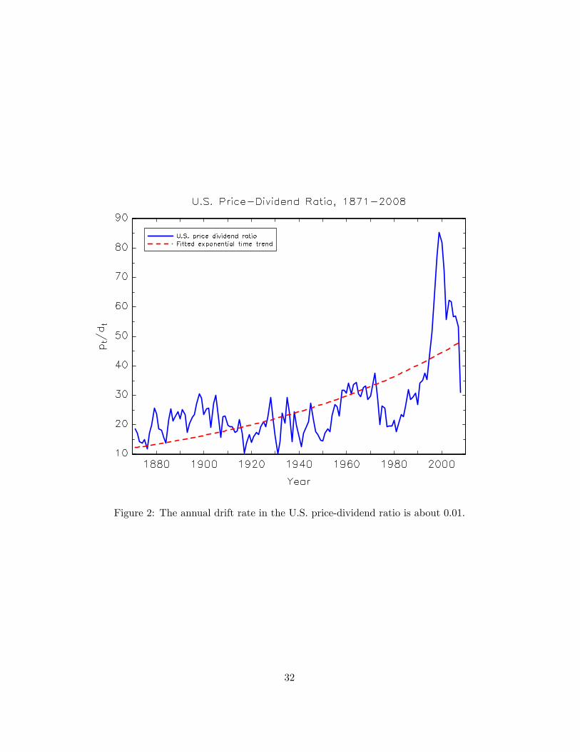
Figure 2: The annual drift rate in the U.S. price-dividend ratio is about 0.01.

32

Figure 3: Properties of the near-rational equilibrium.

33

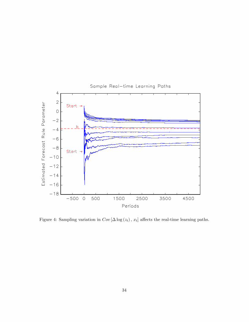
Figure 4: Sampling variation in Cov [� log (zt) ; xt] a¤ects the real-time learning paths.

34

Figure 5: Left panels: price-dividend ratio. Right panels: net equity return.

35