Rational Addiction Evidence from Carbonated Soft Drinks...

Rational Addiction Evidence from Carbonated Soft Drinks

Xiaoou Liu and Rigoberto Lopez

Department of Agricultural and Resource Economics

University of Connecticut

W.B. Young Building, 1376 Storrs Road

Storrs, CT 06269

June 30, 2009

Contributed Paper prepared for presentation at the International Association of Agricultural

Economists Conference, Beijing, China, August 16-22, 2009.

Copyright 2009 by the authors. All rights reserved. Readers may make verbatim copies ofthis document for non-commercial purposes by any means, provided that this copyright noticeappears on all such copies.

ABSTRACT

Rational Addiction Evidence from Carbonated Soft Drinks. XIAOOU LIU (Email: liuxi-

[email protected], Department of Agricultural and Resource Economics, Storrs, CT

06269) RIGOBERTO LOPEZ (Professor and Department Head, Department of Agricultural

and Resource Economics, Storrs, CT 06269)

This paper applies the Becker-Murphy (1988) theory of rational addiction to the case of

carbonated soft drinks, using a time-varying parameter model and scanner data from 46 U.S.

cities. Empirical results provide strong evidence that carbonated soft drinks are rationally

addictive, thus opening the door to taxation and regulation. Taking rational addition into

account, estimated demand elasticities are much lower than previous estimates using scanner

data.

Key words: rational addiction, carbonated soft drinks, time-varying parameter model

i

INTRODUCTION

Addiction is commonly defined as excessive physical or psychological dependence to a sub-

stance or activity. From a public policy perspective, addiction is an important issue as

excessive consumption of addictive commodities lead to negative health outcomes. This

chapter is the first to focus on addiction to carbonated soft drinks (herein CSDs) whose ex-

cess consumption can contribute to the obesity epidemic and health related complications.

If a product is addictive, then this provides a rationale for government intervention.

Economists have a long standing interest in modeling addictive processes due to their

important in explaining certain consumption behaviors that seem to contradict the ratio-

nality basis of economics. From an economic perspective, addictions are always associated

with two conditions: reinforcement and tolerance. Reinforcement refers to the fact that

more consumption of addictive commodities at present will lead to more consumption in the

future. Tolerance implies that more consumption at present will lead to lower future utility

of a given amount of future consumption.

In a milestone paper, Becker and Murphy (1988, herein BM) theoretically illustrate that

many addictions previously thought to have been irrational are consistent with consumer

choice theory given stable consumer preferences. The study points out that addictive behav-

ior is rational if an increase in current consumption of an addictive product increases future

consumption of that product. In the BM model, both past and future consumptions raise

the marginal utility of current consumption. Thus, to test a rational addiction hypothesis is

equivalent to ask whether consumption today is dependent on both past consumption and

future consumption.

To test the theoretical model of rational addiction, Becker, Grossman, and Murphy (1994,

herein BGM) examined whether lower past and future prices for cigarettes raise current

cigarette consumption. Furthermore, empirical applications of the BM framework have also

1

been conducted on cigarettes (Baltagi and Griffin, 2001), alcohol (Waters and Sloan, 1995;

Grossman, Chaloupka, and Sirtaian, 1998; Bentzen and Eriksson, 1999; Baltagi and Griffin,

2002), caffeine (Olekalns and Bardsley, 1996), and Richards, Patterson and Tegene (2007)

on nutrient consumption.

This chapter applies the BM rational addiction model to carbonated soft drinks in the

United States. This product provides an excellent case study for the following reasons. First,

addiction is apparent given the fact that CSDs per capita consumption in U.S. is more than

tripled since 1975 (Allshouse, 2004).1 Second, excessive consumption of CSDs has direct

implications for the obesity epidemic and type 2 diabetes in children whose incidence has

paralleled the rise in consumption of CSDs, particularly via the consumptions of excess

calories (Harnack, Stang and Story, 1999 and Apovian, 2004). Third, this chapter is the first

study to test rational addiction nature of carbonated soft drinks, thus adding to the scarce

economic literature on food as an addiction.

The first objective of this study is to present evidence whether or not CSDs are addictive.

This is equivalent to test the hypothesis that if higher past and future prices raise current

consumption of CSDs . The second objective is to assess the potential of price policies that

relate health problems to CSDs consumption, as consumption of an addictive product is

irresponsive to market prices so mechanic adjustments of a market are not efficient to keep

consumption at a healthy level.

To achieve the objectives, this chapter empirically implements the BM framework using a

time-varying parameter model (Kim, 2006) and supermarket scanner data from 46 U.S. cities.

Empirical results reveal that CSDs are rationally addictive as past and future consumptions

signicantly increase current consumption, resulting in signicantly lower price elasticities than

those found in previous studies that do not take addiction into account. Thus, results indicate

1The increasing pattern is observed to parallel to the increases of obesity and type 2 diabetes, especiallyamong children and adolescents.

2

that, because of rational addiction behavior, CSD consumption is highly irresponsive to

changes in market prices and highlights the need of incorporating an inter-temporal linkage

in CSDs demand modeling. Ultimately, the results confirm the candidacy of CSDs for

government intervention given its addictive nature.

LITERATURE REVIEW

The study of rational addiction draws back to the attempts to model habit persistence. For

example, Pollak (1970) postulates the parameters of consumers’ utility function to depend

in a specific way on past consumption and derives a dynamic demand function. He con-

cludes that if goods are habit persistent, consumers’ current preference will depend on the

consumption pattern in the past. Ryder and Heal (1973) find the similar results that con-

sumers’ satisfaction from a given bundle of goods depend not only on that bundle but also

on past consumption.

Before the idea of rational habit formation is first discussed by Spinnewyn (1981), the

studies of habit persistent only focus on the impact of past consumption on current con-

sumption. The idea of considering habit persistence as a rational behavior proves that if

consumers’ taste changes endogenously through habit stocks that depend on past consump-

tion, the current consumption of a rational consumer will depend on the future habit forming.

This scope finally leads to the emergence of studies in rational addiction.

The concept of rational addiction is introduced by Stigler and Becker (1977), and further

developed by Iannaccone (1984, 1986). In a rational addiction framework, although con-

sumers are aware of the cost of addictive consumption, they still make the addiction choice

because gains from addiction exceed costs of being addictive in the future. Based on this

rationality, Becker and Murphy (1988) derive the explicit long-run and short-run demand

functions for addictive products and relate temporarily stressful events to permanent addic-

3

tions. Stronger addiction to a product requires a greater effect of past consumption of the

product on current consumption. This powerful complementariness between past consump-

tion and current consumption cause steady-state consumption levels of an addictive product

to be unstable. Thus, any small deviations from the consumption at an unstable steady

state can lead to large cumulative rises or to rapid falls in consumption over time.

Gruber and Koszegi (2001) criticize BM model by constraining the analysis to time

consistent consumers. The evidence from studies in psychology shows that consumers tend to

discount less for far futures than closer futures and thereby consumers are time-inconsistent.

From this aspect, the rationality hypothesis of an addiction is rejected as the inconsistent

discounting pattern raises the specter of intra-personal conflict over decisions for future.

However, this model cannot be distinguished from BM model empirically.

BGM (1994) is the first empirical study of rational addition. The study concludes that

smoking is rationally addictive by showing that the current cigarettes consumption depends

on both past consumption and future consumption. The estimates show strong evidence of

reinforcement and tolerance effects regarding cigarette consumption. The estimated long-run

price elasticity at the sample mean of BGM data is 1.8 times more than the short-run price

elasticity and reveals the fact that a permanent price reduction have moro significant effect

in long run rather than in short run.

Besides the typically considered addictive products, a variety of empirical studies have

been done on food addiction to respond the concerns raised by harmful health consequence of

excessive food consumption. Cawley (1999) analyzes consumers propensity of food addiction,

and Grootendorst (2004) find that that milk and eggs are also rationally addictive. Richards

et al. (2007) test a rational addiction hypothesis for specific macronutrients in foods and

find a particularly strong addiction to carbohydrates. This study suggests that a price

based policy, or sin tax that change the expected future costs and benefits of consuming

carbohydrate-intensive foods may be effective in controlling excessive nutrient intake.

4

THEORETICAL MODEL

Following Becker, Grossman and Murphy (1994), an infinite lived representative consumer

with wealth A0 is assumed to maximize the sum of his lifetime utilities respect to a budget

constraint, i.e.,

max∞∑

t=1

θt−1U(Ct, Ct−1, Zt),

with C0 = C0 and subject to:∑∞

t=1 βt−1(Zt + ptCt) = A0. U is a quadratic utility function

of the rationally addicted consumer, Ct is the amount of CSDs consumption at time t, Ct−1

is the amount of CSDs consumption at time t− 1, and Zt is the amount of a non-addictive

composite product consumption at time t. The discount factor θ is equal to 11+r

, where r is

real interest rate. Zt is taken as numeraire and pt denotes the price of CSDs. Consumption

Ct is assumed to have no income effect.2

The first-order conditions are:

Uz(Ct, Ct−1, Zt) = λ, (1)

U1(Ct, Ct−1, Zt) + θU2(Ct+1, Ct, Zt+1) = λpt. (2)

Equation (1) shows that marginal utility of non-addictive consumption in each period Uz is

equivalent to the marginal utility of wealth λ. Equation (2) illustrates that the marginal

utility of wealth multiplied by the current price equals the marginal utility of current CSD

consumption, U1, plus the discounted marginal effect of current consumption at the t on the

utility at time t + 1, U2 is summed to be negative because of the harmful health effects of

excessive CSD consumption.

To solve the first-order conditions, Becker et al. (1994) assumed a linear quadratic utility

2This assumption indicates that consumption over time has no effect on the present value of wealth A0.

5

function of Zt, Ct, Ct−1 as:

U(Zt, Ct, Ct−1) = αzZt +αzz

2Z2

t + α1Ct +α11

2C2

t + α2Ct−1 +α22

2C2

t−1

+ α1zCtZt + α2zCt−1Zt + α12CtCt−1.

After solving the first-order condition for Zt and plugging the result in the first-order condi-

tion for Ct, a linear difference equation for current CSDs consumption is obtained as

Ct = β1Ct−1 + θβ1Ct+1 + β2pt (3)

where

β1 =−(α11αzz − α1zα2z)

(α11αzz + α21z) + θ(α22αzz − α2

2z)

β2 =−(αzzλ)

(α11αzz + α21z) + θ(α22αzz − α2

2z)

Equation (3) illustrates that current consumption of a rationally addictive product is a

function of past consumption Ct−1 , future consumption Ct+1, and current price pt. β2 is

negative because of the concavity assumption of utility function. θ appears as a coefficient

for both past and future consumption. To meet the reinforcement and tolerance conditions

of rational addiction, a positive value of β1 is required to capture the phenomena that both

of past and future consumptions raise current consumption. Additionally, the greater of β1

is, the more addictive the product is.

The solution for the difference equation in (3) is:

Ct =1

β1φ1(φ2 − φ1)

∞∑s=1

φs1h(t+ s) +

1

β1φ2(φ2 − φ1)

∞∑s=0

φ−s2 h(t− 2) (4)

+1

φt2

(C0 − 1

β1φ1(φ2 − φ1))∞∑

s=1

φs1h(s)), (5)

6

where

h(t) = β0 + β2pt−1,

φ1 =1−

√(1− 4β2

1θ)

2β1

,

φ2 =1 +

√(1− 4β2

1θ)

2β1

.

with 4β21θ < 1 for stability.

The impact of a temporary CSD price change at time m on CSD consumption at time t

can then be derived as3:

dCt

dpm

∣∣∣∣m>t

=β2φ

m−t1

β1(φ2 − φ1)

[1− (

φ1

φ2

)t

], (6)

dCt

dpm

∣∣∣∣m<t

=β2φ

m−t2

β1(φ2 − φ1)

[1− (

φ1

φ2

)m

], (7)

dCt

dpt

=β2

β1(φ2 − φ1)

[1− (

φ1

φ2

)t

]. (8)

β1 determines the signs of equation (6)-(8). Equation (8) is used to compute a completely

unanticipated own price effect by setting t or m equal to 1, while the fully anticipated price

effect is obtained by setting t or m equal to infinity. For addictive products, anticipated

future price increases reduce current consumption, as consumption at different periods are

compliments.

The permanent price reduction beginning at time t effects on the current consumption

is given by:

dCt

dp∗t=

β2[1− (φ1/φ2)t]

β1(1− φ1)(φ2 − φ1).

3The derived prices effect from equation (5) is a temporary price effect because the derivation of equation(6)-(8) assumes prices in other periods are held constant.

7

By setting t goes to infinity, the equation becomes

dCt

dp∗t=

β2

β1(1− φ1)(φ2 − φ1),

and gives a short-run price effect.4

The effect of a permanent price reduction over all periods on the consumption Ct is

dCt

dp=

β2φ−t2

β1(φ2 − φ1)

[φt

2

φ2 − 1− 1− (φ1/φ2)

t

β1(1− φ1)(φ2 − φ1)

]+

β2[1− (φ1/φ2)t]

β1(1− φ1)(φ2 − φ1). (9)

Equation (9) is used to calculate the long run price effect of the permanent price reduction

by setting t goes to infinity:

dC∞dp

=β2

β1(1− φ1)(φ2 − 1).

In BM’s rational addiction framework, permanent price changes of an addictive product

have a small short-run effect on current consumption, which explains a general perception

that addicts do not respond much to price changes. Long-run demand for addictive products

tends to be more elastic than short-run demand. Furthermore, a permanent price change

shows greater impact on current consumption than a temporary price change.

EMPIRICAL MODEL

For the empirical implementation, this study adopts a time-varying parameter model. The

model allows the estimated coefficients to vary over time by incorporating the information

about consumers choice over time. Thus, the estimated time path of rational addiction coef-

ficient β1 not only provides more information about the changes in degree of addictiveness,

4Becker and Murphy (1988) defines a short-run price effect as the effect of a completely unanticipatedpermanent price reduction (including prices of all future time periods) on current consumption.

8

but also incorporates the changing degrees of uncertainty over time on rationally addictive

preferences. Furthermore, estimates of the time-varying discount factor θ could be used to

test whether consumers have a time-consistent discount factor, as assumed in the rational

addiction framework.

An empirical equation for panel data can be written as follows:

cit = λi + β1tci,t−1 + β1tθtci,t−1 + β2tpit + β4tyit +mit, (10)

where the subscript i denotes the ith cross-sectional unit and the subscript t denotes the tth

period. cit is CSDs consumption in period t, and pit is the retail price, yit is income, and mit

is an unobserved shock. To capture the variation of marginal utility of wealth among cities,

a city level fixed effect variable λi is included, as suggested both by BGM and Hsiao (1986).

λi can be eliminated by taking the first difference of equation (10):

∆Ct = (β1t − β1,t−1∆Ct−1 + (β1tθt − β1,t−1θt−1)∆Ct+1 (11)

+ (β2t − β2,t−1)∆Pt + (β4t − β4,t−1)∆Yt + ∆Mt,

where

∆Ct = [∆c1t, . . . ,∆cit, . . . ,∆cnt]′,

∆Pt = [∆p1t, . . . ,∆pit, . . . ,∆pnt]′,

∆Yt = [∆y1t, . . . ,∆yit, . . . ,∆ynt]′,

∆Mt = [∆m1t, . . . ,∆mit, . . . ,∆mnt]′.

Following Kim (2006), the forward-looking behavior Ci,t+1 is modeled as

∆Ct+1 = β0t + β3tEt(∆Pt+1), (12)

9

where Et(·) refers to the expectation formed conditional on information set at time t.

By plugging equation (12) into equation (12) the change of current consumption becomes

∆Ct = (β1tθt − β1,t−1θt−1)β0t + (β1t − β1,t−1)∆Ct−1 (13)

+ (β2t − β2,t−1)∆Pt + (β1tθt − β1,t−1θt−1)β3t∆Pt+1 + (β4t − βt,t−1)∆Yt + et,

with

βjt = a0j + a1jβj,t−1 + εjt, εjt ∼ i.i.d. N(0, σ2ε,j) (14)

θt = a0,5 + a1,5θt−1 + ε5,t, ε5,t ∼ i.i.d. N(0, σ2ε,5) (15)

for j = 1, 2, 3, 4. The new error terms et is equal to (−(β1tθt − β1,t−1θt−1)β3t(∆Pt+1 −

E(∆Pt+1)) + ∆Mt). The discount factor θt is constrained between 0 and 1.

Furthermore, to model the time-varying variance of unobserved shocks, the model as-

sumes the distribution of et following a GARCH (1,1) process, i.e.,

et|Ψt−1 ∼ N(0, σe,t), (16)

σ2e,t = α0 + α1e

2t−1 + α2σ

2e,t−1, (17)

where Ψt−1 refers to information up to t− 1.

EMPIRICAL ISSUES

The empirical implementations to equation (14) raise three empirical issues: endogeneity,

non-linearity, and heteroscedasticity. This section will propose a solution algorithm to these

issues before conducting an estimation.

10

Endogeneity

Equation (14) implies that the lagged variable ∆Ct−1 is correlated with ∆Mt, even under

the assumption that ∆Mt is not serially correlated. Rivers and Voung (1988) suggests a

two-step procedure to solve this issue. The first step is to regress the endogenous variable

∆Ct−1 against exogenous variables. The estimated regression is used to create a new variable

∆Ct−1. The second step is to estimate the objective function with ∆Ct−1 instead of ∆Ct−1.

The second endogeneity issue is caused by the correlation between regressor ∆Pt+1 and

the disturbance term et, as part of et is constructed to contain ∆Pt+1. Kim (2006) suggests

a general approach to solve this issue by decomposing et into two uncorrelated parts. The

first step to proceed this approach is to formulate ∆Pt+1 with a set of instrument variables

It:

∆Pt+1 = I ′tδt + vt, vt ∼ N(0, σ2v,t) (18)

with

δt = b0 + b1δt−1 + ut, ut ∼ i.i.dN(0,Σu), (19)

σ2v,t = c0 + c1v

2t−1 + c2σ

2v,t−1. (20)

By construction, the relationship between the endogenous regressors ∆Pt+1 and the vector

of IV It is also modeled with the time-varying coefficient δt and an unobserved heteroscedastic

shock vt, which is specified to follow a GARCH (1,1) process. These specifications implement

that uncertainty associated with future prices can vary over time with a time variation in

σt, even in absence of heteroscedasticity in vt.

The second step is to decompose ∆Pt+1 into two components: predicted component and

prediction error component; i.e.,

∆Pt+1 = E(∆Pt+1|Ψt−1) + vt|t−1,

11

vt|t−1 = Ω1/2t|t−1v

∗t , v

∗t ∼ i.i.d.N(0, 1)

where Ψt−1 is information up to time t−1 and Ωt|t−1 is the time-varying conditional variance

for prediction error. Both vt|t−1 and Ωt|t−1 can be obtained by estimating equation (18)-(20)

through a maximum likelihood procedure based on Harvey et al.’s (1992) modified Kalman

filter.

The prediction errors v∗t is then standardized by assuming the covariance structure be-

tween v∗t and et as: v∗t

et

∼ N

0

0

, 1 ρσe,t

ρσe,t σ2e,t

,

where ρ is a constant correlation coefficient. Apply the Cholesky decomposition to the

covariance matrix, resulting in the following relationship between v∗t and et:

v∗t

et

=

1 0

ρσe,t

√1− ρ2σe,t

εt

wt

, εt

wt

∼ i.i.d.N

0

0

, 1 0

0 1

, (21)

Rewrite equation (21) as:

et = ρσe,tv∗t + w∗t , w

∗t ∼ N(0, (1− ρ2)σ2

e,t), (22)

where w∗t is uncorrelated with v∗t .

After the transformations, equation (22) decomposes et in equation (14) into two com-

ponents: v∗t , which is correlated with ∆Pt+1; and w∗t , which is uncorrelated with any of

12

regressors. Plugging equation (22) into equation (14), equation (14) then becomes

∆Ct = (β1tθt − β1,t−1θt−1)β0t + (β1t − β1,t−1)∆Ct−1 (23)

+ (β1tθt − β1,t−1θt−1)β3t∆Pt+1 + (β2t − β2,t−1)∆Pt

+ (β4t − β4,t−1)∆Yt + ρσe,tv∗t + w∗t ,

where v∗t is now considered as an additional regressor. The new disturbance term w∗t is

uncorrelated with any of the regressors.

Nonlinearity and heteroscedasticity

The coefficients β1t, θt, β0,t, β3t in equation (24) are not identified without further implemen-

tations, as they appear in the equation through multiplication. To solve this issue, rewrite

the non-linear equation (24) and (14)-(17) as

∆Ct = f(xt; βt) + ρσe,tv∗t + w∗t w

∗t ∼ N(0, (1− ρ2)σ2

e,t), (24)

with

βt = µ+ Fβt−1 + εt εt ∼ i.i.d.N(0,Σε),

σ2e,t = α0 + α1e

2t−1 + α2σ

2e,t−1,

where βt = [β0t β1t β2t β3t β4t θt]′, Σε is a diagonal matrix, and

f(xt; βt) = (β1tθt − β1,t−1|t−1θt−1|t−1)β0t + (β1t − β1,t−1|t−1)∆Ct−1 (25)

+ (β1tθt − β1,t−1|t−1θt−1|t−1)β3t∆Pt+1 (26)

+ (β2t − β2,t−1|t−1)∆Pt + (β4t − β4,t−1|t−1)∆Yt, (27)

13

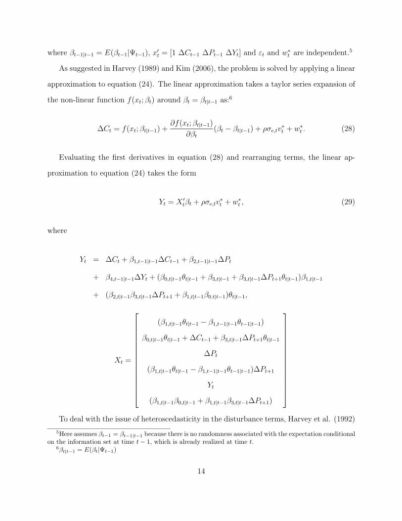
where βt−1|t−1 = E(βt−1|Ψt−1), x′t = [1 ∆Ct−1 ∆Pt−1 ∆Yt] and εt and w∗t are independent.5

As suggested in Harvey (1989) and Kim (2006), the problem is solved by applying a linear

approximation to equation (24). The linear approximation takes a taylor series expansion of

the non-linear function f(xt; βt) around βt = βt|t−1 as:6

∆Ct = f(xt; βt|t−1) +∂f(xt; βt|t−1)

∂βt

(βt − βt|t−1) + ρσe,tv∗t + w∗t . (28)

Evaluating the first derivatives in equation (28) and rearranging terms, the linear ap-

proximation to equation (24) takes the form

Yt = X ′tβt + ρσe,tv∗t + w∗t , (29)

where

Yt = ∆Ct + β1,t−1|t−1∆Ct−1 + β2,t−1|t−1∆Pt

+ β4,t−1|t−1∆Yt + (β0,t|t−1θt|t−1 + β3,t|t−1 + β3,t|t−1∆Pt+1θt|t−1)β1,t|t−1

+ (β2,t|t−1β3,t|t−1∆Pt+1 + β1,t|t−1β0.t|t−1)θt|t−1,

Xt =

(β1,t|t−1θt|t−1 − β1,t−1|t−1θt−1|t−1)

β0,t|t−1θt|t−1 + ∆Ct−1 + β3,t|t−1∆Pt+1θt|t−1

∆Pt

(β1,t|t−1θt|t−1 − β1,t−1|t−1θt−1|t−1)∆Pt+1

Yt

(β1,t|t−1β0,t|t−1 + β1,t|t−1β3,t|t−1∆Pt+1)

To deal with the issue of heteroscedasticity in the disturbance terms, Harvey et al. (1992)

5Here assumes βt−1 = βt−1|t−1 because there is no randomness associated with the expectation conditionalon the information set at time t− 1, which is already realized at time t.

6βt|t−1 = E(βt|Ψt−1)

14

suggests to include w∗t in the state-space equation (29) to formulate

Yt = [X ′t 1]

βt

w∗t

+ ρσe,tv∗t = X ′tβt + ρσe,tv

∗t , (30)

where βt

w∗t

=

µ

0

+

F 0

0′6 0

βt−1

w∗t−1

+

εt

w∗t

, εt

w∗t

∼ N

06

0

, Σε 06

0 (1− ρ2)σ2e,t

,

and

βt = A+Bβt−1 + Vt, Vt ∼ (0, Qt),

which is ultimately estimated equation.

ESTIMATION ALGORITHM

The estimation of equations (30) is conducted using the two-step, maximum likelihood esti-

mator procedure outlined by Heckman (1976). The first step is to estimate equation (18)-(20)

using maximum likelihood estimation based on Harvey et al.’s (1992) modified Kalman filter,

and calculate the one-step-ahead forecast errors, v∗t|t−1. The second step is to use a maxi-

mum likelihood method via the Kalman filter to estimate equation (30) with v∗t as a bias

correction term. The prediction errors v∗t for expected prices enter to the estimation as the

bias correction term to capture the changing degrees of uncertainty associated with future

prices into the estimation of a forward-looking behavior in the rational addiction framework.

15

Thus,

E(e2t−1|Ψt−1) = E(et−1|Ψt−1)2 + E(et−1 − E(et−1|Ψt−1))

2 (38)

= (v∗t−1ρσe,t−1 + E(w∗t−1|Ψt−1))2 (39)

+ E(w∗t−1 − E(w∗t−1|Ψt−1))2, (40)

where E(w∗t−1|Ψt−1) is the last element of βt−1|t−1 and its mean squared error E(w∗t−1 −

E(x∗t−1|Ψt−1))2 is given by the last diagonal element of Λt−1|t−1.

The main database used in this study comes from information Resources, Inc. (IRI),

which is available in the Food Marketing Center at the University of Connecticut. The

data consists of 20 quarterly, city-level observations from 1988 through 1992 over 46 U.S.

metropolitan areas collected from supermarket scanners for a total of 920 observations (20×

46). The variables used in the estimation are volume sales, price, in-store sale promotions,

population, and median income. Consumption is measured as per capita volume sale and

the price is simply the average retail prices at the city level.

EMPIRICAL RESULTS

Table 1 reports the empirical results of hyper-parameters of the first step estimation given

by equations (18)-(20). The dependent variable is future price changes and the explana-

tory variables are current prices changes, current median income changes, and the change

of in-store promotions. Three hyper-parameters b1,1, b1,2 and b1,3 in equation (19), which

associated with the time-varying coefficients in equation (18), are statistically significant at

1% significant level and carry negative signs with absolute values less than 1.

The variance associated with the random shocks for time-varying coefficient of current

change of in-store promotion, Σv,3 is statistically significant at 1% significant level, while

Σv,1 and Σv,2 are not significantly different from zero. The coefficient of lagged time-varying

17

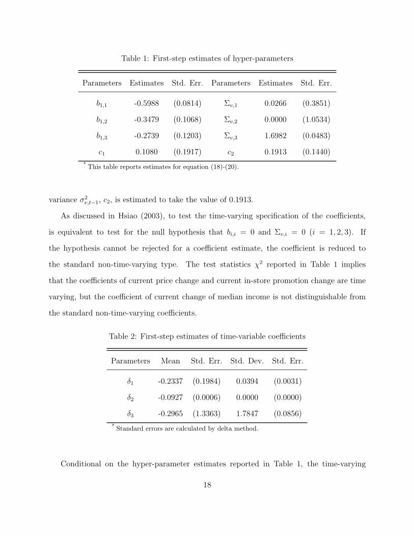
Table 1: First-step estimates of hyper-parameters

Parameters Estimates Std. Err. Parameters Estimates Std. Err.

b1,1 -0.5988 (0.0814) Σv,1 0.0266 (0.3851)

b1,2 -0.3479 (0.1068) Σv,2 0.0000 (1.0534)

b1,3 -0.2739 (0.1203) Σv,3 1.6982 (0.0483)

c1 0.1080 (0.1917) c2 0.1913 (0.1440)

* This table reports estimates for equation (18)-(20).

variance σ2v,t−1, c2, is estimated to take the value of 0.1913.

As discussed in Hsiao (2003), to test the time-varying specification of the coefficients,

is equivalent to test for the null hypothesis that bi,i = 0 and Σv,i = 0 (i = 1, 2, 3). If

the hypothesis cannot be rejected for a coefficient estimate, the coefficient is reduced to

the standard non-time-varying type. The test statistics χ2 reported in Table 1 implies

that the coefficients of current price change and current in-store promotion change are time

varying, but the coefficient of current change of median income is not distinguishable from

the standard non-time-varying coefficients.

Table 2: First-step estimates of time-variable coefficients

Parameters Mean Std. Err. Std. Dev. Std. Err.

δ1 -0.2337 (0.1984) 0.0394 (0.0031)

δ2 -0.0927 (0.0006) 0.0000 (0.0000)

δ3 -0.2965 (1.3363) 1.7847 (0.0856)

* Standard errors are calculated by delta method.

Conditional on the hyper-parameter estimates reported in Table 1, the time-varying

18

Figure 1: Time-varying response of future price to current price

coefficients are calculated by the proposed Kalman filter with equation (31)-(37). Overall,

18 evaluations are obtained for each time-varying coefficient.8 The mean and standard

deviation of each coefficient are shown in table 2. The coefficients of current price change

δ1 and change of median income δ2 are statistically significantly at 5% significant level. The

standard deviation of δ2 takes value 0, which indicates the non-time-varying property of δ2.

Figure 1 depicts the significant time-varying coefficients δ1 with its 95% confidence interval.

The error correction term v∗t is then calculated based on the estimates to proceed the second

step.

The estimates of hyper-parameters from equation (14)-(15) for the second step are re-

ported in Table 3. The dependent variable is changes in current CSD consumption per

capita, and the explanatory variables are changes in past consumption per capita, changes

8The total number of quarters are reduced to 18 because of ∆Pt−1 and ∆Pt+1 are used as explanatoryvariables.

19

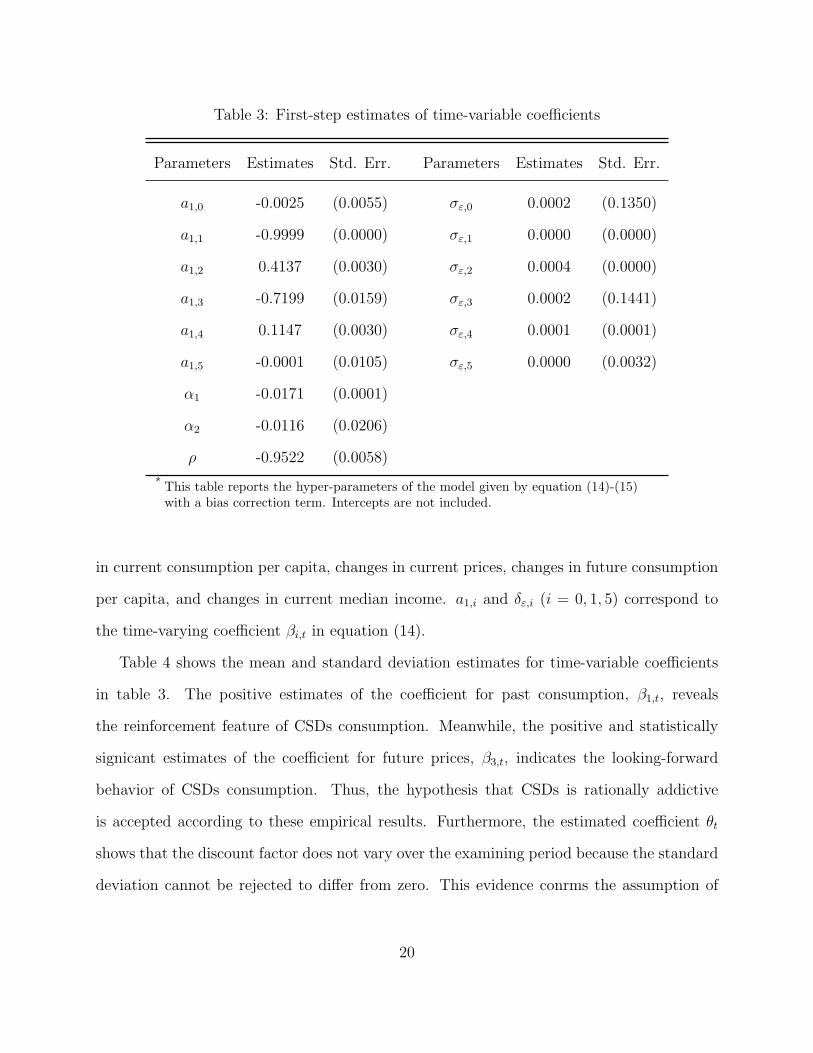
Table 3: First-step estimates of time-variable coefficients

Parameters Estimates Std. Err. Parameters Estimates Std. Err.

a1,0 -0.0025 (0.0055) σε,0 0.0002 (0.1350)

a1,1 -0.9999 (0.0000) σε,1 0.0000 (0.0000)

a1,2 0.4137 (0.0030) σε,2 0.0004 (0.0000)

a1,3 -0.7199 (0.0159) σε,3 0.0002 (0.1441)

a1,4 0.1147 (0.0030) σε,4 0.0001 (0.0001)

a1,5 -0.0001 (0.0105) σε,5 0.0000 (0.0032)

α1 -0.0171 (0.0001)

α2 -0.0116 (0.0206)

ρ -0.9522 (0.0058)

* This table reports the hyper-parameters of the model given by equation (14)-(15)with a bias correction term. Intercepts are not included.

in current consumption per capita, changes in current prices, changes in future consumption

per capita, and changes in current median income. a1,i and δε,i (i = 0, 1, 5) correspond to

the time-varying coefficient βi,t in equation (14).

Table 4 shows the mean and standard deviation estimates for time-variable coefficients

in table 3. The positive estimates of the coefficient for past consumption, β1,t, reveals

the reinforcement feature of CSDs consumption. Meanwhile, the positive and statistically

signicant estimates of the coefficient for future prices, β3,t, indicates the looking-forward

behavior of CSDs consumption. Thus, the hypothesis that CSDs is rationally addictive

is accepted according to these empirical results. Furthermore, the estimated coefficient θt

shows that the discount factor does not vary over the examining period because the standard

deviation cannot be rejected to differ from zero. This evidence conrms the assumption of

20

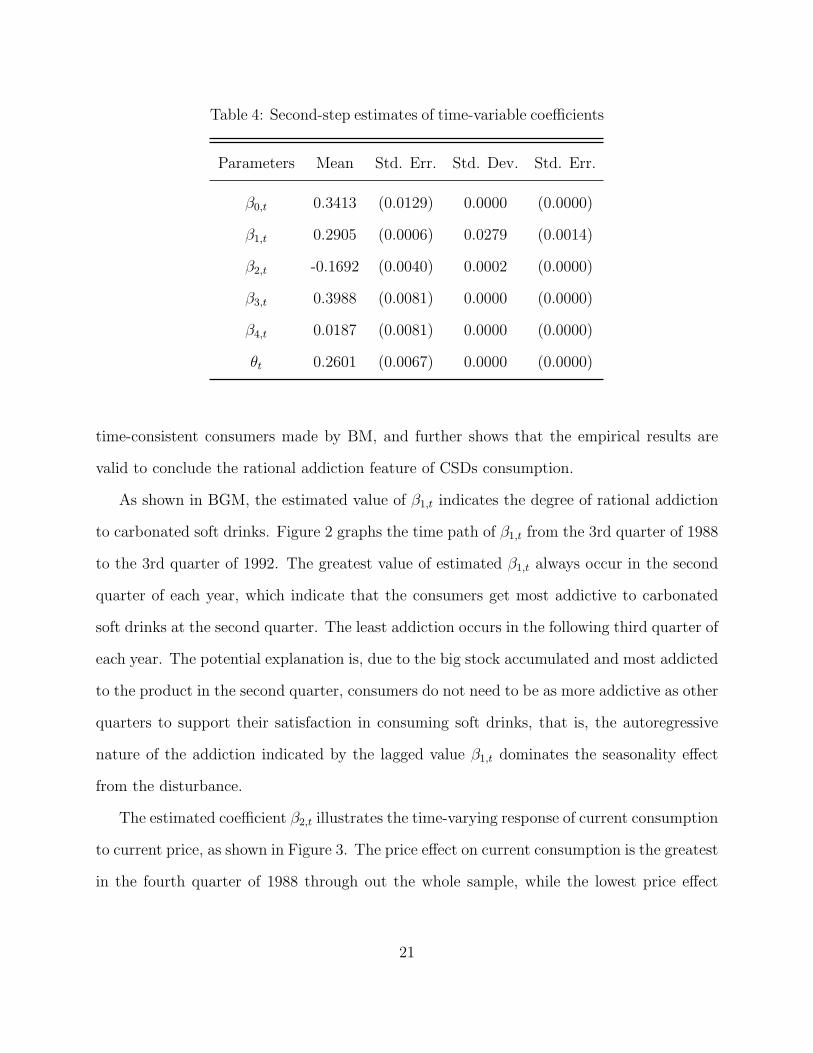
Table 4: Second-step estimates of time-variable coefficients

Parameters Mean Std. Err. Std. Dev. Std. Err.

β0,t 0.3413 (0.0129) 0.0000 (0.0000)

β1,t 0.2905 (0.0006) 0.0279 (0.0014)

β2,t -0.1692 (0.0040) 0.0002 (0.0000)

β3,t 0.3988 (0.0081) 0.0000 (0.0000)

β4,t 0.0187 (0.0081) 0.0000 (0.0000)

θt 0.2601 (0.0067) 0.0000 (0.0000)

time-consistent consumers made by BM, and further shows that the empirical results are

valid to conclude the rational addiction feature of CSDs consumption.

As shown in BGM, the estimated value of β1,t indicates the degree of rational addiction

to carbonated soft drinks. Figure 2 graphs the time path of β1,t from the 3rd quarter of 1988

to the 3rd quarter of 1992. The greatest value of estimated β1,t always occur in the second

quarter of each year, which indicate that the consumers get most addictive to carbonated

soft drinks at the second quarter. The least addiction occurs in the following third quarter of

each year. The potential explanation is, due to the big stock accumulated and most addicted

to the product in the second quarter, consumers do not need to be as more addictive as other

quarters to support their satisfaction in consuming soft drinks, that is, the autoregressive

nature of the addiction indicated by the lagged value β1,t dominates the seasonality effect

from the disturbance.

The estimated coefficient β2,t illustrates the time-varying response of current consumption

to current price, as shown in Figure 3. The price effect on current consumption is the greatest

in the fourth quarter of 1988 through out the whole sample, while the lowest price effect

21

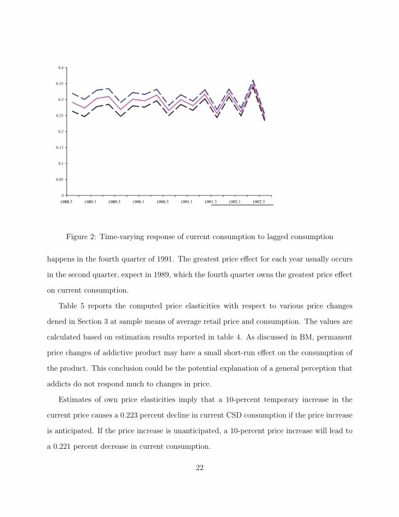
Figure 2: Time-varying response of current consumption to lagged consumption

happens in the fourth quarter of 1991. The greatest price effect for each year usually occurs

in the second quarter, expect in 1989, which the fourth quarter owns the greatest price effect

on current consumption.

Table 5 reports the computed price elasticities with respect to various price changes

dened in Section 3 at sample means of average retail price and consumption. The values are

calculated based on estimation results reported in table 4. As discussed in BM, permanent

price changes of addictive product may have a small short-run effect on the consumption of

the product. This conclusion could be the potential explanation of a general perception that

addicts do not respond much to changes in price.

Estimates of own price elasticities imply that a 10-percent temporary increase in the

current price causes a 0.223 percent decline in current CSD consumption if the price increase

is anticipated. If the price increase is unanticipated, a 10-percent price increase will lead to

a 0.221 percent decrease in current consumption.

22

Figure 3: Time-varying response of current consumption to current price

Estimate of the short-run response of current consumption to a permanent price change

is 0.0226, that is, a 10-percent decline in CSD prices leads to a short-run increase in con-

sumption of 0.226 percent. The long-run response of consumption to a permanent price

change is 0.0319, which is about 1.4 times of the short-run price elasticity and indicates that

a 10-percent reduction in price will lead to 0.319 percent increase in CSD.

For the estimates of cross price effects, a 10-percent unanticipated reduction in price at

time t causes an 0.018 percent increase in consumption at time t + 1. The corresponding

price reduction on consumption at time t− 1 is 0.061.

Hence, the estimates in time-varying coefficients and demand elasticities have jointly il-

lustrated that CSDs are rationally addictive because past and future changes in consumption

have statistically signicant effects on current consumption and CSDs consumption is highly

inelastic to market prices. The estimated CSDs demand elasticities in this paper are much

lower than previous estimates using scanner data. For example, Kinnucan et al. (2001) es-

23

Table 5: Average price elasticities for CSD as a rationally addictive

Elasticities SE Elasticities SE

Own price Future price

unanticipated -0.0221 (0.0035) unanticipated -0.0018 (0.0002)

anticipated -0.0223 (0.0033) Past price

Short-run -0.0226 (0.0029) unanticipated -0.0061 (0.0007)

Long-run -0.0319 (0.0060)

timate the own price elasticity of CSDs at approximately 0.1372, Yen et al. (2004) at -0.52,

Zheng and Kaiser (2008) at -0.151 (AIDS model) and -0.164 (Rotterdam Model), and Dube

et al. (2004) at ranging from -2.0 to -3.0 for a brand-level analysis.

CONCLUSIONS AND DISCUSSION

This paper is the first to test and confirm that CSDs are rationally addictive. This conclusion

is based on finding that past and future consumptions have significant effects on current

consumption. Taking this into account leads to significantly lower own price elasticities

of demand for CSDs than found in previous studies that do not take rational addition

into account. Given that CSDs are rationally addictive, with serious health consequences

(e.g., obesity) for consumers, the findings of this paper provide a rationale for government

intervention on behalf of public health.

The analysis presented in this paper could be expanded in several worthwhile directions.

The first is to include an analysis of quitting behavior of rational addiction within the cold

turkey effect discussed in Becker and Murphy (1988) if the stock of consumption is lowered

sufficiently. Another one is to include the existing taxation in the model and analyze the

24

effects of taxation on current consumption of CSDs in a rational addiction framework. The

third is to take into account interpersonal externalities as well as external costs in the design

of optimal intervention policies that go beyond price policies.

REFERENCES

[1] Apovian, C (2004), “Sugar-Sweetened Soft Drinks, Obesity, and Type 2 Diabetes”,

Journal of American Medical Association, 292, pp. 978-979.

[2] Baltagi, B., and J. Griffin (2001), ”The Econometrics of Rational Addiction: The Case

of Cigarettes.”, Journal of Business and Economic Statistics, 19, pp. 449-454.

[3] Baltagi, B., and J. Griffin (2002), ”Rational Addiction to Alcohol: Panel Data Analysis

of Liquor Consumption”, Health Economics, 19, pp. 449-454.

[4] Becker, G. and K. Murphy (1988), ”A Theory of Rational Addiction”, Journal of Po-

litical Economy, 96, pp. 675-700.

[5] Becker, G., M. Grossman and K. Murphy (1994), ”An Empirical Analysis of Cigarette

Addiction”, American Economics Review, 84, pp. 396-417.

[6] Bentzen, J., T. Eriksson and S. Valdemar (1999), ”Rational Addiction and Alcohol

Consumption: Evidence from the Nordic Countries”, Journal of Consumer Policy, 22,

pp. 257-279.

[7] Capps, O. and J. Griffin (1998), “Effect of a Mass Merchandiser on Traditional Food

Retailers”, Journal of Food Distribution Research, 29, pp. 1-7.

[8] Cawley, J. (1999), ”Rational Addiction, the Consumption of Calories and Body Weight”,

Ph.D. Dissertation, University of Chicago.

25

[9] Chaloupka, F. (1991), ”Rational Addictive Behavior and Cigarette Smoking”, Journal

of Political Economy, 99, pp. 722-742.

[10] Chaloupka, F., M. Grossman, and J. Tauras (1998), ”The Demand for Cocaine and

Marijuana by Youth”, NBER working paper No. W6411.

[11] Dube. J-P. (2004), ”Multiple Discreteness and Product Differentiation: Demand for

Carbonated Soft Drinks.”, Marketing Science, 23, pp. 66-81.

[12] Grossman, M., F. Chaloupka and I. Sirtalan (1998), ”An Empirical Analysis of Alcohol

Addiction: Results from the Monitoring the Future Panels”, Economic Inquiry, 36, pp.

39-48

[13] Grossman, M. and F. Chaloupka (1998), ”The Demand for Cocaine by Young Adults:

A Rational Addiction Approach”, Journal of Health Economics, 17, pp. 427-474.

[14] Gruber, J. and B. Koszegi (2001), ”Is Addiction ’Rational’? Theory and Evidence”,

Quarterly Journal of Economics,116, pp. 1261-1303.

[15] Harnack, L., J. Stang and M. Story (1999), “Soft Drink Consumption Among US Chil-

dren and AdolescentsNutritional Consequences”, Journal of the American Dietetic As-

sociation, 99, pp. 436-441.

[16] lannaccone, L. (1984), ”Consumption Capital and Habit Formation with an Application

to Religious Participation.”, Ph.D. dissertation, University of Chicago.

[17] lannaccone, L. (1986), ”Addiction and Satiation”, Economics Letters, 21, pp. 95-99.

[18] Kim, C-J., and C. Nelson (2006), ”Estimation of A Forward-Looking Monetary Policy

Rule: A Time-Varying Parameter Model Using Ex Post Data”, Journal of Monetary

Economics, 53, pp. 1949-1966

26

[19] Kim, C-J., J. Piger, and R. Startz (2008), “Estimation of Markov Regime-Switching

Regression Models with Endogenous Switching”, Journal of Econometrics, 143, pp.

263–273.

[20] Kinnucan, H., Y. Miao, H. Xiao and H. Kaiser (2001), ”Effects of Advertising on U.S.

Non-Alcoholic Beverage Demand: Evidence from a Two-Stage Rotterdam Model.”, Ad-

vances in Applied Microeconomics: Advertising and Differentiated Products, In M.R.

Baye and J.P. Nelson, ed.

[21] Olekalnsand, N. and P. Bardsley (1996), ”Rational Addiction to Caffeine: An Analysis

of Coffee Consumption”, Journal of Political Economy, 104, pp. 1100-1104.

[22] Richards, T., P. Patterson and A. Tegene (2007), ”Obesity and Nutrient Consumption:

A Rational Addiction?”, Contemporary Economic Policy, 25, pp. 309-324.

[23] Spinnewyn, F. (1981), ”Rational Habit Formation.”, European Economics Review, 15,

pp. 91-109.

[24] Stigler, G. and G. Becker (1977), ”De Gustibus Non Est Disputandum.”, American

Economics Review, 67, pp. 76-90.

[25] Waters, T. and F. Sloan (1995), ”Why Do People Drink? Tests of The Rational Addic-

tion Model”, Applied Economics, 27, pp. 727-736.

[26] Yen, S., B. Lin, D. Smallwood and M. Andrews (2004), ”Demand for Nonalcoholic

Beverages: the Case of Low-Income Households”, Agribusiness, 20, pp. 309321.

[27] Zheng, Y. and H. Kaiser (2008), ”Estimating Asymmetric Advertising Response: An

Application to U.S. Nonalcoholic Beverage Demand”, Journal of Agricultural and Ap-

plied Economics, 40, pp. 837-849.

27

[28] Zywicki, T., Holt, D., and Ohlhausen, M. (2004), Obesity and Advertising Policy, 12

GEORGE MASON L. REV. 979.

28

Rational Addiction Evidence from Carbonated Soft Drinks...

Documents

Transcript of Rational Addiction Evidence from Carbonated Soft Drinks...