Ratings Changes, Ratings Levels, and the Predictive Value of Analysts

Ratings Changes, Ratings Levels,and the Predictive Value of Analysts’

Recommendations

Brad M. Barber, Reuven Lehavy, and Brett Trueman∗

We show that abnormal returns to analysts’ recommendations stem from both the ratings levelsassigned and the changes in those ratings. Conditional on the ratings change, buy and strongbuy recommendations have greater returns than do holds, sells, and strong sells. Conditionalon the ratings level, upgrades earn the highest returns and downgrades the lowest. We alsofind that both ratings levels and changes predict future unexpected earnings and the associatedmarket reaction. Our results imply that 1) investment returns may be enhanced by conditioning onboth recommendation levels and changes; 2) the predictive power of analysts’ recommendationsreflects, at least partially, analysts’ ability to generate valuable private information; and 3)some inconsistency exists between analysts’ ratings and the formal ratings definitions issued bysecurities firms.

It has been well established in the academic literature that analysts’ stock recommendations canpredict security returns.1 What has not been established is whether this predictive power stemsfrom the ratings level assigned by analysts or the change in the ratings level (or both). The goalof this paper is to provide insights into the sources of recommendations’ predictive value and,as a consequence, enhance our understanding of how they can best be employed as part of aninvestment strategy.

Virtually all of the research papers to date that analyze recommendation returns focus on eitherratings changes or ratings levels, but not both. Since changes and levels are positively correlated,such analyses cannot generate insights into the source(s) of recommendations’ predictive value.In contrast, we include both recommendation levels and changes in our analysis. This allows usto calculate the stock returns associated with changes in analysts’ ratings, conditional on ratingslevel, and the returns associated with analyst ratings levels, conditional on ratings change. Wefind that both ratings changes and ratings levels have incremental predictive power for securityreturns.

In a recent paper, Jegadeesh et al. (2004) examine both ratings changes and levels. They findthat the magnitude of analyst consensus recommendation changes is significantly associated withfuture returns. In contrast, no significant relation is found between the consensus recommendationlevels, themselves, and future returns (after controlling for other known drivers of stock returns).

This paper has benefited from the comments of the editor (Bill Christie), an anonymous referee, and seminar participantsat Barclays Global Investors and Rice University.

∗Brad M. Barber is a Professor of Finance at University of California, Davis in Davis, California, USA. Reuven Lehavyis a Professor of Accounting at the University of Michigan in Ann Arbor, Michigan, USA. Brett Trueman is a Professorof Accounting at UCLA in Los Angeles, California, USA.

1 See, for example, Stickel (1995), Womack (1996), Barber et al. (2001), Jegadeesh and Kim (2006), and Green (2006).

Financial Management • Summer 2010 • pages 533 - 553

534 Financial Management � Summer 2010

The methodology employed by Jegadeesh et al. (2004), however, makes it unlikely that theyare fully capturing the value of analyst recommendations. They form consensus recommendationlevel and change portfolios only once a quarter. They then measure portfolio returns over thesubsequent six months, with the composition of each portfolio remaining fixed during thatperiod. As Barber et al. (2001) show, portfolio returns are diminished by delaying for a fewweeks the rebalancing of portfolios following consensus recommendation changes, as well as bynot rebalancing portfolios daily.2 It is unclear how Jegadeesh et al.’s methodology impacts theirconclusions.

Our analysis avoids these potential issues. Our return accumulation period begins when ananalyst initiates coverage, reiterates his or her recommendation, or changes it, and ends when asubsequent recommendation is issued or coverage is dropped. This procedure ensures that thereis no delay in the accumulation of recommendation returns.

As a prelude to our main analysis, we compare returns across ratings levels, independent ofwhether a particular recommendation represents an upgrade, downgrade, reiteration, or initiation.We also compare returns across ratings changes, unconditional on whether the recommendationlevel is a buy, hold, or sell. Consistent with findings of Barber et al. (2001), average daily abnormalreturns generally decrease as we move from more favorable to less favorable recommendations.They range from 1.0 and 0.7 basis points for strong buys and buys, respectively, to −2.5 and −2.4basis points for sells and strong sells, respectively.

Returns also generally increase with the favorableness of a recommendation change. Upgradesare associated with an average daily abnormal return of 1.9 basis points versus 0.5 for initiationsand reiterations, and −1.0 for downgrades. The magnitude of an upgrade, however, is not signif-icantly related to average abnormal return. In contrast, average daily abnormal returns decreasewith downgrade magnitude, ranging from −0.7 basis points for downgrades of only one ratingslevel to −1.6 and −4.4 basis points for downgrades of two and three ratings levels, respectively.

Jegadeesh et al. (2004) find that the relation between recommendation level and abnormalreturn becomes insignificant after controlling for price and earnings momentum. To determinewhether the delays that are introduced into their portfolio formation process might be drivingtheir result, we replicate the construction of their price and earnings momentum index. We thenpartition our sample of recommendations into quintiles according to index value. Within eachmomentum quintile, we again find that the average daily abnormal return for buys and strongbuys is reliably greater than that for sells and strong sells (with the difference ranging between2.0 and 3.9 basis points), indicating that recommendation levels have explanatory value for futurereturns, even conditional on price and earnings momentum.

We turn next to an examination of whether ratings changes have predictive value for security re-turns incremental to ratings levels. We do so by computing average abnormal returns to upgrades,downgrades, and initiations/reiterations, conditional on ratings level. For each ratings level, up-grades are associated with the largest average abnormal return and downgrades, the smallest,consistent with ratings changes providing incremental predictive value for security returns overratings levels. With respect to buy ratings, for example, upgrades generate average daily abnormalreturns that are 2.7 basis points greater than that of downgrades, with the difference being reliablypositive. Upgrades to hold outperform downgrades to hold by a significant 1.4 basis points.

We then examine whether ratings levels have predictive value for security returns incrementalto ratings changes. We do so by conditioning on the sign and magnitude of a ratings change andcomparing average abnormal returns across recommendation levels. If levels do have incremental

2 These results are consistent with findings reported in Stickel (1995) and Womack (1996).

Barber, Lehavy, & Trueman � Ratings Changes, Levels, and Analysts’ Recommendations 535

predictive value, we would expect stocks with more favorable ratings to have higher averageabnormal returns than stocks with less favorable ratings.

Conditioning first on upgrades of one ratings level (sometimes referred to below as singleupgrades), we find that stocks rated buy or strong buy generate a significant average abnormalreturn of 2 basis points per day, while stocks rated hold or sell generate an insignificant 0.1 basispoint average daily abnormal return. The difference of 1.8 basis points is reliably positive.3 Forupgrades of two ratings levels (alternatively referred to as double upgrades), we find that stocksrated buy or strong buy are associated with a significant daily average abnormal return of 2.3basis points; the corresponding return for stocks rated hold is an insignificant 0.5 basis points.Again, the difference between these two returns is reliably positive.

Conditioning on downgrades of one ratings level (sometimes referred to as single downgrades),the stocks rated sell or strong sell generate a significantly negative average daily abnormal returnof −3.4 basis points, while those rated buy are associated with an insignificant average dailyabnormal return of −0.5 basis points. The difference of −2.9 basis points is quite large and reliablynegative. For downgrades of two ratings levels (alternatively referred to as double downgrades),stocks rated sell or strong sell generate a significant average daily abnormal return of −2.9basis points; for stocks rated hold, the corresponding return is −1.4 basis points. The differenceis reliably negative. Overall, these results strongly suggest that ratings levels have incrementalpredictive value for security returns over ratings changes.4

Consistent with our return results, we find that both ratings levels and ratings changes predict themagnitude of, as well as the price reaction to, future unexpected earnings. This is not surprising,given that earnings are a principal driver of stock prices; the ability to predict security returns alsoshould be reflected in an ability to forecast unexpected earnings. Our test consists of regressingunexpected earnings, and separately the price reaction to unexpected earnings, on ratings levels,ratings changes, and several control variables. Both levels and changes enter significantly intothe two regressions.

Our results yield a number of important insights. First, they suggest the potential for investorsto enhance expected returns by conditioning their investment strategies on both recommendationlevels and changes, rather than on just one or the other. This potential for improved returns isillustrated in Figure 1, which plots the cumulative daily raw returns to 1) a levels-only hedgestrategy of purchasing all stocks rated buy or strong buy and selling short all stocks rated sellor strong sell, 2) a changes-only hedge strategy of purchasing all upgraded stocks and shortingall downgraded ones, and 3) a levels- and changes-based hedge strategy of purchasing all stocksreceiving a double upgrade to buy or strong buy and shorting all those receiving a doubledowngrade to sell or strong sell. A $1 investment in either a levels-only or a changes-onlystrategy at the beginning of 1986 would have grown to slightly over $7 at the end of 2006. Incontrast, that same $1 invested in a combined levels- and changes-based strategy would havegrown to over $24.5

Second, our results provide insights into the nature of two possible mechanisms by whichratings levels and changes predict future returns. One mechanism is for recommendations to

3 The differences we report occasionally deviate slightly from the differences in individual returns due to rounding.4 In line with these results, Barber et al. (2001) and Boni and Womack (2006) find that the three-day return aroundrecommendation announcement dates varies with ratings level, conditional on ratings change. (The statistical significanceof these findings, however, is not reported.)5 In untabulated results, we find that this combined strategy earns more than either the levels-based or changes-basedstrategy in 18 of the 21 years of our sample period. Our return results abstract from transactions costs (brokeragecommissions, the bid-ask spread, and the possible impact of trades on market prices).


Figure 1. Value of $1 Invested in Recommendation-Based Strategies, January1986 through December 2006

Plotted here are the cumulative raw returns to 1) a levels-only hedge strategy of purchasing all stocks ratedbuy or strong buy, and selling short all stocks rated sell or strong sell; 2) a changes-only hedge strategy ofpurchasing all upgraded stocks and shorting all downgraded ones; and 3) a levels- and changes-based hedgestrategy of purchasing all stocks receiving a double upgrade to buy or strong buy and shorting all thosereceiving a double downgrade to sell or strong sell.

$0

$5

$10

$15

$20

$25

$30

1986

0131

1987

0130

1988

0129

1989

0127

1990

0126

1991

0125

1992

0124

1993

0122

1994

0120

1995

0120

1996

0119

1997

0117

1998

0116

1999

0119

2000

0118

2001

0117

2002

0123

2003

0123

2004

0123

2005

0124

2006

0124

2006

1231

Levels- and Changes-Based Portfolio:

Long: All Buy/Strong BuyShort: All Sell/Strong Sell

Changes-Based Portfolio:Long: All UpgradesShort: All Downgrades

Short: Double Downgrades to Sell/Strong SellLong: Double Upgrades to Buy/Strong Buy

Levels-Based Portfolio:

permanently shift the demand for stocks, even if the recommendations are uninformative. Theother is for recommendations to convey analysts’ valuable private information about the futurefinancial success of the firms they cover (or, equivalently, their superior interpretation of relevantpublic information). In the latter case, recommendations should be predictive of future unexpectedearnings. Moreover, to the extent that prices do not fully and instantaneously adjust to theinformation content of the recommendations, they should also be able to predict the price reactionsto unexpected earnings. Our findings that recommendations (both levels and changes) do havethe ability to forecast future unexpected earnings as well as the associated price reaction providestrong evidence that the predictive power of analysts’ recommendations does not stem solely fromtheir ability to shift investor demand. Rather, it reflects, at least in part, their ability to gatherrelevant private financial information.6

A third insight of our analysis relates to the consistency between analysts’ recommendationsand the formal ratings definitions issued by securities firms. These definitions are quite uniformacross firms. At its core, a buy or strong buy means that an analyst expects the stock price toincrease (sometimes by a certain minimum amount), either on an absolute or relative basis overa specified time (usually the next 12 to 18 months); a sell or strong sell means that the expected

6 A similar conclusion is reached by Loh and Mian (2006).


stock return is negative; and a hold means that the expected return is close to zero.7 Thesedefinitions are independent of the prior recommendation level (if any), implying that realizedrecommendation returns should be independent of whether a recommendation is an upgrade,downgrade, reiteration, or initiation. That this is contradicted by our results strongly suggests thatanalysts do not strictly abide by the formal ratings definitions when issuing recommendations.This observation contributes to the debate over whether analysts’ alleged conflicts of interests (asoutlined in complaints leading up to the 2003 Global Research Analyst Settlement) have led to adivergence between analysts’ stock ratings and their true investment opinions.8

The plan of this paper is as follows. In Section I we describe our sample and research design. Thisis followed in Section II by an examination of the unconditional abnormal returns to strategiesbased on ratings levels and ratings changes. In Section III we investigate the extent to whichthese abnormal returns are robust to controls for price and earnings momentum. The incrementalpredictive value of ratings changes and ratings levels is examined in Sections IV and V. Section VIcontains a summary and conclusions.

I. Sample Selection, Descriptive Statistics, and Research Design

Our initial sample consists of all recommendations on the Zacks database from January 1986through December 1995 and all real-time recommendations on the First Call database fromJanuary 1996 through the end of 2006.9 From this sample, we drop all recommendations onZacks with a start date prior to January 1, 1986, and all recommendations on First Call with astart date prior to January 1, 1996.

Both databases code recommendations using a five-point scale, ranging from 1 for strongbuy to 5 for strong sell. While the databases employ a five-point scale, some brokers choose toissue only three different ratings—the equivalent of buy, hold, and sell—while still others switchbetween a five-point and a three-point scale during our sample period.10 The recommendationsof the brokers who use a three-point scale are sometimes coded in these databases as 1, 3, and 5;in other cases, they are coded as 2, 3, and 4. For uniformity we recode all such recommendationsas 1, 3, and 5.

7 For example, WR Hambrecht defines a buy as a stock that is “expected in absolute dollar terms to appreciate at least10% over the next 6 months,” a hold as a stock that is “expected to appreciate or depreciate in absolute dollar terms lessthan 10% over the next 6 months,” and a sell as a stock that is “expected to depreciate in absolute dollar terms at least10% over the next 6 months.”8 In its complaint against Salomon Smith Barney (SSB), for example, the SEC said that an e-mail written by a directorwho provided research management support “suggested that the common terms SSB used to rate stocks did not meanwhat they said: ‘various people in research and media relations are very easy targets for irate phone calls from clients,reporters, etc. who make a very literal reading of the rating. . . . [I]f someone wants to read the rating system for exactlywhat it says they have a perfect right to do that.’” See Boni and Womack (2002) for an extensive discussion of analysts’alleged conflicts of interests.9 Comparing the IBES recommendation databases of 2002 and 2004, Ljungqvist, Malloy, and Marston (2009) documenta large number of ex post changes to the recommendation records for the 1993-2002 period. They posit that these changesinfluenced some of the conclusions reached by academics using the data. In light of their findings, we conducted a similaranalysis on the First Call database. We find very high consistency between the historical recommendations of databasesproduced in different years, strongly suggesting that First Call does not suffer from the same problem that Ljungqvist,Malloy, and Marston find in IBES.10 Motivated by the implementation of NASD Rule 2711 in September 2002, many brokers switched from five-point tothree-point scales. The rule requires, in part, that each analyst research report disclose the percentage of its outstandingrecommendations that fall into each of three categories—buys, holds, and sells—regardless of whether the brokerinternally uses more than three possible ratings to characterize its recommendations. For an in-depth discussion andanalysis of the switch in ratings scales, see Kadan et al. (2009).


Table I. Transition Matrix of Analyst Recommendations, 1986-2006

This table shows the number of recommendations in our sample, partitioned according to prior and currentrecommendation levels. The number of initiations in the database (first-time recommendations as wellas recommendations for firms that were previously dropped from coverage) is also presented. Below thenumber of recommendations for each partition is the percentage that those recommendations make up of thetotal. Fractional recommendations are rounded to the nearest whole value. Data for 1986-1995 come fromthe Zacks database; for 1996-2006, the First Call database is the source for recommendations.

To Recommendation of

Strong Buy Buy Hold Sell Strong Sell Total

From recommendation ofStrong buy 78,655 45,348 59,388 1,564 2,985 187,940% of total 7.8 4.5 5.9 0.2 0.3Buy 43,335 50,971 54,241 3,686 1,969 154,202% of total 4.3 5.1 5.4 0.4 0.2Hold 47,954 43,616 91,792 14,653 16,480 214,495% of total 4.8 4.4 9.2 1.5 1.6Sell 1,276 3,081 13,941 5,939 4,375 28,612% of total 0.1 0.3 1.4 0.6 0.4Strong sell 2,103 1,569 15,423 4,080 8,417 31,592% of total 0.2 0.2 1.5 0.4 0.8Initiations 127,328 93,516 131,811 13,653 19,469 385,777% of total 12.7 9.3 13.2 1.4 1.9

Total 300,651 238,101 366,596 43,575 53,695 1,002,618

Table I presents the number of recommendations in our sample, partitioned according to theprior recommendation (if any) issued by the brokerage firm and the current recommendation.Of the more than 1,000,000 recommendations in our sample, only 9.8%, or about 97,000, aremovements to, or initiations of, either sell or strong sell. The dearth of such recommendationshas been well documented in the literature and is consistent with analysts’ alleged reluctance toissue negative recommendations on the firms they follow.11 In contrast, revisions to, or initia-tions of, buy or strong buy total over 538,000, or 53.8% of the total number of recommendationannouncements. Upgrades and downgrades make up 17.6% and 20.4%, respectively, of the sam-ple; reiterations of recommendations comprise 23.5%; and initiations account for the remaining38.5% of the total.

Our principal analyses require the calculation of abnormal returns for portfolios of recommen-dations, partitioned according to ratings level and/or ratings change. To understand how thesereturns are calculated, take as an example a portfolio consisting of all stocks rated strong buy.Each such stock enters the portfolio at the close of trading on the day that the strong buy isissued (unless the announcement comes after the market close, in which case the stock enters theportfolio at the close of the following trading day).12 The stock remains in the portfolio through

11 Barber et al. (2006) document the historical pattern in the percentages of buys, holds, and sells for the 1996-June 2003time period.12 By establishing positions at the close of trading, we explicitly exclude the first trading day recommendation returns.We do so to reflect that many investors, especially small ones, likely learn of recommendations only with a delay. Green(2006) estimates that buying (selling) shares at the beginning of the trading day subsequent to the announcement ofan upgrade (downgrade), rather than waiting until the end of the day, would increase returns by approximately 1.5 (2)percentage points.


the close of trading on the day that the brokerage firm removes the strong buy rating (unlessthe recommendation removal is announced after trading hours, in which case the stock drops outof the portfolio at the close on the next trading day).13 If more than one brokerage firm has anoutstanding strong buy recommendation for a particular stock on a given date, then that stockwill appear multiple times in the portfolio on that date, once for each such recommendation. Eachportfolio is rebalanced daily.14

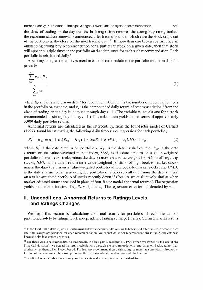
Assuming an equal dollar investment in each recommendation, the portfolio return on date t isgiven by

nt∑

i=1

xit · Rit

nt∑

i=1

xit

, (1)

where Rit is the raw return on date t for recommendation i, nt is the number of recommendationsin the portfolio on that date, and xit is the compounded daily return of recommendation i from theclose of trading on the day it is issued through day t−1. (The variable xit equals one for a stockrecommended as strong buy on day t−1.) This calculation yields a time series of approximately5,000 daily portfolio returns.

Abnormal returns are calculated as the intercept, αj, from the four-factor model of Carhart(1997), found by estimating the following daily time-series regression for each portfolio j:

R jt − R f t = α j + β j (Rmt − R f t ) + s j SMBt + h j HMLt + u j UMDt + ε j t , (2)

where R jt is the date t return on portfolio j, R f t is the date t risk-free rate, Rmt is the date

t return on the value-weighted market index, SMBt is the date t return on a value-weightedportfolio of small-cap stocks minus the date t return on a value-weighted portfolio of large-capstocks, HMLt is the date t return on a value-weighted portfolio of high book-to-market stocksminus the date t return on a value-weighted portfolio of low book-to-market stocks, and UMDt

is the date t return on a value-weighted portfolio of stocks recently up minus the date t returnon a value-weighted portfolio of stocks recently down.15 (Results are qualitatively similar whenmarket-adjusted returns are used in place of four-factor model abnormal returns.) The regressionyields parameter estimates of αj, β j, sj, hj, and uj. The regression error term is denoted by εj.

II. Unconditional Abnormal Returns to Ratings Levelsand Ratings Changes

We begin this section by calculating abnormal returns for portfolios of recommendationspartitioned solely by ratings level, independent of ratings change (if any). Consistent with results

13 In the First Call database, we can distinguish between recommendations made before and after the close because dateand time stamps are provided for each recommendation. We cannot do so for recommendations in the Zacks databasebecause only date stamps are given.14 For those Zacks recommendations that remain in force past December 31, 1995 (when we switch to the use of theFirst Call database), we extend the return calculations through the recommendations’ end-dates on Zacks, rather thanarbitrarily cut them off on December 31. Further, any recommendation outstanding for more than one year is dropped atthe end of the year, under the assumption that the recommendation has become stale by that time.15 See Ken French’s online data library for factor data and a description of their calculation.


in Barber et al. (2001), average daily abnormal returns generally decrease as we move from morefavorable to less favorable recommendation levels.16 As presented in Table II, Panel A, strongbuys and buys are associated with significant average daily abnormal returns of 1.0 and 0.7basis points, respectively. The corresponding returns for sells and strong sells are a significant−2.5 and −2.4 basis points, respectively. The difference between the strong buy and strong sellrecommendation returns, 3.4 basis points, is economically large and reliably positive. The averagedaily abnormal return for holds is not reliably different from zero.

We next calculate abnormal returns for portfolios of recommendations partitioned solely byratings change, independent of ratings level. Table II, Panel B, presents the results. As expected,upgrades generate the largest average daily abnormal return, 1.9 basis points. Downgrades earn thelowest, −1.0 basis points. The difference between these returns, 2.9 basis points, is economicallylarge and significantly greater than zero. Reiterations and initiations generate an insignificant 0.5basis point average daily abnormal return.

Even though upgrades, overall, earn the highest returns, there is no significant associationbetween the magnitude of an upgrade and abnormal returns. As reported in Table II, Panel C,while single and double upgrades are associated with average daily abnormal returns of 1.8 and2.2 basis points, respectively, the difference is not reliably negative. Moreover, upgrades of threeratings levels earn an average abnormal return that is neither significantly different from zero norreliably different from the average abnormal returns to single and double upgrades.

In contrast, a significant relation exists between the magnitude of a downgrade and abnormalreturns (Panel D). Single downgrades generate a significant average daily abnormal return of−0.7 basis points, while double downgrades are associated with a significant average dailyabnormal return of −1.6 basis points. The difference, −0.9 basis points, is reliably negative.Triple downgrades yield the most negative average daily abnormal return, −4.4 basis points.This is 2.8 basis points more negative than that of double downgrades and 3.7 basis pointsmore negative than single downgrades. Both of these differences are economically large andsignificantly negative.

III. Controlling for Price and Earnings Momentum

Jegadeesh et al. (2004) report that the significant relation between ratings level and abnormalreturn disappears after controlling for price and earnings momentum. In this section we replicatethe calculation of their momentum index while employing our portfolio formation methodology(which ensures no delay in the accumulation of recommendation returns) to test whether ratingslevels and ratings changes continue to provide significant explanatory power for abnormal returns.

At the time a recommendation is issued, a momentum index score ranging between 0 and 4 iscompiled. Four variables comprise the index. The first is the price momentum over the periodfrom 252 to 127 trading days (approximately 12 to 6 months) prior to the recommendation date.Denoted by PMOMi

−252,−127, it is equal to the market-adjusted return for recommended stock iover that period

PMOMi−252,−127 =

−127∏

t=−252

(1 + rit ) −−127∏

t=−252

(1 + rmt ), (3)

16 See also Cliff (2007) for an analysis of abnormal returns to portfolios formed solely on the basis of recommendationlevels.


Table II. Unconditional Average Daily Abnormal Returns to Ratings Levels andRatings Changes

This table reports the average daily percentage buy-and-hold abnormal returns (in basis points), and corre-sponding t-statistics, for recommendations partitioned according to ratings level (Panel A), ratings change(Panel B), magnitude of recommendation upgrade (Panel C), and magnitude of recommendation downgrade(Panel D). The difference in returns between various pairs of partitions is also presented. The average dailyabnormal return is the intercept from a regression of the daily portfolio excess return on 1) the excess of themarket return over the risk-free rate, 2) the difference between the daily returns of a value-weighted portfolioof small stocks and one of large stocks, 3) the difference between the daily returns of a value-weighted port-folio of high book-to-market stocks and one of low book-to-market stocks, and 4) the difference betweenthe daily returns of a value-weighted portfolio of stocks recently up and one of stocks recently down.

Panel A. Unconditional Returns to Ratings Levels

Ratings Level Average Daily Abnormal Return (bps) t-StatisticStrong buy 1.0∗∗∗ 3.87Buy 0.7∗∗∗ 3.09Hold −0.2 −0.96Sell −2.5∗∗∗ −5.45Strong sell −2.4∗∗∗ −3.92Strong buy–strong sell 3.4∗∗∗ 5.73Strong buy–hold 1.3∗∗∗ 5.24Strong sell–hold −2.1∗∗∗ 3.90

Panel B. Unconditional Returns to Ratings Changes

Ratings Change Average Daily Abnormal Return (bps) t-StatisticAll upgrades 1.9∗∗∗ 6.95All reit/init 0.5∗ 1.90All downgrades −1.0∗∗∗ −3.49Upgrades–downgrades 2.9∗∗∗ 13.15Upgrades–reit/init 1.4∗∗∗ 8.37Downgrades–reit/init −1.5∗∗∗ −7.41

Panel C. Unconditional Returns across Upgrade Magnitudes

Magnitude of Upgrade Average Daily Abnormal Return (bps) t-StatisticAll single upgrades 1.8∗∗∗ 6.14All double upgrades 2.2∗∗∗ 6.79All triple upgrades 0.5 0.38Single–double −0.4∗ −1.82Double–triple 1.7 1.31Single–triple 1.3 0.97

Panel D. Unconditional Returns across Downgrade Magnitudes

Magnitude of Downgrade Average Daily Abnormal Return (bps) t-StatisticAll single downgrades −0.7∗∗ −2.30All double downgrades −1.6∗∗∗ −4.74All triple downgrades −4.4∗∗∗ −3.10Single–double 0.9∗∗∗ 4.13Double–triple 2.8∗∗ 2.03Single–triple 3.7∗∗∗ 2.67

∗∗∗Significant at the 0.01 level.∗∗Significant at the 0.05 level.∗Significant at the 0.10 level.


where rit is the raw return for stock i on day t relative to the recommendation announcement date,and rmt is the value-weighted market return for that trading day. The second variable is the pricemomentum over the period from 126 to 1 trading day prior to the recommendation date. Denotedby PMOMi

−126,−1, it is given by

PMOMi−126,−1 =

−1∏

t=−126

(1 + rit ) −−1∏

t=−126

(1 + rmt ). (4)

The third measure is the sum of the six most recent consensus analyst earnings forecast re-visions for stock i (as reported monthly in the IBES summary forecast database) prior to therecommendation announcement, each normalized by price.17 Denoted by AFRi

−6,−1, it is givenby18

AFRi−6,−1 =

−1∑

m=−6

(AFim − AFim−1)

Pim−1, (5)

where AFim is the mth most recent consensus analyst forecast of stock i’s current year’s earnings,and Pim is the price of the stock at the time that the consensus is calculated.19 The final componentof the index measures earnings momentum and is defined as the unexpected earnings for themost recent fiscal quarter q prior to the recommendation announcement date, normalized by thestandard deviation of the earnings forecasts. Denoted by SUEiq, it is given by

SUEiq = EPSiq − AFiq

std(AFiq ), (6)

where EPSiq is the realized earnings per share of stock i for quarter q (as reported in the IBESdatabase), AFiq is the most recent consensus analyst quarterly earnings forecast prior to theend of quarter q, and std(AFiq) is the cross-sectional standard deviation of the analyst forecastscomprising the consensus.20

For each of the four measures, we assign a score of one (zero) if its magnitude is above(below) the median for all firms as of the recommendation date. The momentum index (MI) forrecommendation i is the sum of these four scores and ranges between 0 and 4.

For all recommendations with the same MI score, we construct a portfolio of buy- and strong-buy-rated stocks and another of those rated sell or strong sell. Separately, we form a portfolioof stocks receiving upgrades and another of those receiving downgrades. For each of these fourportfolios, we calculate average daily abnormal returns.

Return results for the buy/strong buy and sell/strong sell portfolios are reported in Table III,panel A. For each MI score, the stocks rated buy or strong buy significantly outperform those

17 While Ljungqvist, Malloy, and Marston (2009) find evidence of ex post changes in the IBES recommendation database,they do not find similar irregularities in the database of IBES earnings forecasts.18 For some firms, consensus analyst forecasts are not available on IBES for every month of the prior half year. For thosefirms, we use all of the consensus analyst forecasts available during that period.19 If the recommendation is made after the end of the year, but before the year’s earnings are announced, then the earningsforecasts are for the year just ended.20 The individual analysts’ forecasts that are used to calculate std(AFiq) come from IBES. The variable std(AFiq) is set to0.01 if either there are fewer than two analyst forecasts outstanding or the standard deviation of the analyst forecasts isequal to zero. This definition of unexpected earnings is used by Jegadeesh and Livnat (2006).


Table III. Average Daily Abnormal Returns to Ratings Levels and RatingsChanges, Conditional on Momentum Index Score

This table reports the average daily percentage buy-and-hold abnormal returns (in basis points), and belowthem the corresponding t-statistics, for portfolios of recommendations having the same Momentum Index(MI) score. The four portfolios are 1) that composed of all buy and strong buy recommendations, 2) thatcontaining all sell and strong sell recommendations, 3) that composed of all upgrades, and 4) that containingall downgrades. Also presented is the difference between the average daily abnormal returns of the buy/strongbuy portfolio and the sell/strong sell portfolio as well as the difference between the average daily abnormalreturns of the upgrade and downgrade portfolios. To determine the MI score for each recommendation,we calculate four measures: 1) the cumulative market-adjusted return for the recommended stock over theperiod from 252 to 127 days prior to the recommendation announcement, 2) the cumulative market-adjustedreturn for the recommended stock over the period from 126 days to 1 day prior to the announcement, 3)the sum of the six most recent monthly consensus analyst forecast revisions prior to the recommendationannouncement, normalized by price, and 4) the difference between realized earnings and the consensusanalyst forecast for the most recent quarter prior to the recommendation announcement, scaled by thestandard deviation of the forecasts comprising the consensus. For each measure we assign a score of 1(0) if its value is above (below) the median for all firms as of the recommendation date. The MI score isthe sum of these four individual scores and ranges from 0 to 4. The average daily abnormal return is theintercept from a regression of the daily portfolio excess return on 1) the excess of the market return overthe risk-free rate, 2) the difference between the daily returns of a value-weighted portfolio of small stocksand one of large stocks, 3) the difference between the daily returns of a value-weighted portfolio of highbook-to-market stocks and one of low book-to-market stocks, and 4) the difference between the daily returnsof a value-weighted portfolio of stocks recently up and one of stocks recently down.

Panel A. Returns to Ratings Levels, Conditional on Momentum Index Score

Momentum Buy/ Sell/ Buy/Strong Buy –Index Score Strong Buy Strong Sell Sell/Strong Sell0 (Lowest) 0.8 −3.1∗∗∗ 3.9∗∗∗

(1.57) (−2.59) (3.42)1 1.0∗∗∗ −1.9∗∗∗ 2.9∗∗∗

(2.78) (−2.59) (4.24)2 1.0∗∗∗ −1.4∗ 2.4∗∗∗

(3.46) (−1.68) (2.96)3 1.5∗∗∗ −0.5 2.0∗∗∗

(4.66) (−0.71) (2.84)4 (Highest) 1.5∗∗∗ −1.4 2.9∗∗∗

(3.38) (−1.46) (3.07)

Panel B. Returns to Ratings Changes, Conditional on Momentum Index Score

Momentum Upgrades–Index Score Upgrades Downgrades Downgrades0 (Lowest) 1.5∗∗ −1.4∗∗ 3.0∗∗∗

(2.57) (−2.23) (5.09)1 2.1∗∗∗ −0.7 2.7∗∗∗

(4.64) (−1.49) (7.16)2 2.2∗∗∗ −0.6 2.7∗∗∗

(5.97) (−1.54) (7.64)3 2.3∗∗∗ 0.1 2.1∗∗∗

(5.85) (0.28) (6.03)4 (Highest) 2.5∗∗∗ −0.5 3.0∗∗∗

(4.82) (−1.20) (7.44)

∗∗∗Significant at the 0.01 level.∗∗Significant at the 0.05 level.∗Significant at the 0.10 level.


rated sell or strong sell. The average daily abnormal return difference ranges from 2.0 basispoints (for an MI score of 3) to an economically very large 3.9 basis points (for an MI score of 0).Conditioning on price and earnings momentum, ratings levels continue to have predictive valuefor security returns.

The upgrade and downgrade portfolio return results appear in Panel B. For each MI score,upgrades significantly outperform downgrades. The difference in average daily abnormal returnsranges from 2.1 basis points (for an MI score of 3) to 3.0 basis points (for MI scores of 0 and4). As with ratings levels, ratings changes also provide predictive power for security returns,conditional on price and earnings momentum.

IV. The Incremental Predictive Value of Ratings Changesand Levels

A. Ratings Changes

In this subsection we test whether ratings changes have predictive value for security returnsincremental to that of ratings levels. If they do, then for a fixed ratings level, abnormal returnsshould vary across ratings changes, with upgrades generating the highest returns and downgradesthe lowest. Note that our unconditional return results are insufficient to address this issue sincethe higher average return to upgrades could, in principle, be due to their predominantly beingbuy and strong buy recommendations, while the lower return to downgrades could be due to theirpredominantly being holds, sells, and strong sells.

As presented in Table IV, upgrades do indeed generate the highest returns and downgrades thelowest, conditional on recommendation level, consistent with ratings changes providing incre-mental predictive value for security returns. Within the subset of strong buy recommendations,upgrades are associated with an average daily abnormal return of 2.0 basis points, significantlygreater than the 0.7 basis point average daily abnormal return for reiterations and initiations. Forbuy recommendations, upgrades earn an average daily abnormal return of 2.2 basis points, whiledowngrades generate abnormal returns that are insignificantly different from zero. The differencein returns is reliably positive. With respect to hold recommendations, downgrades earn a reliablynegative average abnormal return of −1.0 basis points; the corresponding return for upgrades isinsignificantly different from zero. The difference in returns is reliably negative. Within the subsetof sell recommendations, downgrades are associated with a significant −3.6 basis point averagedaily abnormal return. Upgrades, in contrast, do not generate a return significantly different fromzero. Despite this, upgrade and downgrade returns are not reliably different from each other. Thisis likely due, at least in part, to the small number of upgrades to sell in our sample. (They compriseless than 0.4% of the total.) The average abnormal return to downgrades, though, is significantlymore negative than that for reiterations and initiations (at −1.6 basis points). Overall, our resultsprovide strong evidence that ratings changes have incremental predictive value for security returnsover ratings levels.

B. Ratings Levels

We next test whether ratings levels have predictive value for security returns incrementalto ratings changes. We do so by holding fixed the sign and magnitude of the ratings changeand examining whether abnormal returns vary with ratings level. If ratings levels do provideincremental predictive value over changes, then upgrades to buy and strong buy should outperform


Table IV. Average Daily Abnormal Return to Ratings Changes, Conditionalon Ratings Level

This table reports the average daily percentage buy-and-hold abnormal returns (in basis points), and belowthem the corresponding t-statistics, for recommendations partitioned according to ratings change, conditionalon ratings level. The difference in returns between various pairs of partitions is also presented. The averagedaily abnormal return is the intercept from a regression of the daily portfolio excess return on 1) theexcess of the market return over the risk-free rate, 2) the difference between the daily returns of a value-weighted portfolio of small stocks and one of large stocks, 3) the difference between the daily returns of avalue-weighted portfolio of high book-to-market stocks and one of low book-to-market stocks, and 4) thedifference between the daily returns of a value-weighted portfolio of stocks recently up and one of stocksrecently down.

Ratings Change Ratings Level

Strong Buy Buy Hold Sell Strong Sell

Upgrades 2.0∗∗∗ 2.2∗∗∗ 0.5 −1.0 –(6.73) (6.85) (1.02) (−0.26) –

Reit/init 0.7∗∗ 0.7∗∗∗ 0.0 −1.6∗∗∗ −2.3∗∗∗

(2.46) (2.65) (−0.09) (−2.84) (−3.35)Downgrades – −0.5 −1.0∗∗∗ −3.6∗∗∗ −2.7∗∗∗

– (−1.44) (−3.04) (−6.32) (−3.31)Upgrades–downgrades – 2.7∗∗∗ 1.4∗∗∗ 2.6 –

– (8.39) (3.54) (0.68) –Upgrades–reit/init 1.3∗∗∗ 1.5∗∗∗ 0.5 0.6 –

(6.10) (5.61) (1.30) (0.16) –Downgrades–reit/init – −1.1∗∗∗ −1.0∗∗∗ −2.0∗∗∗ −0.4

– (−4.38) (−4.39) (−3.05) (−0.44)

∗∗∗Significant at the 0.01 level.∗∗Significant at the 0.05 level.

upgrades to hold and sell. Also, downgrades to buy should outperform downgrades to hold, sell,and strong sell. Note again that our unconditional return results cannot be used to address thisissue as it is possible that the higher average returns to buys and strong buys are due to theserecommendations predominantly being upgrades, while the lower average returns to holds, sells,and strong sells are due to these recommendations predominantly being downgrades.

Our test results are presented in Table V. Turning first to the subset of single upgrade rec-ommendations (Panel A), the average daily abnormal return for buys and strong buys is asignificant 2.0 basis points. In contrast, holds and sells generate an insignificant average daily ab-normal return. The difference between the abnormal returns, 1.8 basis points, is reliably greaterthan zero. Within the subset of single downgrades (Panel B), hold, sell, and strong sell rec-ommendations generate a significant average daily abnormal return of −0.9 basis points. Forthe single downgrades to sell and strong sell, the average daily abnormal return is −3.4 basispoints. In contrast, the corresponding return for downgrades to buy is insignificantly differ-ent from zero. The difference of −2.9 basis points is quite large and significantly less thanzero.

Turning next to the subset of double upgrades (Panel C), the average daily abnormal returnfor buys and strong buys is a significant 2.3 basis points. In contrast, holds earn an insignificantabnormal return. The difference, 1.9 basis points, is reliably greater than zero. For the subset


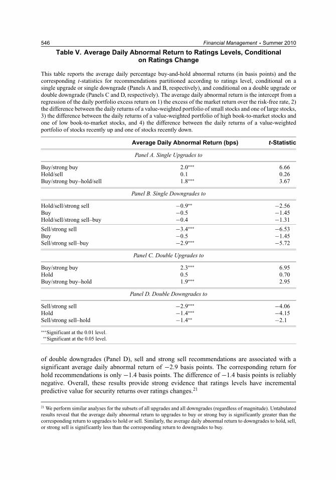
Table V. Average Daily Abnormal Return to Ratings Levels, Conditionalon Ratings Change

This table reports the average daily percentage buy-and-hold abnormal returns (in basis points) and thecorresponding t-statistics for recommendations partitioned according to ratings level, conditional on asingle upgrade or single downgrade (Panels A and B, respectively), and conditional on a double upgrade ordouble downgrade (Panels C and D, respectively). The average daily abnormal return is the intercept from aregression of the daily portfolio excess return on 1) the excess of the market return over the risk-free rate, 2)the difference between the daily returns of a value-weighted portfolio of small stocks and one of large stocks,3) the difference between the daily returns of a value-weighted portfolio of high book-to-market stocks andone of low book-to-market stocks, and 4) the difference between the daily returns of a value-weightedportfolio of stocks recently up and one of stocks recently down.

Average Daily Abnormal Return (bps) t-Statistic

Panel A. Single Upgrades to

Buy/strong buy 2.0∗∗∗ 6.66Hold/sell 0.1 0.26Buy/strong buy–hold/sell 1.8∗∗∗ 3.67

Panel B. Single Downgrades to

Hold/sell/strong sell −0.9∗∗ −2.56Buy −0.5 −1.45Hold/sell/strong sell–buy −0.4 −1.31

Sell/strong sell −3.4∗∗∗ −6.53Buy −0.5 −1.45Sell/strong sell–buy −2.9∗∗∗ −5.72

Panel C. Double Upgrades to

Buy/strong buy 2.3∗∗∗ 6.95Hold 0.5 0.70Buy/strong buy–hold 1.9∗∗∗ 2.95

Panel D. Double Downgrades to

Sell/strong sell −2.9∗∗∗ −4.06Hold −1.4∗∗∗ −4.15Sell/strong sell–hold −1.4∗∗ −2.1

∗∗∗Significant at the 0.01 level.∗∗Significant at the 0.05 level.

of double downgrades (Panel D), sell and strong sell recommendations are associated with asignificant average daily abnormal return of −2.9 basis points. The corresponding return forhold recommendations is only −1.4 basis points. The difference of −1.4 basis points is reliablynegative. Overall, these results provide strong evidence that ratings levels have incrementalpredictive value for security returns over ratings changes.21

21 We perform similar analyses for the subsets of all upgrades and all downgrades (regardless of magnitude). Untabulatedresults reveal that the average daily abnormal return to upgrades to buy or strong buy is significantly greater than thecorresponding return to upgrades to hold or sell. Similarly, the average daily abnormal return to downgrades to hold, sell,or strong sell is significantly less than the corresponding return to downgrades to buy.


C. Levels- and Changes-Based Trading Strategies

The abnormal return findings presented in the prior two subsections suggest that investmentstrategies involving both recommendation levels and changes can outperform those based on eitherlevels or changes alone. We document the return differences among various hedge strategies inColumns 1 and 2 of Table VI. As reported in Panel A, a combined levels- and changes-based hedgestrategy of purchasing stocks receiving single upgrades to buy or strong buy and shorting thosereceiving single downgrades to sell or strong sell generates a significant average daily abnormalreturn of 5.5 basis points.22 In contrast, a changes-only based hedge strategy of purchasing allsingle upgrades and shorting all single downgrades earns an average daily abnormal return of2.5 basis points. The difference between these returns (3.0 basis points, or over 7% annually)is economically large and significantly greater than zero. A levels-only based hedge strategy ofpurchasing all buys and strong buys and shorting all sells and strong sells generates an averagedaily abnormal return of 3.5 basis points. Again, this return is reliably less than that earned bythe combined strategy.

The same pattern is found for double upgrades. As reported in Panel B, a combined levels- andchanges-based strategy of purchasing stocks receiving double upgrades to buy or strong buy andshorting stocks receiving double downgrades to sell or strong sell yields a significant averagedaily abnormal return of 5.2 basis points. The corresponding return to a changes-only basedhedge strategy of purchasing all double upgrades and shorting all double downgrades is 3.8 basispoints. The difference between these two returns is reliably greater than zero. The combinedstrategy’s average daily abnormal return is also reliably greater than that of the levels-only basedstrategy of purchasing all stocks rated either buy or strong buy and shorting all those rated sellor strong sell. These results clearly demonstrate the potential for enhancing investment returnsby conditioning on both recommendation levels and changes rather than on one to the exclusionof the other.23

In Columns 3 through 6 of Table VI, we present the average abnormal returns to the longand short components of each hedge strategy. As the results reveal, the superiority of combinedlevels- and changes-based hedge strategies carries over in large measure to both their long andshort components.24 As shown in Panel A, a strategy of purchasing all single upgrades to buyor strong buy generates significantly higher average abnormal returns than does either a strategyof purchasing all single upgrades or one of purchasing all buys and strong buys. Similarly, a

22 This return deviates slightly from the difference between the returns to single upgrades to buy or strong buy (2.0 basispoints) and single downgrades to sell or strong sell (−3.4 basis points), as given in Table V. This small discrepancy isdue to rounding.23 We alternatively calculate monthly, rather than daily, hedge strategy abnormal returns (by compounding daily returnswithin each month and regressing the monthly returns on the monthly factor returns). In unreported results, we findthat the monthly abnormal returns are of the same order of magnitude as the corresponding daily returns (multiplied by20), albeit slightly smaller in size. All combined levels- and changes-based hedge strategies continue to earn averageabnormal returns significantly higher than those generated by the corresponding levels-only and changes-only basedhedge strategies, with one exception—the average abnormal return to a strategy of purchasing double upgrades to buy orstrong buy and shorting double downgrades to sell or strong sell is not significantly different from that of a strategy ofpurchasing all double upgrades and shorting all double downgrades.24 In untabulated analysis, we generate descriptive statistics on the size composition of the firms in each of the long andshort portfolios. Of note, the portfolio of single downgrades to sell or strong sell is tilted more toward smaller stocks, whilethe portfolio of double upgrades to buy or strong buy is tilted more toward larger stocks, relative to the correspondinglevels-only and changes-only based portfolios. Further, the mean and median market caps of the portfolio of doubledowngrades to sell or strong sell are smaller than those of either the double downgrade or the sell and strong sell portfolio.All these differences, though, pale in comparison to the tilt toward larger stocks evident in the upgrade portfolios, as wellas in the portfolio of buys and strong buys, relative to the downgrade portfolios and the portfolio of sells and strong sells.

548 Financial Management � Summer 2010T

able

VI.

Ave

rag

eD

aily

Ab

no

rmal

Ret

urn

toL

evel

s-an

dC

han

ges

-Bas

edT

rad

ing

Str

ateg

ies

Thi

sta

ble

repo

rts

the

aver

age

daily

perc

enta

gebu

y-an

d-ho

ldab

norm

alre

turn

s(i

nba

sis

poin

ts),

and

next

toth

emth

eco

rres

pond

ing

t-st

atis

tics

,to

vari

ous

long

,sh

ort,

and

hedg

est

rate

gies

invo

lvin

gsi

ngle

upgr

ade

and

dow

ngra

depo

rtfo

lios

(Pan

elA

)an

ddo

uble

upgr

ade

and

dow

ngra

depo

rtfo

lios

(Pan

elB

).T

heav

erag

eda

ilyab

norm

alre

turn

isth

ein

terc

ept

from

are

gres

sion

ofth

eda

ilypo

rtfo

lio

exce

ssre

turn

on1)

the

exce

ssof

the

mar

ket

retu

rnov

erth

eri

sk-f

ree

rate

,2)

the

diff

eren

cebe

twee

nth

eda

ilyre

turn

sof

ava

lue-

wei

ghte

dpo

rtfo

lio

ofsm

all

stoc

ksan

don

eof

larg

est

ocks

,3)

the

diff

eren

cebe

twee

nth

eda

ilyre

turn

sof

ava

lue-

wei

ghte

dpo

rtfo

lio

ofhi

ghbo

ok-t

o-m

arke

tsto

cks

and

one

oflo

wbo

ok-t

o-m

arke

tsto

cks,

and

4)th

edi

ffer

ence

betw

een

the

daily

retu

rns

ofa

valu

e-w

eigh

ted

port

foli

oof

stoc

ksre

cent

lyup

and

one

ofst

ocks

rece

ntly

dow

n.

Hed

ge

Po

rtfo

lioL

on

gP

ort

folio

Sh

ort

Po

rtfo

lio

Ave

rag

eD

aily

t-S

tati

stic

Ave

rag

eD

aily

t-S

tati

stic

Ave

rag

eD

aily

t-S

tati

stic

Ab

no

rmal

Ret

urn

Ab

no

rmal

Ret

urn

Ab

no

rmal

Ret

urn

(bp

s)(b

ps)

(bp

s)

Pane

lA.T

radi

ngSt

rate

gies

Bas

edon

Sing

leU

pgra

des

and

Sing

leD

owng

rade

s

(i)

Lon

g:S

ingl

eup

grad

esto

buy/

stro

ngbu

ySh

ort:

Sin

gle

dow

ngra

des

tose

ll/s

tron

gse

ll5.

5∗∗∗

8.90

2.0∗∗

∗6.

65−3

.5∗∗

∗−5

.64

(ii)

Lon

g:A

llsi

ngle

upgr

ades

Shor

t:A

llsi

ngle

dow

ngra

des

2.5∗∗

∗10

.10

1.8∗∗

∗6.

13−0

.7∗∗

−2.3

(iii

)L

ong:

All

buys

and

stro

ngbu

ysSh

ort:

All

sell

san

dst

rong

sell

s3.

5∗∗∗

8.45

0.9∗∗

∗3.

89−2

.5∗∗

∗−5

.75

Port

foli

os(i

)–

(ii)

3.0∗∗

∗5.

390.

2∗∗∗

3.7

−2.8

∗∗∗

−5.1

3Po

rtfo

lios

(i)

–(i

ii)

2.0∗∗

∗4.

211.

0∗∗∗

6.05

−1.0

∗∗−2

.15

Pane

lB.T

radi

ngSt

rate

gies

Bas

edon

Dou

ble

Upg

rade

san

dD

oubl

eD

owng

rade

s

(i)

Lon

g:D

oubl

eup

grad

esto

buy/

stro

ngbu

ySh

ort:

Dou

ble

dow

ngra

des

tose

ll/s

tron

gse

ll

5.2∗∗

∗7.

212.

3∗∗∗

6.95

−2.9

∗∗∗

−4.0

7

(ii)

Lon

g:A

lldo

uble

upgr

ades

Shor

t:A

lldo

uble

dow

ngra

des

3.8∗∗

∗12

.43

2.2∗∗

∗6.

79−1

.6∗∗

∗−4

.75

(iii

)L

ong:

All

buys

and

stro

ngbu

ysSh

ort:

All

sell

san

dst

rong

sell

s3.

5∗∗∗

8.45

0.9∗∗

∗3.

89−2

.5∗∗

∗−5

.75

Port

foli

os(i

)–

(ii)

1.4∗∗

2.18

0.1∗

1.68

−1.3

∗∗−2

.04

Port

foli

os(i

)–

(iii

)1.

7∗∗∗

2.88

1.4∗∗

∗5.

57−0

.3−0

.65

∗∗∗ S

igni

fica

ntat

the

0.01

leve

l.∗∗

Sig

nifi

cant

atth

e0.

05le

vel.

∗ Sig

nifi

cant

atth

e0.

10le

vel.


strategy of shorting all single downgrades to sell or strong sell significantly outperforms a strat-egy of either shorting all single downgrades or shorting all sells and strong sells. As reflected inPanel B, a portfolio of all double upgrades to buy or strong buy generates a significantly higheraverage abnormal return than does one of all buys and strong buys. However, it is not significantlydifferent from the average abnormal return earned on a portfolio of all double upgrades. On theshort side, a strategy of selling all double downgrades to sell or strong sell significantly outper-forms a strategy of shorting all double downgrades. However, the strategy’s average abnormalreturn is insignificantly different from that generated by shorting all sells and strong sells.

We repeat our hedge strategy analysis separately for the small, medium-sized, and large firms inour sample in order to determine whether the superiority of combined levels- and changes-basedhedge strategies is in evidence across firm size categories.25 In untabulated results, we find thatall of the combined strategies dominate within the small stock subsample. Combined strategiesinvolving single-level upgrades and downgrades also dominate within the medium-sized firmsubsample; those involving double level upgrades and downgrades, however, do not. There is noevidence of superior performance for combined levels- and changes-based strategies within ourbig firm subsample. That our findings are strongest for the small firms is not surprising and isconsistent with patterns documented in numerous other studies of trading strategies.

We also calculate abnormal returns separately for each year of our sample period to ascertainwhether the superiority of hedge strategies based on both levels and changes is pervasive overtime or is concentrated in just a few years. Untabulated results reveal that it is not isolated to afew years. In 17 of the 21 years of our sample period, the average abnormal return to a hedgestrategy of purchasing single upgrades to buy or strong buy and shorting single downgrades tosell or strong sell is greater than that of a hedge strategy of purchasing all single upgrades andshorting all single downgrades. In 18 of the years, it is greater than the average abnormal returnearned by a hedge strategy of purchasing all buys and strong buys and selling all sells and strongsells. The hedge strategy of purchasing double upgrades to buy or strong buy and shorting doubledowngrades to sell or strong sell outperforms that of purchasing all double upgrades and shortingall double downgrades in 15 of the 21 years. Also, in 15 of the years, it outperforms the hedgestrategy of purchasing all buys and strong buys and shorting all sells and short sells.

V. Additional Evidence for the Incremental Predictive Valueof Ratings Changes and Rating Levels

As long as the incremental predictive power of ratings levels and changes for future returns is atleast partly a result of analysts’ possession of private information about the future financial successof the firms they cover (or, equivalently, a superior ability to interpret public financial disclosures),then it should also manifest itself in the forecasting of unexpected earnings. Moreover, to the extentthat stock prices do not immediately adjust to the information content of the recommendations,levels and changes should each have incremental predictive power for the price reactions tounexpected earnings. We use these insights to design additional tests of incremental predictivevalue. We implement them with respect to the first quarterly earnings announcement subsequentto recommendation release.

We define unexpected earnings for firm i in quarter q as the difference between real-ized earnings, EPSiq, and the consensus analyst earnings forecast just prior to the earnings

25 Using monthly NYSE decile cutoffs, we classify firms as big if they fall within the top three deciles, small if they fallwithin the bottom three deciles, and medium-sized otherwise.


announcement, AFiq, scaled by the per share price of the firm, Piq, at the end of the monthpreceding the announcement. Denoted by UEiq, it is given by26

UEiq = EPSiq − AFiq

Piq. (7)

The price reaction to the earnings announcement, RETiq, is defined as the market-adjusted returnfor stock i over the three days surrounding the quarter q earnings announcement. It is given by

RETiq =+1∏

d=−1

(1 + rid ) −+1∏

d=−1

(1 + rmd ), (8)

where rid is the raw return for stock i on day d, and rmd is the value-weighted market return onthat day. Date d = 0 is the earnings announcement day.

For each of these two measures, we run the following regression:

SURPiq = a0 + a1LEVELiq + a2CHANGEiq + a3UEiq−1

+ a4PMOMi−127,−2 + a5AFRi

−6,−1 + a6ln(MV iq ),(9)

whereSURPiq = alternately UEiq and RETiq, as given by Expressions (7) and (8), respectively;LEVELiq = the consensus recommendation level two days before the quarter q earnings an-

nouncement for firm i;27

CHANGEiq = the change in the consensus recommendation level over the period beginning62 days before firm i’s earnings announcement for quarter q and ending two days prior;

UEiq−1 = the unexpected earnings for firm i in quarter q−1 (as defined by (7));PMOMi

−127,−2 = the market-adjusted return for firm i beginning 127 days before the quarterq earnings announcement and ending two days prior;28

AFRi−6,−1 = the sum of the six most recent consensus analyst forecast revisions, prior to the

quarter q earnings announcement, for firm i’s current year earnings, each scaled by beginning-of-month price;29

ln(MViq) = the natural logarithm of the market value of firm i at the end of the month precedingthe quarter q earnings announcement.

The independent variables, UEiq−1, PMOMi−127,−2, and AFRi

−6,−1, serve as controls for priceand earnings momentum. Their inclusion is motivated by the conclusion of Jegadeesh et al. (2004)that, controlling for price and earnings momentum, ratings levels do not have predictive value forsecurity returns. The natural logarithm of market value, ln(MViq), is included in the regression asa control for firm size.

Table VII, Column 1 presents regression results with unexpected earnings as the dependentvariable, while Column 2 reports results with the market-adjusted return serving as the dependentvariable. Both regressions are based on nearly 190,000 earnings announcements. The results are

26 We alternatively scale unexpected earnings by the standard deviation of analysts’ forecasts. Untabulated regressionresults are qualitatively similar to those reported here.27 The consensus recommendation level is calculated as the average of the numerical ratings issued by all the analystswho have outstanding recommendations on the stock.28 The calculation of this variable is given by Expression (4), with Day 0 now defined as the earnings announcement date.29 The calculation of this variable is given by Expression (5).


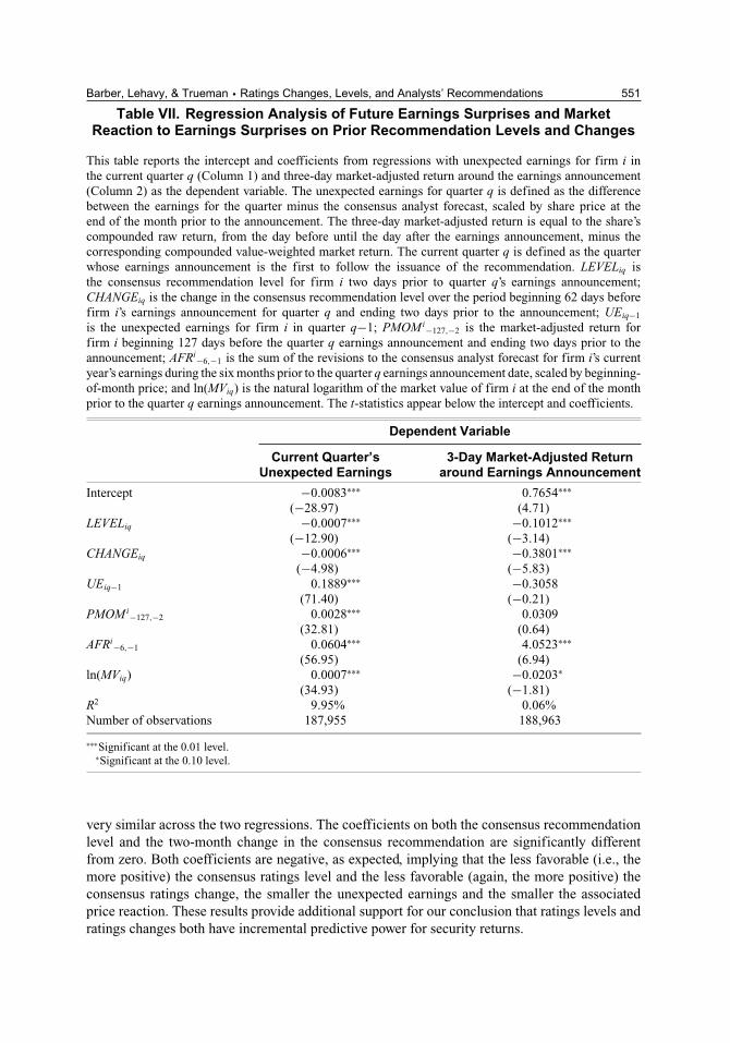
Table VII. Regression Analysis of Future Earnings Surprises and MarketReaction to Earnings Surprises on Prior Recommendation Levels and Changes

This table reports the intercept and coefficients from regressions with unexpected earnings for firm i inthe current quarter q (Column 1) and three-day market-adjusted return around the earnings announcement(Column 2) as the dependent variable. The unexpected earnings for quarter q is defined as the differencebetween the earnings for the quarter minus the consensus analyst forecast, scaled by share price at theend of the month prior to the announcement. The three-day market-adjusted return is equal to the share’scompounded raw return, from the day before until the day after the earnings announcement, minus thecorresponding compounded value-weighted market return. The current quarter q is defined as the quarterwhose earnings announcement is the first to follow the issuance of the recommendation. LEVELiq isthe consensus recommendation level for firm i two days prior to quarter q’s earnings announcement;CHANGEiq is the change in the consensus recommendation level over the period beginning 62 days beforefirm i’s earnings announcement for quarter q and ending two days prior to the announcement; UEiq−1

is the unexpected earnings for firm i in quarter q−1; PMOMi−127,−2 is the market-adjusted return forfirm i beginning 127 days before the quarter q earnings announcement and ending two days prior to theannouncement; AFRi−6,−1 is the sum of the revisions to the consensus analyst forecast for firm i’s currentyear’s earnings during the six months prior to the quarter q earnings announcement date, scaled by beginning-of-month price; and ln(MViq) is the natural logarithm of the market value of firm i at the end of the monthprior to the quarter q earnings announcement. The t-statistics appear below the intercept and coefficients.

Dependent Variable

Current Quarter’s 3-Day Market-Adjusted ReturnUnexpected Earnings around Earnings Announcement

Intercept −0.0083∗∗∗ 0.7654∗∗∗

(−28.97) (4.71)LEVELiq −0.0007∗∗∗ −0.1012∗∗∗

(−12.90) (−3.14)CHANGEiq −0.0006∗∗∗ −0.3801∗∗∗

(−4.98) (−5.83)UEiq−1 0.1889∗∗∗ −0.3058

(71.40) (−0.21)PMOMi−127,−2 0.0028∗∗∗ 0.0309

(32.81) (0.64)AFRi−6,−1 0.0604∗∗∗ 4.0523∗∗∗

(56.95) (6.94)ln(MViq) 0.0007∗∗∗ −0.0203∗

(34.93) (−1.81)R2 9.95% 0.06%Number of observations 187,955 188,963

∗∗∗Significant at the 0.01 level.∗Significant at the 0.10 level.

very similar across the two regressions. The coefficients on both the consensus recommendationlevel and the two-month change in the consensus recommendation are significantly differentfrom zero. Both coefficients are negative, as expected, implying that the less favorable (i.e., themore positive) the consensus ratings level and the less favorable (again, the more positive) theconsensus ratings change, the smaller the unexpected earnings and the smaller the associatedprice reaction. These results provide additional support for our conclusion that ratings levels andratings changes both have incremental predictive power for security returns.


Our findings also yield insights into the mechanism(s) by which ratings levels and changespredict future returns. One possible mechanism is for recommendations to increase the demandfor favorably rated stocks and reduce the demand for unfavorably rated ones, independent ofwhether the recommendations are informative. Another possible (noncompeting) mechanism isfor recommendations to convey to investors analysts’ valuable private information about the futurefinancial success of the firms they cover. Our finding that recommendations have the ability toforecast unexpected earnings and the associated price reaction provides strong evidence that thepredictive power of analysts’ recommendations does not stem solely from their ability to shiftinvestor demand. Rather, it reflects, at least in part, analysts’ skill at gathering relevant privatefinancial information.

VI. Summary and Conclusions

We provide evidence in this paper that the documented abnormal returns to analysts’ recom-mendations are derived from both the ratings levels and the ratings changes. Conditional onratings level, upgrades earn the highest returns and downgrades the lowest. Conditional on thesign and magnitude of a ratings change, the more favorable the recommendation level, the higherthe return.

These results imply that an investment strategy based on both recommendation levels andrecommendation changes has the potential to outperform one based exclusively on one or theother. Conditioning just on recommendation levels, a strategy of purchasing all stocks rated buyor strong buy and shorting all those rated sell or strong sell, for example, would have earnedan average daily abnormal return of 3.5 basis points during our sample period. Conditioningjust on recommendation changes, a strategy of purchasing all stocks receiving a double upgradeand shorting all those receiving a double downgrade would have generated an average dailyabnormal return of 3.8 basis points. However, conditioning on both ratings changes and levelsby purchasing all stocks receiving a double upgrade to buy or strong buy and shorting all thosereceiving a double downgrade to sell or strong sell would have yielded an average daily abnormalreturn of 5.2 basis points. This is a greater than 4 percentage point improvement (on an annualbasis) over the levels-only based strategy and a 3.5% annual improvement over that based solelyon ratings changes.

We also find that ratings levels and changes have the ability to forecast future unexpectedearnings, as well as the corresponding market reactions. In addition to providing further evidencethat the abnormal returns to analysts’ security recommendations are attributable to both levels andchanges, this result implies that the predictive power of analysts’ recommendations is not simplya product of analysts’ ability to shift investor demand; rather, it reflects their skill at collectingvaluable private information about the future financial success of the firms they cover.

As mentioned in the introduction, the formal ratings definitions promulgated by securitiesfirms are fairly uniform: they call for recommendations to be based on analysts’ expectationfor share performance over the recommendation horizon. These expectations are independentof prior ratings level, implying that realized recommendation returns should be independent ofwhether a rating is an upgrade, downgrade, reiteration, or initiation. That ratings changes do haveincremental predictive value for security returns suggests that analysts do not strictly follow thepublished ratings definitions when issuing their recommendations. This conclusion adds to thedebate over whether analysts’ recommendations accurately reflect their investment opinions, anissue that has been of central importance to the SEC in recent years. �


References

Barber, B., R. Lehavy, M. McNichols, and B. Trueman, 2001, “Can Investors Profit from the Prophets?Security Analyst Recommendations and Stock Returns,” Journal of Finance 56, 531-563.

Barber, B., R. Lehavy, M. McNichols, and B. Trueman, 2006, “Buys, Holds, and Sells: The Distribution ofInvestment Banks’ Stock Ratings and the Implications for the Profitability of Analysts’ Recommenda-tions,” Journal of Accounting and Economics 41, 87-117.

Boni, L. and K. Womack, 2002, “Wall Street’s Credibility Problem: Misaligned Incentives and DubiousFixes,” Brookings-Wharton Papers on Financial Services 1, 93-130.

Boni, L. and K. Womack, 2006, “Analysts, Industries, and Price Momentum,” Journal of Financial andQuantitative Analysis 41, 85-109.

Carhart, M., 1997, “On Persistence in Mutual Fund Performance,” Journal of Finance 52, 57-82.

Cliff, M., 2007, “Do Affiliated Analysts Mean What They Say?” Financial Management 36, 1-25.

Green, T.C., 2006, “The Value of Client Access to Analyst Recommendations,” Journal of Financial andQuantitative Analysis 41, 1-24.

Jegadeesh, N. and W. Kim, 2006, “Value of Analyst Recommendations: International Evidence,” Journal ofFinancial Markets 9, 274-309.

Jegadeesh, N., J. Kim, S. Krische, and C. Lee, 2004, “Analyzing the Analysts: When Do RecommendationsAdd Value?,” Journal of Finance 59, 1083-1124.

Jegadeesh, N. and J. Livnat, 2006, “Revenue Surprises and Stock Returns,” Journal of Accounting andEconomics 41, 147-171.

Kadan, O., L. Madureira, R. Wang, and T. Zach, 2009, “Conflicts of Interest and Stock Recommendations:The Effects of the Global Settlement and Related Regulations,” Review of Financial Studies 22, 4189-4217.

Ljungqvist, A., C. Malloy, and F. Marston, 2009, “Rewriting History,” Journal of Finance 64, 1935-1960.

Loh, R. and M. Mian, 2006, “Do Accurate Earnings Forecasts Facilitate Superior Investment Recommen-dations?” Journal of Financial Economics 80, 455-483.

Stickel, S., 1995, “The Anatomy of the Performance of Buy and Sell Recommendations,” Financial AnalystsJournal 51, 25-39.

Womack, K., 1996, “Do Brokerage Analysts’ Recommendations Have Investment Value?” Journal ofFinance 51, 137-167.

Ratings Changes, Ratings Levels, and the Predictive Value of Analysts

Documents

Transcript of Ratings Changes, Ratings Levels, and the Predictive Value of Analysts