Rating Migration and Bond Valuation: Decomposing...

Expert Journal of Finance, Volume 5, pp.49-72, 2017

© 2017 The Author. Published by Sprint Investify. ISSN 2359-7712

http://Finance.ExpertJournals.com

49

Rating Migration and Bond Valuation:

Decomposing Rating Migration Matrices from

Market Data via Default Probability

Term Structures

Brian BARNARD*

University of Johannesburg, South Africa

The study builds on previous research that decomposes rating category default

probability term structures from rating category interest rate term structures, and

proposes a method to decompose rating migration matrices from market data, via

decomposed default probability term structures. To investigate the power and

accuracy of the proposed method, it was examined to what extent an existing, known

rating migration matrix could again be surfaced by the method. Overall, the results

are more than satisfactory, and the method promises to be accurate. Although not

considered here, the main objective is the application of the method to market data.

The outcome should be insightful in itself, and can be used to evaluate historical

rating migration matrices commonly devised by rating agencies, and to form a better

understanding of the default probability term structures embedded in market data.

Keywords: Default Probability, Default Risk, Credit Risk, Rating Migration, Bond

Valuation, Optimization

JEL Classification: G32, G12

1. Introduction

1.1. The Factors Impacting Bond Valuation

The extent by which credit risk explain bond premiums is a predominant topic in bond valuation

research. A number of authors conclude that it only accounts for a small fraction of bond premiums (Huang

and Huang, 2012; Geske and Delianedis, 2001; Elton et al, 2001).

The predominant factors affecting bond prices are listed as risk free rates, taxes, jumps, liquidity,

*Corresponding Author:

Brian Barnard, Wits Business School, University of Johannesburg, Johannesburg, South Africa

Article History:

Received 23 May 2017 | Accepted 13 September 2017 | Available Online 23 September 2017

Cite Reference:

Barnard, B., 2017. Rating Migration and Bond Valuation: Decomposing Rating Migration Matrices from Market Data via Default Probability Term

Structures. Expert Journal of Finance, 5, pp. 49-72.

Acknowledgment:

The Author would like to thank PolyComp (Pty) Ltd for a grant received for the paper.



50

market risk factors, issue traits, equity volatility, market risk, systematic risk, and macroeconomic risk factors

(Houweling et al, 2005; Geske and Delianedis, 2001; Elton et al, 2004; Elton et al, 2001; Grandes and Peter,

2005; Delianedis and Geske, 2003; Campbell and Taksler, 2003; Collin‐Dufresne et al 2001; Athanassakos

and Carayannopoulos, 2001; Fama and French, 1993; Merton, 1974).

A number of studies also look at credit rating migration risk, or simply credit migration risk. Das and

Tufano (1995) state investors are exposed to three risks: interest rate risk, changes in credit risk caused by

changes in the credit rating of the issuer of the debt, and changes in credit risk caused by changes in spreads

on the debt, even when ratings have not changed. Altman (1996) examines the expected spread change and

cost implication due to credit rating migration. In the context of portfolios, Fei et al (2012) note that risk models

generally predict for each asset in the portfolio, the corresponding probability of default (PD), exposure at

default (EAD) and loss given default (LGD). Similarly, Kadam and Lenk (2008) note different estimates for

risk capital, derived from loss distributions, which they quantify as Value-at-Risk (VAR) and Expected Loss

(EL) for the portfolio at hand. Jarrow et al (1997) models the impact in forward rates – and thus bond value –

due to credit rating jumps.

Delianedis and Geske (2003) note that default probabilities and changes in expected default

frequencies are important to both the structure and pricing of credit derivatives. All corporate issuers have

some positive probability of default. This default probability should change continuously with changes in the

firm’s stock price and thus its leverage. The value of most fixed income securities is typically inversely related

to the probability of default. Investors are concerned about changes in the value of their fixed income securities

due to changes in the probability of default, even though the actual default seldom occurs. In fact, fixed income

investors may be more concerned with changes in the perceived credit quality of their bond holdings than with

actual default. Rating migrations, which offer one reflection of changes in perceived quality of bonds, occur

much more frequently than defaults.

Foss (1995) specifically differentiates between credit risk and default risk. He notes that the terms

default risk and credit risk are often used interchangeably; however, they are not one and the same. Default

risk is defined as the risk that the issuer of a fixed-income security will be unable to make timely payments of

interest or principal. This risk, diversified over a portfolio of equally rated securities, leads to an expected

default loss. Many of the initial studies on risks and returns focus on historical default rates and losses.

Although these studies provide valuable insight, default rates and default losses, in isolation, are not

paramount. Credit risk is defined as the risk that the perceived credit quality of an issuer will change, although

default is not necessarily a certain event. Increased credit risk is reflected in a widening of the yield spread.

Credit and default risk are correlated because credit deterioration is almost always a precursor to eventual

default; even in the most drastic cases, however, until default actually occurs, the potential for recovery or

stabilization cannot be totally discounted. In line with this, Manzoni (2004) makes the point that, while several

studies model default and bankruptcy events, no empirical work directly models the probability of a bond

having its rating revised. He points out the traditional default mode of thinking of most financial institutions,

leading to a consensus view of transitions as non-fundamental economic events.

1.2. Credit Default Swaps and Bond Valuation

Norden and Weber (2009) argue that CDS should reflect pure issuer default risk, and no facility or

issue specific risk, making these instruments a potentially ideal benchmark for measuring and pricing credit

risk. According to Blanco et al (2005), CDSs are an upper bound on the price of credit risk (while credit spreads

form a lower bound). Benkert (2004) argues that CDS premia represent primarily a price of default risk, and

are in this respect similar to bond spreads. Consequently, CDS premia and bond spreads should be driven by

the same factors. A number of studies (Benkert, 2004; Ericsson et al, 2009) indeed consider the same factors

of bond valuation to explain CDS premiums. Weistroffer et al (2009) mention that rating agencies use

information derived from CDS prices to calculate market implied ratings.

1.3. Default Probability

Zhu (2006) states that, in general, measures of credit risk consist of three building blocks: probability

of default (PD), loss given default (LGD) and correlation between PD and LGD. In order to model default risk,

Athanassakos and Carayannopoulos (2001), consider three proxy variables: i) credit rating, which captures the

effect of both the probability of default and the recovery rate; ii) time to maturity; iii) the existence of a sinking

fund. Both of the latter two proxies should be related to the probability of default.

Grandes and Peter (2005) note that, when government bonds are not truly risk-free, particularly in an

emerging market, the corporate yield spread above an equivalent government bond yield does not reflect

corporate default risk, even after controlling for all other factors. It merely reflects corporate default risk in



51

excess of sovereign default risk. They model corporate default probability as the probability that the firm

defaults given that the sovereign does not default, plus the probability that the firm defaults given that the

sovereign has defaulted.

Campbell and Taksler (2003) note that the literature distinguishes between structural and reduced form

models. The authors note that “In structural models, a firm is assumed to default when the value of its liabilities

exceeds the value of its assets, in which case bondholders assume control of the company in exchange for its

residual value. Reduced form models, by contrast, assume exogenous stochastic processes for the default

probability and the recovery rate. The added flexibility of the reduced-form approach allows default risk to

play a somewhat greater role in the pricing of corporate bonds.”

Merton (1974) shows that for a given maturity, the risk of default varies directly with the variance of

the returns on the firm value. In this context, the business cycle and economic environment impact both the

level of the risk free rate and the variance of returns on the firm value.

Huang and Huang (2012) consider a credit risk model with a counter-cyclical market risk premium to

capture the effects of business cycles on credit risk premia. Secondly, they introduce an analytically tractable

jump-diffusion structural credit risk model to capture the effects on credit risk premia of certain future states

with both high default risks and abnormally high stochastic discount factors. The second mechanism is

distinctly different from the first mechanism. In the model with jumps in asset values, the jumps are

unpredictable and there is no time variation in market risk premia.

In line with reduced form models, Elton et al (2001) develop marginal default probabilities from a

rating transition matrix employing the assumption that the rating transition process is stationary and

Markovian. In year one, the marginal probability of default can be determined directly from the transition

matrix and default vector, and is, for each rating class, the proportion of defaults in year one. To obtain

subsequent year defaults, they first use the transition matrix to calculate the ratings going into a given year for

any bond starting with a particular rating in the previous year. The defaults of that year are then the proportion

in each rating class multiplied by the probability that a bond in that class defaults by year end. They find that

the marginal probability of default increases for the high-rated debt and decreases for the low-rated debt. This

occurs because bonds change rating classes over time.

A number of studies use bond valuation models – both structural and reduced form – to note the extent

by which market prices can be modelled, and to note the magnitude of default probability as bond valuation

factor (Eom et al, 2004; Elton et al, 2001; Huang and Huang, 2012; Geske and Delianedis, 2001; Collin‐Dufresne et al, 2001).

Fei et al (2012) note a credit rating is a financial indicator of an obligor’s level of creditworthiness.

Given the relationship between credit ratings and default probability or credit quality, Kumar and Haynes

(2003) discuss rating methodology and list the key factors considered as: i) business analysis (industry risk;

market position; operating efficiency; legal position), ii) financial analysis (accounting quality; earnings

protection; adequacy of cash flows; financial flexibility; interest and tax sensitivity), and iii) management

evaluation (track record of management; evaluation of capacity to overcome adverse situations; goals,

philosophy and strategies). They find that financial parameters reflect, to a significant extent, the subjective

and objective factors used by an expert while rating a debt obligation, with hidden relationships between the

financial parameters and associated expert rating.

A number of authors examine the timeliness, accuracy and actual information content of credit rating

agencies' ratings (Hines et al, 1975; Ederington and Goh, 1998; Amato and Furfine, 2004). Amato and Furfine

(2004) mention that rating agencies insist that their ratings should be interpreted as ordinal rankings of default

risk that are valid at all points in time, rather than absolute measures of default probability that are constant

through time. Delianedis and Geske (2003) note that rating agencies regularly measure the historical default

frequency of corporate issuers. While these historical default frequencies are interesting, they are not forward-

looking. Option models can provide a forward-looking, risk neutral default probability. Chan and Jegadeesh

(2004) point to evidence that agency ratings may not be accurate in a timely fashion.

Studies like Wang (2004) attempt to model default ratings, and studies like Hines et al (1975), Kaplan

and Urwitz (1979), Belkaoui (1980) and Chan and Jegadeesh (2004) statistically model bond ratings. This

may provide alternative default probability estimates, as structural models also do, relative to the credit ratings

of credit rating agencies, but must still be translated to default probability term structures, in a similar way

credit agencies' ratings are translated.

Also, a number of studies quantify credit ratings as proxies of credit quality in terms of spread (Foss,

1995; Kaplan and Urwitz, 1979; Cantor et al, 1997; Perraudin and Taylor, 2004; Chan and Jegadeesh, 2004).



52

1.4. Default Probability Term Structures

Altman (1989) notes that analysts have concentrated their efforts on measuring the default rate for

finite periods of time – for example, one year – and then averaging the annual rates for longer periods.

Elton (1999) argues that realized returns are a very poor measure of expected returns and that

information surprises highly influence a number of factors in an asset pricing model. He believes that

developing better measures of expected return and alternative ways of testing asset pricing theories that do not

require using realized returns have a much higher payoff than any additional development of statistical tests

that continue to rely on realized returns as a proxy for expected returns. He argues that either there are

information surprises that are so large or that a sequence of these surprises is correlated so that the cumulative

effect is so large that they have a significant permanent effect on the realized mean. Furthermore, these

surprises can dominate the estimate of mean returns and be sufficiently large that they are still a dominant

influence as the observation interval increases. Thus, the difference between expected and realized returns is

viewed as a mixture of two distributions, one with standard properties and the other that more closely resembles

a jump process.

Duffie and Singleton (1999) state that, because of the possibility of sudden changes in perceptions of

credit quality, particularly among low-quality issues such as Brady bonds, one may wish to allow for surprise

jumps in default probability.

Nelson and Siegel (1987) state the range of shapes generally associated with interest rate term

structures: monotonic, humped, and S shaped. Related to this, a number of studies consider the relationship or

correlation between default probability, interest rates, and the state of the economy (Benkert, 2004; Duffie and

Singleton, 1999; Das and Tufano, 1995; Huang and Huang, 2012; Athanassakos and Carayannopoulos, 2001;

Amato and Furfine, 2004; Delianedis and Geske, 2003; Longstaff and Schwartz, 1995; Kim et al 1993;

Campbell and Taksler, 2003; Lando and Skødeberg, 2002; Hamilton and Cantor, 2004).

Benkert (2004) argue that corporate defaults occur more often during economic downturns than during

boom phases, and the occurrence of a recession may cause a decline in credit quality that leads to more defaults

in the future. According to this line of reasoning, the compensation for default risk would rise. Duffie and

Singleton (1999) note strong evidence that hazard rates for default of corporate bonds vary with the business

cycle. Equally, recovery data also exhibit a pronounced cyclical component. Das and Tufano (1995) allowed

recovery to vary over time so as to induce a non-zero correlation between credit spreads and the riskless term

structure. However, for computational tractability they maintained the assumption of independence of the

hazard rate (default rate) and risk-free rate.

Huang and Huang (2012) argue that a credit risk premium is required by investors because the

uncertainty of default loss should be systematic – bondholders are more likely to suffer default losses in bad

states of the economy. Moreover, precisely because of the tendency for default events to cluster in the worst

states of the economy, the credit risk premium can be potentially very large. Athanassakos and

Carayannopoulos (2001) note that yield spreads are greater during recessions than during recoveries, and also

point to the link between the behaviour of yield spreads to the shape of the term structure, as a proxy of the

business cycle. They confirm the typical direct relationship between default risk and yield spreads, and show

that the impact of the business cycle (macro-economy) on the yield spread of a corporate bond depends on the

industry sector to which the issuer of the bond belongs. The inflation rate should be directly related to yield

spreads, since during inflationary periods investors may require higher risk premia from their investments in

corporate bonds.

Athanassakos and Carayannopoulos (2001) use the change in the shape of the term structure of interest

rates – represented by the quarterly change in the difference between the 20-year treasury rates and the three

month t-bill rates – as a proxy for the business cycle, since much research in the past has linked the shape of

the treasury term structure to future variations in the business cycle. A steepening term structure is a typical

result of robust economic growth and lower short term interest rates and reflects a general belief in a more

robust economic future. The opposite is true when the term structure is flattening or turns negatively sloped.

Therefore, the particular proxy should be negatively related to yield spreads. Finally, the annual rate of change

in the industrial production index should be negatively related to yield spreads since increased economic

activity will bolster investors’ confidence in the corporate sector, and lead to a reduction in the risk premia

demanded for investment in corporate bonds.

Amato and Furfine (2004) argue that financial market participants behave as if risk is countercyclical,

e.g. at its highest during economic downturns. Empirical models, too, tend to indicate a rise in risk during

recessions. There is a relationship between the correlation of default rates and loss in the event of default and

the business cycle. Models that assume independence of default probabilities and loss given default will tend

to underestimate the probability of severe losses during economic downturns. They delineate the empirical



53

significance of the pro-cyclicality of credit quality changes by showing that estimated credit losses are much

higher in a contraction relative to an expansion.

Longstaff and Schwartz (1995) argue that the corporate yield spread should vary inversely with the

benchmark treasury yield, and find evidence to support this. Kim et al (1993) show that default risk is not

particularly sensitive to the volatility of interest rates but is sensitive to interest rate expectations. Campbell

and Taksler (2003) note idiosyncratic volatility can move very differently from market-wide volatility.

Movements in idiosyncratic risk are more persistent than movements in market risk. Lando and Skødeberg

(2002) note that it is likely that macroeconomic variables or other indicators of the business cycle influence

rating intensities.

A number of studies model default probability term structures as instantaneous stochastic processes

(Das and Tufano, 1995; Duffee, 1999; Jarrow et al, 2002) . For example, Duffee (1999) uses the extended

Kalman filter to fit yields on bonds issued by individual investment-grade firms to a model of instantaneous

default risk. Das and Tufano (1995) and Jarrow et al (1997) model default risk as Markov chains or trees.

Jarrow and Turnbull (1995) exogenously specify a stochastic process for the evolution of the default-free term

structure and the term structure for risky debt.

Duffee (1999) argues that at each instant there is some probability that a firm defaults on its

obligations. Both this probability and the recovery rate in the event of default may vary stochastically through

time. The stochastic processes determine the price of the credit risk. Although these processes are not formally

linked to an organization’s asset value, it can be assumed there is some underlying relation. The instantaneous

probability that a given firm defaults on its obligated bond payments follow a translated single-factor square-

root diffusion process, with a modification that allows the default process to be correlated with the factors

driving the default-free term structure. There are a number of factors other than default risk that drive a

discrepancy between corporate and Treasury bond prices, such as liquidity differences, state taxes, and special

repo rates. Here, all of these factors are substituted into a stochastic process called a default risk process.

Default risk is negatively correlated with the default-free interest rates. For a typical firm, the instantaneous

risk of default has a lower bound that exceeds zero. In other words, even if an organization’s financial health

dramatically improves, the model implies that yield spreads on the organization’s bonds remain positive.

Duffee (1999) first models the price of a risk-free bond as given by the expectation, under the

equivalent martingale measure, of the cumulative discount rate between t and T. The discount rate follows a

stochastic process – the sum of a constant, and two factors that follow independent square-root stochastic

processes. He then models the adjusted discount rate for bond issues that can default, relative to risk-free

bonds. This setup is designed to capture three important empirical features of corporate bond yield spreads.

The most obvious is that the spreads are stochastic, fluctuating with the financial health of the firm. The second

feature is that yield spreads for very high-quality firms are positive, even at the short end of the yield curve.

This fact suggests that regardless of how healthy a firm may seem, there is some level below which yield

spreads cannot fall. The third feature is that yield spreads, especially spreads for lower quality bonds, appear

to be systematically related to variations in the default-free term structure.

Houweling and Vorst (2005) note reduced form models that use time series estimation to model the

hazard rate stochastically, typically as a Vasicek or CIR process. Also, other reduced form models use cross-

sectional estimation and consider either constant or stochastic hazard rates, where the stochastic process is

chosen in such a way that the survival probability curve is known analytically. Houweling and Vorst (2005)

follow an intermediate approach by using a deterministic function of time to maturity. This specification

facilitates parameter estimation, while still allowing for time-dependency. They model the integrated hazard

function as a polynomial function of time to maturity, with three degrees – linear, quadratic and cubic.

Das and Tufano (1995) choose to make recovery rates correlated with the term structure of interest

rates. This results in a model wherein credit spreads are correlated with interest rates, as is evidenced in

practice. In the Jarrow-Lando-Turnbull model credit spreads change only when credit ratings change, whereas

in the debt markets it is found that credit spreads change even when ratings have not changed. Injecting

stochastic recovery rates into the model provides this extra feature.

In the context of default probability term structures, credit migration and credit migration matrices

should also be mentioned.

A number of studies examine the stochastic processes associated with rating transitions (Frydman and

Schuermann, 2008; Lando and Skødeberg, 2002; Hamilton and Cantor, 2004; Altman, 1996). Altman and

Rijken (2004) investigate the through-the-cycle methodology that agencies use, in the context of bond

valuation, and rating timeliness and rating stability.

Nickell et al (2000) use Moody’s data from 1970 to 1997 to examine the dependence of ratings

transition probabilities on industry, country and stage of the business cycle using an ordered probit approach,



54

and they find that the “business cycle dimension is the most important in explaining variation of these transition

probabilities”. They point out that rating transition matrices vary according to the stage of the business cycle,

the industry of the obligor and the length of time that has elapsed since the issuance of the bond. Kadam and

Lenk (2008) identified strong differences in rating migration behaviour between issuers of different industry

sectors and countries.

Bangia et al (2002) argue that “credit migration matrices provide specific linkage between underlying

macroeconomic conditions and asset quality”. Credit migration matrices characterize the expected changes in

credit quality of obligors. Total volatility (risk) is composed of a systematic and an idiosyncratic component.

Because ratings are a reflection of a firm’s asset quality and distance to default, a reasonable definition of

“systematic” is the state of the economy. They find distinct differences between the U.S. expansion and

contraction transition matrices. The most striking difference between expansion and contraction matrices are

the downgrading and especially the default probabilities that increase significantly in contractions. Overall,

these results reveal that migration probabilities are more stable in contractions than they are on average,

supporting the existence of two distinct economic regimes. The rating universe should develop differently in

contraction periods compared to expansion times.

The straightforward application of these matrices however would normally be restricted to situations

where the future state of the economy over the transition horizon under consideration is assumed to be known.

The condition of the economy unmistakably is one of the real drivers of systematic credit risk, especially as

lower credit classes are substantially more delicate to macro-economic factors. Consequently it ought to be

integrated into credit risk modelling whenever possible, otherwise the downward potential of high-yield

portfolios in contractions might be underestimated. Modern credit risk models represent different industries

only through different term structures, yet not through industry dependent transition matrices.

Fei et al (2012) proposes an approach to estimate credit rating migration risk that controls for the

business-cycle evolution during the relevant time horizon in order to ensure adequate capital buffers both in

good and bad times. The approach allows the default risk associated with a given credit rating to change as the

economy moves through different points in the business cycle. They mention a body of research linking

portfolio credit risk with macroeconomic factors showing, for instance, that default risk tends to increase

during economic downturns. Their premise is that point-in-time methodologies that account for business cycles

should provide more realistic credit risk measures than through-the-cycle models that smooth out transitory

fluctuations (perceived as random noise) in economic fundamentals.

1.5. Decomposing Default Probabilities from Market Data

1.5.1. Decomposing Rating Migration Matrices from Market Data

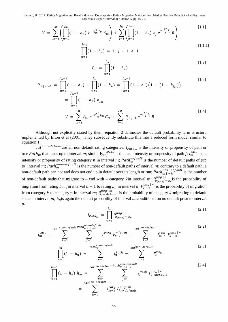
Taken from Barnard (2017a), equation 1 states the reduced form model of Duffie and Singleton (1999),

adapted for coupon paying bonds. Equation 1 has two components, a coupon paying component associated

with non-default outcomes, and a recovery component associated with default outcomes.

In the equation, 𝑉 is the price or value of the risk-bearing bond; 𝑀is the number of coupons of the

bond, including par; 𝐶𝑚is the coupon of the bond on coupon date 𝑚; 𝑅is the recovery of par value; 𝑟𝑡𝑚

𝑟𝑓 and

𝑡𝑚 are the risk-free spot rate and time value, respectively, associated with coupon date 𝑚; ℎ𝑛is the default

probability of interval 𝑛, conditional on no default prior to interval 𝑛; 𝑃𝑚is the cumulative non-default

probability of interval 𝑚; 𝐽𝑚 is the number of probability intervals for which the possibility of default is

considered up to coupon date 𝑚; 𝐽𝑀 is the number of probability intervals considered up to maturity.

For coupon paying bonds, it is convenient to consider 𝐽𝑚 and 𝐽𝑀 to be equal to 𝑚 and 𝑀. For example,

the third coupon may have three probability intervals leading up to it. For zero-coupon bonds, 𝑀 is equal to 1,

and 𝐽𝑀 may be greater than 𝑀, with 𝐽𝑚 not necessarily corresponding with 𝑚; a regular coupon interval may

still be considered though to ensure a timely and consistent consideration of default. A five-year zero coupon

bond will have only one coupon, but can have up to ten probability intervals leading up to it, if semi-annual

probability intervals are used.



55

𝑉 = ∑ (∏(1 − ℎ𝑛)

𝐽𝑚

𝑛=1

𝑒−𝑟𝑡𝑚

𝑟𝑓 𝑡𝑚 𝐶𝑚)

𝑀

𝑚=1

+ ∑ (∏(1 − ℎ𝑛)

𝑗−1

𝑛=1

ℎ𝑗 𝑒−𝑟𝑡𝑗

𝑟𝑓 𝑡𝑗

𝑅)

𝐽𝑀

𝑗=1

[1.1]

∏(1 − ℎ𝑛)

𝑗−1

𝑛=1

= 1 ; 𝑗 − 1 < 1

[1.1.1]

𝑃𝑚 = ∏(1 − ℎ𝑛)

𝐽𝑚

𝑛=1

[1.2]

𝑃𝑚 | 𝑚−1 = ∏ (1 − ℎ𝑛)

𝐽𝑚−1

𝑛=1

− ∏(1 − ℎ𝑛)

𝐽𝑚

𝑛=1

= ∏ (1 − ℎ𝑛)

𝐽𝑚−1

𝑛=1

(1 − (1 − ℎ𝐽𝑚))

= ∏ (1 − ℎ𝑛)

𝐽𝑚−1

𝑛=1

ℎ𝐽𝑚

[1.3]

𝑉 = ∑ 𝑃𝑚

𝑀

𝑚=1

𝑒−𝑟𝑡𝑚

𝑟𝑓 𝑡𝑚 𝐶𝑚 + ∑

𝐽𝑀

𝑗=1

𝑃𝑗 | 𝑗−1 𝑒−𝑟𝑡𝑗

𝑟𝑓 𝑡𝑗

𝑅

[1.4]

Although not explicitly stated by them, equation 2 delineates the default probability term structure

implemented by Elton et al (2001). They subsequently substitute this into a reduced form model similar to

equation 1.

𝑐𝑎𝑡𝑛𝑜𝑛−𝑑𝑒𝑓𝑎𝑢𝑙𝑡are all non-default rating categories; 𝐼𝑃𝑎𝑡ℎ𝑚 is the intensity or propensity of path or

tree 𝑃𝑎𝑡ℎ𝑚 that leads up to interval 𝑚; similarly, 𝐼𝑗𝑃𝑎𝑡ℎ is the path intensity or propensity of path 𝑗; 𝐼𝑚

𝑐𝑎𝑡𝑛is the

intensity or propensity of rating category 𝑛 in interval 𝑚; 𝑃𝑎𝑡ℎ𝑚𝑑𝑒𝑓𝑎𝑢𝑙𝑡

is the number of default paths of (up

to) interval 𝑚; 𝑃𝑎𝑡ℎ𝑚𝑛𝑜𝑛−𝑑𝑒𝑓𝑎𝑢𝑙𝑡

is the number of non-default paths of interval 𝑚; contrary to a default path, a

non-default path can not and does not end up in default over its length or run; 𝑃𝑎𝑡ℎ𝑚 | → 𝑘𝑛𝑜𝑛−𝑑𝑒𝑓𝑎𝑢𝑙𝑡

is the number

of non-default paths that migrate to – end with – category 𝑘in interval 𝑚; 𝑃𝑏(𝑛−1) → 𝑏𝑛

𝑚𝑖𝑔 | 𝑛is the probability of

migration from rating 𝑏𝑛−1in interval 𝑛 − 1 to rating 𝑏𝑛 in interval 𝑛; 𝑃𝑘 → 𝑛𝑚𝑖𝑔 | 𝑚

is the probability of migration

from category 𝑘 to category 𝑛 in interval 𝑚; 𝑃𝑘 → 𝑑𝑒𝑓𝑎𝑢𝑙𝑡𝑚𝑖𝑔 | 𝑚

is the probability of category 𝑘 migrating to default

status in interval 𝑚; ℎ𝑛is again the default probability of interval 𝑛, conditional on no default prior to interval

𝑛.

𝐼𝑃𝑎𝑡ℎ𝑚 = ∏ 𝑃𝑏(𝑛−1) → 𝑏𝑛

𝑚𝑖𝑔 | 𝑛

𝐽𝑚

𝑛=1

[2.1]

𝐼𝑚𝑐𝑎𝑡𝑛 = ∑ ∑ 𝐼𝑗

𝑃𝑎𝑡ℎ

𝑃𝑎𝑡ℎ𝑚−1 | → 𝑘𝑛𝑜𝑛−𝑑𝑒𝑓𝑎𝑢𝑙𝑡

𝑗=1

𝑐𝑎𝑡𝑛𝑜𝑛−𝑑𝑒𝑓𝑎𝑢𝑙𝑡

𝑘=1

𝑃𝑘 → 𝑛𝑚𝑖𝑔 | 𝑚

= ∑ 𝐼𝑚−1𝑐𝑎𝑡𝑘


𝑘=1

𝑃𝑘 → 𝑛𝑚𝑖𝑔 | 𝑚

[2.2]

∏(1 − ℎ𝑛)

𝑚

𝑛=1

= ∑ 𝐼𝑛𝑃𝑎𝑡ℎ

𝑃𝑎𝑡ℎ𝑚𝑛𝑜𝑛−𝑑𝑒𝑓𝑎𝑢𝑙𝑡

𝑛=1

= ∑ 𝐼𝑚𝑐𝑎𝑡𝑛


𝑛=1

[2.3]

∏(1 − ℎ𝑛)

𝑚−1

𝑛=1

ℎ𝑚 = ∑ ∑ 𝐼𝑗𝑃𝑎𝑡ℎ

𝑃𝑎𝑡ℎ𝑚−1 | →𝑘𝑛𝑜𝑛−𝑑𝑒𝑓𝑎𝑢𝑙𝑡

𝑗=1


𝑘=1

𝑃𝑘→𝑑𝑒𝑓𝑎𝑢𝑙𝑡𝑚𝑖𝑔 | 𝑚

= ∑ 𝐼𝑚−1𝑐𝑎𝑡𝑘


𝑘=1

𝑃𝑘 → 𝑑𝑒𝑓𝑎𝑢𝑙𝑡𝑚𝑖𝑔 | 𝑚

[2.4]



56

ℎ𝑛 = 1 − (∏(1 − ℎ𝑚)

𝑛

𝑚=1

⁄ ∏(1 − ℎ𝑚)

𝑛−1

𝑚=1

)

= ( ∑


𝑘=1

𝐼𝑛−1𝑐𝑎𝑡𝑘 𝑃𝑘 → 𝑑𝑒𝑓𝑎𝑢𝑙𝑡

𝑚𝑖𝑔 | 𝑛) ⁄ (∏(1 − ℎ𝑚)

𝑛−1

𝑚=1

)

[2.5]

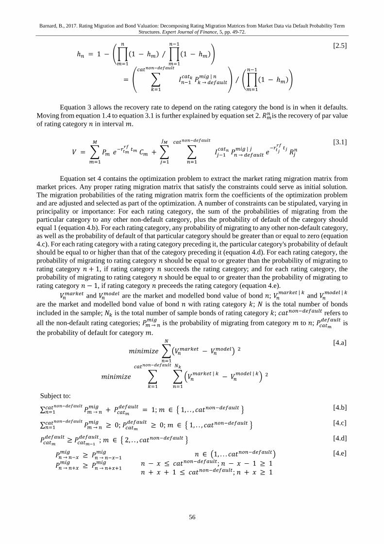
Equation 3 allows the recovery rate to depend on the rating category the bond is in when it defaults.

Moving from equation 1.4 to equation 3.1 is further explained by equation set 2. 𝑅𝑚𝑛 is the recovery of par value

of rating category 𝑛 in interval 𝑚.

𝑉 = ∑ 𝑃𝑚

𝑀

𝑚=1

𝑒−𝑟𝑡𝑚

𝑟𝑓 𝑡𝑚 𝐶𝑚 + ∑

𝐽𝑀

𝑗=1

∑


𝑛=1

𝐼𝑗−1𝑐𝑎𝑡𝑛 𝑃𝑛 → 𝑑𝑒𝑓𝑎𝑢𝑙𝑡

𝑚𝑖𝑔 | 𝑗 𝑒

−𝑟𝑡𝑗

𝑟𝑓 𝑡𝑗

𝑅𝑗𝑛

[3.1]

Equation set 4 contains the optimization problem to extract the market rating migration matrix from

market prices. Any proper rating migration matrix that satisfy the constraints could serve as initial solution.

The migration probabilities of the rating migration matrix form the coefficients of the optimization problem

and are adjusted and selected as part of the optimization. A number of constraints can be stipulated, varying in

principality or importance: For each rating category, the sum of the probabilities of migrating from the

particular category to any other non-default category, plus the probability of default of the category should

equal 1 (equation 4.b). For each rating category, any probability of migrating to any other non-default category,

as well as the probability of default of that particular category should be greater than or equal to zero (equation

4.c). For each rating category with a rating category preceding it, the particular category's probability of default

should be equal to or higher than that of the category preceding it (equation 4.d). For each rating category, the

probability of migrating to rating category 𝑛 should be equal to or greater than the probability of migrating to

rating category 𝑛 + 1, if rating category 𝑛 succeeds the rating category; and for each rating category, the

probability of migrating to rating category 𝑛 should be equal to or greater than the probability of migrating to

rating category 𝑛 − 1, if rating category 𝑛 preceeds the rating category (equation 4.e).

𝑉𝑛𝑚𝑎𝑟𝑘𝑒𝑡 and 𝑉𝑛

𝑚𝑜𝑑𝑒𝑙 are the market and modelled bond value of bond 𝑛; 𝑉𝑛𝑚𝑎𝑟𝑘𝑒𝑡 | 𝑘

and 𝑉𝑛𝑚𝑜𝑑𝑒𝑙 | 𝑘

are the market and modelled bond value of bond 𝑛 with rating category 𝑘; 𝑁 is the total number of bonds

included in the sample; 𝑁𝑘 is the total number of sample bonds of rating category 𝑘; 𝑐𝑎𝑡𝑛𝑜𝑛−𝑑𝑒𝑓𝑎𝑢𝑙𝑡 refers to

all the non-default rating categories; 𝑃𝑚 → 𝑛𝑚𝑖𝑔

is the probability of migrating from category 𝑚 to 𝑛; 𝑃𝑐𝑎𝑡𝑚

𝑑𝑒𝑓𝑎𝑢𝑙𝑡 is

the probability of default for category 𝑚.

𝑚𝑖𝑛𝑖𝑚𝑖𝑧𝑒 ∑(𝑉𝑛𝑚𝑎𝑟𝑘𝑒𝑡 − 𝑉𝑛

𝑚𝑜𝑑𝑒𝑙)

𝑁

𝑛=1

2

𝑚𝑖𝑛𝑖𝑚𝑖𝑧𝑒 ∑ ∑ (𝑉𝑛𝑚𝑎𝑟𝑘𝑒𝑡 | 𝑘

− 𝑉𝑛𝑚𝑜𝑑𝑒𝑙 | 𝑘

)

𝑁𝑘

𝑛=1


𝑘=1

2

[4.a]

Subject to:

∑ 𝑃𝑚 → 𝑛𝑚𝑖𝑔𝑐𝑎𝑡𝑛𝑜𝑛−𝑑𝑒𝑓𝑎𝑢𝑙𝑡

𝑛=1 + 𝑃𝑐𝑎𝑡𝑚

𝑑𝑒𝑓𝑎𝑢𝑙𝑡 = 1; 𝑚 ∈ { 1, . . , 𝑐𝑎𝑡𝑛𝑜𝑛−𝑑𝑒𝑓𝑎𝑢𝑙𝑡 } [4.b]


𝑛=1 ≥ 0; 𝑃𝑐𝑎𝑡𝑚

𝑑𝑒𝑓𝑎𝑢𝑙𝑡 ≥ 0; 𝑚 ∈ { 1, . . , 𝑐𝑎𝑡𝑛𝑜𝑛−𝑑𝑒𝑓𝑎𝑢𝑙𝑡 } [4.c]

𝑃𝑐𝑎𝑡𝑚

𝑑𝑒𝑓𝑎𝑢𝑙𝑡≥ 𝑃𝑐𝑎𝑡𝑚−1

𝑑𝑒𝑓𝑎𝑢𝑙𝑡; 𝑚 ∈ { 2, . . , 𝑐𝑎𝑡𝑛𝑜𝑛−𝑑𝑒𝑓𝑎𝑢𝑙𝑡 } [4.d]

𝑃𝑛 → 𝑛−𝑥𝑚𝑖𝑔

≥ 𝑃𝑛 → 𝑛−𝑥−1𝑚𝑖𝑔

𝑃𝑛 → 𝑛+𝑥𝑚𝑖𝑔

≥ 𝑃𝑛 → 𝑛+𝑥+1𝑚𝑖𝑔

𝑛 ∈ (1, . . . 𝑐𝑎𝑡𝑛𝑜𝑛−𝑑𝑒𝑓𝑎𝑢𝑙𝑡)

𝑛 − 𝑥 ≤ 𝑐𝑎𝑡𝑛𝑜𝑛−𝑑𝑒𝑓𝑎𝑢𝑙𝑡; 𝑛 − 𝑥 − 1 ≥ 1

𝑛 + 𝑥 + 1 ≤ 𝑐𝑎𝑡𝑛𝑜𝑛−𝑑𝑒𝑓𝑎𝑢𝑙𝑡; 𝑛 + 𝑥 ≥ 1

[4.e]



57

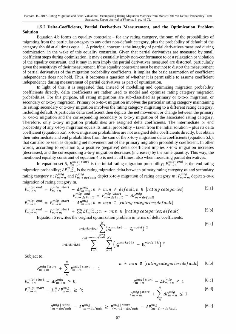
1.5.2. Delta-Coefficients, Partial Derivatives Measurement, and the Optimization Problem

Solution

Equation 4.b forms an equality constraint – for any rating category, the sum of the probabilities of

migrating from the particular category to any other non-default category, plus the probability of default of the

category should at all times equal 1. A principal concern is the integrity of partial derivatives measured during

optimization, in the wake of this equality constraint. Given that partial derivatives are measured by small

coefficient steps during optimization, it may essentially imply non-conformance to or a relaxation or violation

of the equality constraint, and it may in turn imply the partial derivatives measured are distorted, particularly

given the sensitivity of their measurement. If the equality constraint must be met not to distort the measurement

of partial derivatives of the migration probability coefficients, it implies the basic assumption of coefficient

independence does not hold. Thus, it becomes a question of whether it is permissible to assume coefficient

independence during measurement of partial derivatives as part of optimization.

In light of this, it is suggested that, instead of modelling and optimizing migration probability

coefficients directly, delta coefficients are rather used to model and optimize rating category migration

probabilities. For this purpose, all rating migrations are sub-classified as primary or x-to-x migration, or

secondary or x-to-y migration. Primary or x-to-x migration involves the particular rating category maintaining

its rating; secondary or x-to-y migration involves the rating category migrating to a different rating category,

including default. A particular delta coefficient then depicts the net movement or change between the primary

or x-to-x migration and the corresponding secondary or x-to-y migration of the associated rating category.

Therefore, only x-to-y migration probabilities are assigned delta coefficients. The intermediate or end

probability of any x-to-y migration equals its initial probability – taken from the initial solution – plus its delta

coefficient (equation 5.a). x-to-x migration probabilities are not assigned delta coefficients directly, but obtain

their intermediate and end probabilities from the sum of the x-to-y migration delta coefficients (equation 5.b),

that can also be seen as depicting net movement out of the primary migration probability coefficient. In other

words, according to equation 5, a positive (negative) delta coefficient implies x-to-x migration increases

(decreases), and the corresponding x-to-y migration decreases (increases) by the same quantity. This way, the

mentioned equality constraint of equation 4.b is met at all times, also when measuring partial derivatives.

In equation set 5, 𝑃𝑚 → 𝑛𝑚𝑖𝑔 | 𝑠𝑡𝑎𝑟𝑡

is the initial rating migration probability; 𝑃𝑚 → 𝑛𝑚𝑖𝑔 | 𝑒𝑛𝑑

is the end rating

migration probability; 𝛥𝑃𝑚 → 𝑛𝑚𝑖𝑔

is the rating migration delta between primary rating category 𝑚 and secondary

rating category 𝑛; 𝑃𝑚 → 𝑛𝑚𝑖𝑔

and 𝑃𝑚 → 𝑑𝑒𝑓𝑎𝑢𝑙𝑡𝑚𝑖𝑔

depict x-to-y migration of rating category 𝑚; 𝑃𝑚 → 𝑚𝑚𝑖𝑔

depict x-to-x

migration of rating category m.

𝑃𝑚 → 𝑛𝑚𝑖𝑔 | 𝑒𝑛𝑑

= 𝑃𝑚 → 𝑛𝑚𝑖𝑔 | 𝑠𝑡𝑎𝑟𝑡

− 𝛥𝑃𝑚 → 𝑛𝑚𝑖𝑔

; 𝑛 ≠ 𝑚; 𝑛 ≠ 𝑑𝑒𝑓𝑎𝑢𝑙𝑡; 𝑛 ∈ [𝑟𝑎𝑡𝑖𝑛𝑔 𝑐𝑎𝑡𝑒𝑔𝑜𝑟𝑖𝑒𝑠]

𝑃𝑚 → 𝑑𝑒𝑓𝑎𝑢𝑙𝑡𝑚𝑖𝑔 | 𝑒𝑛𝑑

= 𝑃𝑚 → 𝑑𝑒𝑓𝑎𝑢𝑙𝑡𝑚𝑖𝑔 | 𝑠𝑡𝑎𝑟𝑡

− 𝛥𝑃𝑚 → 𝑑𝑒𝑓𝑎𝑢𝑙𝑡𝑚𝑖𝑔

𝑃𝑚 → 𝑛𝑚𝑖𝑔 | 𝑒𝑛𝑑

= 𝑃𝑚 → 𝑛𝑚𝑖𝑔 | 𝑠𝑡𝑎𝑟𝑡


; 𝑛 ≠ 𝑚; 𝑛 ∈ [𝑟𝑎𝑡𝑖𝑛𝑔 𝑐𝑎𝑡𝑒𝑔𝑜𝑟𝑖𝑒𝑠; 𝑑𝑒𝑓𝑎𝑢𝑙𝑡]

[5.a]

𝑃𝑚 → 𝑚𝑚𝑖𝑔 | 𝑒𝑛𝑑

= 𝑃𝑚 → 𝑚𝑚𝑖𝑔 | 𝑠𝑡𝑎𝑟𝑡

+ ∑ 𝛥𝑃𝑚 → 𝑛𝑚𝑖𝑔𝑁

𝑛 ; 𝑛 ≠ 𝑚; 𝑛 ∈ [𝑟𝑎𝑡𝑖𝑛𝑔 𝑐𝑎𝑡𝑒𝑔𝑜𝑟𝑖𝑒𝑠; 𝑑𝑒𝑓𝑎𝑢𝑙𝑡] [5.b]

Equation 6 rewrites the original optimization problem in terms of delta coefficients.

𝑚𝑖𝑛𝑖𝑚𝑖𝑧𝑒 ∑(𝑉𝑛𝑚𝑎𝑟𝑘𝑒𝑡 − 𝑉𝑛


𝑁

𝑛=1

2

𝑚𝑖𝑛𝑖𝑚𝑖𝑧𝑒 ∑ ∑ (𝑉𝑛𝑚𝑎𝑟𝑘𝑒𝑡 | 𝑘


)

𝑁𝑘

𝑛=1


𝑘=1

2

[6.a]

Subject to:

𝑃𝑚 → 𝑚𝑚𝑖𝑔 | 𝑠𝑡𝑎𝑟𝑡

+ ∑ 𝑃𝑚 → 𝑛𝑚𝑖𝑔 | 𝑠𝑡𝑎𝑟𝑡

𝑁

𝑛

= 1

𝑛 ≠ 𝑚; 𝑛 ∈ [𝑟𝑎𝑡𝑖𝑛𝑔𝑐𝑎𝑡𝑒𝑔𝑜𝑟𝑖𝑒𝑠; 𝑑𝑒𝑓𝑎𝑢𝑙𝑡] [6.b]

𝑃𝑚 → 𝑛𝑚𝑖𝑔 | 𝑠𝑡𝑎𝑟𝑡


≥ 0; 𝑃𝑚 → 𝑛𝑚𝑖𝑔 | 𝑠𝑡𝑎𝑟𝑡


≤ 1 [6.c]


+ ∑ 𝛥𝑃𝑚 → 𝑛𝑚𝑖𝑔𝑁

𝑛 ≥ 0; 𝑃𝑚 → 𝑚

𝑚𝑖𝑔 | 𝑠𝑡𝑎𝑟𝑡 + ∑ 𝛥𝑃𝑚 → 𝑛

𝑚𝑖𝑔

𝑁

𝑛

≤ 1

[6.d]

𝑃𝑚 → 𝑑𝑒𝑓𝑎𝑢𝑙𝑡𝑚𝑖𝑔 | 𝑠𝑡𝑎𝑟𝑡

− 𝛥𝑃𝑚 → 𝑑𝑒𝑓𝑎𝑢𝑙𝑡𝑚𝑖𝑔

≥ 𝑃(𝑚−1) → 𝑑𝑒𝑓𝑎𝑢𝑙𝑡𝑚𝑖𝑔 | 𝑠𝑡𝑎𝑟𝑡

− 𝛥𝑃(𝑚−1) → 𝑑𝑒𝑓𝑎𝑢𝑙𝑡𝑚𝑖𝑔

[6.e]



58



≥ 𝑃𝑚 → 𝑛+1𝑚𝑖𝑔 | 𝑠𝑡𝑎𝑟𝑡

− 𝛥𝑃𝑚 → 𝑛+1𝑚𝑖𝑔

[6.f]



≥ 𝑃𝑚 → 𝑛−1𝑚𝑖𝑔 | 𝑠𝑡𝑎𝑟𝑡

− 𝛥𝑃𝑚 → 𝑛−1𝑚𝑖𝑔

[6.g]


+ ∑ 𝛥𝑃𝑚 → 𝑛𝑚𝑖𝑔

𝑁

𝑛

≥ 𝑃𝑚 → 𝑚+1𝑚𝑖𝑔 | 𝑠𝑡𝑎𝑟𝑡

− 𝛥𝑃𝑚 → 𝑚+1𝑚𝑖𝑔

[6.h]


+ ∑ 𝛥𝑃𝑚 → 𝑛𝑚𝑖𝑔

𝑁

𝑛

≥ 𝑃𝑚 → 𝑚−1𝑚𝑖𝑔 | 𝑠𝑡𝑎𝑟𝑡

− 𝛥𝑃𝑚 → 𝑚−1𝑚𝑖𝑔

[6.i]

Equation 6 uses delta coefficients to solve the impact of the rating migration probability sum equality

constraint of equation 4.b on the measurement of partial derivatives during optimization. However, there is

one drawback. For any net transfer of migration probability between secondary rating categories to take place,

it must pass through the primary rating category. At the same time, all partial derivatives would always be

measured via or against primary rating migration, given that all delta coefficients are stipulated in terms of net

flow of migration probability between the secondary rating categories and the primary rating category. As an

example, given the rating migration matrix entry of rating category BBB, and assuming that a shift between

the probability of migration from rating category BBB to rating category BB, and the probability of migration

from rating category BBB to rating category A would improve the solution, the shift can generally only occur

by two sub-shifts – a shift between the probability of migration from rating category BBB to rating category

BB, and the probability of migration from rating category BBB to rating category BBB, and a shift between

the probability of migration from rating category BBB to rating category A, and the probability of migration

from rating category BBB to rating category BBB. At present, the partial derivatives of this type of flow cannot

and are not measured directly, and are only indirectly represented by the partial derivatives of the existing

coefficients.

It is possible to also include delta coefficients between secondary rating categories to permit direct

migration probability flows between secondary rating categories, and to change the way the partial derivatives

corresponding to these flows or changes are measured. The drawback of this is that it tends to over-correct the

problem. A number of additional coefficients are introduced, and the change in the measurement of partial

derivatives allows redundant flows between rating category migration probabilities. Shifting migration

probability between rating categories – between the primary rating category and secondary rating categories

for instance – can now follow a number of paths, and are not limited to one path anymore, and measured partial

derivatives may easily encourage redundant flows. Redundant flows refers to exchange, change or flow of

migration probability, more than what is necessary to reach a certain desired distribution or spread of migration

probability. The problem is not in the end distribution of migration probability across the primary and

secondary rating categories, but in the way it is reached. Redundant flows equally implies a distortion of the

measurement of partial derivatives, and also impacts the optimization solution.

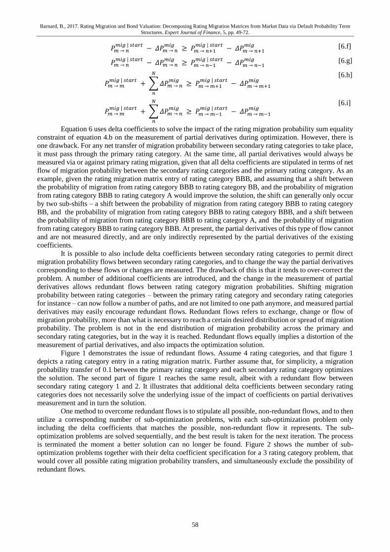
Figure 1 demonstrates the issue of redundant flows. Assume 4 rating categories, and that figure 1

depicts a rating category entry in a rating migration matrix. Further assume that, for simplicity, a migration

probability transfer of 0.1 between the primary rating category and each secondary rating category optimizes

the solution. The second part of figure 1 reaches the same result, albeit with a redundant flow between

secondary rating category 1 and 2. It illustrates that additional delta coefficients between secondary rating

categories does not necessarily solve the underlying issue of the impact of coefficients on partial derivatives

measurement and in turn the solution.

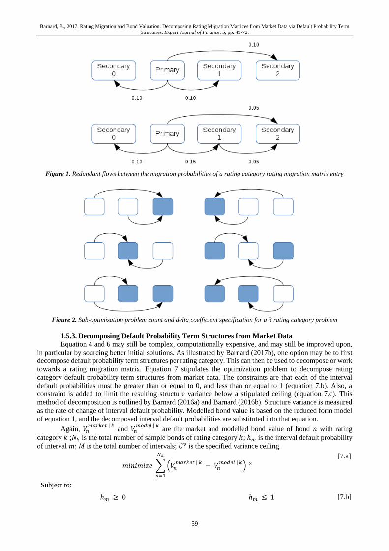
One method to overcome redundant flows is to stipulate all possible, non-redundant flows, and to then

utilize a corresponding number of sub-optimization problems, with each sub-optimization problem only

including the delta coefficients that matches the possible, non-redundant flow it represents. The sub-

optimization problems are solved sequentially, and the best result is taken for the next iteration. The process

is terminated the moment a better solution can no longer be found. Figure 2 shows the number of sub-

optimization problems together with their delta coefficient specification for a 3 rating category problem, that

would cover all possible rating migration probability transfers, and simultaneously exclude the possibility of

redundant flows.



59

Figure 1. Redundant flows between the migration probabilities of a rating category rating migration matrix entry

Figure 2. Sub-optimization problem count and delta coefficient specification for a 3 rating category problem

1.5.3. Decomposing Default Probability Term Structures from Market Data

Equation 4 and 6 may still be complex, computationally expensive, and may still be improved upon,

in particular by sourcing better initial solutions. As illustrated by Barnard (2017b), one option may be to first

decompose default probability term structures per rating category. This can then be used to decompose or work

towards a rating migration matrix. Equation 7 stipulates the optimization problem to decompose rating

category default probability term structures from market data. The constraints are that each of the interval

default probabilities must be greater than or equal to 0, and less than or equal to 1 (equation 7.b). Also, a

constraint is added to limit the resulting structure variance below a stipulated ceiling (equation 7.c). This

method of decomposition is outlined by Barnard (2016a) and Barnard (2016b). Structure variance is measured

as the rate of change of interval default probability. Modelled bond value is based on the reduced form model

of equation 1, and the decomposed interval default probabilities are substituted into that equation.

Again, 𝑉𝑛𝑚𝑎𝑟𝑘𝑒𝑡 | 𝑘

and 𝑉𝑛𝑚𝑜𝑑𝑒𝑙 | 𝑘

are the market and modelled bond value of bond 𝑛 with rating

category 𝑘 ;𝑁𝑘 is the total number of sample bonds of rating category 𝑘; ℎ𝑚 is the interval default probability

of interval 𝑚; 𝑀 is the total number of intervals; 𝐶𝑣 is the specified variance ceiling.

𝑚𝑖𝑛𝑖𝑚𝑖𝑧𝑒 ∑ (𝑉𝑛𝑚𝑎𝑟𝑘𝑒𝑡 | 𝑘


)

𝑁𝑘

𝑛=1

2

[7.a]

Subject to:

ℎ𝑚 ≥ 0 ℎ𝑚 ≤ 1 [7.b]



60

∑ (ℎ𝑚+1 − ℎ𝑚)2

𝑀−1

𝑚=1

≤ 𝐶𝑣

[7.c]

As part of the optimization, market bond value – as opposed to modelled bond value – can also be

based on a market based interest rate term structure instead – an interest rate term structure decomposed from

market data. Instead of its quoted price, the market value of a bond is taken to be the resultant value when

discounting the bond against the market based interest rate term structure. This assumes the decomposed

market interest rate term structure ideally represents the market outlook, and this renders bond issues' residual

modelling error equal to zero. The benefit of this is that it reduces idiosyncratic bond value error, thereby

simplifying the problem. This also shifts the focus from merely a portfolio of bonds to an interest rate term

structure instead, such that the objective may be expressed as decomposing the corresponding default

probability term structure of an interest rate term structure, and vice versa, rather than decomposing the default

probability term structure of a portfolio.

Furthermore, when market bond value is based on a decomposed interest rate term structure, and the

number of issues are sufficient, and adequately spaced in terms of maturity, it is also possible to calculate a

default probability term structure by means of a sequential (bootstrapping) method that iteratively seeks the

next interval default probability that minimizes modelled issue value error. The mechanics of the sequential

method is easy to follow when considering an issue with such a maturity that it is only affected by one interval

default probability – in this case, the default probability term structure (applicable to the issue) only spans one

interval, and can be calculated through iterative searching. When ordering issues according to maturity, each

subsequent issue will then also have only one outstanding interval default probability, if it adopts the default

probability term structure of the preceding issues and intervals.

1.5.4. Decomposing Rating Migration Matrices from Default Probability Term Structures

The following stipulates the method to decompose rating migration matrices from default probability

term structures, rather than from bond issue value. Decomposing from default probability term structures

instead, may imply smoother data, and that the default probabilities of the rating categories are already known

– according to equation 2, first interval default probability equals the default probability of the rating category

(Barnard, 2017a; Barnard, 2017b). This in turn implies it is only necessary to decompose the non-default

migration probabilities of the rating migration matrix.

Equation set 8 contains the general optimization problem. The optimization problem optimizes a

solution rating migration matrix, and interval default probabilities are modelled from the solution rating

migration matrix by means of equation 2. The constraints included are: a) for each rating category, the sum of

the probabilities of migrating from the particular category to any other non-default category, plus the

probability of default of the category should equal 1 (equation 8.b, corresponding to equation 4.b); b) for each

rating category, any probability of migrating to any other non-default category, as well as the probability of

default of that particular category should be greater than or equal to zero (equation 8.c and equation 8.e,

corresponding to equation 4.c); c) for each rating category, the probability of migrating to rating category 𝑛

should be equal to or greater than the probability of migrating to rating category 𝑛 + 1, if rating category 𝑛

succeeds the rating category; and for each rating category, the probability of migrating to rating category 𝑛

should be equal to or greater than the probability of migrating to rating category 𝑛 − 1, if rating category 𝑛

preceeds the rating category (equation 8.d, corresponding to equation 4.e); d) for each rating category with a

rating category preceding it, the particular category's probability of default should be equal to or higher than

that of the category preceding it (equation 8.f, corresponding to equation 4.d). Equation 8 would face the same

issues discussed under section 1.5.2, and should be implemented with delta coefficients, as outlined under

section 1.5.2 and equation 6.

𝑁𝑘 is the number of intervals of rating category 𝑘; ℎ𝑛𝑚𝑎𝑟𝑘𝑒𝑡 | 𝑘

and ℎ𝑛𝑚𝑜𝑑𝑒𝑙 | 𝑘

are the decomposed

market and modelled inteval default probabilities of interval 𝑛 and rating category 𝑘, respectively; 𝑃𝑚 → 𝑛𝑚𝑖𝑔

is

the probability of rating category 𝑚migrating to rating category 𝑛; 𝑃𝑐𝑎𝑡𝑚

𝑑𝑒𝑓𝑎𝑢𝑙𝑡 is the probability of rating category

𝑚 defaulting.

𝑚𝑖𝑛𝑖𝑚𝑖𝑧𝑒 ∑ (ℎ𝑛𝑚𝑎𝑟𝑘𝑒𝑡 | 𝑘

− ℎ𝑛𝑚𝑜𝑑𝑒𝑙 | 𝑘

)

𝑁𝑘

𝑛=1

2

[8.a]

Subject to:



61


𝑛=1 + 𝑃𝑐𝑎𝑡𝑚

𝑑𝑒𝑓𝑎𝑢𝑙𝑡 = 1; 𝑚 ∈ { 1, . . , 𝑐𝑎𝑡𝑛𝑜𝑛−𝑑𝑒𝑓𝑎𝑢𝑙𝑡 } [8.b]


𝑛=1 ≥ 0; 𝑚 ∈ { 1, . . , 𝑐𝑎𝑡𝑛𝑜𝑛−𝑑𝑒𝑓𝑎𝑢𝑙𝑡 } [8.c]

𝑃𝑛 → 𝑛−𝑥𝑚𝑖𝑔

≥ 𝑃𝑛 → 𝑛−𝑥−1𝑚𝑖𝑔

𝑃𝑛 → 𝑛+𝑥𝑚𝑖𝑔

≥ 𝑃𝑛 → 𝑛+𝑥+1𝑚𝑖𝑔

𝑛 ∈ (1, . . . 𝑐𝑎𝑡𝑛𝑜𝑛−𝑑𝑒𝑓𝑎𝑢𝑙𝑡)

𝑛 − 𝑥 ≤ 𝑐𝑎𝑡𝑛𝑜𝑛−𝑑𝑒𝑓𝑎𝑢𝑙𝑡; 𝑛 − 𝑥 − 1 ≥ 1

𝑛 + 𝑥 + 1 ≤ 𝑐𝑎𝑡𝑛𝑜𝑛−𝑑𝑒𝑓𝑎𝑢𝑙𝑡; 𝑛 + 𝑥 ≥ 1

[8.d]


𝑑𝑒𝑓𝑎𝑢𝑙𝑡 ≥ 0 [8.e]


𝑑𝑒𝑓𝑎𝑢𝑙𝑡≥ 𝑃𝑐𝑎𝑡𝑚−1

𝑑𝑒𝑓𝑎𝑢𝑙𝑡; 𝑚 ∈ { 2, . . , 𝑐𝑎𝑡𝑛𝑜𝑛−𝑑𝑒𝑓𝑎𝑢𝑙𝑡 } [8.f]

The overall optimization is conducted in two steps or procedures. The first step builds an initial

solution rating migration matrix, by sequentially optimizing the rating migration matrix entries of individual

rating categories, and by gradually increasing the percentage by which the rating migration matrix is applied

when determining the interval intensities and thus the interval default probabilities of a rating category. An

initial multiplier of 0 (0%) is used, and incremented to 1 (100%) through a step increment of 0.05 (5%). The

effect of this is that rating categories initially ignore the rating migration matrix entries of other rating

categories, and gradually adjust their rating migration matrix entries to that of the other rating categories. It

helps to ease the inter-dependency between rating categories – the dependency of a rating category on other

rating category rating migration matrix entries are controlled by the multiplier. The updated rating migration

entries of each rating category are stored in a temporary buffer for the next iteration. The first step implements

the optimization problem of equation 8, through delta-coefficients, and with additional delta-coefficients

realized by sub-optimization problems to prevent redundant flows, as outlined under section 1.5.2.

The outcome of the above step is a valid rating migration matrix that is partially optimized. To further

optimize this initial solution, two different optimization problems are used. Both optimization problems build

on equation 8. The first type simultaneously optimize the rating migration matrix entries of all rating

categories. It uses delta-coefficients, but only utilizes the primary delta-coefficient set, and does not include

delta-coefficients for secondary rating categories, and the corresponding additional sub-optimization problems.

The second type sequentially optimize the rating migration matrix entries of individual rating categories.

Additional delta-coefficients are used for secondary rating categories, through additional sub-optimization

problems. It essentially corresponds to the method used to build the initial solution rating migration matrix.

The only difference is that it does not use a multiplier – when optimizing the rating migration matrix entry of

a rating category, the rating migration matrix entries of other rating categories are not factored, but used as is.

The first optimization process attempts to simultaneously optimize rating migration matrix entries of

rating categories against each other. The second optimization process attempts to optimize the rating migration

matrix entry of an individual rating category against the existing rating migration matrix entries of other rating

categories. The outcomes are not the same. The solution is further optimized and improved by iterating

between the optimization processes. After optimizing the rating migration matrix entry of an individual rating

category against the rating migration matrix entries of the other rating categories, it becomes feasible again to

simultaneously optimize the rating migration matrix entries of all rating categories against each other, and vice

versa.

2. Methodology

The study examines the power and accuracy of the proposed method to decompose rating migration

matrices from market data, via decomposed default probability term structures. An existing, known rating

migration matrix is utilized, and it is investigated to what extent the original rating migration matrix can again

be surfaced by the method, when fed relevant data. The rating migration matrix naturally provides a reference

default probability term structure per rating category (equation 2). The rating category default probability term

structures, but not the original rating migration matrix, are provided to the method. In addition, the method is

provided with a portfolio of bonds, a risk-free term structure, and rating category recovery rates. From this the

value of the bonds can be calculated (equation 1), and the market value of the bonds are assumed equal to the

calculated value. In turn, the value of the bonds are used to decompose an interest rate term structure for each

rating category included in the bond portfolio, and a default probability term structure is decomposed for each

rating category from the corresponding rating category interest rate term structures. The decomposed rating

category default probability term structures should and do correspond with the reference rating category default

probability term structures. From the rating category default probability term structures, the default probability



62

of each rating category is obtained, such that it is only necessary to decompose the non-default rating migration

probabilities of the rating migration matrix.

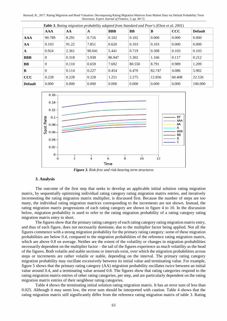
Seven principal credit ratings are considered – [AAA, AA, A, BBB, BB, B, CCC]. The study uses a

rating migration matrix from Elton et al (2001). The rating migration matrix is slightly adapted where it violates

some of the constraints mentioned as part of equation 4 and 8. Table 2 and table 3 show the original and

adapted rating migration matrix, respectively. In all cases that bond value is modelled, equation 1 is used to

calculate the value of the bonds. Recovery rates are taken from Elton et al (2001). Table 1 shows the recovery

rates used. The risk-free rate used is taken from Elton et al (2001) and Huang and Huang (2012). An artificial

portfolio of bonds is used, and the coupons of the bonds are set to 7.5. For each rating category, ten intervals

are considered, and the maturity of the issues are such that one issue matures per interval. Thus, 10 issues are

used per rating category, and 70 issues are used overall.

The actual decomposition of the rating category default probability term structures from the price data

of the bonds, via the rating category interest rate term structures, is not conducted here, but taken from Barnard

(2017b).

A simple barrier method is utilized to implement all optimization problems. However, an algorithm is

used to iteratively switch between optimization equations, and the best result per iteration is used as the initial

solution of the next iteration. Equation 9 notes the optimization equations used, in extension to the conventional

least-squares problem expression of equation 8.a, for example. Nevertheless, all optimization equation results

are still converted to, expressed, and compared in terms of the principal least-squares problem expression.

Equation 9.c and equation 8.a are identical. Equation 9.a applies a multiplier to the difference between

reference and modelled values. Equation 9.b considers absolute modelling error, instead of squared modelling

error, and equation 9.d and 9.e respectively penalize positive and negative modelling error more strongly.

𝑦 = ∑(𝑉𝑛𝑚𝑎𝑟𝑘𝑒𝑡 − 𝑉𝑛


𝑁

𝑛

⁄ 𝑎

𝑎 ∈ [1, 105, 1010]

[9.a]

𝑧 = | 𝑦 | [9.b]

𝑧 = (𝑦)2 [9.c]

𝑧 = (𝑦)𝑏1 + (𝑦)𝑏2

𝑏 ∈ [(4, 3), (8, 6)]

[9.d]

𝑧 = (𝑦)𝑏1 − (𝑦)𝑏2

𝑏 ∈ [(4, 3), (8, 6)]

[9.e]

Table 1. Recovery rates as percentage of par (Elton et al, 2001)

AAA AA A BBB BB B CCC

68.34 59.59 60.63 49.42 39.05 37.54 38.02

Table 2. Rating migration probability – Standard and Poor's (Elton et al, 2001)

AAA AA A BBB BB B CCC Default

AAA 90.788 8.291 0.716 0.102 0.102 0.000 0.000 0.000

AA 0.103 91.219 7.851 0.620 0.103 0.103 0.000 0.000

A 0.924 2.361 90.041 5.441 0.719 0.308 0.103 0.103

BBB 0.000 0.318 5.938 86.947 5.302 1.166 0.117 0.212

BB 0.000 0.110 0.659 7.692 80.549 8.791 0.989 1.209

B 0.000 0.114 0.227 0.454 6.470 82.747 4.086 5.902

CCC 0.228 0.000 0.228 1.251 2.275 12.856 60.637 22.526

Default 0.000 0.000 0.000 0.000 0.000 0.000 0.000 100.000



63

Table 3. Rating migration probability adapted from Standard and Poor's (Elton et al, 2001)


AAA 90.789 8.291 0.716 0.102 0.102 0.000 0.000 0.000

AA 0.103 91.22 7.851 0.620 0.103 0.103 0.000 0.000

A 0.924 2.361 90.041 5.441 0.719 0.308 0.103 0.103

BBB 0 0.318 5.938 86.947 5.302 1.166 0.117 0.212

BB 0 0.110 0.659 7.692 80.550 8.791 0.989 1.209

B 0 0.114 0.227 0.454 6.470 82.747 4.086 5.902

CCC 0.228 0.228 0.228 1.251 2.275 12.856 60.408 22.526

Default 0.000 0.000 0.000 0.000 0.000 0.000 0.000 100.000

Figure 3. Risk-free and risk-bearing term structures

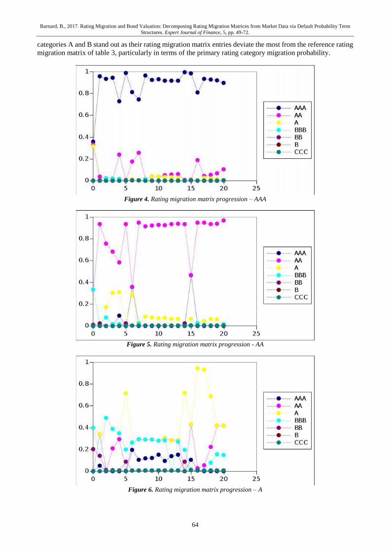
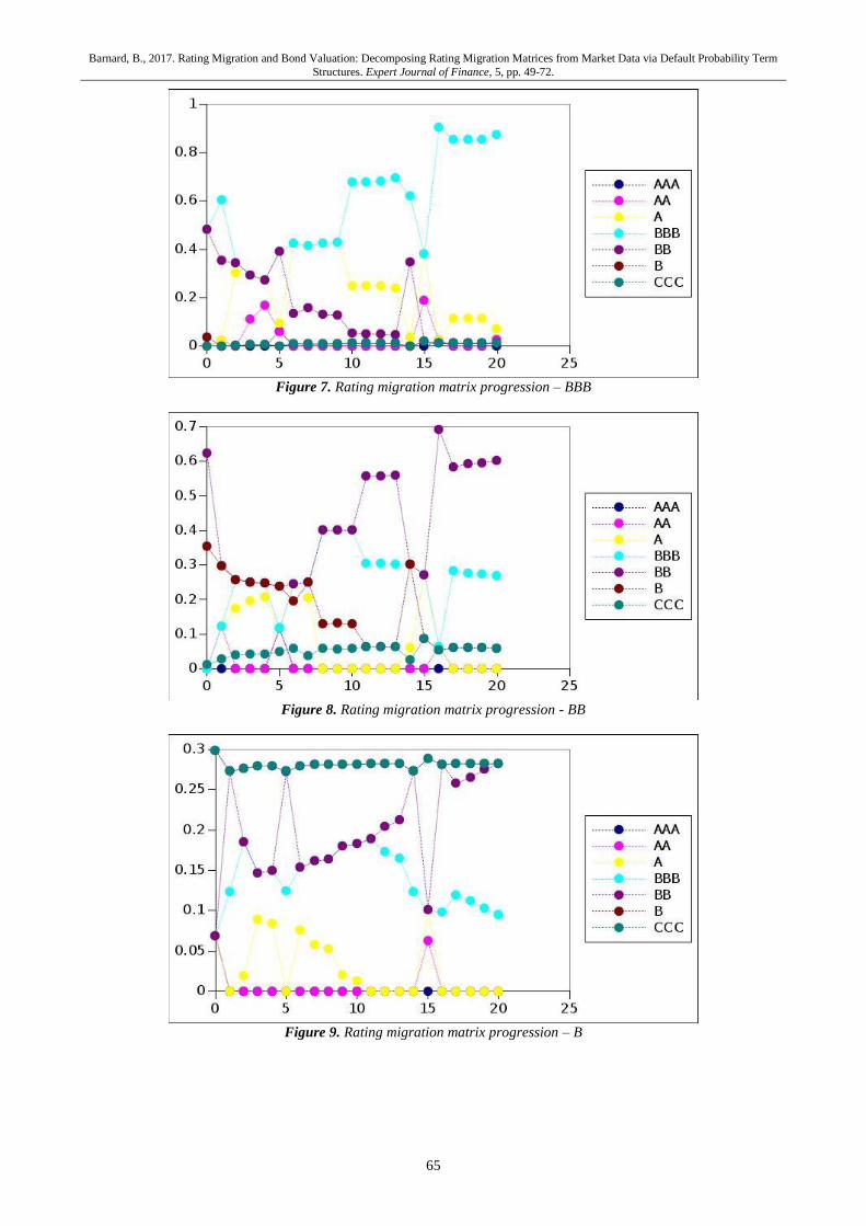
3. Analysis

The outcome of the first step that seeks to develop an applicable initial solution rating migration

matrix, by sequentially optimizing individual rating category rating migration matrix entries, and iteratively

incrementing the rating migration matrix multiplier, is discussed first. Because the number of steps are too

many, the individual rating migration matrices corresponding to the increments are not shown. Instead, the

rating migration matrix progressions of each rating category are shown in figure 4 to 10. In the discussion

below, migration probability is used to refer to the rating migration probability of a rating category rating

migration matrix entry in short.

The figures show that the primary rating category of each rating category rating migration matrix entry,

and thus of each figure, does not necessarily dominate, due to the multiplier factor being applied. Not all the

figures commence with a strong migration probability for the primary rating category: some of these migration

probabilities are below 0.4, compared to the migration probabilities of the reference rating migration matrix,

which are above 0.8 on average. Neither are the extent of the volatility or changes in migration probabilities

necessarily dependent on the multiplier factor – the tail of the figures experience as much volatility as the head

of the figures. Both volatile and stable sections or intervals exist, over which the migration probabilities across

steps or increments are rather volatile or stable, depending on the interval. The primary rating category

migration probability may oscillate excessively between its initial value and terminating value. For example,

figure 5 shows that the primary rating category (AA) migration probability oscillates twice between an initial

value around 0.4, and a terminating value around 0.8. The figures show that rating categories respond to the

rating migration matrix entries of other rating categories, per step, and are particularly dependent on the rating

migration matrix entries of their neighbour rating categories.

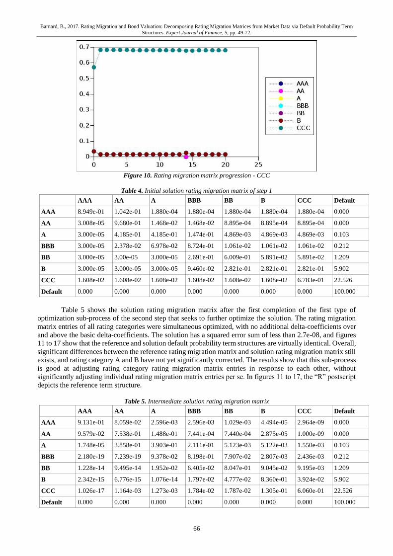
Table 4 shows the terminating initial solution rating migration matrix. It has an error sum of less than

0.025. Although it may seem low, the error sum should be interpreted with caution. Table 4 shows that the

rating migration matrix still significantly differ from the reference rating migration matrix of table 3. Rating



64

categories A and B stand out as their rating migration matrix entries deviate the most from the reference rating

migration matrix of table 3, particularly in terms of the primary rating category migration probability.

Figure 4. Rating migration matrix progression – AAA

Figure 5. Rating migration matrix progression - AA

Figure 6. Rating migration matrix progression – A



65

Figure 7. Rating migration matrix progression – BBB

Figure 8. Rating migration matrix progression - BB

Figure 9. Rating migration matrix progression – B



66

Figure 10. Rating migration matrix progression - CCC

Table 4. Initial solution rating migration matrix of step 1


AAA 8.949e-01 1.042e-01 1.880e-04 1.880e-04 1.880e-04 1.880e-04 1.880e-04 0.000

AA 3.008e-05 9.680e-01 1.468e-02 1.468e-02 8.895e-04 8.895e-04 8.895e-04 0.000

A 3.000e-05 4.185e-01 4.185e-01 1.474e-01 4.869e-03 4.869e-03 4.869e-03 0.103

BBB 3.000e-05 2.378e-02 6.978e-02 8.724e-01 1.061e-02 1.061e-02 1.061e-02 0.212

BB 3.000e-05 3.00e-05 3.000e-05 2.691e-01 6.009e-01 5.891e-02 5.891e-02 1.209

B 3.000e-05 3.000e-05 3.000e-05 9.460e-02 2.821e-01 2.821e-01 2.821e-01 5.902

CCC 1.608e-02 1.608e-02 1.608e-02 1.608e-02 1.608e-02 1.608e-02 6.783e-01 22.526

Default 0.000 0.000 0.000 0.000 0.000 0.000 0.000 100.000

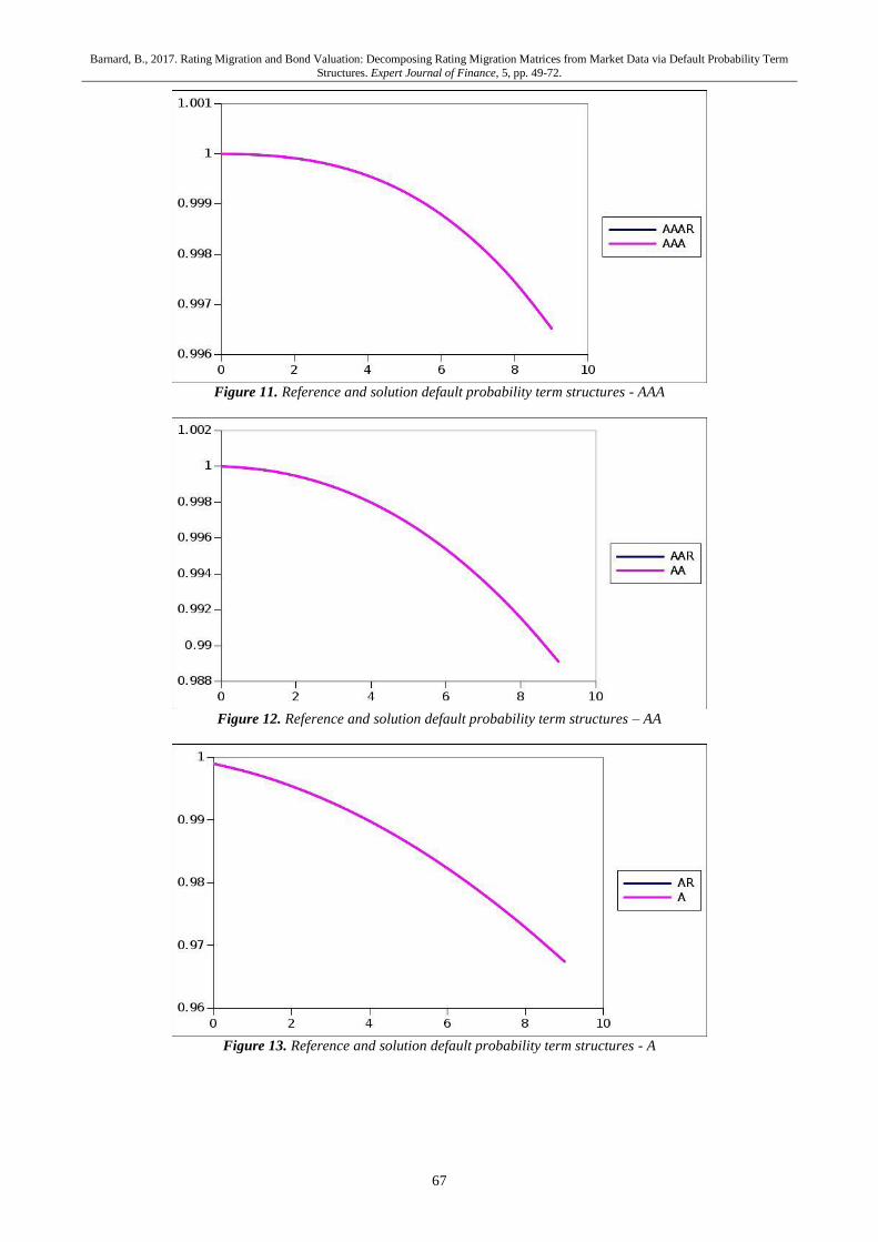
Table 5 shows the solution rating migration matrix after the first completion of the first type of

optimization sub-process of the second step that seeks to further optimize the solution. The rating migration

matrix entries of all rating categories were simultaneous optimized, with no additional delta-coefficients over

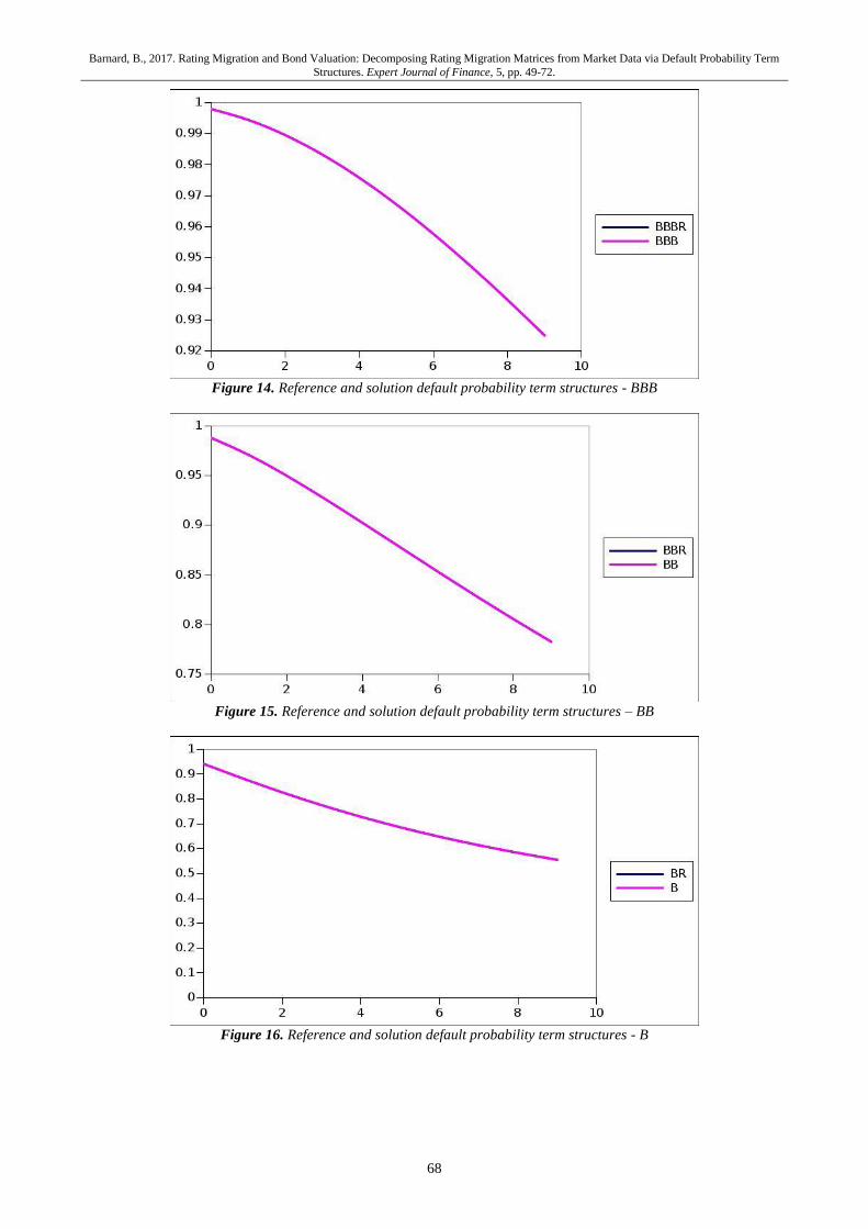
and above the basic delta-coefficients. The solution has a squared error sum of less than 2.7e-08, and figures

11 to 17 show that the reference and solution default probability term structures are virtually identical. Overall,

significant differences between the reference rating migration matrix and solution rating migration matrix still

exists, and rating category A and B have not yet significantly corrected. The results show that this sub-process

is good at adjusting rating category rating migration matrix entries in response to each other, without

significantly adjusting individual rating migration matrix entries per se. In figures 11 to 17, the “R” postscript

depicts the reference term structure.

Table 5. Intermediate solution rating migration matrix


AAA 9.131e-01 8.059e-02 2.596e-03 2.596e-03 1.029e-03 4.494e-05 2.964e-09 0.000

AA 9.579e-02 7.538e-01 1.488e-01 7.441e-04 7.440e-04 2.875e-05 1.000e-09 0.000

A 1.748e-05 3.858e-01 3.903e-01 2.111e-01 5.123e-03 5.122e-03 1.550e-03 0.103

BBB 2.180e-19 7.239e-19 9.378e-02 8.198e-01 7.907e-02 2.807e-03 2.436e-03 0.212

BB 1.228e-14 9.495e-14 1.952e-02 6.405e-02 8.047e-01 9.045e-02 9.195e-03 1.209

B 2.342e-15 6.776e-15 1.076e-14 1.797e-02 4.777e-02 8.360e-01 3.924e-02 5.902

CCC 1.026e-17 1.164e-03 1.273e-03 1.784e-02 1.787e-02 1.305e-01 6.060e-01 22.526

Default 0.000 0.000 0.000 0.000 0.000 0.000 0.000 100.000



67

Figure 11. Reference and solution default probability term structures - AAA

Figure 12. Reference and solution default probability term structures – AA

Figure 13. Reference and solution default probability term structures - A



68

Figure 14. Reference and solution default probability term structures - BBB

Figure 15. Reference and solution default probability term structures – BB

Figure 16. Reference and solution default probability term structures - B



69

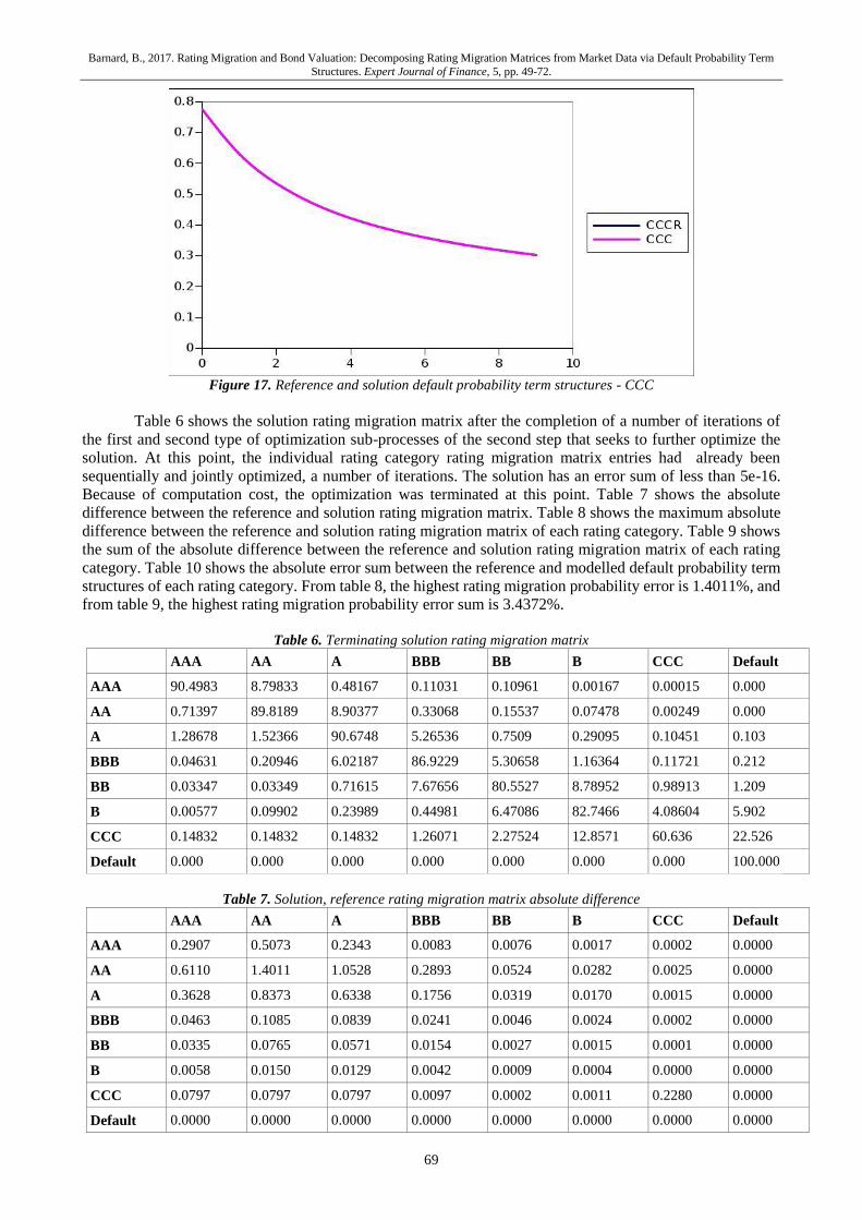
Figure 17. Reference and solution default probability term structures - CCC

Table 6 shows the solution rating migration matrix after the completion of a number of iterations of

the first and second type of optimization sub-processes of the second step that seeks to further optimize the

solution. At this point, the individual rating category rating migration matrix entries had already been

sequentially and jointly optimized, a number of iterations. The solution has an error sum of less than 5e-16.

Because of computation cost, the optimization was terminated at this point. Table 7 shows the absolute

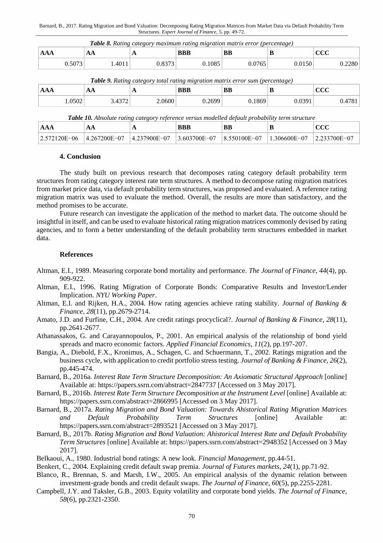
difference between the reference and solution rating migration matrix. Table 8 shows the maximum absolute

difference between the reference and solution rating migration matrix of each rating category. Table 9 shows

the sum of the absolute difference between the reference and solution rating migration matrix of each rating

category. Table 10 shows the absolute error sum between the reference and modelled default probability term

structures of each rating category. From table 8, the highest rating migration probability error is 1.4011%, and

from table 9, the highest rating migration probability error sum is 3.4372%.

Table 6. Terminating solution rating migration matrix


AAA 90.4983 8.79833 0.48167 0.11031 0.10961 0.00167 0.00015 0.000

AA 0.71397 89.8189 8.90377 0.33068 0.15537 0.07478 0.00249 0.000

A 1.28678 1.52366 90.6748 5.26536 0.7509 0.29095 0.10451 0.103

BBB 0.04631 0.20946 6.02187 86.9229 5.30658 1.16364 0.11721 0.212

BB 0.03347 0.03349 0.71615 7.67656 80.5527 8.78952 0.98913 1.209

B 0.00577 0.09902 0.23989 0.44981 6.47086 82.7466 4.08604 5.902

CCC 0.14832 0.14832 0.14832 1.26071 2.27524 12.8571 60.636 22.526

Default 0.000 0.000 0.000 0.000 0.000 0.000 0.000 100.000

Table 7. Solution, reference rating migration matrix absolute difference


AAA 0.2907 0.5073 0.2343 0.0083 0.0076 0.0017 0.0002 0.0000

AA 0.6110 1.4011 1.0528 0.2893 0.0524 0.0282 0.0025 0.0000

A 0.3628 0.8373 0.6338 0.1756 0.0319 0.0170 0.0015 0.0000

BBB 0.0463 0.1085 0.0839 0.0241 0.0046 0.0024 0.0002 0.0000

BB 0.0335 0.0765 0.0571 0.0154 0.0027 0.0015 0.0001 0.0000

B 0.0058 0.0150 0.0129 0.0042 0.0009 0.0004 0.0000 0.0000

CCC 0.0797 0.0797 0.0797 0.0097 0.0002 0.0011 0.2280 0.0000

Default 0.0000 0.0000 0.0000 0.0000 0.0000 0.0000 0.0000 0.0000



70

Table 8. Rating category maximum rating migration matrix error (percentage)


0.5073 1.4011 0.8373 0.1085 0.0765 0.0150 0.2280

Table 9. Rating category total rating migration matrix error sum (percentage)


1.0502 3.4372 2.0600 0.2699 0.1869 0.0391 0.4781

Table 10. Absolute rating category reference versus modelled default probability term structure


2.572120E−06 4.267200E−07 4.237900E−07 3.603700E−07 8.550100E−07 1.306600E−07 2.233700E−07

4. Conclusion

The study built on previous research that decomposes rating category default probability term

structures from rating category interest rate term structures. A method to decompose rating migration matrices

from market price data, via default probability term structures, was proposed and evaluated. A reference rating

migration matrix was used to evaluate the method. Overall, the results are more than satisfactory, and the

method promises to be accurate.

Future research can investigate the application of the method to market data. The outcome should be

insightful in itself, and can be used to evaluate historical rating migration matrices commonly devised by rating

agencies, and to form a better understanding of the default probability term structures embedded in market

data.

References

Altman, E.I., 1989. Measuring corporate bond mortality and performance. The Journal of Finance, 44(4), pp.

909-922.

Altman, E.I., 1996. Rating Migration of Corporate Bonds: Comparative Results and Investor/Lender

Implication. NYU Working Paper.

Altman, E.I. and Rijken, H.A., 2004. How rating agencies achieve rating stability. Journal of Banking &

Finance, 28(11), pp.2679-2714.

Amato, J.D. and Furfine, C.H., 2004. Are credit ratings procyclical?. Journal of Banking & Finance, 28(11),

pp.2641-2677.

Athanassakos, G. and Carayannopoulos, P., 2001. An empirical analysis of the relationship of bond yield

spreads and macro economic factors. Applied Financial Economics, 11(2), pp.197-207.

Bangia, A., Diebold, F.X., Kronimus, A., Schagen, C. and Schuermann, T., 2002. Ratings migration and the

business cycle, with application to credit portfolio stress testing. Journal of Banking & Finance, 26(2),

pp.445-474.

Barnard, B., 2016a. Interest Rate Term Structure Decomposition: An Axiomatic Structural Approach [online]

Available at: https://papers.ssrn.com/abstract=2847737 [Accessed on 3 May 2017].

Barnard, B., 2016b. Interest Rate Term Structure Decomposition at the Instrument Level [online] Available at:

https://papers.ssrn.com/abstract=2866995 [Accessed on 3 May 2017].

Barnard, B., 2017a. Rating Migration and Bond Valuation: Towards Ahistorical Rating Migration Matrices

and Default Probability Term Structures [online] Available at:

https://papers.ssrn.com/abstract=2893521 [Accessed on 3 May 2017].

Barnard, B., 2017b. Rating Migration and Bond Valuation: Ahistorical Interest Rate and Default Probability

Term Structures [online] Available at: https://papers.ssrn.com/abstract=2948352 [Accessed on 3 May

2017].

Belkaoui, A., 1980. Industrial bond ratings: A new look. Financial Management, pp.44-51.

Benkert, C., 2004. Explaining credit default swap premia. Journal of Futures markets, 24(1), pp.71-92.

Blanco, R., Brennan, S. and Marsh, I.W., 2005. An empirical analysis of the dynamic relation between

investment‐grade bonds and credit default swaps. The Journal of Finance, 60(5), pp.2255-2281.

Campbell, J.Y. and Taksler, G.B., 2003. Equity volatility and corporate bond yields. The Journal of Finance,

58(6), pp.2321-2350.



71

Cantor, R., Packer, F. and Cole, K., 1997. Split ratings and the pricing of credit risk. The Journal of Fixed

Income, 7(3), pp.72-82.

Chan, K. and Jegadeesh, N., 2004. Market-based evaluation for models to predict bond ratings. Review of

Pacific Basin Financial Markets and Policies, 7(02), pp.153-172.

Collin‐Dufresne, P., Goldstein, R.S. and Martin, J.S., 2001. The determinants of credit spread changes. The

Journal of Finance, 56(6), pp.2177-2207.

Das, S., and Tufano, P., 1995. Pricing Credit Sensitive Debt When Interest Rates, Credit Ratings, and Credit

Spreads Are Stochastic. Journal of Financial Engineering, 5, 161-198.

Delianedis, G. and Geske, R.L., 2003, February. Credit risk and risk neutral default probabilities: information

about rating migrations and defaults. In EFA 2003 annual conference paper (No. 962).

Duffee, G.R., 1999. Estimating the price of default risk. Review of Financial Studies, 12(1), pp.197-226.

Duffie, D. and Singleton, K.J., 1999. Modeling term structures of defaultable bonds. Review of Financial

studies, 12(4), pp.687-720.

Ederington, L.H. and Goh, J.C., 1998. Bond rating agencies and stock analysts: who knows what when?.

Journal of Financial and Quantitative Analysis, 33(04), pp.569-585.

Elton, J.E., 1999. Expected return, realized return and asset pricing tests. Journal of Finance, 4, pp.1199-1220.

Elton, E. J., Gruber, M. J., Agrawal, D. and Mann, C., 2001. Explaining the Rate Spread on Corporate Bonds.

The Journal of Finance, 56(1), pp.247-278.

Elton, E.J., Gruber, M.J., Agrawal, D. and Mann, C., 2004. Factors affecting the valuation of corporate bonds.

Journal of Banking & Finance, 28(11), pp.2747-2767.

Eom, Y.H., Helwege, J. and Huang, J.Z., 2004. Structural models of corporate bond pricing: An empirical

analysis. Review of Financial studies, 17(2), pp.499-544.

Ericsson, J., Jacobs, K. and Oviedo, R., 2009. The determinants of credit default swap premia. Journal of

Financial and Quantitative Analysis, 44(1), pp.109-132.

Fama, E.F. and French, K.R., 1993. Common risk factors in the returns on stocks and bonds. Journal of

financial economics, 33(1), pp.3-56.

Fei, F., Fuertes, A.M. and Kalotychou, E., 2012. Credit rating migration risk and business cycles. Journal of

Business Finance & Accounting, 39(1‐2), pp.229-263.

Foss, G.W., 1995. Quantifying risk in the corporate bond markets. Financial Analysts Journal, 51(2), pp.29-

34.

Frydman, H. and Schuermann, T., 2008. Credit rating dynamics and Markov mixture models. Journal of

Banking & Finance, 32(6), pp.1062-1075.

Grandes, M. and Peter, M., 2005. How Important is Sovereign Risk in Determining Corporate Credit Spreads

in Emerging Markets? The Case of Local Currency Bonds in South Africa. IMF Working Paper 217.

Geske, R.L. and Delianedis, G., 2001. The components of corporate credit spreads: Default, recovery, taxes,

jumps, liquidity, and market factors [online] Available at: http://escholarship.org/uc/item/32x284q3

[Accessed on 3 May 2017].

Hamilton, D.T. and Cantor, R., 2004. Rating transition and default rates conditioned on outlooks. Journal of

Fixed Income, 14(2), pp.54-70.

Hines, M.A., Ang, J.S. and Patel, K.A., 1975. Bond rating methods: Comparison and validation. The Journal

of Finance, 30(2), pp.631-640.

Houweling, P., Mentink, A. and Vorst, T., 2005. Comparing possible proxies of corporate bond liquidity.

Journal of Banking & Finance, 29(6), pp.1331-1358.

Houweling, P. and Vorst, T., 2005. Pricing default swaps: Empirical evidence. Journal of International Money

and Finance, 24(8), pp.1200-1225.

Huang, J.Z. and Huang, M., 2012. How much of the corporate-treasury yield spread is due to credit risk?.

Review of Asset Pricing Studies, 2(2), pp.153-202.

Jarrow, R.A. and Turnbull, S.M., 1995. Pricing derivatives on financial securities subject to credit risk. The

journal of finance, 50(1), pp.53-85.

Jarrow, R.A., Lando, D. and Turnbull, S.M., 1997. A Markov model for the term structure of credit risk

spreads. Review of Financial studies, 10(2), pp.481-523.

Jarrow, R.A., Janosi, T. and Yildirim, Y., 2002. Estimating expected losses and liquidity discounts implicit in

debt prices. Journal of Risk, 5(1), pp.1-38.

Kadam, A. and Lenk, P., 2008. Bayesian inference for issuer heterogeneity in credit ratings migration. Journal

of Banking & Finance, 32(10), pp.2267-2274.

Kaplan, R.S. and Urwitz, G., 1979. Statistical models of bond ratings: A methodological inquiry. Journal of

business, pp.231-261.



72

Kim, H., K. Ramaswamy, and S. Sunderesan, 1993. Valuation of Corporate Fixed-Income Securities.

Financial Management (Special issue on financial distress), 22(3), pp.60-78.

Kumar, K. and Haynes, J.D., 2003. Forecasting credit ratings using an ANN and statistical techniques.

International journal of business studies, 11(1), pp.91-108.

Lando, D. and Skødeberg, T.M., 2002. Analyzing rating transitions and rating drift with continuous

observations. Journal of banking & finance, 26(2), pp.423-444.

Longstaff, Francis A., and Eduardo S. Schwartz, 1995, A simple approach to valuing risky fixed and floating

rate debt. Journal of Finance, 50, pp.789-819.

Longstaff, F.A., Mithal, S. and Neis, E., 2005. Corporate yield spreads: Default risk or liquidity? New evidence

from the credit default swap market. The Journal of Finance, 60(5), pp.2213-2253.

Manzoni, K., 2004. Modeling Eurobond credit ratings and forecasting downgrade probability. International

Review of Financial Analysis, 13(3), pp.277-300.

Marciniak, M., 2006. Yield curve estimation at the National Bank of Poland; Bank i Kredyt; 10; p. 52-74

Merton, R., 1974. On the pricing of corporate debt: the risk structure of interest rates. Journal of Finance,

(May), 29(2), pp.449-470.

Nelson, C.R. and Siegel, A.F., 1987. Parsimonious modeling of yield curves. Journal of business, pp.473-489.

Nickell, P., Perraudin W. and Varotto, S., 2000. Stability of Rating Transitions. Journal of Banking & Finance,

24, pp.203-227.

Norden, L. and Weber, M., 2009. The co‐movement of credit default swap, bond and stock markets: An

empirical analysis. European financial management, 15(3), pp.529-562.

Wang, Z., 2004. Financial ratio selection for default-rating modeling: a model-free approach and its empirical

performance. Journal of Applied Finance, 14(1), pp.20-35.

Weistroffer, C., Speyer, B., Kaiser, S. and Mayer, T., 2009. Credit default swaps. Deutsche bank research.

Zhu, H., 2006. An empirical comparison of credit spreads between the bond market and the credit default swap

market. Journal of Financial Services Research, 29(3), pp.211-235.

http://creativecommons.org/licenses/by/4.0/

Rating Migration and Bond Valuation: Decomposing...

Documents

Transcript of Rating Migration and Bond Valuation: Decomposing...