RAPID 3-D RAYTRACING FOR OPTIMAL SEISMICSURVEY DESIGN

Jie Zhang

Earth Resources LaboratoryDepartment of Earth, Atmospheric, and Planetary Sciences

Massachusetts Institute of TechnologyCambridge, MA 02139

andBlackhawk Geometries, Inc.

Golden, CO 80401

Eugene Lavely

Blackhawk Geometries, Inc.Golden, CO 80401

M. Nafi Toksoz

Earth Resources LaboratoryDepartment of Earth, Atmospheric, and Planetary Sciences

Massachusetts Institute of TechnologyCambridge, MA 02139

ABSTRACT

A useful approach to optimal seismic survey design is to simulate the seismic responsefor a suite of a priori subsurface models and shot-receiver templates. The response canbe used to evaluate many criteria such as subsurface coverage, target resolution, noisesensitivity, aquisition footprint, data redundancy, long-wavelength statics resolution,and others. A key requirement for practical implementation is the use of an accurateand rapid simulation method. For most cases survey optimization for a highly detailed3D model would not be useful because (1) such information is often not available,(2) some of the conclusions may not be robust to small changes in the model, and(3) simulation of generally varying complex models would be prohibitively expensive.

3-1

Zhang et al.

Instead, a more useful model class for survey design would be 3D models with constantvelocity layers separated by arbitrary (and possibly complex) interfaces. The modelsmay be from conjecture or previous seismic surveys.

We present a rapid 3D raytracing method optimized for the computation of reflec­tion and refraction wavefronts from a point source in this model class. We demonstratethat the method simulates wave phenomena such as diffraction and head wave prop­agation. The approach is extremely fast since it avoids traveltime expansion in thevolume between interfaces, and solves a simple 2D problem on each interface. Othermethods require local propagators (even in constant velocity regions), whereas our ap­proach enables large jumps of wavefronts from interface to interface. The calculationof 3D reflection or refraction traveltimes for a model with an arbitrary interface fromone source to any number of receivers requires less than 1 sec of CPU time on a DEC3000/500 workstation.

We briefly review how our new method can be used to facilitate survey resolutioncomputations. We also develop a method for estimating an efficient source-receiverdistribution for resolving an assumed 3D structure. To design the receiver distribution,we calculate continuous traveltime slices at the surface from a given source templateand plot the RMS curvatures of the wavefronts. The spatial density of the receivercoverage should be in proportion to the locally-varying magnitude of the RMS curvature.Similarly, to determine the optimal source distribution, we sum the RMS curvatures ofthe wavefront traveltimes due to each source in the entire survey area. In the same way,the magnitude of the curvatures suggests the most important areas for source locations.

INTRODUCTION

The subsurface resolving capability of a 3-D seismic experiment and the acquisitioncost strongly depend on the survey design. In fact, on average, 75% of the costs of adomestic 3-D land survey are in the acquisition stages, 18% in processing and 7% ininterpretation. Clearly, an efficient survey design can yield significant acquisition sav­ings, and a data set optimized for the survey objectives will lead to reduced processingcosts, improved accuracy of interpretation, and ultimately, increased pay. Therefore,rigorous objective criteria for obtaining optimized 3-D data sets is critical for efficientand economic implementations. Of course, the goals of maximum resolution and mini­mum exploration cost are generally in conflict, so that survey design is a classic problemin optimization theory beset by trade-offs, uncertainties of assumptions, etc. Anothermajor problem is the identification of the appropriate objective criterion (or criteria)for assessing the utility of a given design. For example, the survey that can best resolvea given horizon may be suboptimal for AVO analysis, or the survey which yields well-resolved migrated images may display poor noise suppression capability. Thus, thechoice of the different criterion, their relative weighting, and the computational loadsare seen to be basic scientific problems. It is also necessary to weigh the trade-off be­tween objective criterion versus cost of acquisition. Finally, a major practical problem

3-2

(

(

(

(

(

(

(

Rapid 3-D Raytracing

efficient computation of such criteria. To gain industry acceptance, any survey designwork should represent only a small fraction of the total acquisition cost. This requires arapid and robust design implementation. A brute force method for survey design wouldbe to (1) perform a 3-D finite-difference calculation to generate a synthetic 3-D volumefor many source/receiver distributions, (2) run this data through the standard dataprocessing pipeline (including 3-D prestack depth migration), (3) evaluate the objectivecriteria, and repeat these steps for different designs and earth models. Nevertheless, weseek a more enlightened approach.

The determination of an efficient survey design for a given cost threshold requiresseveral important inputs including an a priori reservoir model for seismic response cal­culation, an objective criterion such as subsurface resolution, and a suite of shot-receivertemplates. For the purpose of survey design it is adequate to consider a simplified classof models e.g., constant velocity layers bounded by arbitrary interfaces. We develop a3-D raytracing method that can rapidly simulate reflection and refraction wavefrontsfor this model class. The goal is to provide a basic computational tool to facilitate thepractical implementation of any number of survey design methods on a PC. Our newray tracing method is presented in outline in the next section. The method is robust andself-contained so that it can be used in modular fashion in elaborate design optimizationprocesses that require ray tracing results (e.g. Beylkin et al., 1985; Barth and Wunsch,1990; Lavely et aI., 1997). These methods are for decimating shots and receivers in a3-D survey design without compromising the information content relative to that of areference survey with a dense distribution of shot-receiver pairs.

RAPID 3-D RAYTRACING METHOD

Simulation of typical 3D surveys would typically require ray path computations for0(105 )-0(106 ) source-receiver pairs. Furthermore, this computation will likely need tobe repeated for several input seismic models, and certainly for many source-receivertemplates. We have chosen the wavefront method to calculate traveltimes and raypathsin our 3-D models since the calculation time is independent of the number of receiversi.e., for a given source, raypaths and traveltimes are computed to all points in themodel including all points on the surface. Existing 3-D wavefront methods includefinite-difference approximations to the eikonal solution (e.g., Vidale, 1990; Hole andZeIt, 1995) and the shortest path methods by Saito (1990) and IGimes and Kvasnicka(1993). The later methods follows from the 2-D approaches of Saito (1989) and Moser(1989, 1991). These methods can be used to calculate traveltimes to all grid points incomplex velocity models. However, they do not provide computational savings when theinput models are simplified to the model class considered here (i.e. constant velocitylayers bounded by complex interfaces). This is because the solution of the eikonalequation with a finite-difference method is a local approach i.e., it must expand a localsquare wavefront progressively and cannot make large spatial jumps. The shortest pathmethod requires expansion along a virtual wavefront, and as with the finite-difference

3-3

(1)

Zhang et al.

method, cannot make large spatial jumps. The method that we present in what follows isuniquely suited for the restricted class of velocity models that we .consider. In essence, itcombines Snell's law with graph theory to expand directly wavefronts from one interfaceto another in a 3-D model.

The 3-D seismic model is gridded in horizontal directions (x and y) only. In thez dimension, the internal interfaces and the surface topography are defined as depthfunctions d( i, j) where the independent variables i and j are the grid coordinates for eachinterface. The functions d( i, j) may adopt any real value. This model representationresults in significant savings in the numerical implementation since 3-D volumes of dataneed not be stored. Instead we need only store a few 2-D vectors that define the interfacetopography, and 2-D traveltime and raypath vectors for each interface.

For the one interface problem, the method consists of the following steps:

1. Find any hidden areas on the interface that cannot be reached by straight raysfrom the source, and then compute 2-D traveltime vectors from the source to eachgrid point in the nonhidden areas using the straight rays.

2. If a refraction calculation is required. a directional graph template is applied tofind the shortest path connection on the interface, and then the refraction timesare accounted for.

3. Propagate the wavefront from the interface back to surface, using Snell's law toestimate up-going ray coverage for determining the size of a square graph template.

For the multiple interface problem, the propagator from interface to interface as estab­lished in step (3) can be used repeatedly to map traveltimes and raypaths from oneinterface to another either downward or upward.

The first step is not necessarily required for all models. However, hidden areas mayoccur when the interface has large depth variations. Detection of the hidden areas isimportant since raypaths in their vicinity may be complicated, and since diffractionsmay be generated from their edges. In practice, we seek the diffraction points firstand then determine the areas which are hidden behind the diffractors. When the anglebetween the vector of an incident ray and the normal vector of a reflector is less than900

, the local reflector must be hidden from the source, i.e.,

n·Vcos e= IPI < 0 ---> hidden reflector

where n is the normal vector of a reflector, and V is a vector of the incident ray. Figuresla defines the notation. The simple vector operation in equation (1) efficiently definesthe location of diffraction points. At the same time we store n for further calculations.However, the above rule can only help us to find some of the hidden reflectors. Afterthose of the reflectors satisfying the above rule are found, a directional graph templateis applied to search others in vicinity which do not satisfy the above rule but are hiddenbehind those just found. That is, we seek to determine if any segment of the straight

3-4

(

(

(

(

Rapid 3-D Raytracing

ray path connection between the source and the node is under the interface. Figure 1bshows the shape of a graph template. Following the direction from the source location tothe diffraction point, a graph template extends its coverage until no more hidden pointsare found. After all hidden points are found, their times t(i,j) are assigned a very largedefault value, and all remaining points are timed with straight rays from the source. Inperforming seismic traveltime calculations with graph theory, a graph template is used toselect nodes for updating traveltimes (Saito, 1989, 1991; Moser, 1989, 1990). However,here we apply a variable graph template to select nodes for finding hidden areas. Thisapproach allows us to deal with nodes, uniformly, automatically and efficiently. Wewill show later that other graph templates are also designed at different stages in thisrapid raytracing calculation. We apply the graph templates on the interfaces, and thetemplate is three-dimensional for non-planar interfaces. However, from the plan view,it is a 2-D problem, and indeed, we only need to solve a .2-D problem.

If a refraction computation is required, we continue to work on the interface andapply another graph template to find the critical refraction points and their connec­tions with other nodes. This turns out to be extremely simple with a graph template.Figure 2 illustrates a graph template with a fixed number of nodes but variable shapesat different locations. At each point on the interface, we use this graph template toupdate the times from a master point if necessary. Assuming that the time at themaster point (n, m) is t(n, m) and the minimum time between the master point andthe current working node (i,j) on the template is tT> we apply the following algorithm:

for any point (i,j) on the graph template:if [t(n, m) + t r < t(i,j)] then(1) t(i,j) = t(n, m) + tr

(2) ipath(i,j) = n + (m - l)nxendif

where ipath(i,j) is a vector for storing raypaths, t(i,j) may be a direct traveltimefrom the source or updated refraction time from other master point. Because we searchfor a minimum-time connection from all possible neighbors using a graph template, thealgorithm does not require that we order the nodes in any particular way. Therefore,we loop over all nodes on the interface without the need for sorting, and this representsa significant cost savings. This approach differs from the shortest path raytracing algo­rithms (Saito, 1989, 1990; Moser, 1989, 1991) since these require the application of thegraph template along the virtual wavefront. After applying the above algorithm we cantrack raypaths using the computed quantity ipath(i,j) and integrate refraction timeson the interface and the time from the source to point (i,j). The result updates t(i,j).

The third step is required for both reflection and refraction calculations. Wavefrontsfrom both ray types need to propagate back to the surface from the interface. In fact,mapping wavefront traveltimes from one interface to another and ultimately to thesurface is the primary concern of this study. First, nodes at the surface of the model

3-5

Zhang et al.

are assigned with a very large default value for reflection calculations, or with directtraveltimes for refraction calculations. We apply Snell's law to determine the directionsof rays propagating upwards from the interface. For this purpose, vector operations areefficient and reliable. We denote an up-going ray vector by if. To determine if, we mustconsider three different cases:

(1) reflection: if = P- 2(p· n)n(2) refraction: if= 1P1 cos,6 n+ sin,6 p(3) transmission: if = 1P1 (cos,6 - sin a cos a sin,6) n+ sin a sin,6 p

where a is the incident angle beneath the interface, and ,6 is the angle between if and n.We have assumed that 1<11 = 1P1. In the above formulation the amplitude is immaterial,and only the vector direction is required in the calculation. Formulas (2) and (3) aboveare for the case of refraction. Transmission from the lower to the upper medium occurswhen the angle of the refracted ray propagating upwards from the lower medium is lessthan 90°. The angles a and ,6 can be determined from the following relationships:

(

p·n (coso:

1P1(2)

sin ,6VI

(3)- sinaV2

where VI and V2 are the velocities in the upper and lower medium, respectively.Using the above algorithms, we first calculate if for every point on the interface. As

shown in Figure 3, the graph template size and location at the surface for each pointon the interface are determined by the ray directions of its four neighbor nodes. If thecomputed location of a graph template is not contained within the surface of the model,the default of the graph template is placed at the surface following if to calculate anypossible diffraction.

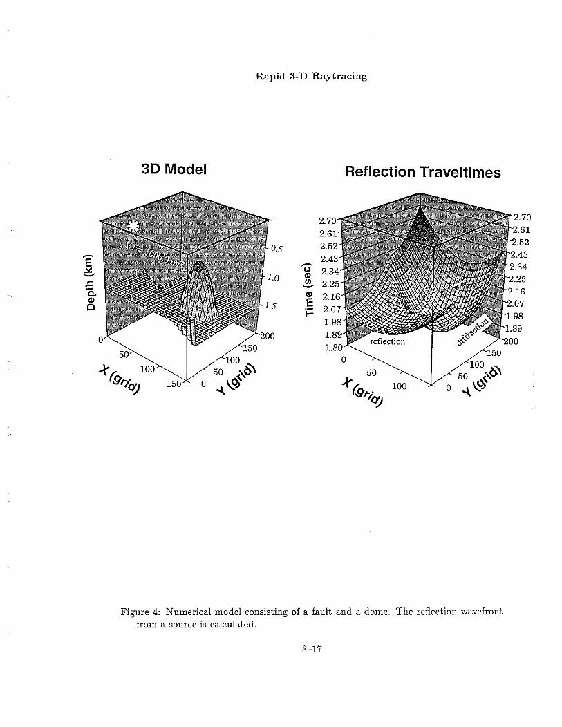
The above three-step approach is robust and efficient. It is sophisticated enough todeal with complex interface shapes. We design three different graph templates that canoptimize the calculation in three steps. The approach is computationally efficient sinceit is not necessary to perform a wavefront expansion within the 3-D volumes boundedby the internal interfaces. Figure 4 demonstrates a numerical example in which wecompute the traveltimes of a reflected wavefront for a dome model. The results clearlyillustrate that both wave phenomena (diffraction) and ray phenomena (reflection) aremodeled. Figure 5 shows a refraction calculation for a fault model. The diffraction effectfrom the edge of the fault is clearly evident in this example as well. The computationsin Figures 4 and 5 each required less than 1 sec of CPU time on a 160 MHz DEC-Alphaworkstation.

3-6

(

(

(

Rapid 3-D Raytracing

OPTIMAL SEISMIC SURVEY DESIGN

The computational efficiency demonstrated in the previous section is an important ad­vance since it makes optimized survey design computationally feasible. For a 3-D nu­merical model that is constructed from an a priori seismic model, we can calculatewavefront traveltimes for thousands of shots in less than 15 minutes of CPU time onour 160 MHz DEC-Alpha workstation. There are a number of ways to evaluate theutility of survey designs. First, we describe methods based on inverse theory, and thenpresent a method that may be used to estimate how a survey may be decimated withoutcompromising the data control on the subsurface structure. These methods strongly relyon ray tracing results, but are clearly impractical without the availability of a rapid,robust, and accurate ray tracer. Of course, for smaller scale problems, computationtime is less of a concern. For example, Barth and Wunsch (1990) computed the optimalexperimental deployment of sources and hydrophones for an ocean acoustic tomographicexperiment. They confined their attention to a total of nine sources and receivers andthe objective criterion they chose was to maximize the smallest singular value of thedesign matrix. They searched the experiment parameter space using a simulated an­nealing algorithm. They applied a global optimization technique, but their problem wasnonetheless tractable due to the limited parameter space, and the simplified physics ofocean acoustic wave propagation. In our problem, wave propagation will typically bemuch more complex, and the parameter space to be explored is vastly larger. Issues ofglobal optimization for 3-D surveys deserve study. However, in preface to this, it willbe helpful to simply restrict the parameter space, and evaluate the relative merits andtrade-ofts of a limited set of designs.

Use of Inverse Theory for Improved Survey Design

A qualitative approach to the analysis of acquisition geometry using, for example, vi­sualization of ray paths to ensure adequate bin coverage, can provide useful insights,but the results are difficult to quantify. On the other hand, we can draw on the resultsof inversion theory to obtain a more quantitative result. In fact, inverse theory canprovide a powerful framework for survey design optimization. Inverse methods maybroadly be classified into either (1) operator-based approaches such as migration, or(2) model-based approaches such as traveltime tomography. In conventional inversions,experimental design parameters are assumed fixed, and data are inverted for the desiredmodel. In design optimization, the experiment parameters are adjusted until a data setthat will yield a model solution with the desired properties is obtained. These may in­clude maximum model resolution, minimum model covariance, robustness to noise, andmany others. Operator-based inversion methods estimate model parameters directlyfrom the observed data using a specified mathematical model for wave propagation.Layer-stripping inversion, and migration are examples of operator-based inversion.

An example of operator-based inversion for improved survey design is given by Gib­son et al. (1994). They performed a modeling study to design a source configuration

3-7

Zhang et at.

which could be used to collect VSP data suitable for 3-D elastic wave Kirchoff migra­tion. Synthetic seismograms were computed for a variety of source configurations overa model of deep reflectors below the known shallow geology of the site. They thenapplied Kirchoff migration to these results, and were thereby able to assess the imagingpotential of possible future field experiments at the site.

An example of model-based inversion for improved survey design is given by Barthand Wunsch (1990) in the ocean acoustic experiment described above. Their goal was toresolve as well as possible the slowness values of voxels within a regular grid. In general,the appropriate objective criterion depend on the goals of the survey, but they showedthat many desirable solution properties may be achieved for surveys in which the designmatrix G has a condition number as near as possible to unity. Another way of statingthis is that the smallest singular value of G should be as large as possible. In their case,the inverse problem was given by G m = d where m are the desired slowness valuesand d is the data. They perturbed the source and receiver distribution using simulatedannealing until their objective function (the smallest singular value) was maximized.

We note that the studies of Gibson et al.(1994) and Barth and Wunsch (1990) bothrequired raytracing, and this was by far the most intensive computational element oftheir programs.

Inverse Theory and Survey Design Based on Generalized Radon Transform

Beylkin (1985) and Beylkin et al. (1985) presented a general approach to the descriptionof the spatial resolution of seismic experiments and migration (or inversion) algorithms.They considered the inverse scattering problem for the Helmholtz equation which gov­erns acoustic wave propagation. The theory allows for an arbitrary background mediumand arbitrary configuration of sources and receivers. They showed that the spatial reso­lution of a given point can be defined by the domain of coverage in the spatial wavenum­ber domain. This domain depends on a mapping into spatial wavenumber space of thefrequency band of the signal, and a functional that is dependent on the source-receiverconfiguration and on the background medium. Their detailed development reduces toa remarkably simple and intuitive result. Suppose the scatterer is described in objectspace by the function f(x) and that its Fourier transform is j(k) where k is the spatialwavenumber vector. Beylkin et al. find that an estimate fest(x) of f is given by

(

(

(

(

1/,- -k.xf.,t(x) = (27f)3 Dx f(k)e dk. (4)

The description of the domain of integration D x is, in fact, the estimate of spatialresolution. For a given point x in the medium, this description is given by the mapping

k = w[\7r(x,s) + \7r(x,r)]. (5)

This mapping is of fundamental importance for survey design since the domain of inte­gration D x in equation (4) is defined by this expression for k. Here, w is the frequency,

3-8

Rapid 3-D Raytracing

x is the imaging point, s is the source location, r is the receiver location, \7r(x, s) isthe slowness vector at the imaging point connecting the source with that point, and\7r(x, r) is the slowness vector connecting the imaging point with the receiver. Thesum of the slowness vector terms defines a vector that bisects the angle defined by theray segments. This defines the direction of the wavenumber vector that can be recoveredfor this particular source-receiver pair. The result in equation (5) defines the resolutionof seismic imaging for a given experiment.

It is important to realize that the above results comes from a solution to the seismicinverse problem using the Generalized Radon Transform. In most inverse problems itis only possible to estimate resolution by actually inverting a matrix (e.g., Barth andWunsch, 1990) which can be numerically intensive and unstable. Here, however, weare able to estimate resolution by performing forward ray tracing computations. Thisis a powerful advantage for the routine and practical use of this method, especiallywith the availability of a rapid 3-D ray tracer. Lavely et al. (1997) used the results inequations (4) and (5) to develop simple and intuitive methods of evaluating competingsurvey designs. They concentrated on the effect of limited aperture on coverage in thespatial wavenumber domain. The recovery without distortion of a point scatterer inobject space would, in general, require complete source-receiver coverage on a surfacesuch as a sphere that encloses the point. In addition, all frequencies are required, thebackground model must be perfectly known, and all unmodeled wave phenomena shouldbe accounted for or filtered from the data. If all of these conditions were met but onlylimited signal bandwidth is available, then instead of a point image, we would recovera finite size object with half-width determined by the finite frequency bandwidth. Inreality none of the above conditions are met and so we only recover a distorted andband-passed image of the object.

Method for Decimating Surveys

We present a method to estimate a deployment of sources and receivers that accountsfor the spatially varying rate of seismic data. The principal idea is that regions with highdata curvatures should have dense coverage so that important structural information canbe resolved, whereas regions with low data curvatures should have sparser coverage sothat acquisition costs can be reduced. Thus, the goal is to decimate surveys in regionswhere variations are linear or smooth so that loss of independent data informationis minimized, and to oversample selected regions so that required resolution can beachieved.

The approach we use is straightforward. First, we compute reflection and/or re­fraction wavefronts for a fixed subsurface model (as defined earlier). We then use thecomputed traveltimes for further analysis. The above computation is performed for afinite number of sources but with an extremely dense receiver distribution. The highdensity receiver distribution is used so that we may calculate "continuous" traveltimeslices on the surface. This yields a data set with maximum information content, whichcan be used as the reference data set so that the effects of decimation may be eval-

3-9

Zhang et al.

uated later. We then compute two functionals from the traveltime results, the RMSreceiver-time curvature and the source-time curvature. The first functional measuresthe complexity of wavefront traveltime variation to every point in the survey field fromall shots. The second functional measures the complexity of wavefront traveltime varia­tion to all receivers from each shot. We use these functionals to determine a decimatedsource and receiver distribution that meets the resolution requirement of the survey,but at reduced cost.

To measure the complexity of a traveltime slice, we calculate the spatial curvatureof the traveltimes using a Laplacian operator. We accumulate the traveltime curvaturesfrom n surface sources and define a functional of the RMS receiver-time curvatures forthe entire survey area:

(

(

(6)

where Ti is the traveltime slice due to ith source, and the derivatives are evaluated atthe receiver locations (x, V). The functional c,.(x, y) is a local quantity whose value ata given receiver is dependent on the source distribution but independent of the receiverdistribution. Thus, for a given source distribution, c,.(x, y) can be used to design anoptimal receiver layout. For example, a relatively large value of c,. at point (x, y)suggests there may be large traveltime variations in this vicinity, and therefore, a densereceiver distribution there would be advisable. We note that survey design conclusionsare simplified by the fact that only the relative magnitude of the functional is relevant.

We now consider SOurce distribution optimization for a survey with a fixed numberof receivers. To do this, we define a functional of the RMS source-time curvatures:

(

(7)(

where again j is the receiver index, m is the total number ofreceivers, (Xj, Yj) is the jthreceiver location, and the derivatives of Ti from source i are evaluated at the receiverlocations (Xj, Yj). The above functional simply sums the traveltime curvatures at all thereceiver points due to a single shot located at (Xi, Vi)' Therefore, Cs(Xi, Vi) depends onthe entire receiver distribution, but is independent of the other shot distribution. Thecalculation in equation (7) is repeated for all possible shot locations. For a fixed receivertemplate, a 2D contour of the resulting function Cs(Xi, Vi) can then be used to design anoptimal source distribution. If Cs(Xi, Vi) is relatively large, it suggests that there shouldbe a high density of shots in the vicinity of (Xi, Vi), or at least that selected shots therewill be important for generating significant features in the recordings. Thus, one canuse the relative magnitudes of Cs(Xi, Vi) to define a non-uniform source distribution thatwill increase resolution and decrease costs. Costs can be decreased by decimating theshot distribution in regions of relatively low Cs(Xi, Vi) values.

3-10

(

Rapid 3-D Raytracing

In Figure 6, we provide a numerical example using the above approaches to surveyoptimization. Figures 6a and 6b show a dome model with a constant overburden velocityof 1000 m/s. We calculate the functionals in equations (6) and (7) for two differentcases. In the first case, we assume that the sources and receivers for a reflection surveyare confined to a square surface area of 200 x 200 (m2 ). We uniformly populate thesurvey grid with sources in 4 m increments in both the x and y directions for a total of2500 sources. We then compute traveltimes for all of these sources to a set of receiverlocations that are coincident with the source locations. The total calculation takesabout 18 min on a DEC 3000/500 workstation. It is important to note that the CPUtime for the wavefront method is independent of the number of receivers. In the secondcase, we assume there is a square exclusion zone in which sources and receivers may notbe deployed. This reduces to 1900 the .total number of shots.

Figure 6c shows the contour of the RMS receiver-time curvatures with the highestmagnitude in the central circle for the first case. This calculation assumes that a sourcetemplate with 50 x 50 shot points has been selected, and that one wishes to understandhow receivers should be distributed for effective coverage. The figure shows that for thecase of uniformly distributed shots, the most important receiver locations are near thetop of the dome. Figure 6d illustrates the functional of the RMS source-time curvatures.This figure can be used to determine the most effective source locations. It suggeststhat these locations start from the central area and progressively expand outward. Thisconclusion is for the case in which receivers are uniformly distributed through the squaresurvey field.

In a real field survey there will be numerous culturally sensitive areas in whichsources or both sources and receivers must be excluded. The method we have developedis capable of handling arbitrarily shaped exclusion zones. Figures 6e and 6f shows anexample of an exclusion zone in the upper-right corner of the survey. Therefore, wecalculate the functionals in equations (6) and (7) in the remaining area. If sources areuniformly distributed in the available region we observe that the important locationsfor deploying receivers start from the top of the target and expand outward and alsoslightly downward as shown in Figure 6e. On the other hand, if receivers are uniformlydistributed in the open field, Figure 6f shows that the important source locations startfrom the central contour and expand over a slightly larger area along an axis betweenthe upper-left and the lower-right corners.

The approach we described is flexible since it can be used for any source-receivertemplate. One can rapidly explore many variations of the survey parameters and assessthe effectiveness of each combination. Because of its extremely high efficiency, theapproach can be also in a near real-time basis during field operations to improve surveydesign. For example, after receivers are deployed and a few shots are detonated, onecan replace some of the synthetic traveltimes with real data and repeat the calculationof the curvature functionals to improve the estimate. It is also important to note thatthe approach evaluates the continuity of wavefronts in 3D media and honors many waveeffects. The absolute traveltimes from an a priori model may not be reliable, and are

3-11

Zhang et al.

avoided in the functionals for survey design. The design approach is robust and requiresminimal input from the user, only an assumed source template for determining receiverlocations, an assumed receiver template for determining source locations, and an a priorisubsurface model. These requirements are not unreasonable.

CONCLUSIONS

We developed a rapid 3-D raytracing method for calculating wavefront traveltimes insimplified Earth models. Unlike conventional wavefront approaches, this method mapswavefronts directly from one interface to another i.e., it does not require incrementalupdating or spatial expansion within the constant velocity layers that define the seismicmodel. Therefore, the method is extremely fast, and brings the computationally inten­sive effort of optimal seismic survey design a step closer to practical implementation.The method can serve as a computational module for numerous design methods. Wedescribed some of these approaches, and introduced a new design method as well. Themethod involves estimating resolution capability by calculating RMS residuals betweenone shot record and others. The speed of this approach presents the opportunity tomake near real-time decisions in the field for routine use.

ACKNOWLEDGMENTS

The authors gratefully acknowledge the Gas Research Institute for support of this re­search for the Gas Research Institute for Advanced Seismic Data Acquisition and Pro­cessing under Contract # 5096-210-3781. We also thank Dr. Timothy Fasnacht, ourprogram manager at GRI, for advice and feedback. This work was also supported bythe Reservoir Delineation Consortium at the Massachusetts Institute of Technology.

3-12

(

(

(

(

Rapid 3-D Raytracing

REFERENCES

Barth, N. H. and Wunsch, C., 1990, Oceanographic experiment design by simulatedannealing, J. Phys. Ocean., 20, 1249-1263.

Beylkin, G., 1985, Imaging of discontinuities in the inverse scattering problem by inver­sion of a causal generalized Radon transform. J. Math. Phys., 26, 99-108.

Beylkin, G., Oristaglio, M. and Miller, D., 1985, Spatial resolution of migration al­gorithms, in Berkhout, A.J., RIdder, J., and van del' Wall, L.F., eds., AcousticalImaging, 14, Pleum Press, New York, pp. 155-167.

Gibson, Jr., R.L., Lee, J.M., Toks6z, M.N., Dini, 1. and Cameli, G.M., 1994, The appli­cation of 3D Kirchoff migration to VSP data from complex geological settings, 63rdAnn. Internat. Mtg. Soc, Explo. ,Geophys. Expanded Abstracts, 1290-1293.

Hole, J. A. and Zeit, B. C., 1995, 3-D finite-difference reflection traveltimes, Geophys.J. Int., 121, 427-434.

IGimes, L. and Kvasnicka, M., 1993, 3-D network ray tracing, Geophys. J. Int., 116,726-738.

Lavely, E. M., Gibson, Jr., R. L. and Tzimeas, C., 1997, 3D seismic survey design foroptimal resolution, submitted to SEG Expanded Abstracts for Fall, 1997 meeting.

Moser, T. J., 1989, Efficient seismic ray tracing using graph theory, Soc. ExplorationGeophys. 1989 Meeting, Expanded Abstracts, SEG, 'lUIsa, OK, 1106-1031.

Moser, T. J., 1991, Shortest path calculation of seismic rays, Geophysics, 56, 59-67.Saito, H., 1989, Traveltimes and raypaths of first arrival seismic waves: computation

method based upon Huygens' principle, Soc. Exploration Geophys. 1989 Meeting,Expanded Abstracts, SEG, 'lUIsa, OK, 244-247.

Saito, H., 1990, 3-D ray tracing method based on Huygens' principle, Soc. ExplorationGeophys. 1990 Meeting, Expanded Ebstracts, SEG, 'lUIsa, OK, 1024-1027.

Vidale, J., 1990, Finite-difference calculation of traveltimes in three dimensions, Geo­physics, 55, 521-526.

3-13

a)

\---.",~- \,, I

Zhang et al.

b)

(

(

(

(

Figure 1: (a) Notation of a normal vector for a reflector, incident ray and their angle.(b) Graph template to determine hidden nodes behind a diffraction point. Thesearch starts from the diffraction point and extends away from the source directionuntil no hidden points are found.

3-14

Rapid 3-D Raytracing

o master node

• working node

Figure 2: Refraction graph template on an interface. The number of working nodes isfixed for each master node, but the template shape varies according to its relativelolcation to source point.

3-15

Zhang et al.

Figure 3: Graph template on the surface for mapping up-going wavefront traveltimes.The size and shape of the template are determined by the up-going rays from themaster node on the interface and also from its four neighbor nodes.

3-16

(

(

(

(

(

(

(

Rapid 3-D Raytracing

3D Model Reflection Traveltimes

2.70 2.70

2.61 2.61

Os 2.52 2.52.-. 2.43 2.43E .-. 2.34:::. u 2.34(I)

s::. III 2.252.25--..... 2.16a. (I) 2.16(I) E0 2.072.07

i=1.98

1.98

1.891.89

200200

50150 1.80

150100 0 100..r(( 100 50 ~,o:-- 50 50 -,0:--9riC1j 150 0 ~,,~ ..r 100 0 ,,0}f{;,.,- ~1C1j

Figure 4: Numerical model consisting of a fault and a dome. The reflection wavefrontfrom a source is calculated.

3-17

(

Zhang et at.

3D Model Refraction Traveltimes

0.0 1.00.9

1.0 0.80.9 0.7-- 0.8 0.6e -- 0.7 0.5~ 0

-" O.) Q)0.6 0.4til$:. -"....

Q) 0.5 0.30. ,Q) e 0.4 0.2

,0 i= diffraction _0.3

200 0.2 200150 0.1 150

100. S"- 0.0 100. S"-O 50 '!-.." 0 50 '!-.." (

50 O~'S 50 O~'SX(grid)

100X (grid)

100150 150

(

(

Figure 5: Numerical model consisting of a fault. The refraction wavefront from a sourceis calculated.

(

3-18

(

Rapid 3-D Raytracing

a) plan view of a dome model

0,---------,

100

dapth=40m

200+-~~~,..~~~--lo 100 200 (m)

c) RMS receiver-time curvature

b) cross-section

0,-------,10

20

30

40+---/50+~~~,..~~~--1

o 100 200(m)

... d) RMS source-time curvature

1) RMS source-time curvaturein open survey area

e} RMS receiver-time curvaturein open survey area

closedatea ~

oclosedarea

Figure 6: Numerical simulation for optimal survey design. (a) Plan view of a domemodel. (b) Cross-section of the model. (c) Distribution of RMS receiver-time cur­vatures (see text for definition) when the sources are uniformly placed in the surveyarea, the central contour represents the highest magnitude. (d) Distribution of RMSsource-time curvatures (see text for definition) when the receivers are uniformlyplaced in the survey area, the central contour represents the highest magnitude. (e)Distribution of RMS receiver-time curvatures when a small area is not available forsurvey. (f) Distribution of RMS source-time curvatures when a small area is notavailable for survey.

3-19

Zhang et at.

3-20

(

(

(

(