RANSE Calculation of Laminar-to-Turbulent Transition-Flow around Sailing

Yacht Appendages

Christoph Böhm, R&D-Centre Univ. Applied Sciences Kiel, Yacht Research Unit, Germany

Kai Graf, Institute of Naval Architecture, University of Applied Sciences Kiel (UAS), Germany

ABSTRACT

A new method to simulate laminar-turbulent

transition has been used to study flow around sailing yacht

appendages. Based on an empirical correlation, the method

allows to predict transitional flow in a fully 3D-

environment using unstructured grids and massive

parallelization. Reynolds number of the flow around the

appendages of sailing yachts is of an order where

transitional flow plays an important role. The method thus

serves as a highly valuable tool for realistic optimisation of

yacht appendages.

The paper describes briefly Menters γ-ReΘ-

transition-model and shows its validity for the given

purpose. 2D-analysis of NACA-profiles has been chosen to

validate the transition model. The resulting lift and drag

coefficients from the RANSE calculations have been

compared with experimental data and results from the 2D-

boundary layer code XFoil, showing reasonable

agreement. The method then has been used for a bulb

length optimisation of an appendage configuration of an

ORC GP42 level racer. Here the differences between a

fully turbulent and a laminar turbulent optimisation are

shown and discussed.

NOTATION

(1+k) form factor

ARef reference surface

cD drag coefficient

cF,Hughes friction line according to Hughes

D drag force

DK destruction term of k equation

KD~

modified destruction term of k equation

Dω destruction term of ω equation

Eγ1 destruction term of transition sources

Eγ2 destruction term of relaminarization sources

gi component of mass normalized body force

k turbulent kinetic energy

K flow acceleration coefficient

L reference length

p pressure

PK production term of k equation

KP~

modified production term of k equation

Pγ1 production term of transition sources

Pγ2 production term of relaminarization sources

tP ,

~Θ source term to make t,eR

~Θ match ReΘ,t

Pω production term of ω equation

Re Reynolds number LU∞/ν Rec critical Reynolds number

ReΘ momentum thickness Reynolds number ΘU0/ν

ReΘ,c critical momentum thickness Reynolds number

ReΘ,t transition onset momentum thickness Reynolds

number ΘtU0/ν

t,eR~

Θ local transition onset momentum thickness

Reynolds number RT viscosity ratio

Rey Reynolds number based on wall distance

Reν vorticity Reynolds number

Sij strain rate tensor

S absolute value of strain rate, wetted surface

Tu turbulence intensity

U∞ freestream velocity

ui local velocity component

U0 velocity outside of boundary layer

y wall distance

y+ dimensionless wall distance

γ Intermittency

δ boundary layer thickness

δ* displacement thickness

δij Kronecker delta ε turbulence dissipation rate

θ boundary layer momentum thickness

λ0 pressure gradient coefficient

µ =ν ρ

µt =νT ρ

µτ friction velocity

ν kinematic viscosity

THE 18th

CHESAPEAKE SAILING YACHT SYMPOSIUM

ANNAPOLIS, MARYLAND, MARCH 2007

νT Turbulent viscosity

ρ Density

σi constants in diffusion coefficients

τ wall shear stress

τij Reynolds stress tensor

ω specific turbulence dissipation rate

Ω Absolute value of vorticity

Ωij vorticity tensor

INTRODUCTION

RANSE simulations of flow around sailing yacht

appendage systems are nowadays common practice in the

design stage of high performance sailing yachts. They are

used by many flow scientists and yacht designers to

optimize the shape of yacht keels, ballast bulbs, rudders

and wings. Modern RANSE codes offer great flexibility

taking into account viscosity, turbulence and free surfaces,

providing results that can compete with towing tank and

wind tunnel test results.

A common procedure in the analysis of flow

around appendages is to assume fully turbulent flow

allowing to use conventional turbulence models. However

the Reynolds number of typical yacht appendages is of an

order of magnitude where large laminar regions can be

expected. In fact designers usually try to extend the

laminar region of the appendage set by suitable form

modelling to decrease viscous resistance. Consequently

flow analysis not taking into account laminar to turbulent

transition may lead to erroneous design results.

Late developments of turbulence models address

this problem. The most promising of these enhanced

turbulence models, the γ-ReΘ-Turbulence model which is

implemented in the commercial RANSE solver CFX, uses

a correlation-based transition model to predict production

and dissipation of turbulent kinetic energy and wall shear

stress, MENTER (2004). The correlation used in the

transition model is based on experiments to correctly

describe the transition location. The principal idea behind

this method is to compare free stream turbulence intensity

with the local Reynolds number based on boundary layer

momentum thickness. Integral quantities needed for this

transition criteria are approximated by local variables to

avoid numerical problems within a RANSE code.

This transition model is used in a research project

at YRU-Kiel to investigate the laminar-to-turbulent

transition flow around the appendages of an ORC 42 level

racer. The achieved results are compared with results for

fully turbulent flow. The ORC 42 has been used as a

benchmark since it features a small fin-keel and a medium

length ballast bulb, where laminar flow can be expected on

about 50% of it’s wetted surface. Goal of this investigation

is to show whether the conventional assumption of fully

turbulent flow is appropriate or if it may lead to wrong

determination of optimal geometric properties of the

ballast bulb.

The following chapters give an introduction to the

theory of both transitional flow and γ-ReΘ-Turbulence

model and finally two examples which demonstrate the

capability of the method to predict laminar-to-turbulent

transition.

TRANSITIONAL FLOW

Also the complex mechanism of transition from

laminar to turbulent flow, as well as turbulence itself is still

not fully researched, it is known, that the transition from

laminar to turbulent flow is caused by viscous instabilities,

which are developing in the shear layer. These instabilities

always increase downstream and depend only on the

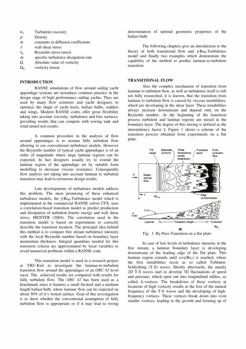
Reynolds number. At the beginning of the transition

process turbulent and laminar regions are mixed in the

boundary layer. The degree of this mixing is defined as the

intermittency factor γ. Figure 1 shows a scheme of the

transition process obtained from experiments on a flat

plate.

Fig. 1: By-Pass-Transition on a flat plate

In case of low levels of turbulence intensity in the

free stream, a laminar boundary layer is developing

downstream of the leading edge of the flat plate. This

laminar region extends until x=x(Rec) is reached, where

the first instabilities occur as so called Tollmien-

Schlichting (T-S) waves. Shortly afterwards, the mainly

2D T-S waves start to develop 3D fluctuations of speed

and pressure, which open out into longitudinal eddies, so

called Λ-vortices. The breakdown of these vortices at

locations of high vorticity results in the loss of the natural

frequency of the T-S waves and the developing of high-

frequency vortices. These vortices break down into even

smaller vortices, leading to the growth and forming up of

wedge-shaped turbulent spots. Turbulent spots move

downstream with the surrounding laminar boundary layer

and lead to an alternation between laminar and turbulent

flow, the intermittency as mentioned above. The

unification of the turbulent spots finally leads to a fully

turbulent boundary layer after exceeding the transition

Reynolds number Ret.

Transition to turbulence is mainly influenced by:

• Local Reynolds number

• Free stream turbulence intensity

• Pressure gradient

• Surface roughness

• Separation

For common yacht appendages the transition

length is usually much shorter than the overall length of

the appendage element. Consequently accurate prediction

of transition length is of less importance than prediction of

transition onset. Engineering methods for the prediction of

transition thus usually do not take into account the details

of the transition process. They rather predict the critical

Reynolds number Rnc and the transition Reynolds number

Rnt using empirical methods.

Most of these empirical methods are based on the

assumption that transition onset is linked to the Reynolds

number based on the momentum thickness of the boundary

layer. Empirical equations for the transition onset

momentum thickness Reynolds number are given by many

researchers. They take into account parameters describing

details of the flow as pressure gradient and freestream

turbulence intensity.

The general problem of implementing one of

these methods within RANSE codes is that RANSE

simulations use local information only for solving

governing equations. Derivation of integral values, which

are needed for determining the momentum thickness, is

troublesome and should be avoided.

Menters method to circumvent these problems is

based on a couple of ideas that allow him to calculate

transition from local variables only. His approach covers

many of the different aspects of transition:A new empirical

formulation for the transition onset momentum thickness

Reynolds number in the freestream is given.

• A transport equation is used to diffuse the

freestream transition onset momentum thickness

Reynolds number into the boundary layer.

• The momentum thickness Reynolds number is

correlated with the vorticity Reynolds number

which can be calculated from local variables

• An intermittency function is calculated from a

transport equation, the source term of this

equation depending on the transition onset

momentum thickness Reynolds number

• The intermittency function is used to manipulate

production and dissipation of turbulent kinetic

energy.

The following chapter outlines the basic equations

of this model and its integration into common RANSE

methods.

FLOW SIMULATION METHOD

The theory given here is a very brief outline of

Menters method. For details see the paper of

MENTER (2004).

Governing Equations

RANSE solver use a volume based method to

solve the time-averaged Navier-Stokes equations in a

computational domain around the investigated body. The

RANS equation evolves from time averaging mass and

momentum conservation for a continuous flow. In the

following method it is assumed that the Reynolds stress

evolving from time averaging is modelled using the eddy

viscosity hypothesis. Assuming incompressible flow this

yields, see FERZINGER (1991):

( )

i

i

j

j

iT

j

ij

iji

gx

u

x

u

x

x

kp

x

uu

t

u

+

∂

∂+

∂

∂+

∂

∂+

∂

+∂−=

∂

∂+

∂

∂

))((

)3/2(1

νν

ρ

ρ ( 1 )

0=∂

∂

i

i

x

u ( 2 )

Turbulence Model

The turbulence model used in the presented

approach calculates the turbulent viscosity νT from the

turbulent kinetic energy k and the specific turbulent

dissipation ω:

( )21

1

,max Fa

kaT

Ω=

ων ( 3 )

The turbulent kinetic energy k and the specific

turbulent dissipation rate ω are calculated using the γ-ReΘ-

Turbulence model shown below.

( ) ( ) ( )

∂

∂+

∂

∂+−=

∂

∂+

∂

∂

i

tk

i

kk

i

i

x

k

xDP

x

ku

t

kµσµ

ρρ ~~ ( 4 )

( ) ( )

( )

∂

∂+

∂

∂+

+−=∂

∂+

∂

∂

i

tk

i

t

k

i

i

xx

CdDP

x

u

t

ωµσµ

να

ωρρωωω

( 5 )

The γ-ReΘ-Turbulence model is equivalent to the

standard SST-Model besides having modified production

and destruction terms ( kk DP~

,~

) in the turbulent kinetic

energy equation. kP~

and kD~

are calculated from

production and destruction of turbulence in fully turbulent

regimes, Pk and Dk, and an intermittency function γ which

controls production and destruction of turbulent kinetic

energy depending on the transition onset momentum

thickness Reynolds number:

kEffk PP γ=~

( 6 )

kEffk DD )0.1),1.0,min(max(~

γ= ( 7 )

Transition-Model

The transition model assumes that the transition

onset momentum thickness Reynolds number outside the

boundary layer can be calculated by an empirical formula.

Menter suggests a new empirical correlation for ReΘ,t

which relates it to the freestream turbulence intensity Tu

and two empirical correlation factors λ0 and K. The

correlation is defined as:

[ ] ( )KFTut ,6067.073.803Re 0

027.1

, λ−

Θ += ( 8 )

ds

dU

Θ=

νλ

2

0 ( 9 )

ds

dU

UK

=

2

ν ( 10 )

The function for λ0 shows strong similarities to a pressure

gradient method proposed by Thwaites, whereas the

second parameter K is the so called acceleration parameter

similar to the method proposed by Mayle, for details see

WHITE (1991). The acceleration parameter K is used to

characterize the accelerations at the beginning of the

transition process. Function F(l0,K) is used to decide if a

polynomial function depending on λ0 or K is used to

determine ReΘ,t.

A local value of the transition onset momentum

thickness Reynolds number is calculated from a transport

equation, assuming that the freestream value of t,Reθ ,

calculated from ( 8 ), diffuses into the boundary layer:

( ) ( )( )

∂

∂+

∂

∂+=

∂

∂+

∂

∂ Θ

ΘΘ

ΘΘ

i

t

tt

i

t

i

tit

xxP

x

u

t

,

,,

,, eR~

eR~

eR~

µµσρρ

( 11 )

Here the source term tP ,Θ ensures that t,eR~

Θ

matches the local value of ReΘ,t outside the boundary layer,

the latter one obtained from ( 8 ). The source term Pθ,t

contains a blending function, which turns off the source

term in the boundary layer.

The transition onset momentum thickness

Reynolds number in the boundary layer, t,eR~

Θ , is related to

the critical momentum thickness Reynolds number c,Reθ ,

which is the Reynolds number where first instabilities in

the laminar boundary layer occur. Unfortunately this

relationship is proprietary and a hidden procedure within

Menters method:

( )tc f ,, eR~

Re Θ=θ ( 12 )

The critical momentum thickness Reynolds

number c,Reθ is now forwarded to the intermittency

transport equation, which controls the production and

destruction of turbulence in the turbulence model:

( ) ( )

∂

∂

+

∂

∂+−+−=

∂

∂+

∂

∂

if

t

ii

i

xxEPEP

x

u

t

γ

σ

µµ

γρργγγγγ 2211

( 13 )

In this transport equation, Pγ1 and Eγ1 depict the

transition sources necessary to start the production of

turbulence whereas Pγ2 and Eγ2 are the destruction or

relaminarization sources.

Pγ1 is controlled by an onset function which

depends on the ratio of the local momentum thickness

Reynolds number ΘRe and the critical momentum

thickness Reynolds number c,Reθ . To avoid the

calculation of the non-local momentum thickness Reynolds

number Menter uses a correlation between momentum

thickness Reynolds number θRe and the local vorticity

Reynolds number Reν:

193.2

ReRe

max,ν=Θ

( 14 )

Reν is based on local values only and can

therefore easily determined at each computational node:

Ω=µ

ρν

2

Rey

( 15 )

APPLICATIONS

In the following the method of Menter is validated

by comparing it with respective experimental and

numerical results from other sources. It is then used to

investigate the flow around the appendage set of an ORC

GP 42 level racer. While the first investigation assumes

planar flow, the appendage flow simulation is fully 3D.

The original empirical methods to predict transition from

the momentum thickness Reynolds number are 2D by

nature. However due to the substitution of integral values

with local variables fully 3D flow can be investigated with

Menters method. In addition, since the local transition

onset momentum thickness Reynolds number in the

boundary layer, t,eR~

Θ , is calculated from diffusion of the

freestream transition onset momentum thickness Reynolds

number, in-homogeneity of turbulence intensity in the

freestream can be taken into account. This allows to take

account of interaction of appendage elements like bulb and

blade or even blade and rudder.

2D TEST CASE: NACA 642-015 PROFILE

A profile of the well researched NACA 6-series

was chosen for analysis to verify the capability of the γ-

ReΘ-Turbulence model to predict transition. The results of

the profile analysis have been compared with experimental

data collected from Abbott/Doenhoff, ABBOTT (1959)

and numerical results generated by the well known profile

code XFOIL of DRELA (2001).

The simulation has been performed using a

hexahedral mesh with C-grid topology and approx. 180000

computational nodes. As an important pre-conditions to

achieve accurate results using the γ-ReΘ-Turbulence model

the dimensionless wall distance has to be restricted to Y+ ≤

1. Thus the wall nearest node of the grid has to be placed at

a distance of approximately 0.003 mm from the surface to

achieve correct results for a Reynolds number of 3*106.

Consequently great care has to be taken in the design of

the profile surface, which has to be very smooth to allow

proper gridding of the cells in the vicinity of it.

Fig. 2 shows the hexahedral mesh, the inset

showing grid resolution at the profile leading edge.

A sweep of angle of attacks from 0° to 10° have

been tested at constant inflow speed. Turbulence intensity

in the freestream has been set to 0.85%, which corresponds

to an Ncrit-Value of 3.012 in the XFoil settings. The exact

Turbulence level at which the experiments were conducted

in the wind tunnel is unknown, however Abbott/Doenhoff

mentioned it to be in the order of a few hundredths of one

percent.

Fig. 2: Grid around NACA 642-015 profile

Fig 3 shows the drag coefficient cD over angle of

attack AoA for RANSE calculation (both laminar-turbulent

and fully turbulent), XFOIL calculations and experimental

data. Drag coefficient cD is calculated by dividing the drag

force obtained from the computation with dynamic

pressure and the planform area.

f

DAU

Dc

Re

25.0 ⋅⋅⋅=

∞ρ ( 16 )

0.0E+00

2.0E-03

4.0E-03

6.0E-03

8.0E-03

1.0E-02

1.2E-02

1.4E-02

1.6E-02

1.8E-02

2.0E-02

0 2 4 6 8 10AoA [°]

CD [-]

CD XFOIL CD CFX

CD EXP CD CFX Turb

Fig. 3: Drag coefficient cD for NACA 642-015

Generally the RANSE results show rather good

compliance with both numerical and experimental

comparative data, in particular close to the non-lifting

condition AoA=0°. This is a good indicator for proper

laminar to turbulent transition prediction. Here the results

from the new transition model almost coincides with the

experimental data at angles from 0 to 2 degrees. Compared

to the experimental results the beam of the drag bucket is

narrower for the RANSE results, however comparing the

RANSE results with those from XFOIL, the trend is

inversed. Additional experimental results are needed here

to evaluate the merit of RANSE compared to XFOIL

results.

For wider angles of attack, the curves for the laminar-

turbulent RANSE calculations show a different slope than

the comparative data and quickly approach the results from

the fully turbulent RANSE calculation. In this region the

need for further research in order to determine possible

flaws in the calculation setup and to calibrate the model is

obvious. It is also worth considering that the quality of the

experimental and numerical comparative data itself is

unknown.

Fig. 4 compares transition points on top and bottom of the

surface resulting from numerical calculations with CFX

and XFoil. It can be nicely seen that the curve slopes are

very similar. Given the fact that XFOIL predicts narrower

drag bucket than the RANSE calculations, the horizontal

shift of the top transition points are very plausible.

0

0.1

0.2

0.3

0.4

0.5

0.6

0.7

0.8

0.9

1

0 2 4 6 8 10AoA [°]

Xtr/c [-]

Xtr/c Pressure Side XFOILXtr/c Suction Side XFOILXtr/c Pressure Side CFXXtr/c Suction Side CFX

Fig. 4: Transition Points on upper and lower profile

surface as predicted by CFX and XFOIL

In general the agreement between the different

methods compared here seems to be reasonable. This holds

particularly for a situation, where design input from an

optimisation has to be generated. Comparing variants of

topologically similar geometries like ballast bulbs of

different volume distribution or length will give quite

reasonable trends as long as the simulation set-up is not

changed.

Fig. 5 shows porcupine-plots representing the

wall shear stress on the profile. The upper plot depicts a

profile in fully turbulent flow, visible by a smoothly

decreasing distribution of wall shear stress in flow

direction. In the lower plot the result for a laminar-

turbulent transition simulation is shown.

Fig. 5: Wall Shear Stress on NACA 642-015 profile:

a) fully turbulent flow b) laminar-turbulent flow

Here the wall shear stress progression shows the

typical characteristic of laminar to turbulent transition: a

sharp increase close to the stagnation point followed by a

distinct shear stress decrease over almost 60% of the chord

length. The transition to turbulent flow can be identified at

the location where shear stress starts to increase again

indicating turbulent flow in the backward region.

BULB LENGTH VARIATION

As a practical application a length variation of a

keel bulb configuration for an ORC GP 42 level class racer

will be presented here. When trying to predict the optimum

length for a ballast bulb of given buoyancy the following

problem occurs:

Bulbs optimised using fully turbulent CFD codes

are known to become very long and slender, whilst bulbs

which are optimised using methods capable to take into

account laminar turbulent transition (like wind tunnel

testing) tend to be too bulky. The reason for this is, that for

fully turbulent flow a prolongation of the bulb increases

frictional resistance only slightly as can be derived from

Fig. 5. For a bulb with a laminar region at the forward part

any prolongation increases only the region where turbulent

flow prevails, resulting in an over-proportional increase of

resistance. Of course the bulb resistance in fully turbulent

flow is generally higher than in laminar turbulent transition

flow.

For comparison the bulb length investigation is

carried out for laminar turbulent transition flow as well as

for fully turbulent flow. This allows to estimate the error

margin, giving a measure of the merits bound to the use of

the presented method.

Geometry

No complete design of a GP 42 racer has been

available at the YRU Kiel. Consequently the blade and the

benchmark bulb have been developed according to the

ORC GP42 level class rules with dimensions likely to be

used in reality. From estimation of blade dimensions and

weight a benchmark bulb with the following characteristic

properties has been derived:

CSYS 18 Benchmark

Length L [m] : 2.400

Wetted Surface S [m²] : 2.215

Vertical Center of Gravity VCB [m] : 0.154

Long. Center of Gravity LCB [m] : -0.323

Volume Vol [m³] : 0.170

Height H [m] : 0.326

Width B [m] : 0.482

B/H Ratio SQR [m] : 1.480

Maxium Draft MD [m] : 2.300 Tab. 1: Geometric properties of the benchmark bulb

The bulb variants are derived from the benchmark

geometry by affine distortion of the bulb length, height and

width. During the study the bulb volume and its squish

ratio (B/H-ratio) as well as the maximum draft remains

constant. The following variants have been developed:

L [m] S [m²] VCB [m] H [m] B [m] Vol [m³]

CSYS 18_V1 1.900 1.988 0.173 0.367 0.543 0.170

CSYS 18_V2 2.150 2.104 0.164 0.345 0.510 0.170

CSYS 18_V3 2.650 2.323 0.147 0.310 0.459 0.170

CSYS 18_V4 2.900 2.427 0.140 0.297 0.439 0.170

CSYS 18_V5 3.150 2.527 0.135 0.285 0.422 0.170 Tab. 2: Geometric properties of the bulb variants

Fig. 6 shows bulb variants in profile and sectional

view. One can see that the variants derived from the rather

moderate benchmark become more and more radical with

increasing respective decreasing length.

Fig. 6: Overview of the bulb variants

The bulbs come completely without chines and

have an asymmetric profile to keep the centre of gravity

low. This results in a rather flat bottom part.

Simulation Setup

The simulation has been set up in a boxed

environment similar to those encountered in wind tunnels,

with the following differences: The box walls are treated as

frictionless free slip walls and the appendage configuration

is tested in full scale, thus eliminating any problems with

Reynolds similarity. The boundary conditions applied are a

constant inflow speed of 5.144 m/s on the inlet, which is

corresponding to a speed of 10 knots. On the outlet von

Neumann condition (derivation of flow forces

perpendicular to the boundary is zero) is applied. The bulb

is investigated in downwind condition only, the free stream

turbulence intensity has been set to 0.85% as during the

profile investigation.

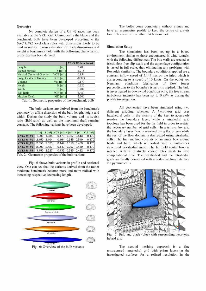
All geometries have been simulated using two

different gridding schemes: A hexa-tetra grid uses

hexahedral cells in the vicinity of the keel to accurately

resolve the boundary layer, while a tetrahedral grid

topology has been used for the far field in order to restrict

the necessary number of grid cells. In a tetra-prism grid

the boundary layer flow is resolved using flat prisms while

the rest of the flow domain is discretized using tetrahedral

cells. The first method consists of an inner box around

blade and bulb, which is meshed with a multi-block

structured hexahedral mesh. The far field (outer box) is

meshed with a relatively coarse tetra mesh to save

computational time. The hexahedral and the tetrahedral

grida are finally connected with a node-matching interface

via pyramid cells.

Fig. 7: Bulb and blade (blue) with surrounding hexa-tetra

hybrid grid

The second meshing approach is a fine

unstructured tetrahedral grid with prism layers at the

investigated surfaces for a refined resolution in the

boundary layer. This method has the advantage that it can

be easily adapted to any geometry, but comes with the

disadvantages that the task of resolving the correct

boundary layer height is not as easily performed as with

the hexahedral mesh and the computational effort is bigger.

Elements

Hexa-Tetra-

Hybrid Grid

Tetra-Prism

Grid

Hexa-Tetra-

Hybrid Grid

Tetra-Prism

Grid

Hexahedral 2784428 - 1512944 -

Tetra 828109 992155 1421511 992155

Prism - 4350902 - 869978

Pyramids 50656 158 41152 66

ΣΣΣΣ Elements 3663193 5343215 2975607 1862199

ΣΣΣΣ Nodes 2909960 2358636 1745740 618495

laminar-turbulent fully turbulent

Tab. 3: Grid parameters

Both grid variants have been developed with

approximately the same grid resolution, see Tab. 3. The

tetra-hexa grid has a computational load which is around

half a million nodes greater than with the tetra-prism grid.

This mainly owed to the fact that the tetra-prism grids

allows for more aimed node distribution and can therefore

save some nodes, whilst hexahedral grids always come

with some constraints that cause the grid size to increase.

The grids for the fully turbulent simulations are

generally around 40% (hybrid) – 70% (tetra-prism) smaller

than the laminar-turbulent grids. This is due to high

resolution needed in the boundary layer for the γ-ReΘ-

Transition model to work correctly. The differences

between the prism elements in fully turbulent and laminar

unstructured grids depict this very well, see Tab. 3.

Naturally this also enlarges the differences in node

numbers between the two grid approaches developed for

fully turbulent flow.

Fig. 8: Unstructured tetra grid with prism layer on bulb

and blade surfaces

It has to be mentioned that the meshing effort for

laminar-turbulent calculations is huge, since the grid

generator has to capture the intersections between bulb and

blade with the same high resolution as with the profile

investigation. Therefore it is even more important than for

the 2 D test case to invest great care in developing smooth

and clean surfaces.

Results Hexa-Tetra Grid

The computational results achieved with the hexa-

tetra grid suffer from a most unexpected drawback: a

review of the form factors shows that the pressure drag of

the bulb is heavily underestimated. The form factor is

defined as follows:

( )HughesF

D

c

ck

,

1 =+ ( 17 )

where cD is defined as in formula 14, but normalized using

the wetted surface instead of the planform area. The

coefficient cF,Hughes resembles the friction line as introduced

by Hughes.

( )( )2,2Relog

063.0

−=HughesFc ( 18 )

A length variation is usually an interplay between

the viscous drag, mainly depending on the wetted surface,

and the pressure drag, depending on the form of the

investigated body. A massive pressure underestimation

leads to a very blunt bulb, this being the body with the

least wetted surface. Obviously these results are useless as

they do not resemble reality.

0.85

0.90

0.95

1.00

1.05

1.10

1.15

1.20

1.8 2 2.2 2.4 2.6 2.8 3L [m]

F/F

Ben

ch, V

cg

/Vc

gB[-

]

Drag / DragBench

VCGBulb/VCGBench

Viscous Drag / VDragBench

Pressure Drag / PDragBench

Fig. 9: Results of fully turbulent length variation with

hexa-tetra-hybrid grid

Fig. 9 and Fig. 10 show the results for the fully

turbulent and the laminar- turbulent test run with the

hexahedral grid. All results have been modified in a way

that they depict the difference to the benchmark geometry

in percent. Besides total drag the curves for the resistance

components viscous and pressure drag, as well as the

development of the bulb vertical centre of gravity are also

given to show the different trends.

0.85

0.90

0.95

1.00

1.05

1.10

1.15

1.8 2 2.2 2.4 2.6 2.8 3L [m]

F/F

Ben

ch, V

cg

/Vc

gB [

-]

Drag / DragBenchVCGBulb/VCGBenchViscous Drag / VDragBenchPressure Drag / PDragBench

Fig. 10: Results of laminar turbulent length variation with

hexa-tetra-hybrid grid

In case of the fully turbulent length variation an

optimum was found, at a length of 2.15m, this being 0.25m

smaller than the benchmark bulb. This resulted in a bulb

which was bulkier than one would expect for a fully

turbulent calculation. The calculations taking laminar-

turbulent transition into account did not lead to an

optimum at all. Here the result was that any shortening of

length leads to decrease of resistance.

A thorough investigation of the simulation lead to

the conclusion that the problems have to be grid related.

Whether the problems arose from the mixing of tetra and

hexa grid, from the blocking structure or from the node

distribution could not yet be resolved. Currently we

assume the pressure underestimation to be related to

distortion of the hexa grid caused by the use of a

unconventional blocking strategy.

Results Unstructured Tetra-Prism Grid

The results received from the simulations with the

second meshing approach, using the tetra-prism grid, are

by far more encouraging. The problems of massive

pressure underestimation which occurred with the first grid

did not appear here and the ratio of pressure and viscous

drag looks very realistic.

Fig. 11 shows results for fully turbulent

calculations using the tetra-prism grid. Here an optimum of

total drag was acquired for a bulb length of 3.15m, which

is +0.75m longer than the benchmark bulb. The optimum

for the fully turbulent calculation is rather flat, however it

fits well with theory and common knowledge that this kind

of simulation does tend to produce long and needle-like

bulbs.

0.85

0.90

0.95

1.00

1.05

1.10

1.15

1.20

1.8 2.0 2.2 2.4 2.6 2.8 3.0 3.2L [m]

F/F

Ben

ch, V

cg

/Vv

gB[-

] Drag / DragBench

VCGBulb/VCGBench

Viscous Drag / VDragBench

Pressure Drag / PDragBench

Fig. 11: Length Variation with respect to Benchmark

Geometry CSYS18_BM (Fully Turbulent Mode)

The results of the simulations conducted with the

new laminar-turbulent-transition model are shown in Fig.

12. As to be expected, the pressure drag increases with

decreasing bulb length due to the bulkier shape of the

body. Simultaneously the viscous drag decreases because

the wetted surface of the body gets smaller. The optimum

distribution of pressure and viscous drag is reached for a

bulb length of 2.15m. This corresponds to a delta of -

0.25m to the benchmark. The optimum bulb length for a

bulb in laminar turbulent flow is about 1 m shorter than for

a bulb in fully turbulent flow.

0.85

0.90

0.95

1.00

1.05

1.10

1.15

1.20

1.25

1.8 2 2.2 2.4 2.6 2.8 3L [m]

F/F

Ben

ch,V

cg

/Vc

gB [

-]

Drag / DragBench

VCGBulb/VCGBench

Viscous Drag / VDragBench

Pressure Drag / PDragBench

Fig. 12: Influence of Length Variation with respect to

Benchmark Geometry CSYS18_BM (Laminar-Turbulent-

Transition Model)

Fig. 13 shows longitudinal location of transition

onset for the bulbs. The transition locations are measured

at bottom, top and side of the bulb and normalized with the

bulb length. An increase of bulb length decreases the

longitudinal position of the transition location quite

smoothly towards the bulb nose. The sole exception here is

bulb variant V3 which shows a unexpected peak on the

bulb bottom.

0.0

0.2

0.4

0.6

0.8

1.0

1.8 2.1 2.4 2.7 3.0L [m]

Xtr

/c [-]

Xtr/c Top

Xtr/c Bottom

Xtr/c Side

Fig. 13: Transition Points on bulb calculated with the γ-

ReΘ-Transition model

By comparing the results for the bulb top, bottom

and side, one can see that the changes are most distinctive

for the bulb top. This seems to be plausible since the top of

the bulb geometry is intersecting with the blade. Corner

vertices as well as transition on the blade may cause the

flow on the bulb top to transit earlier to turbulence thus

overriding the natural transition process.

Fig. 14 and Fig. 15 depict wall shear stress for the

benchmark bulb for fully turbulent flow and for laminar-

turbulent transitional flow. Fig. 14 shows shear stress

increasing from zero at the nose to maximum somewhere

behind mid section. Afterwards the wall shear stress

decreases towards the end.

Fig. 14: Contour plot of wall shear stress on benchmark

bulb (fully turbulent)

Fig. 15 shows a similar contour plot for laminar-

turbulent transition flow around benchmark bulb. Shear

stress is characterized by a sudden increase of wall shear

stress on the nose, followed by a swift decrease to a very

low level.

Fig. 15: Contour plot of wall shear stress on benchmark

bulb (laminar- turbulent)

This low level of shear stress is maintained until

the critical Reynolds number Rec is reached. From here the

wall shear stress increases to almost the same value as with

the fully turbulent calculation. It then follows the same

pattern as described for the fully turbulent calculation and

decreases towards the beaver-tail end of the bulb.

Fig. 16, Fig. 17 and Fig. 18 show turbulent kinetic

energy on the surface of the benchmark bulb, the V2

variant (very short bulb) and the V4 variant (very long

bulb) respectively. The images unveil the development of

laminar and turbulent zones for the three selected bulb

lengths. Here blue colour regions indicate laminar flow,

whilst regions of turbulent flow are coloured red. The

bulbs shown here are the benchmark bulb, the optimum-

length bulb for laminar turbulent transition flow (V2) and

the optimum-length bulb for fully turbulent flow (V4).

Fig. 16: Contour plot of turbulent kinetic energy on the

benchmark bulb indicating laminar (blue) turbulent (red)

flow

Flow at the bulb-blade junction of the benchmark

bulb transits relatively early to turbulent. By looking at the

transition course at blade and bulb, it seems that

instabilities of the flow on the bulb force the flow on the

blade to transit to turbulence forward of the natural

transition location.

The optimum bulb for laminar-turbulent transition

flow (Fig.17) possesses several differences compared to

the benchmark bulb. Noticeable is the rather late transition

of laminar to turbulent flow on the entire bulb surface. The

laminar-turbulent transition at the upper part of the bulb

surface is probably triggered by the flow instabilities on

the blade. However, late transition at the bulb side may be

a consequence of higher curvature and thus negative

pressure gradients compared to the benchmark.

Fig. 17: Turbulent kinetic energy on the V2 bulb

Fig. 18 shows the optimum-length bulb for fully

turbulent flow. One can see that the flow instabilities on

the upper part of the bulb surface are not strong enough to

force a transition on the blade surface. Instead the laminar

flow on the blade seems stable enough help in stabilizing

the laminar regions at the bulb regions near to the blade

junction. The comparatively weak instabilities on the bulb

top are probably owed to the position of maximum

thickness, which moves further aft for the longer bulbs.

Fig. 18: Turbulent kinetic energy on the V4 bulb

Fig.19 shows turbulent kinetic energy at bulb

bottoms for the entire range of investigated bulb lengths.

By comparison the different lengths of laminar and

turbulent regions can be detected easily.

It can be generally stated that the flow on the top

and bottom side of the bulb transits earlier to turbulent

flow than at the bulb sides. Furthermore, the contour of the

transit regions varies from a more or less even sectional

distribution around the shortest bulb (V1) towards a wedge

shape turbulent peak at bottom of the longest bulb (V4.)

This phenomena is surely owed to the geometry

of the bulb which was designed rather flat with a B/H ratio

of 1.48 in order to keep the centre of gravity low.

Additionally the bulb bottoms are flatter than the bulb tops.

This also enhances hydrostatic stability, but is not suited to

stabilize the laminar flow.

Fig. 19: Contour plot of kinetic energy on bulb bottom

The most obvious evidence for this theory is the

smallest bulb (Variant V1), of which the bottom and top

side show highest curvature. This introduces a laminar

region of almost equal length around the entire body.

A cut through the blade profile shown in the Fig.

20 demonstrates that the γ-ReΘ-Transition model is capable

of catching flow phenomena otherwise only seen in costly

experimental investigation. One can see that due to an

increase of pressure, which results in a loss of kinetic

energy (due to friction), the laminar boundary layer is no

longer able to maintain attached flow at the wall and

consequently separates. This triggers the boundary layer to

transit to turbulence, thus gaining additional momentum

which diffuses back into the now turbulent boundary layer

allowing it to reattach to the wall.

Fig. 20: Boundary layer profile at transition location

Conclusion

In this paper a new laminar-turbulent transition

model has been tested for its ability to predict laminar-to-

turbulent transition flow around yacht appendages. The

method consists of an empirical approach for the transition

onset momentum thickness Reynolds number and

correlations of integral values and local variables to be

solvable within a RANSE code.

The method has first been verified by comparing

results of a 2D-profile investigation with respective

investigations using a boundary layer method (XFOIL) as

well as experimental data. The drag coefficients from the

different data sources have been compared and the

agreement between them was found to be generally

sufficient.

The second test case, a length variation of a

typical ORC42 ballast bulb, successfully extends the

calculation to a fully 3D environment. The length

variation shows that the assumption of fully turbulent flow

does not only lead to a significant overestimation of the

flow forces, but – of even more importance –also may lead

to wrong determination of optimal geometric properties of

the ballast bulb.

It could be shown that the optimum low-drag

bulb length is significantly longer assuming fully turbulent

flow than the optimum bulb length determined taking

laminar regions on the bulb surface into account.

It has to be pointed out that this paper investigates

optimum bulb lengths with respect to resistance

minimization only. To maximize boat speed the impact of

bulb length on hydrostatic stability has to be taken into

account.

REFERENCES

Abott, I.H., v. Doenhoff, A.E. (1959): Theory of Wing

Sections, Dover Publications Inc., New York, 1959

Drela, M. (2001): XFOIL 6.9 User Primer,

http://web.mit.edu/drela/Public/web/xfoil/,

MIT Cambridge, 2001

Ferziger, J.H., Peric, M. (2002): Computational Methods

for Fluid Dynamics, Springer, New York 2002

Mayle, R.E. (1991): The Role of Laminar-Turbulent

Transition in Gas Turbine Engines, ASME Journal of

Turbo machinery, Vol. 113, 1991

Menter, F.R., Langtry, R.B., Likki, S.R., Suzen, Y.B.,

Huang, P.G., Völker, S. (2004): A Correlation Based

Transition Model Using Local Variables Part I – Model

Formulation, Proceedings of ASME Turbo Expo 2004,

Vienna/AT, June 2004

Menter, F.R., Langtry, R.B., Likki, S.R., Suzen, Y.B.,

Huang, P.G., Völker, S. (2004): A Correlation Based

Transition Model Using Local Variables Part II – Test

Cases and Industrial Applications, Proceedings of ASME

Turbo Expo 2004, Vienna/AT, June 2004

White, F. M. (1991): Viscous Fluid Flow, Mc-Hill Book

Co, New York, 1991