Rank Join Queries in NoSQL Databases

Nikos NtarmosSchool of Computing Science

University of Glasgow, UK

nikos.ntarmos@glasgow.ac.uk

Ioannis PatlakasMax-Planck-Institut furInformatik, Germany

patlakas@mpi-inf.mpg.de

Peter TriantafillouSchool of Computing Science

University of Glasgow, UK

peter.triantafillou@glasgow.ac.uk

ABSTRACTRank (i.e., top-k) join queries play a key role in modern an-alytics tasks. However, despite their importance and unlikecentralized settings, they have been completely overlookedin cloud NoSQL settings. We attempt to fill this gap: Wecontribute a suite of solutions and study their performancecomprehensively. Baseline solutions are offered using SQL-like languages (like Hive and Pig), based on MapReducejobs. We first provide solutions that are based on special-ized indices, which may themselves be accessed using ei-ther MapReduce or coordinator-based strategies. The firstindex-based solution is based on inverted indices, which areaccessed with MapReduce jobs. The second index-basedsolution adapts a popular centralized rank-join algorithm.We further contribute a novel statistical structure compris-ing histograms and Bloom filters, which forms the basis forthe third index-based solution. We provide (i) MapReducealgorithms showing how to build these indices and statisti-cal structures, (ii) algorithms to allow for online updates tothese indices, and (iii) query processing algorithms utilizingthem. We implemented all algorithms in Hadoop (HDFS)and HBase and tested them on TPC-H datasets of variousscales, utilizing different queries on tables of various sizesand different score-attribute distributions. We ported ourimplementations to Amazon EC2 and ”in-house” lab clus-ters of various scales. We provide performance results forthree metrics: query execution time, network bandwidthconsumption, and dollar-cost for query execution.

1. INTRODUCTIONCloud stores have become the storage of choice for a large

variety of big data producers, consumers, and managers(e.g., Twitter, Facebook, Google, Amazon, etc.) For manymodern Big Data applications, RDBMSs were found lacking,particularly with respect to scalability (in terms of num-ber of data items, users, operations per second, etc.), de-spite valiant efforts (e.g., sharding, memory caches, par-tial denormalization, etc.). To fill this gap, two comple-

This work is licensed under the Creative Commons Attribution-NonCommercial-NoDerivs 3.0 Unported License. To view a copy of this li-cense, visit http://creativecommons.org/licenses/by-nc-nd/3.0/. Obtain per-mission prior to any use beyond those covered by the license. Contactcopyright holder by emailing info@vldb.org. Articles from this volumewere invited to present their results at the 40th International Conference onVery Large Data Bases, September 1st - 5th 2014, Hangzhou, China.Proceedings of the VLDB Endowment, Vol. 7, No. 7Copyright 2014 VLDB Endowment 2150-8097/14/03.

mentary technologies emerged: NoSQL databases and theMapReduce framework. Interestingly, even traditional keyRDBMS players, such as Oracle, are now focusing on NoSQLproducts coupled with MapReduce platforms. There is animpressive list of NoSQL cloud databases; e.g., BigTable,DynamoDB, Riak, HBase, Cassandra, etc. All these arepurpose-built to scale across a large number of servers (bysharding/horizontal partitioning of data items), to be faulttolerant (through replication, write-ahead logging, and datarepair mechanisms), to achieve high write throughput (byemploying memory caches and append-only storage seman-tics) and low read latencies (through caching and smart stor-age data models), flexibility (with schema-less design anddenormalization), and development friendliness (Object Re-lational Mappings are typically avoided, etc.). Further, dif-ferent systems offer different approaches to issues such asconsistency, replication strategies, data types, and models.

The data model employed by NoSQL DBs can be viewedas a key-value model, built around four core abstractions:(a) the “key-value pair”: a quadruplet {key, column name,column value, (and perhaps a timestamp)}, uniquely iden-tified by the combination of key, column name (and times-tamp, where applicable); (b) the “table”: an ordered collec-tion of key-value pairs; and (c) the “row”: a collection of allkey-value pairs in a given table, sharing the same key. Somesystems further employ the notion of “column families”, inessence partitioning the table data vertically so that eachsuch family includes key-value pairs with specific columnnames. All such systems support efficient point queries andsequential scans on key-value pairs and rows based on theirkey, as well as efficient insertion/deletion of key-value pairs.However, queries on other parts of the data (e.g., columnnames/values, timestamps, etc.) are costly, often requiringa scan of all key-value pairs even for simple equality queries.

Despite original intents, NoSQL is now ”re-baptized” tospell ”Not Only SQL”. As more data poured into thesesystems, the need for complex queries – particularly for an-alytics – emerged, leading to the rise of data warehousingsystems, such as Hive[24] and Pig[21], offering SQL-like in-terfaces. This went hand-in-hand with the realization of theshortcomings of denormalization for several real-world an-alytic workloads; carrying denormalization to the extremeimplies a huge amount of data being repeated across verylarge numbers of rows in a ”universal” table, creating an up-date/maintenance nightmare and utterly negating several ofthe key performance advantages of NoSQL systems in thelong run. Although NoSQL guarantees fast keyed-row re-trievals, these rows now contain typically lots of data use-

493

less to most queries, resulting in poor query performanceas many more disk IOs are needed to get the desired data(e.g., in typical queries involving large scans of rows), andmore useless data are shipped across the NoSQL cloudstoresubstrate. Hence, inevitably NoSQL systems transformed tocontain several tables, linked through foreign-key-like con-structs (although without the consistency semantics inher-ent in classic RDBMSs) and joined at query time. The issueis that the burden to do this lies on the applications. This iscurrently the conventional wisdom, especially when model-ing many-to-many relationships and storing them in NoSQLsystems. Orthogonally, emerging analytic tasks often rely ondata dispersed across different files or tables.

Motivations. As joins are very resource hungry, several re-cent research efforts have attempted to expedite them incloud stores. So far, ranked (top-k) equi-joins have beencompletely overlooked in this setting, despite the fact thatthese queries arise naturally in a variety of situations, asjoining and ranking are fundamental to many analytics tasks.Take for example a collection of per-day search engine logs,consisting of phrases and their frequency of appearance inuser inputs, with a separate table or file per day. Now imag-ine we wish to find the k most popular phrases appearing inseveral of these days. This would be formulated as a rank-join query, where the phrase text is the join attribute, andthe total popularity of each phrase is computed as an aggre-gate over the per-day frequencies. Rank equi-joins also arisein full-text search scenarios. Imagine a collection of postinglists over a large text corpus consisting of several documents.Each posting list would include information for documentscontaining the related keyword, with each list entry consist-ing of (at least) the document identifier and the document’srelevance score with regard to the keyword. With the size ofmany of these lists being in the gigabytes even for relativelysmall collections such as Wikipedia dumps (and much largerwhen scaling to web archives and/or the actual World-Wide-Web), and given the need to scan through them efficiently,it is only reasonable to assume that each list is stored in aseparate table in a key-value store. Then, finding the mostrelevant documents for two (or more) keywords, consists ofa rank-join over the corresponding posting lists, where thedocument ID is the join attribute and the relevance of eachdocument to the search phrase is computed using a functionover the individual relevance scores.

1.1 Problem FormulationWe assume operation in a distributed shared-nothing cloud

store. Please note that the raw table data can be stored ei-ther at the filesystem level (e.g., HDFS) or at any NoSQLstore. Our algorithms are impervious to this!

Formally, a top-k join query can be written as:SELECT select-list FROM R1, R2, . . . , Rn

WHERE equi-join-expression(R1, R2, . . . , Rn)ORDER BY f(R1, R2, . . . , Rn) STOP AFTER k

Scoring of individual rows is typically based on either a(predefined) function on attribute values, or some explicit“score” attribute (e.g., movie rating, PageRank score, etc.).The solutions we discuss make no distinction between thesetwo cases and work equally well for both; however, for easeof presentation and without loss of generality, we assumethere is a scoring attribute in each row. Furthermore, forease of presentation, we assume that score attributes take

values in [0, 1]; it should be obvious that our algorithms per-form the same with arbitrary score values as well, providedthat there is a total ordering on these values. Last, as iscommon in rank-join works, the score of tuples in the joinresult set is computed using a monotonic aggregate functionf(·) on their individual scores.

A naive approach would first compute the join result, thenrank and select the top-k tuples; this is the approach of Hiveand (with minor optimizations) of Pig. This is obviouslyextremely costly, even in centralized settings, let alone whendata have to be shipped across the network. Our challengeis to compute the result set without producing the full joinresult, ensuring that the amount of data that is transferredis as little as possible and the query latency is small.

1.2 ContributionsA study of how to efficiently process top-k join queries

in NoSQL cloudstores is very much lacking, given the rapidpopularity increase of such environments and their uniquecharacteristics. We will use as a reference point the base-line techniques of using Hive or Pig to formulate and exe-cute such queries in a massively parallel manner. However,acknowledging their disadvantages we will contribute andstudy the performance of a number of different approaches.First, we contribute a MapReduce solution that is based onspecialized indices. Second, in the no-MapReduce realm,we contribute an algorithm coined Inverse Score List RankJoin (ISL), which is based on the popular HRJN[13] cen-tralized rank join algorithm. Our third contribution is analgorithm based on a novel rank-join statistical access struc-ture, coined the Bloom Filter Histogram Matrix (BFHM).We prove that the BFHM algorithm can achieve 100% recall(despite its probabilistic nature). We have chosen to storeall our access structures in a NoSQL DB. Although not ahard requirement, this choice was dictated by the need tohandle possible large volumes of new item insertions/dele-tions, for which NoSQL DBs are much better suited thanDFSs. Further, we also provide algorithms for efficientlymaintaining indexes in the face of updates. Our solutions of-fer trade-offs with regard to various metrics. We thus furthercontribute an in-depth performance evaluation in real-worldsystems (Amazon’s EC2 and in-house clusters, using TPC-H datasets), against the baseline approaches. The metricsare: query processing time, network bandwidth consump-tion, and query processing dollar cost (e.g., when executedon charge-per- item infrastructures, such as DynamoDB).

2. RELATED WORK

Rank Queries. Well-known ranking operators include thetop-k and kNN operators. Top-k (selection) operators typ-ically accept as input a set of records each of the type< ID, score1, . . . , scoren >, a monotone score aggregationfunction, f(score1, . . . , scoren)→ [0, 1] and a threshold num-ber k, and produce the IDs of records whose aggregate score(from all n score attributes) is in the top-k among the scoreof all records. kNN operators are different; they accept asinput a specific record, r, a table of records T = {t1, . . . , tn}and a notion of similarity among records sim(s, t), and pro-duce the result set R = {tR1 , tR2 , ..., tRk} with tRi ∈ T and|R| = k, so that sim(r, tRi) > sim(r, tj), ∀tj ∈ T

∧tj 6∈ R.

Our paper focuses on ranking a la top-k queries definedabove. A survey of top-k query processing algorithms for

494

this setting is presented in [14]. In [10] instance-optimal al-gorithms are presented, i.e., the Threshold Algorithm (TA)and variants, using sorted and/or random accesses. The firstnotable distributed variant of TA is the Three-Phase Uni-form Threshold (TPUT) algorithm[5]. KLEE[16] improvedTPUT by employing histograms and Bloom filters for eachnode to limit the tuple search space and bandwidth con-sumption. Last, the Threshold Join Algorithm (TJA) [28]is a top-k selection query processing algorithm, using anouter join step to maintain partial top-k results as these areaggregated at parent nodes. TJA is developed for a hierar-chical (sensor) topology – a setting drastically different thanthat of NoSQL clusters.

Rank and Join Queries. kNN joins[26], as well as similar-ity joins[4] include both rank and join operators. Similarityjoins accept as input two collections of sets, R and S, anotion of set similarity and a threshold similarity value t,and return all pairs (r, s) with {r ∈ R} and {s ∈ S}, suchthat sim(r, s) > t. This is equivalent to returning, for eachrecord r fromR, all records s from S, such that sim(r, s) > t.kNN join operators are similar to the above, generalizingthe kNN operator to perform kNN operations not for justa given record but for a set of records. Finally, top-k simi-larity joins[27], like similarity and kNN joins, use a notionof distance to define similarity among records from R withthose from S. A top-k similarity join returns those joinedrecord pairs having the highest k similarities. The top-k joinoperators considered in this paper extend top-k selectionqueries by aggregating score attributes from two (or more)relations and by returning the top-k scores only of recordswhich are in the result of a join operation (based on someother common attribute of the two relations). As such, top-k join queries are substantially different than kNN join and(top-k) similarity join queries. Joining is performed on sep-arate explicit join attributes (introducing challenges/oppor-tunities for extra indexing and optimisations) and rankingis based on a monotone aggregate function of the relations’score attributes (as opposed to a distance between records).

Ilyas et al. presented NRA-RJ [12] to support such rankjoins. A pipelined operator, J*, was presented in [19], pro-viding a join operator with a general non-equi-join condition.In [13], Ilyas et al. present an influential algorithm for rankedjoin (HRJN) (to be discussed at more length later). Morerecently, [22] presented the Pull/Bound Rank Join (PBRJ)algorithm, a generalization of HRJN-style algorithms. [25]proposes a join graph in which joining attributes are rep-resented by nodes and relations among attributes by edges.This approach provides support for top-k join queries (otherthan inner-join ones) over web databases.

Join Queries on Clouds. Recently join queries in the cloudreceived considerable attention. Hive [24] and Pig [21] sup-port joins over very large datasets using MapReduce. Ha-doopDB[1] replaces local data stores with DBMS instancesand supports the execution of MapReduce jobs over them;in essence, it is a parallel DBMS enriched with MapReducecapabilities, and is unlike NoSQL systems. Hadoop++[7]proposes ”Trojan indices”, created at data load time on joinattributes and collocated with the data read by each map-per, allowing mappers to avoid expensive disk scans to sortdata. Then, ”Trojan Joins” co-partition the splits of therelations to be joined, yielding map-only jobs and saving

considerable overhead. Results have also been produced forother than equi-joins and 2-way joins [2, 15, 20].

Bloom Filters, Joins, and Top-k. A Bloom filter (BF)[3,17] is a data structure that compactly represents a set ofitems as a bit vector to expedite membership queries. [6,18] use BFs to estimate the cardinality of a join result. Ourtreatment of BFs differs in its statistical intuition from both[18] and [6]. Finally, KLEE also uses BFs and histograms fortop-k queries; however, KLEE does not deal with joins, theactual data structures and their use are different, it doesn’tuse counting filters, and cannot guarantee 100% recall.

Rank Joins in Distributed Settings. Although inspira-tional, none of the above works have attempted to solve theproblem of top-k equi-join queries in cloud stores. [29] and[8] tackled the problem of rank join processing in large dis-tributed systems. They both attempt to compute a boundon the scores of individual tuples from the base relation,in order to prune tuples not participating in the top-k joinresult, and both assume operation over a DHT network over-lay. [29] uses a sampling stage in which the querying nodemulticasts the query to a random set of peers. These peersthen perform a hash-join by rehashing their data onto theDHT using the join value as the hash function input. Thequerying node collects the result set and retains the k’thhighest score. It then broadcasts this score to all nodes,which in turn perform a distributed hash-join again, onlynow limiting the rehashed items to those that can producea join result with a score above the threshold (assuming theyjoin with a tuple with the maximum score value). [8] employ2-D equi-width histograms; for each of the distinct join val-ues in the input data, they build and store a histogram onthe corresponding score values. Query processing consistsof two stages – score bound estimation using the histogrambuckets, and pulling of data tuples with scores above thebound – repeated in sequence until the final result is pro-duced. As maintaining one bucket per distinct join value isnot feasuble in real scenarios, the authors generalize theirsolution by grouping same-score buckets for adjacent joinvalues and combining them using the uniform frequency as-sumption. Both of these approaches (much like our ISL andBFHM), fall in the general family of PBRJ-style algorithms,interchanging between bound computation and data pulling.Both these and ISL produce bounds on the tuple scores, ig-noring however their join attribute values, thus ending uptransferring more tuples than necessary (as several of themmay not contribute to the final result due to not joining withany other tuple). Such approaches are at a disadvantage incloudstores, as their processing time is dominated by datatransfers. This situation is further aggravated by the factthat sampling ([29]) and approximate statistics ([8]) oftenlead to inaccurate estimations and either low recalls (e.g.,as low as 0.2 for [8]) or extremely high query processingcosts (to be shown shortly). BFHM, however, combines his-tograms with Bloom filters to locate tuples that will indeedend up in the final result set, achieving further savings inquery processing time, bandwidth consumption, and dollar-cost, while guaranteeing a perfect 100% recall.

3. BASELINE RANK JOINSWe focus on two-way equi-joins; extending the algorithms

495

R1 R2

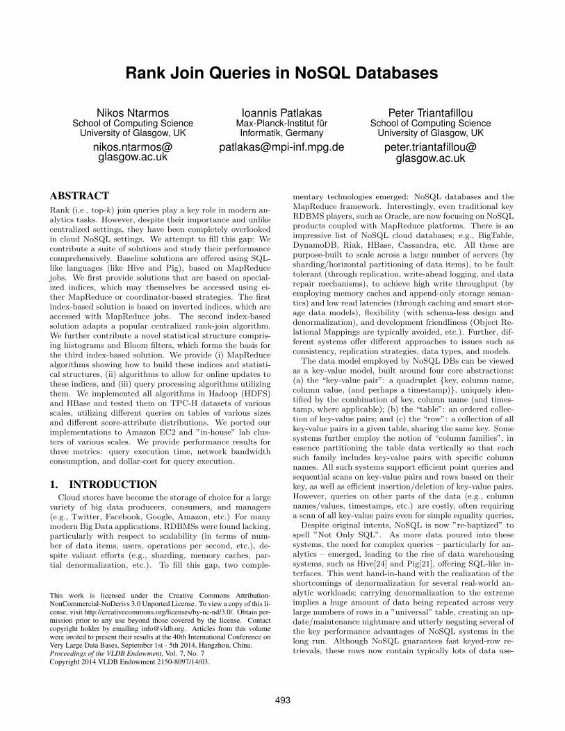
row join score row join scorekey value value key value valuer11 d 0.82 r21 a 0.51r12 c 0.93 r22 b 0.91r13 c 0.67 r23 c 0.64r14 d 0.82 r24 d 0.53r15 a 0.73 r25 d 0.41r16 c 0.79 r26 d 0.50r17 b 0.82 r27 a 0.35r18 b 0.70 r28 a 0.38r19 d 0.68 r29 a 0.37r110 a 1.00 r210 c 0.31r111 b 0.64 r211 b 0.92

Figure 1: Running example: Tuples of R1 and R2

to multi-way joins is straightforward. We first describe Hive’sand Pig’s approaches, as the baseline solutions for rank-joinqueries. Fig. 1 shows the input for our running example.

3.1 Rank Joins with Hive and PigIn Hive, rank join processing consists of two MapReduce

jobs plus a final stage. The first job computes and materi-alizes the join result set, while the second one computes thescore of the join result set tuples and stores them sorted ontheir score; a third, non-MapReduce stage then fetches thek highest-ranked results from the final list.

Pig takes a smarter approach. Its query plan optimizerpushes projections and top-k (STOP AFTER) operators asearly in the physical plan as possible, and takes extra mea-sures to better balance the load caused by the join result or-dering (ORDER BY) operator. Specifically, 3 MapReducejobs are used. The first computes the join result: mappersscan the table files, do early projections (stripping out un-related columns), and emit rows with the join value as theirkey; then, reducers group together rows with the same joinvalue, produce the join result set, and store it in an HDFSfile. The second MapReduce job is a by-product of the OR-DER BY clause; it samples the records in the join result filein the map phase, and appropriate quantiles are computedat the reduce phase. These quantiles are then used to con-struct a balanced partitioner for the third job, which ordersthe temporary records on their score and produces the top-kresult set. First, the map phase emits the temporary recordswith their join score as their key, and a combiners take overproducing a local top-k list. These lists are then assigned toa sole reducer producing the final top-k result set.

4. INDEXED RANK JOINSAs BigTable/HBase were the archetypical key-value cloud-

stores, we borrow their terminology in the description of thevarious algorithms and examples. It should be clear, though,that our indices and algorithms apply (perhaps with slight,obvious modifications) to all contemporary key-value stores.

4.1 Inverse Join List MapReduce Rank-JoinOur first algorithm – Inverse Join List MapReduce rank

join (IJLMR) – uses MapReduce, but utilizes an index toreduce the required MapReduce jobs to one, and avoid extranetwork transfers and inefficiencies.

4.1.1 IJLMR IndexIn the above approaches, the first stage mappers actually

create an inverted list of input tuples keyed by their join

Algorithm 1 IJLMR Index Creation

1 Input: Rows from a single column family (e.g., A), ofthe form {row.rowKey: row.joinValue, row.score}

2 Output: IJLMR index rows for A3 Map():4 foreach(row ∈ s e qu en t i a l scan o f A)5 emit(row.joinV alue: row.rowKey, row.score);

Row key Index tuples ({row key, score})(join value) R1 R2

a{r110 ,1.00}, {r15 ,0.73} {r21 ,0.51}, {r27 ,0.35},

{r28 ,0.38}, {r29 ,0.37}

b{r17 ,0.82}, {r18 ,0.70}, {r22 ,0.91}, {r211 ,0.92}{r111 ,0.64}

c{r12 ,0.93}, {r13 ,0.67}, {r23 ,0.64}, {r210 ,0.31}{r16 ,0.79}

d{r11 ,0.82}, {r14 ,0.82}, {r24 ,0.53}, {r25 ,0.41},{r19 ,0.68} {r26 ,0.50}

Figure 2: Running example: IJLMR index table

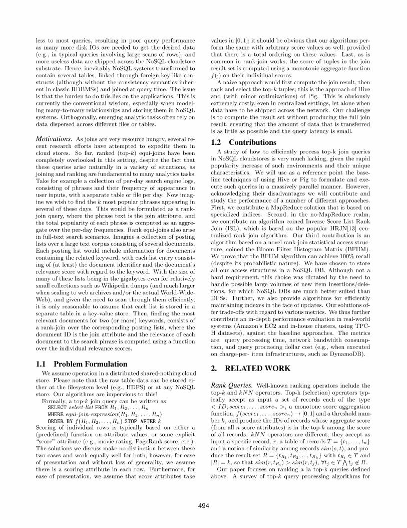
values; this is, in essence, a materialized view where eachentry has a join value as its key, and the input rows withthat specific join value as its set of values. Our IJLMRindex consists of a space-optimized form of these invertedlists, where index values consist of a list of tuples each beinga combination of the row key and score value of the indexedrow (Fig. 2). The IJLMR index for each indexed table isstored as a separate column family in one big table. Thismeans that, if the table is split up/sharded and distributedacross the NoSQL store nodes, index entries for the samejoin values across all indexed tables are stored next to eachother on the same node. The IJLMR index is built with amap-only MapReduce job (Algorithm 1) – a special type ofMapReduce job where there are no reducers and the outputof mappers is written directly into the NoSQL store. Wealso provide routines for online maintenance and updates tothis index, to be discussed shortly.

4.1.2 IJLMR Query ProcessingThe IJLMR query processing algorithm consists of a sin-

gle MapReduce job/stage, with several mappers and a sin-gle reducer (Algorithm 2). In this job, each mapper scansthrough its partition of the IJLMR index, reading columnsfrom the index column families for the joined tables, one rowat a time. For each row, it computes the Cartesian product(i.e., the join result) and join score of index entries from thedifferent column families; e.g., the mapper responsible forjoin value a (see Fig. 2) would produce 2× 4 key-values, themapper responsible for b would produce 3 × 2 tuples, etc.The mappers store in-memory only the top-k ranking resulttuples, and emit their final top-k list when their input data isexhausted. The single reducer then combines the individualtop-k lists and emits the global top-k result.

In addition to reducing the overall MapReduce jobs andstages down to one, this design has the added benefit thatdata transfers due to MapReduce shuffling/sorting are min-imized; the Hadoop framework ensures that each mapperis executed on the NoSQL store node storing its input re-gion data (or as close to it as possible), and thus only theindividual top-k result sets are transferred across the net-work and shuffled/sorted at the single reducer. As we shallsee in the performance evaluation section, this approach

496

Algorithm 2 IJLMR Rank-Join

1 Input: Rows from the IJLMR index for column families Aand B, of the form {row.joinValue: row.rowKey,row.score}

2 Output: Top-k join result set3 Map():4 foreach(row ∈ input) {5 HashTable tuplesA =∅, tuplesB =∅;6 Sor t edL i s t r e s u l t s =∅;7 foreach(kv ∈ row) {8 i f (kv.columnFamily == A) {9 myTuples = tuplesA . get (kv.joinV alue);

10 otherTuples = tuplesB . get (kv.joinV alue);11 } else {12 myTuples = tuplesB . get (kv.joinV alue);13 otherTuples = tuplesA . get (kv.joinV alue);14 }15 foreach (kv′ ∈ otherTuples ) {16 r e s u l t s .add( i nne rJo in (kv, kv′));17 r e s u l t s . tr im (k);18 }19 myTuples.append(kv.joinV alue, kv);20 }21 emit( r e s u l t s );22 Reduce():23 Sor t edL i s t r e s u l t s =∅;24 foreach(kv ∈ input) {25 r e s u l t s .add(kv);26 r e s u l t s . tr im (k);27 }28 emit( r e s u l t s ); // Final top -k result set

achieves at least an order of magnitude faster query process-ing times compared to Hive, and several orders of magnitudeless bandwidth consumption. Unfortunately, note that themappers still have to scan through the entire input dataset,weighing on the dollar-cost of query processing, which isalmost as high as that of the Hive approach.

4.2 Inverse Score List Rank-JoinClearly, network and disk I/O bandwidth savings are tan-

tamount. Also, taking advantage of the intrinsics of thequery processing engine of the NoSQL store at hand canprovide further improvements. We note that MapReduce isa poor match for such complex queries as top-k joins. Ourintuition is similar to that of Stonebraker, et al.[23], whopointed out that MapReduce is suboptimal for several as-pects of data management, including complex queries. Fol-lowing this thread of thought, we first overview HRJN[13]and then contribute Inverse Score List rank join (ISL).

4.2.1 HRJN OverviewAssume an n-way rank join between relations R1, R2, . . .,

Rn. In HRJN the tuples of each relation Ri are sorted inlists, ranked according to a scoring attribute Ri.score, orby using a scoring function on one or more attribute values.For simplicity, we assume the former scenario, but our solu-tions are equally applicable in the latter. The score of then-way join result tuples is then computed using a monotonicranking function f(R1.score, . . . , Rn.score) on the individ-ual scores of joined tuples. Tuples from the n lists are itera-tively retrieved in decreasing score order, and the algorithmkeeps the minimum (si) and maximum (si) tuple scores seenthus far (for i ∈ [1, . . . , n]). Every retrieved tuple is joinedagainst previously retrieved ones and appended to the result

Algorithm 3 ISL Index Creation

1 Input: Rows from a single column family (e.g., A), ofthe form {row.rowKey: row.joinValue, row.score}

2 Output: ISL index rows for A3 Map():4 foreach(row ∈ s e qu en t i a l scan o f A)5 emit(row.score: row.rowKey, row.joinvalue);

Row key(score)

Index tuples({row key, join value})R1 R2

-1.00 {r110 , a}-0.93 {r12 , c}-0.92 {r211 , b}-0.91 {r22 , b}-0.82 {r11 , d}, {r14 , d},

{r17 , b}-0.79 {r16 , c}

· · ·-0.35 {r27 , a}-0.31 {r210 , c}

Figure 3: Running example: ISL index table

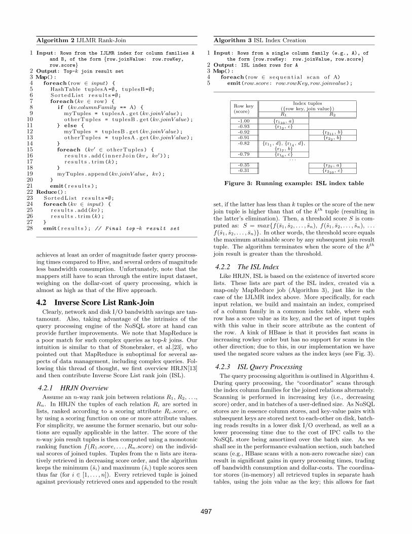
set, if the latter has less than k tuples or the score of the newjoin tuple is higher than that of the kth tuple (resulting inthe latter’s elimination). Then, a threshold score S is com-puted as: S = max{f(s1, s2, . . . , sn), f(s1, s2, . . . , sn), . . .f(s1, s2, . . . , sn)}. In other words, the threshold score equalsthe maximum attainable score by any subsequent join resulttuple. The algorithm terminates when the score of the kth

join result is greater than the threshold.

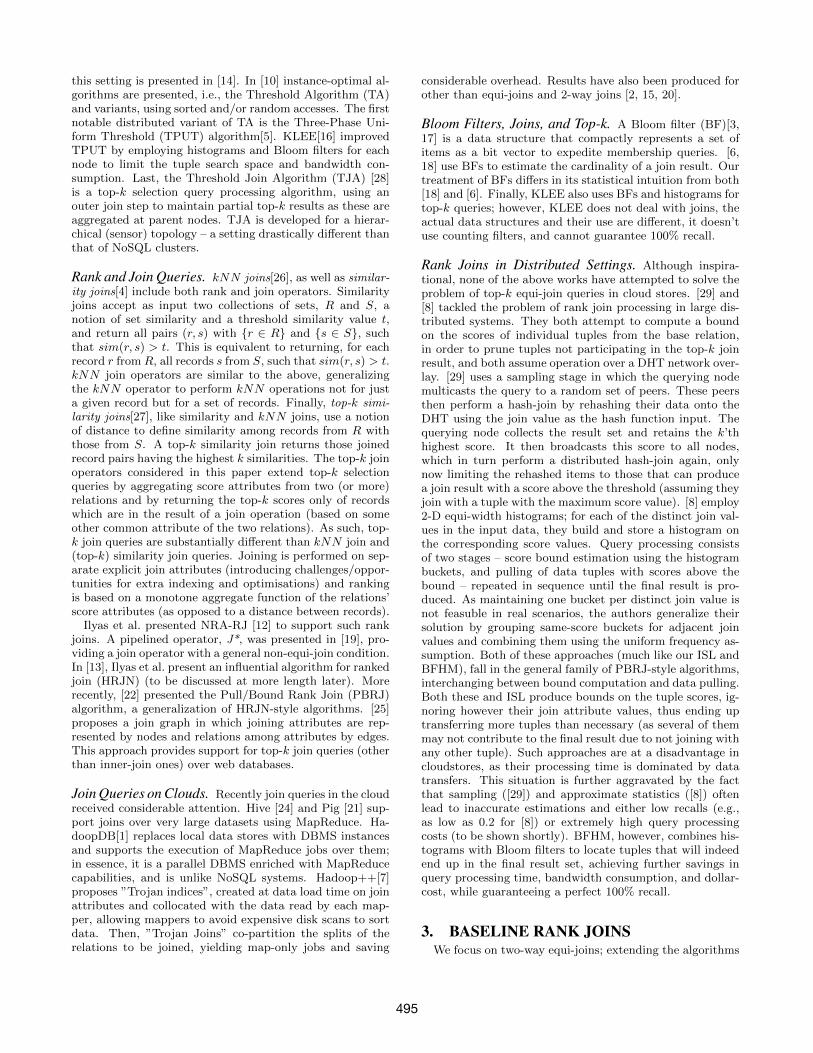
4.2.2 The ISL IndexLike HRJN, ISL is based on the existence of inverted score

lists. These lists are part of the ISL index, created via amap-only MapReduce job (Algorithm 3), just like in thecase of the IJLMR index above. More specifically, for eachinput relation, we build and maintain an index, comprisedof a column family in a common index table, where eachrow has a score value as its key, and the set of input tupleswith this value in their score attribute as the content ofthe row. A kink of HBase is that it provides fast scans inincreasing rowkey order but has no support for scans in theother direction; due to this, in our implementation we haveused the negated score values as the index keys (see Fig. 3).

4.2.3 ISL Query ProcessingThe query processing algorithm is outlined in Algorithm 4.

During query processing, the “coordinator” scans throughthe index column families for the joined relations alternately.Scanning is performed in increasing key (i.e., decreasingscore) order, and in batches of a user-defined size. As NoSQLstores are in essence column stores, and key-value pairs withsubsequent keys are stored next to each-other on disk, batch-ing reads results in a lower disk I/O overhead, as well as alower processing time due to the cost of IPC calls to theNoSQL store being amortized over the batch size. As weshall see in the performance evaluation section, such batchedscans (e.g., HBase scans with a non-zero rowcache size) canresult in significant gains in query processing times, tradingoff bandwidth consumption and dollar-costs. The coordina-tor stores (in-memory) all retrieved tuples in separate hashtables, using the join value as the key; this allows for fast

497

Algorithm 4 ISL Rank-Join

1 Input: Rows from the ISL index for column families Aand B, of the form {row.score: row.rowKey,row.joinvalue} (see Fig. 3), batch sizes CA, CB

2 Output: Top-k join result set3 HashTable tuplesA =∅, tuplesB =∅;4 Sor t edL i s t r e s u l t s =∅, batch=∅;5 CurrentRelat ion cr = A;6 while (true) {7 i f ( cr == A) {8 myTuples = tuplesA . get (kv.joinV alue);9 otherTuples = tuplesB . get (kv.joinV alue);

10 } else {11 myTuples = tuplesB . get (kv.joinV alue);12 otherTuples = tuplesA . get (kv.joinV alue);13 }14 batch. i n s e r t (next Ccr rows from CF "cr");15 foreach(row ∈ batch) {16 foreach(kv ∈ row) {17 myTuples.append(kv.joinV alue, kv);18 foreach (kv′ ∈ otherTuples ) {19 r e s u l t s .add( i nne rJo in (kv, kv′));20 i f (HRJNTerminationTest( r e s u l t s ,

tuplesA , tuplesB ) == true)21 return ( r e s u l t s );22 }23 }24 }25 batch. c l e a r ();26 cr = ( cr == A) ? B : A;27 }28 return ( r e s u l t s );

joins whenever new tuples are fetched. The coordinator fur-ther maintains a list of the current top-k results. With everynew tuple fetched and processed, the coordinator computesthe current threshold value, and terminates when it is belowthe score of the k’th tuple in the result set.

5. STATISTICAL RANK-JOINSBoth of the previous algorithms, ship tuples even though

they may not participate in the top-k result set. Our nextcontribution aims to avoid this. Note that we need not onlyestimate which tuples will produce the join result, but alsoto predict whether these tuples can have a top-k score.

5.1 The BFHM Data StructureThe BFHM index is a two-level statistical data structure,

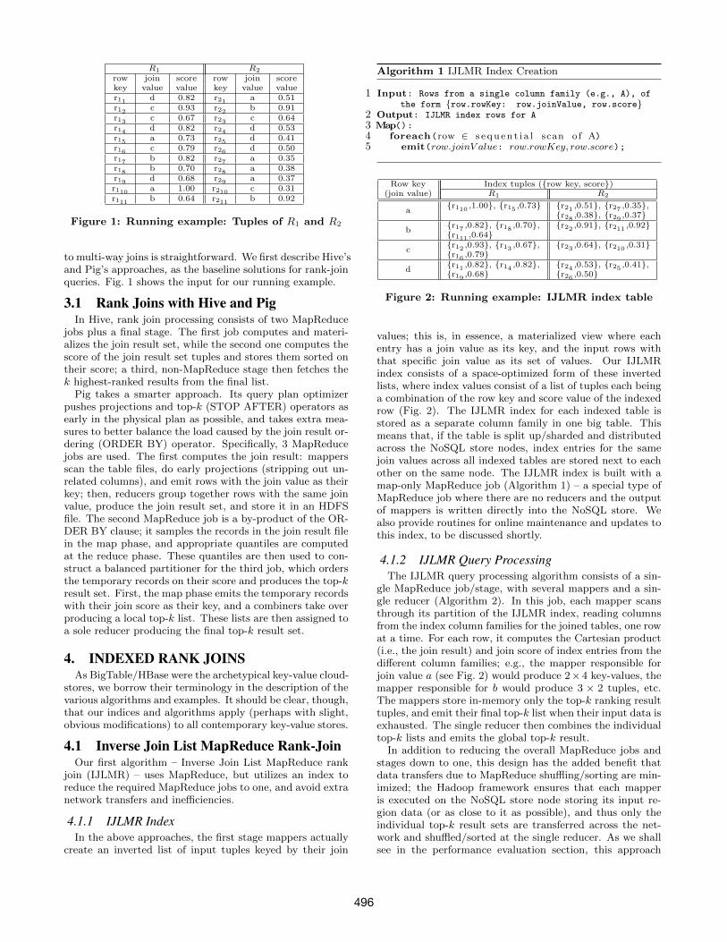
encompassing histograms and Bloom filters. At the firstlevel, we have an equi-width histogram on the score axis;that is, all histogram buckets have the same spread andeach such bucket stores information for tuples whose scoreslie within the boundaries of the bucket. At the second level,instead of a simple counter per bucket (plus the actual minand max scores of tuples recorded in the bucket), we chooseto maintain a Bloom filter-like data structure, recording thejoin values of the tuples belonging to the bucket. This willthen be used to estimate the cardinality of the join result setduring query processing, to be discussed shortly. In brief,the BFHM data structure has two main parameters: thenumber of buckets in the BFHM (numBuckets), and thenumber of bits in each BFHM bucket Bloom filter (m).

As false positives can inflate the join cardinality estima-tion, we have opted for a fusion scheme, combining single-hash-function Bloom filters with Counting Bloom filters and

Bitmap

...

0

1

0

0

1

0

1

0

Counters

(hash table)

1

2

1

r_1_8: b, 0.70

r_1_3: c, 0.67

r_1_9: d, 0.68

r_1_11: b, 0.64

Golomb compressed

h(b)

h(c)

h(b)

h(d)

Input data

Figure 4: BFHM bucket structure

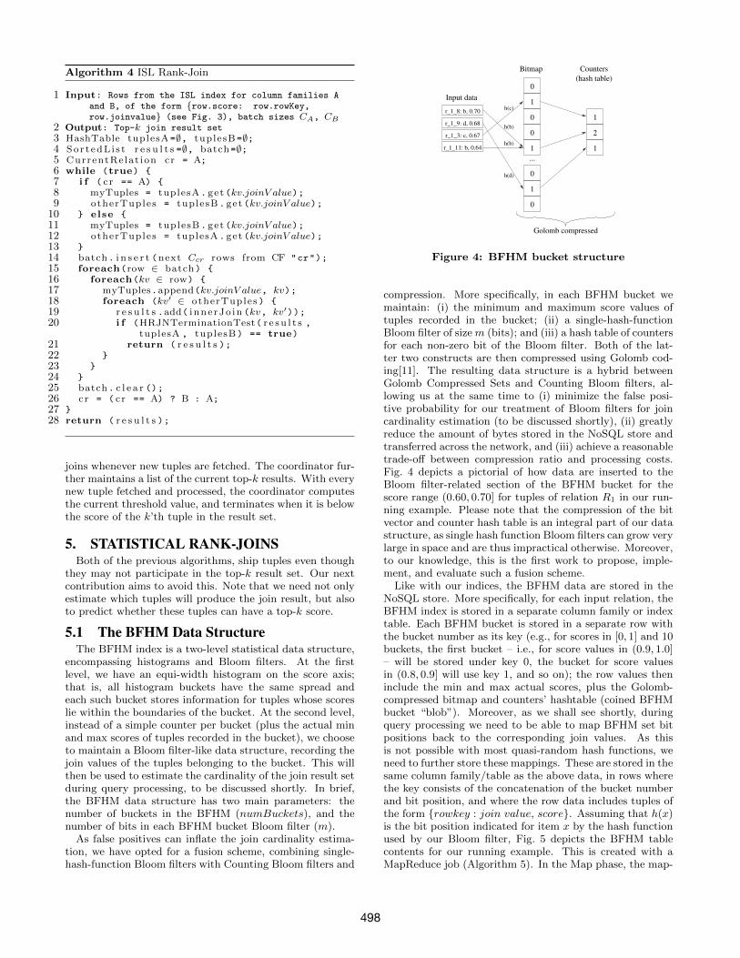
compression. More specifically, in each BFHM bucket wemaintain: (i) the minimum and maximum score values oftuples recorded in the bucket; (ii) a single-hash-functionBloom filter of sizem (bits); and (iii) a hash table of countersfor each non-zero bit of the Bloom filter. Both of the lat-ter two constructs are then compressed using Golomb cod-ing[11]. The resulting data structure is a hybrid betweenGolomb Compressed Sets and Counting Bloom filters, al-lowing us at the same time to (i) minimize the false posi-tive probability for our treatment of Bloom filters for joincardinality estimation (to be discussed shortly), (ii) greatlyreduce the amount of bytes stored in the NoSQL store andtransferred across the network, and (iii) achieve a reasonabletrade-off between compression ratio and processing costs.Fig. 4 depicts a pictorial of how data are inserted to theBloom filter-related section of the BFHM bucket for thescore range (0.60, 0.70] for tuples of relation R1 in our run-ning example. Please note that the compression of the bitvector and counter hash table is an integral part of our datastructure, as single hash function Bloom filters can grow verylarge in space and are thus impractical otherwise. Moreover,to our knowledge, this is the first work to propose, imple-ment, and evaluate such a fusion scheme.

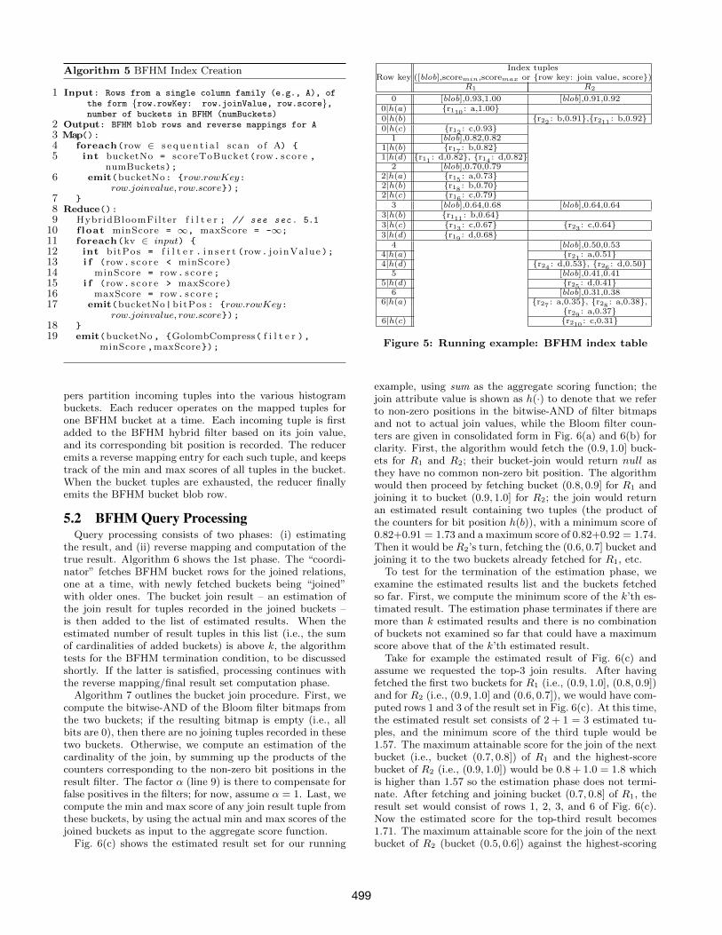
Like with our indices, the BFHM data are stored in theNoSQL store. More specifically, for each input relation, theBFHM index is stored in a separate column family or indextable. Each BFHM bucket is stored in a separate row withthe bucket number as its key (e.g., for scores in [0, 1] and 10buckets, the first bucket – i.e., for score values in (0.9, 1.0]– will be stored under key 0, the bucket for score valuesin (0.8, 0.9] will use key 1, and so on); the row values theninclude the min and max actual scores, plus the Golomb-compressed bitmap and counters’ hashtable (coined BFHMbucket “blob”). Moreover, as we shall see shortly, duringquery processing we need to be able to map BFHM set bitpositions back to the corresponding join values. As thisis not possible with most quasi-random hash functions, weneed to further store these mappings. These are stored in thesame column family/table as the above data, in rows wherethe key consists of the concatenation of the bucket numberand bit position, and where the row data includes tuples ofthe form {rowkey : join value, score}. Assuming that h(x)is the bit position indicated for item x by the hash functionused by our Bloom filter, Fig. 5 depicts the BFHM tablecontents for our running example. This is created with aMapReduce job (Algorithm 5). In the Map phase, the map-

498

Algorithm 5 BFHM Index Creation

1 Input: Rows from a single column family (e.g., A), ofthe form {row.rowKey: row.joinValue, row.score},number of buckets in BFHM (numBuckets)

2 Output: BFHM blob rows and reverse mappings for A3 Map():4 foreach(row ∈ s e qu en t i a l scan o f A) {5 int bucketNo = scoreToBucket(row. score ,

numBuckets);6 emit(bucketNo: {row.rowKey:

row.joinvalue, row.score});7 }8 Reduce():9 HybridBloomFilter f i l t e r ; // see sec. 5.1

10 f loat minScore = ∞, maxScore = -∞;11 foreach(kv ∈ input) {12 int bitPos = f i l t e r . i n s e r t (row. j o inValue );13 i f (row. s c o r e < minScore)14 minScore = row. s c o r e ;15 i f (row. s c o r e > maxScore)16 maxScore = row. s c o r e ;17 emit(bucketNo|bitPos : {row.rowKey:

row.joinvalue, row.score});18 }19 emit(bucketNo , {GolombCompress( f i l t e r ),

minScore ,maxScore});

pers partition incoming tuples into the various histogrambuckets. Each reducer operates on the mapped tuples forone BFHM bucket at a time. Each incoming tuple is firstadded to the BFHM hybrid filter based on its join value,and its corresponding bit position is recorded. The reduceremits a reverse mapping entry for each such tuple, and keepstrack of the min and max scores of all tuples in the bucket.When the bucket tuples are exhausted, the reducer finallyemits the BFHM bucket blob row.

5.2 BFHM Query ProcessingQuery processing consists of two phases: (i) estimating

the result, and (ii) reverse mapping and computation of thetrue result. Algorithm 6 shows the 1st phase. The “coordi-nator” fetches BFHM bucket rows for the joined relations,one at a time, with newly fetched buckets being “joined”with older ones. The bucket join result – an estimation ofthe join result for tuples recorded in the joined buckets –is then added to the list of estimated results. When theestimated number of result tuples in this list (i.e., the sumof cardinalities of added buckets) is above k, the algorithmtests for the BFHM termination condition, to be discussedshortly. If the latter is satisfied, processing continues withthe reverse mapping/final result set computation phase.

Algorithm 7 outlines the bucket join procedure. First, wecompute the bitwise-AND of the Bloom filter bitmaps fromthe two buckets; if the resulting bitmap is empty (i.e., allbits are 0), then there are no joining tuples recorded in thesetwo buckets. Otherwise, we compute an estimation of thecardinality of the join, by summing up the products of thecounters corresponding to the non-zero bit positions in theresult filter. The factor α (line 9) is there to compensate forfalse positives in the filters; for now, assume α = 1. Last, wecompute the min and max score of any join result tuple fromthese buckets, by using the actual min and max scores of thejoined buckets as input to the aggregate score function.

Fig. 6(c) shows the estimated result set for our running

Row keyIndex tuples

([blob],scoremin,scoremax or {row key: join value, score})R1 R2

0 [blob],0.93,1.00 [blob],0.91,0.920|h(a) {r110 : a,1.00}0|h(b) {r22 : b,0.91},{r211 : b,0.92}0|h(c) {r12 : c,0.93}

1 [blob],0.82,0.821|h(b) {r17 : b,0.82}1|h(d) {r11 : d,0.82}, {r14 : d,0.82}

2 [blob],0.70,0.792|h(a) {r15 : a,0.73}2|h(b) {r18 : b,0.70}2|h(c) {r16 : c,0.79}

3 [blob],0.64,0.68 [blob],0.64,0.643|h(b) {r111 : b,0.64}3|h(c) {r13 : c,0.67} {r23 : c,0.64}3|h(d) {r19 : d,0.68}

4 [blob],0.50,0.534|h(a) {r21 : a,0.51}4|h(d) {r24 : d,0.53}, {r26 : d,0.50}

5 [blob],0.41,0.415|h(d) {r25 : d,0.41}

6 [blob],0.31,0.386|h(a) {r27 : a,0.35}, {r28 : a,0.38},

{r29 : a,0.37}6|h(c) {r210 : c,0.31}

Figure 5: Running example: BFHM index table

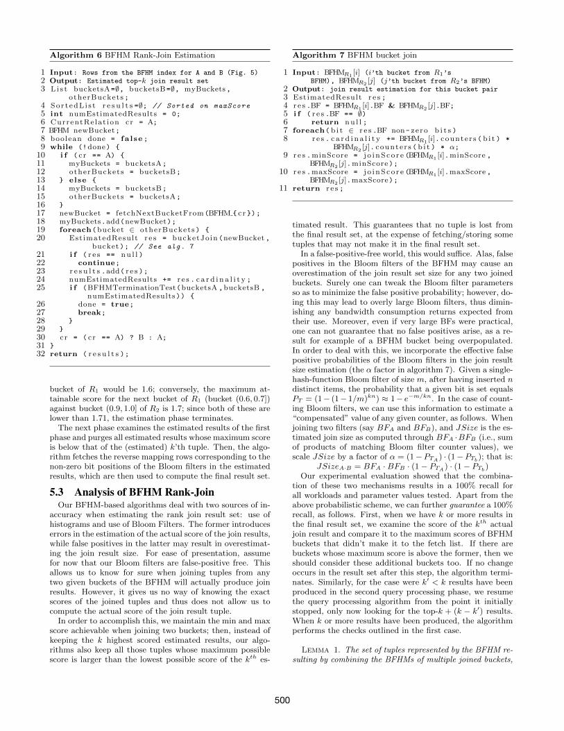
example, using sum as the aggregate scoring function; thejoin attribute value is shown as h(·) to denote that we referto non-zero positions in the bitwise-AND of filter bitmapsand not to actual join values, while the Bloom filter coun-ters are given in consolidated form in Fig. 6(a) and 6(b) forclarity. First, the algorithm would fetch the (0.9, 1.0] buck-ets for R1 and R2; their bucket-join would return null asthey have no common non-zero bit position. The algorithmwould then proceed by fetching bucket (0.8, 0.9] for R1 andjoining it to bucket (0.9, 1.0] for R2; the join would returnan estimated result containing two tuples (the product ofthe counters for bit position h(b)), with a minimum score of0.82+0.91 = 1.73 and a maximum score of 0.82+0.92 = 1.74.Then it would be R2’s turn, fetching the (0.6, 0.7] bucket andjoining it to the two buckets already fetched for R1, etc.

To test for the termination of the estimation phase, weexamine the estimated results list and the buckets fetchedso far. First, we compute the minimum score of the k’th es-timated result. The estimation phase terminates if there aremore than k estimated results and there is no combinationof buckets not examined so far that could have a maximumscore above that of the k’th estimated result.

Take for example the estimated result of Fig. 6(c) andassume we requested the top-3 join results. After havingfetched the first two buckets for R1 (i.e., (0.9, 1.0], (0.8, 0.9])and for R2 (i.e., (0.9, 1.0] and (0.6, 0.7]), we would have com-puted rows 1 and 3 of the result set in Fig. 6(c). At this time,the estimated result set consists of 2 + 1 = 3 estimated tu-ples, and the minimum score of the third tuple would be1.57. The maximum attainable score for the join of the nextbucket (i.e., bucket (0.7, 0.8]) of R1 and the highest-scorebucket of R2 (i.e., (0.9, 1.0]) would be 0.8 + 1.0 = 1.8 whichis higher than 1.57 so the estimation phase does not termi-nate. After fetching and joining bucket (0.7, 0.8] of R1, theresult set would consist of rows 1, 2, 3, and 6 of Fig. 6(c).Now the estimated score for the top-third result becomes1.71. The maximum attainable score for the join of the nextbucket of R2 (bucket (0.5, 0.6]) against the highest-scoring

499

Algorithm 6 BFHM Rank-Join Estimation

1 Input: Rows from the BFHM index for A and B (Fig. 5)2 Output: Estimated top-k join result set3 L i s t bucketsA=∅, bucketsB=∅, myBuckets ,

otherBuckets ;4 Sor t edL i s t r e s u l t s =∅; // Sorted on maxScore5 int numEstimatedResults = 0;6 CurrentRelat ion cr = A;7 BFHM newBucket;8 boolean done = fa l se ;9 while (!done) {

10 i f ( cr == A) {11 myBuckets = bucketsA;12 otherBuckets = bucketsB;13 } else {14 myBuckets = bucketsB;15 otherBuckets = bucketsA;16 }17 newBucket = fetchNextBucketFrom(BFHM { cr });18 myBuckets.add(newBucket);19 foreach(bucket ∈ otherBuckets ) {20 EstimatedResult r e s = bucketJoin (newBucket ,

bucket); // See alg. 721 i f ( r e s == nu l l )22 continue;23 r e s u l t s .add( r e s );24 numEstimatedResults += r e s . c a r d i n a l i t y ;25 i f (BFHMTerminationTest(bucketsA ,bucketsB ,

numEstimatedResults)) {26 done = true;27 break;28 }29 }30 cr = ( cr == A) ? B : A;31 }32 return ( r e s u l t s );

bucket of R1 would be 1.6; conversely, the maximum at-tainable score for the next bucket of R1 (bucket (0.6, 0.7])against bucket (0.9, 1.0] of R2 is 1.7; since both of these arelower than 1.71, the estimation phase terminates.

The next phase examines the estimated results of the firstphase and purges all estimated results whose maximum scoreis below that of the (estimated) k’th tuple. Then, the algo-rithm fetches the reverse mapping rows corresponding to thenon-zero bit positions of the Bloom filters in the estimatedresults, which are then used to compute the final result set.

5.3 Analysis of BFHM Rank-JoinOur BFHM-based algorithms deal with two sources of in-

accuracy when estimating the rank join result set: use ofhistograms and use of Bloom Filters. The former introduceserrors in the estimation of the actual score of the join results,while false positives in the latter may result in overestimat-ing the join result size. For ease of presentation, assumefor now that our Bloom filters are false-positive free. Thisallows us to know for sure when joining tuples from anytwo given buckets of the BFHM will actually produce joinresults. However, it gives us no way of knowing the exactscores of the joined tuples and thus does not allow us tocompute the actual score of the join result tuple.

In order to accomplish this, we maintain the min and maxscore achievable when joining two buckets; then, instead ofkeeping the k highest scored estimated results, our algo-rithms also keep all those tuples whose maximum possiblescore is larger than the lowest possible score of the kth es-

Algorithm 7 BFHM bucket join

1 Input: BFHMR1 [i] (i’th bucket from R1’sBFHM), BFHMR2

[j] (j’th bucket from R2’s BFHM)2 Output: join result estimation for this bucket pair3 EstimatedResult r e s ;4 r e s .BF = BFHMR1

[i].BF & BFHMR2[j].BF;

5 i f ( r e s .BF == ∅)6 return nu l l ;7 foreach( b i t ∈ r e s .BF non- zero b i t s )8 r e s . c a r d i n a l i t y += BFHMR1 [i]. counter s ( b i t ) *

BFHMR2[j]. counter s ( b i t ) * α;

9 r e s .minScore = j o i nS co r e (BFHMR1[i].minScore ,

BFHMR2 [j].minScore);10 r e s .maxScore = j o i nS co r e (BFHMR1

[i].maxScore ,BFHMR2

[j].maxScore);11 return r e s ;

timated result. This guarantees that no tuple is lost fromthe final result set, at the expense of fetching/storing sometuples that may not make it in the final result set.

In a false-positive-free world, this would suffice. Alas, falsepositives in the Bloom filters of the BFHM may cause anoverestimation of the join result set size for any two joinedbuckets. Surely one can tweak the Bloom filter parametersso as to minimize the false positive probability; however, do-ing this may lead to overly large Bloom filters, thus dimin-ishing any bandwidth consumption returns expected fromtheir use. Moreover, even if very large BFs were practical,one can not guarantee that no false positives arise, as a re-sult for example of a BFHM bucket being overpopulated.In order to deal with this, we incorporate the effective falsepositive probabilities of the Bloom filters in the join resultsize estimation (the α factor in algorithm 7). Given a single-hash-function Bloom filter of size m, after having inserted ndistinct items, the probability that a given bit is set equalsPT = (1− (1− 1/m)kn) ≈ 1− e−m/kn. In the case of count-ing Bloom filters, we can use this information to estimate a“compensated” value of any given counter, as follows. Whenjoining two filters (say BFA and BFB), and JSize is the es-timated join size as computed through BFA ·BFB (i.e., sumof products of matching Bloom filter counter values), wescale JSize by a factor of α = (1−PTA) · (1−PTb); that is:

JSizeA·B = BFA ·BFB · (1− PTA) · (1− PTb)Our experimental evaluation showed that the combina-

tion of these two mechanisms results in a 100% recall forall workloads and parameter values tested. Apart from theabove probabilistic scheme, we can further guarantee a 100%recall, as follows. First, when we have k or more results inthe final result set, we examine the score of the kth actualjoin result and compare it to the maximum scores of BFHMbuckets that didn’t make it to the fetch list. If there arebuckets whose maximum score is above the former, then weshould consider these additional buckets too. If no changeoccurs in the result set after this step, the algorithm termi-nates. Similarly, for the case were k′ < k results have beenproduced in the second query processing phase, we resumethe query processing algorithm from the point it initiallystopped, only now looking for the top-k + (k − k′) results.When k or more results have been produced, the algorithmperforms the checks outlined in the first case.

Lemma 1. The set of tuples represented by the BFHM re-sulting by combining the BFHMs of multiple joined buckets,

500

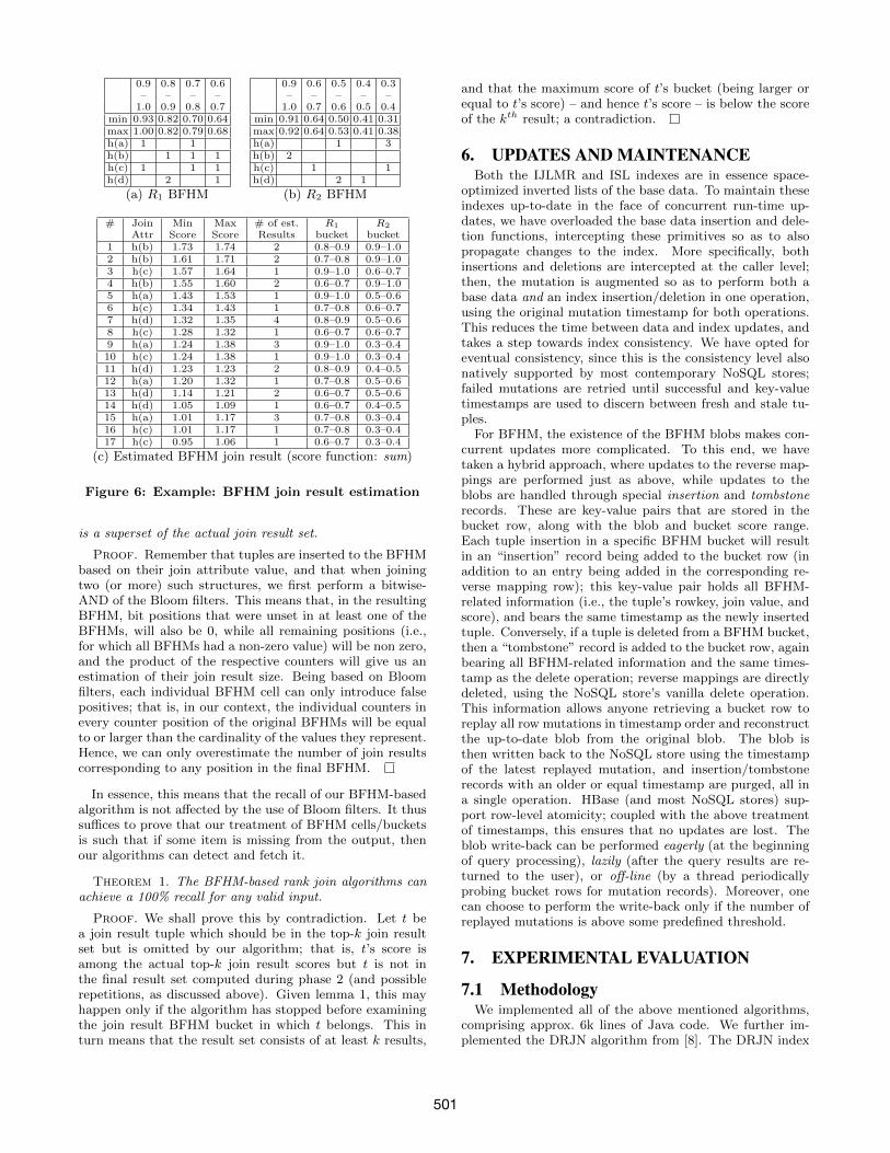
0.9 0.8 0.7 0.6– – – –1.0 0.9 0.8 0.7

min 0.93 0.82 0.70 0.64max 1.00 0.82 0.79 0.68h(a) 1 1h(b) 1 1 1h(c) 1 1 1h(d) 2 1

(a) R1 BFHM

0.9 0.6 0.5 0.4 0.3– – – – –1.0 0.7 0.6 0.5 0.4

min 0.91 0.64 0.50 0.41 0.31max 0.92 0.64 0.53 0.41 0.38h(a) 1 3h(b) 2h(c) 1 1h(d) 2 1

(b) R2 BFHM

# Join Min Max # of est. R1 R2

Attr Score Score Results bucket bucket1 h(b) 1.73 1.74 2 0.8–0.9 0.9–1.02 h(b) 1.61 1.71 2 0.7–0.8 0.9–1.03 h(c) 1.57 1.64 1 0.9–1.0 0.6–0.74 h(b) 1.55 1.60 2 0.6–0.7 0.9–1.05 h(a) 1.43 1.53 1 0.9–1.0 0.5–0.66 h(c) 1.34 1.43 1 0.7–0.8 0.6–0.77 h(d) 1.32 1.35 4 0.8–0.9 0.5–0.68 h(c) 1.28 1.32 1 0.6–0.7 0.6–0.79 h(a) 1.24 1.38 3 0.9–1.0 0.3–0.410 h(c) 1.24 1.38 1 0.9–1.0 0.3–0.411 h(d) 1.23 1.23 2 0.8–0.9 0.4–0.512 h(a) 1.20 1.32 1 0.7–0.8 0.5–0.613 h(d) 1.14 1.21 2 0.6–0.7 0.5–0.614 h(d) 1.05 1.09 1 0.6–0.7 0.4–0.515 h(a) 1.01 1.17 3 0.7–0.8 0.3–0.416 h(c) 1.01 1.17 1 0.7–0.8 0.3–0.417 h(c) 0.95 1.06 1 0.6–0.7 0.3–0.4

(c) Estimated BFHM join result (score function: sum)

Figure 6: Example: BFHM join result estimation

is a superset of the actual join result set.

Proof. Remember that tuples are inserted to the BFHMbased on their join attribute value, and that when joiningtwo (or more) such structures, we first perform a bitwise-AND of the Bloom filters. This means that, in the resultingBFHM, bit positions that were unset in at least one of theBFHMs, will also be 0, while all remaining positions (i.e.,for which all BFHMs had a non-zero value) will be non zero,and the product of the respective counters will give us anestimation of their join result size. Being based on Bloomfilters, each individual BFHM cell can only introduce falsepositives; that is, in our context, the individual counters inevery counter position of the original BFHMs will be equalto or larger than the cardinality of the values they represent.Hence, we can only overestimate the number of join resultscorresponding to any position in the final BFHM.

In essence, this means that the recall of our BFHM-basedalgorithm is not affected by the use of Bloom filters. It thussuffices to prove that our treatment of BFHM cells/bucketsis such that if some item is missing from the output, thenour algorithms can detect and fetch it.

Theorem 1. The BFHM-based rank join algorithms canachieve a 100% recall for any valid input.

Proof. We shall prove this by contradiction. Let t bea join result tuple which should be in the top-k join resultset but is omitted by our algorithm; that is, t’s score isamong the actual top-k join result scores but t is not inthe final result set computed during phase 2 (and possiblerepetitions, as discussed above). Given lemma 1, this mayhappen only if the algorithm has stopped before examiningthe join result BFHM bucket in which t belongs. This inturn means that the result set consists of at least k results,

and that the maximum score of t’s bucket (being larger orequal to t’s score) – and hence t’s score – is below the scoreof the kth result; a contradiction.

6. UPDATES AND MAINTENANCEBoth the IJLMR and ISL indexes are in essence space-

optimized inverted lists of the base data. To maintain theseindexes up-to-date in the face of concurrent run-time up-dates, we have overloaded the base data insertion and dele-tion functions, intercepting these primitives so as to alsopropagate changes to the index. More specifically, bothinsertions and deletions are intercepted at the caller level;then, the mutation is augmented so as to perform both abase data and an index insertion/deletion in one operation,using the original mutation timestamp for both operations.This reduces the time between data and index updates, andtakes a step towards index consistency. We have opted foreventual consistency, since this is the consistency level alsonatively supported by most contemporary NoSQL stores;failed mutations are retried until successful and key-valuetimestamps are used to discern between fresh and stale tu-ples.

For BFHM, the existence of the BFHM blobs makes con-current updates more complicated. To this end, we havetaken a hybrid approach, where updates to the reverse map-pings are performed just as above, while updates to theblobs are handled through special insertion and tombstonerecords. These are key-value pairs that are stored in thebucket row, along with the blob and bucket score range.Each tuple insertion in a specific BFHM bucket will resultin an “insertion” record being added to the bucket row (inaddition to an entry being added in the corresponding re-verse mapping row); this key-value pair holds all BFHM-related information (i.e., the tuple’s rowkey, join value, andscore), and bears the same timestamp as the newly insertedtuple. Conversely, if a tuple is deleted from a BFHM bucket,then a “tombstone” record is added to the bucket row, againbearing all BFHM-related information and the same times-tamp as the delete operation; reverse mappings are directlydeleted, using the NoSQL store’s vanilla delete operation.This information allows anyone retrieving a bucket row toreplay all row mutations in timestamp order and reconstructthe up-to-date blob from the original blob. The blob isthen written back to the NoSQL store using the timestampof the latest replayed mutation, and insertion/tombstonerecords with an older or equal timestamp are purged, all ina single operation. HBase (and most NoSQL stores) sup-port row-level atomicity; coupled with the above treatmentof timestamps, this ensures that no updates are lost. Theblob write-back can be performed eagerly (at the beginningof query processing), lazily (after the query results are re-turned to the user), or off-line (by a thread periodicallyprobing bucket rows for mutation records). Moreover, onecan choose to perform the write-back only if the number ofreplayed mutations is above some predefined threshold.

7. EXPERIMENTAL EVALUATION

7.1 MethodologyWe implemented all of the above mentioned algorithms,

comprising approx. 6k lines of Java code. We further im-plemented the DRJN algorithm from [8]. The DRJN index

501

is roughly a 2-d matrix, with join value partitions on its x-axis and score value partitions on its y-axis. DRJN queryprocessing proceeds as follows: (i) the querying node fetchescomplete DRJN matrix rows in decreasing score order; (ii)the relevant buckets are “joined” so as to estimate the car-dinality of their join; (iii) when the cumulative cardinalitysurpasses k, contact all nodes and fetch and join all tupleswhose score is above the the lower score boundaries of thelast fetched buckets; (iv) terminate if the cardinality of theactual result set is k and the score of the k’th tuple is largerthan the maximum attainable join score of the last fetchedbuckets, otherwise loop to (i), incrementally fetching morebuckets and tuples. As [8] was designed for a P2P-like set-ting, we had to revisit it so as to be useable in a NoSQL storesuch as HBase. First, we opted to group DRJN buckets bytheir scores and store all buckets for a given score range ascolumns of a single row; thus, the querying node will retrievea complete batch of buckets, as required at step (i) above,with a single HBase Get() operation. We further augmentedHBase with custom server-side filters to allow for efficient fil-tering of tuples in step (iv). Last, we further expedited step(iv) by implementing it as a lightweight Map-only Hadoopjob, storing its output data in a temporary HBase table forthe querying node to access and join.

We employed two different clusters: one in a controlledlab environment and one ”in-the-wild”. For the latter, weused Amazon’s Elastic Compute Cloud (EC2), with clustersconsisting of 3, 5, and 9 m1.large nodes. (each with 2 virtualcores, 7.5 GB RAM, and 2x 420 GB of instance storage).The lab cluster (LC) consisted of 5 nodes, each with 2 CPUs,16 cores per CPU, 64GB RAM, and 10× 1TB disks.

We used the TPC-H generator, generating data for the“Lineitem”, “Orders”, and ”Part” tables, for scale factorsfrom 10 to 500. The larger (smaller) data scale resulted intables with 3 billion (60M), 750 million (15M), and 100 mil-lion (2M) rows, which occupied ≈1.7TB (34GB), ≈200GB(4GB), and ≈25GB (0.5GB) of HBase disk space, respec-tively. With the TPC-H generator we also computed up-date sets, to be applied to the base data and indexes. AllBloom filters were configured to contain the most heavilypopulated of the buckets with a false positive probability of5%. The number of BFHM buckets was set to 100 and 1000on EC2 and to 100 and 500 on LC. ISL was configured withbatching sizes matching the number of BFHM buckets; 1%and 0.1% on EC2, and 1% and 0.2% on LC. DRJN was alsoconfigured with 100 and 500 buckets on LC.

We used the following queries:Q1: SELECT * FROM Part P, Lineitem L

WHERE P.PartKey=L.PartKeyORDER BY (P.RetailPrice * L.ExtendedPrice)STOP AFTER k

Q2: SELECT * FROM Orders O, Lineitem LWHERE O.OrderKey=L.OrderKeyORDER BY (O.TotalPrice + L.ExtendedPrice)STOP AFTER k

These queries were selected to showcase both the use ofdifferent aggregate scoring functions and the effect of scorevalue distributions on the query processing time. Querieswere executed 20 times and we report on the average values(the standard deviation was too small to show on the graphsin all cases). Last, we applied the update sets one at atime and executed 20 repetitions of the same queries. Allblock-level/memory caches were purged between consecutive

update and query executions.We evaluate all algorithms using the following metrics:• Turnaround time: the wall-clock time required to com-

pute and return the top-k join result.• Network bandwidth: the number of bytes transferred

through the network.• Dollar cost: the number of tuples read from the cloud

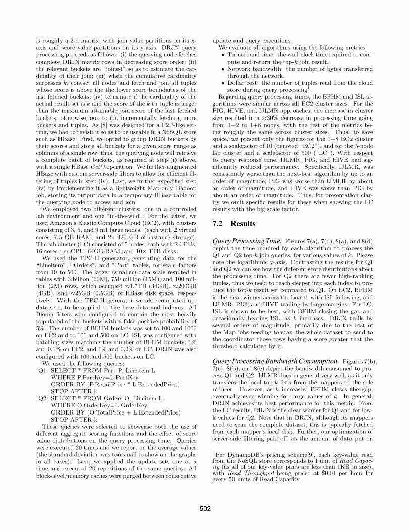
store during query processing1.Regarding query processing times, the BFHM and ISL al-

gorithms were similar across all EC2 cluster sizes. For thePIG, HIVE, and IJLMR approaches, the increase in clustersize resulted in a ≈30% decrease in processing time goingfrom 1+2 to 1+8 nodes, with the rest of the metrics be-ing roughly the same across cluster sizes. Thus, to savespace, we present only the figures for the 1+8 EC2 clusterand a scalefactor of 10 (denoted “EC2”), and for the 5-nodelab cluster and a scalefactor of 500 (“LC”). With respectto query response time, IJLMR, PIG, and HIVE had sig-nificantly reduced performance. Specifically, IJLMR, wasconsistently worse than the next-best algorithm by up to anorder of magnitude, PIG was worse than IJMLR by aboutan order of magnitude, and HIVE was worse than PIG byabout an order of magnitude. Thus, for presentation clar-ity we omit specific results for these when showing the LCresults with the big scale factor.

7.2 Results

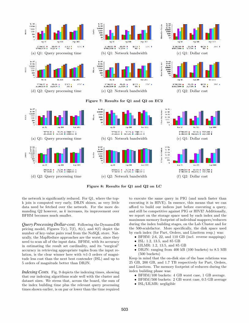
Query Processing Time. Figures 7(a), 7(d), 8(a), and 8(d)depict the time required by each algorithm to process theQ1 and Q2 top-k join queries, for various values of k. Pleasenote the logarithmic y-axis. Contrasting the results for Q1and Q2 we can see how the different score distributions affectthe processing time. For Q2 there are fewer high-rankingtuples, thus we need to reach deeper into each index to pro-duce the top-k result set compared to Q1. On EC2, BFHMis the clear winner across the board, with ISL following, andIJLMR, PIG, and HIVE trailing by large margins. For LC,ISL is shown to be best, with BFHM closing the gap andoccasionally beating ISL, as k increases. DRJN trails byseveral orders of magnitude, primarily due to the cost ofthe Map jobs needing to scan the whole dataset to send tothe coordinator those rows having a score greater that thethreshold calculated by it.

Query Processing Bandwidth Consumption. Figures 7(b),7(e), 8(b), and 8(e) depict the bandwidth consumed to pro-cess Q1 and Q2. IJLMR does in general very well, as it onlytransfers the local top-k lists from the mappers to the solereducer. However, as k increases, BFHM closes the gap,eventually even winning for large values of k. In general,DRJN achieves its best performance for this metric. Fromthe LC results, DRJN is the clear winner for Q1 and for low-k values for Q2. Note that in DRJN, although its mappersneed to scan the complete dataset, this is typically fetchedfrom each mapper’s local disk. Further, our optimization ofserver-side filtering paid off, as the amount of data put on

1Per DynamoDB’s pricing scheme[9], each key-value readfrom the NoSQL store corresponds to 1 unit of Read Capac-ity (as all of our key-value pairs are less than 1KB in size),with Read Throughput being priced at $0.01 per hour forevery 50 units of Read Capacity.

502

(a) Q1: Query processing time (b) Q1: Network bandwidth (c) Q1: Dollar cost

(d) Q2: Query processing time (e) Q2: Network bandwidth (f) Q2: Dollar cost

Figure 7: Results for Q1 and Q2 on EC2

(a) Q1: Query processing time (b) Q1: Network bandwidth (c) Q1: Dollar cost

(d) Q2: Query processing time (e) Q2: Network bandwidth (f) Q2: Dollar cost

Figure 8: Results for Q1 and Q2 on LC

the network is significantly reduced. For Q1, where the top-k join is computed very early, DRJN shines, as very littledata need be fetched over the network. For the more de-manding Q2 however, as k increases, its improvement overBFHM becomes much smaller.

Query Processing Dollar-cost. Following the DynamoDBpricing model, Figures 7(c), 7(f), 8(c), and 8(f) depict thenumber of key-value pairs read from the NoSQL store. Nat-urally, the MapReduce approaches are the worst, since theyneed to scan all of the input data. BFHM, with its accuracyin estimating the result set cardinality, and its “surgical”accuracy in retrieving appropriate tuples from the input re-lation, is the clear winner here with ≈1-3 orders of magni-tude less cost than the next best contender (ISL) and up to5 orders of magnitude better than DRJN.

Indexing Costs. Fig. 9 depicts the indexing times, showingthat our indexing algorithms scale well with the cluster anddataset sizes. We stress that, across the board, the sum ofthe index building time plus the relevant query processingtimes shown earlier, is on par or lower than the time required

to execute the same query in PIG (and much faster thanexecuting it in HIVE). In essence, this means that we canafford to build our indices just before executing a query,and still be competitive against PIG or HIVE! Additionally,we report on the storage space used by each index and themaximum memory footprint of individual mappers/reducersduring the index building stages, on the Lab Cluster and forthe 500-scalefactor. More specifically, the disk space usedby each index (for Part, Orders, and Lineitem resp.) was:• BFHM: 2.6, 22, and 110 GB (incl. reverse mappings)• ISL: 1.2, 13.5, and 85 GB• IJLMR: 1.2, 13.5, and 85 GB• DRJN: ranging from 400 kB (100 buckets) to 8.5 MB

(500 buckets)Keep in mind that the on-disk size of the base relations was25 GB, 200 GB, and 1.7 TB respectively for Part, Orders,and Lineitem. The memory footprint of reducers during theindex building phase was:• BFHM/100 buckets: 4 GB worst case, 1 GB average.• BFHM/500 buckets: 2 GB worst case, 0.5 GB average• ISL/IJLMR: negligible

503

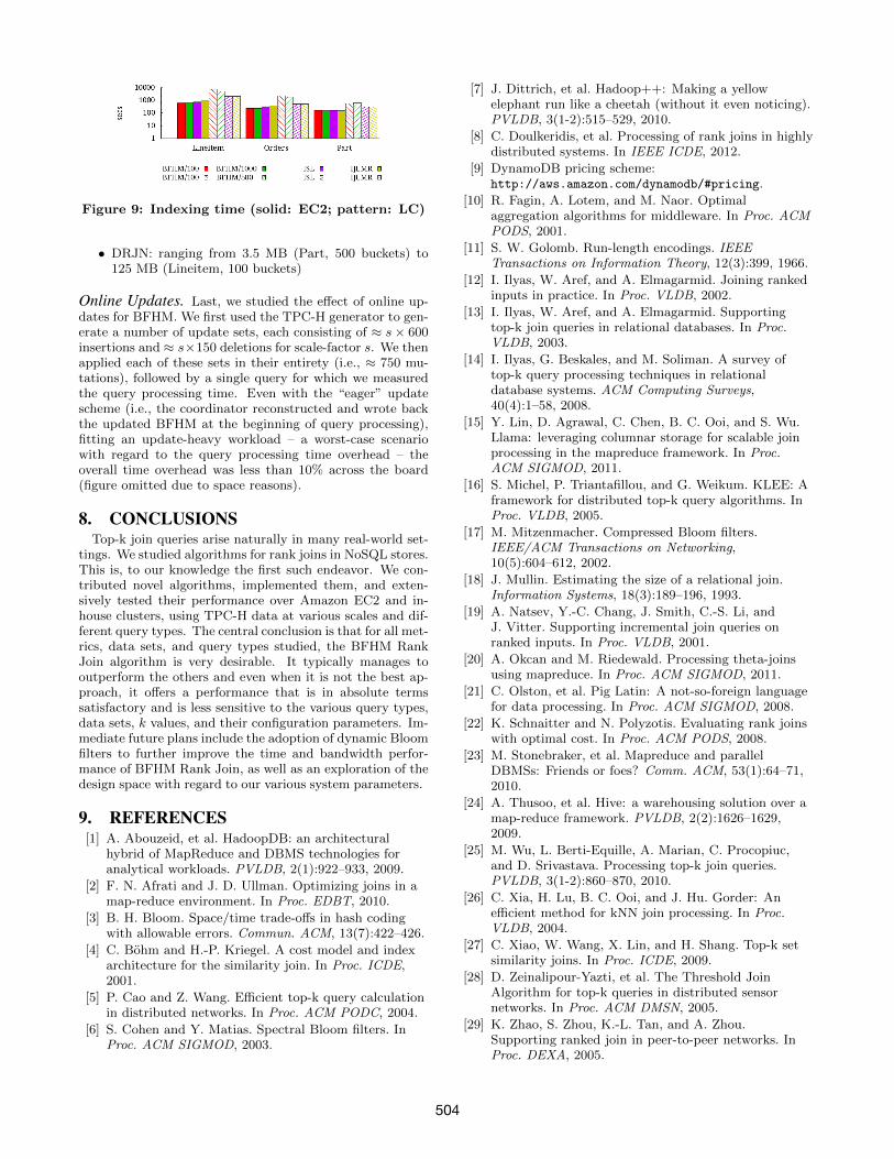
Figure 9: Indexing time (solid: EC2; pattern: LC)

• DRJN: ranging from 3.5 MB (Part, 500 buckets) to125 MB (Lineitem, 100 buckets)

Online Updates. Last, we studied the effect of online up-dates for BFHM. We first used the TPC-H generator to gen-erate a number of update sets, each consisting of ≈ s× 600insertions and ≈ s×150 deletions for scale-factor s. We thenapplied each of these sets in their entirety (i.e., ≈ 750 mu-tations), followed by a single query for which we measuredthe query processing time. Even with the “eager” updatescheme (i.e., the coordinator reconstructed and wrote backthe updated BFHM at the beginning of query processing),fitting an update-heavy workload – a worst-case scenariowith regard to the query processing time overhead – theoverall time overhead was less than 10% across the board(figure omitted due to space reasons).

8. CONCLUSIONSTop-k join queries arise naturally in many real-world set-

tings. We studied algorithms for rank joins in NoSQL stores.This is, to our knowledge the first such endeavor. We con-tributed novel algorithms, implemented them, and exten-sively tested their performance over Amazon EC2 and in-house clusters, using TPC-H data at various scales and dif-ferent query types. The central conclusion is that for all met-rics, data sets, and query types studied, the BFHM RankJoin algorithm is very desirable. It typically manages tooutperform the others and even when it is not the best ap-proach, it offers a performance that is in absolute termssatisfactory and is less sensitive to the various query types,data sets, k values, and their configuration parameters. Im-mediate future plans include the adoption of dynamic Bloomfilters to further improve the time and bandwidth perfor-mance of BFHM Rank Join, as well as an exploration of thedesign space with regard to our various system parameters.

9. REFERENCES[1] A. Abouzeid, et al. HadoopDB: an architectural

hybrid of MapReduce and DBMS technologies foranalytical workloads. PVLDB, 2(1):922–933, 2009.

[2] F. N. Afrati and J. D. Ullman. Optimizing joins in amap-reduce environment. In Proc. EDBT, 2010.

[3] B. H. Bloom. Space/time trade-offs in hash codingwith allowable errors. Commun. ACM, 13(7):422–426.

[4] C. Bohm and H.-P. Kriegel. A cost model and indexarchitecture for the similarity join. In Proc. ICDE,2001.

[5] P. Cao and Z. Wang. Efficient top-k query calculationin distributed networks. In Proc. ACM PODC, 2004.

[6] S. Cohen and Y. Matias. Spectral Bloom filters. InProc. ACM SIGMOD, 2003.

[7] J. Dittrich, et al. Hadoop++: Making a yellowelephant run like a cheetah (without it even noticing).PVLDB, 3(1-2):515–529, 2010.

[8] C. Doulkeridis, et al. Processing of rank joins in highlydistributed systems. In IEEE ICDE, 2012.

[9] DynamoDB pricing scheme:http://aws.amazon.com/dynamodb/#pricing.

[10] R. Fagin, A. Lotem, and M. Naor. Optimalaggregation algorithms for middleware. In Proc. ACMPODS, 2001.

[11] S. W. Golomb. Run-length encodings. IEEETransactions on Information Theory, 12(3):399, 1966.

[12] I. Ilyas, W. Aref, and A. Elmagarmid. Joining rankedinputs in practice. In Proc. VLDB, 2002.

[13] I. Ilyas, W. Aref, and A. Elmagarmid. Supportingtop-k join queries in relational databases. In Proc.VLDB, 2003.

[14] I. Ilyas, G. Beskales, and M. Soliman. A survey oftop-k query processing techniques in relationaldatabase systems. ACM Computing Surveys,40(4):1–58, 2008.

[15] Y. Lin, D. Agrawal, C. Chen, B. C. Ooi, and S. Wu.Llama: leveraging columnar storage for scalable joinprocessing in the mapreduce framework. In Proc.ACM SIGMOD, 2011.

[16] S. Michel, P. Triantafillou, and G. Weikum. KLEE: Aframework for distributed top-k query algorithms. InProc. VLDB, 2005.

[17] M. Mitzenmacher. Compressed Bloom filters.IEEE/ACM Transactions on Networking,10(5):604–612, 2002.

[18] J. Mullin. Estimating the size of a relational join.Information Systems, 18(3):189–196, 1993.

[19] A. Natsev, Y.-C. Chang, J. Smith, C.-S. Li, andJ. Vitter. Supporting incremental join queries onranked inputs. In Proc. VLDB, 2001.

[20] A. Okcan and M. Riedewald. Processing theta-joinsusing mapreduce. In Proc. ACM SIGMOD, 2011.

[21] C. Olston, et al. Pig Latin: A not-so-foreign languagefor data processing. In Proc. ACM SIGMOD, 2008.

[22] K. Schnaitter and N. Polyzotis. Evaluating rank joinswith optimal cost. In Proc. ACM PODS, 2008.

[23] M. Stonebraker, et al. Mapreduce and parallelDBMSs: Friends or foes? Comm. ACM, 53(1):64–71,2010.

[24] A. Thusoo, et al. Hive: a warehousing solution over amap-reduce framework. PVLDB, 2(2):1626–1629,2009.

[25] M. Wu, L. Berti-Equille, A. Marian, C. Procopiuc,and D. Srivastava. Processing top-k join queries.PVLDB, 3(1-2):860–870, 2010.

[26] C. Xia, H. Lu, B. C. Ooi, and J. Hu. Gorder: Anefficient method for kNN join processing. In Proc.VLDB, 2004.

[27] C. Xiao, W. Wang, X. Lin, and H. Shang. Top-k setsimilarity joins. In Proc. ICDE, 2009.

[28] D. Zeinalipour-Yazti, et al. The Threshold JoinAlgorithm for top-k queries in distributed sensornetworks. In Proc. ACM DMSN, 2005.

[29] K. Zhao, S. Zhou, K.-L. Tan, and A. Zhou.Supporting ranked join in peer-to-peer networks. InProc. DEXA, 2005.

504