RANDOMIZED SVD METHODS IN HYPERSPECTRALIMAGING

JIANI ZHANG, JENNIFER ERWAY, XIAOFEI HU, QIANG ZHANG,AND ROBERT PLEMMONS

Abstract. In this paper, we present a randomized singular value decomposition(rSVD) method for the purposes of lossless compression, reconstruction, classi-fication, and target detection with hyperspectral (HSI) data. Recent work inlow-rank matrix approximations obtained from random projections suggest thatthese approximations are well-suited for randomized dimensionality reduction.Approximation errors for the rSVD are evaluated on HSI and comparisons aremade to deterministic techniques and as well as to other randomized low-rankmatrix approximation methods involving compressive principal component anal-ysis. Numerical tests on real HSI data suggest that the method is promising, andis particularly effective for HSI data interrogation.

1. Introduction

Hyperspectral imagery (HSI) data are measurements of the electromagnetic radi-ation reflected from an object or scene (i.e., materials in the image) at many narrowwavelength bands. Often, this is represented visually as a cube, where each sliceof the cube represents the image at a different wavelength. Spectral information isimportant in many fields such as environmental remote sensing, monitoring chem-ical/oil spills, and military target discrimination. For comprehensive discussions,please see, e.g., [1, 2, 3]. Hyperspectral image data is often represented as a matrixA ∈ Rm×n, where each entry Aij is the reflection of ith pixel at the jth wavelength.Thus, a column of A contains the entire image at a given wavelength; each rowcontains the reflection of one pixel at all given wavelengths–often referred to as thespectral signature of a pixel.

HSI data can be collected over hundreds of wavelengths–creating truly massivedata sets. The transmission, storing, and processing of these large data sets oftenpresent significant difficulties in practical situations [1]. Dimensionality reductionmethods provide means to deal with the computational difficulties of the hyper-spectral data. These methods often use projections to compress a high-dimensionaldata space represented by a matrix A into a lower-dimensional space represented bya matrix B, which is then factorized. Such factorizations are referred to as low-rankmatrix factorizations, resulting in a low-rank matrix approximation to the originalHSI data matrix A. See, e.g., [2, 4, 5, 6].

Key words and phrases. random projections, hyperspectral imaging, dimension reduction, com-pressed sensing, singular value decomposition.

Research by Jiani Zhang and Jennifer Erway was supported by NSF grant DMS-08-11106.Research by Robert Plemmons and Qiang Zhang was supported by the U.S. Air Force Office

of Scientific Research (AFOSR), award number FA9550-11-1-0194, and by the U.S. NationalGeospatial-Intelligence Agency under Contract HM1582-10-C-0011, public release number PACase 12-433.

Corresponding author: Robert Plemmons, plemmons@wfu.edu, www.wfu.edu/˜plemmons.1

2 J. ZHANG, J. ERWAY, X. HU, Q. ZHANG, AND R. PLEMMONS

Dimensionality reduction techniques are generally regarded as lossy compression,i.e., the original data is not exactly represented or reconstructed by the lower-dimensional space. For lossless compression of HSI data, there have been effortsto exploit the correlation structure within HSI data plus coding the residuals afterstripping off the correlated parts, see e.g. [7, 8]. However, given the large num-ber of pixels, these correlations are often restricted to the spatially or spectrallylocal areas, while the dimension reduction techniques essentially explore the globalcorrelation structure. By coding the residuals after subtracting the original ma-trix by its low-dimensional representation, one can compress the original data in alossless manner, as in [8]. The success of lossless compression requires low entropyof the data distribution, and as we shall see in the experiments section, generallythe entropy of residuals for our method will be much lower than the entropy of theoriginal data.

Low-rank matrix factorizations can be computed using two general types of al-gorithms: deterministic and probabilistic. The most popular methods for deter-ministic low-rank factorizations include the singular value decomposition (SVD)[9] and principal component analysis (PCA) [10]. Advantages of these methodsinclude: first, often a small number of singular vectors (or principal components)sufficiently capture the action of a matrix; second, the singular vectors are orthonor-mal; third, the truncated SVD (TSVD) is the optimal low-rank representation ofthe original matrix in terms of Frobenius norm by the Eckart-Young Theorem [9].This last advantage is especially suited for compression with the TSVD method,since the Frobeniun norm of the residual matrix is the smallest among all rank-krepresentations of the original matrix, and hence we should expect a much lowerentropy in its distributions–make it suitable for compressive coding schemes. Bothdecompositions offer truncated versions so that these decompositions can be usedto represent an n-band hyperspectral image with the data-size-equivalent of onlyk images, where k n. For applications of the SVD and PCA in hyperspectralimaging see, e.g., [11, 12].

The traditional deterministic way of computing the SVD of a matrix A ∈ Rm×n

is typically a two-step procedure. In the first step, the matrix is reduced to abidiagonal matrix using Householder reflections or sometimes combined with a QRdecomposition if m n. This takes O(mn2) floating-point operations (flops),assuming that m ≥ n. The second step is to compute the SVD of the bidiagonalmatrix by an iterative method in O(n) iterations, each costing O(n) flops. Thus, theoverall cost is still O(mn2) flops [13, Lecture 31]. In HSI applications, the datasetscan easily break into the million-pixel or even giga-pixel level, which renders thisoperation impossible on typical desktop computers.

One solution is to apply probabilistic methods which give closely approximatedsingular vectors and singular values, while the complexity is at a much lower level.These methods begin by randomly projecting the original matrix to obtain a lower-dimensional matrix, while the range of the original matrix is asymptotically keptintact. The much-smaller projected matrix is then factorized using a full-matrixdecomposition such as SVD or PCA, after which the resulting singular vectors areback-projected to the original space. Compared to deterministic methods, prob-abilistic methods often offer the lower cost and more robustness in computation,while achieving high-accuracy results. See the seminal paper [14], and the referencestherein.

RANDOMIZED SVD METHODS IN HYPERSPECTRAL IMAGING 3

Knowing the redundancy of HSI data, especially in the spectral dimension, re-cently we have observed studies on the compressive HSI sensing, either algorithmic[11, 15] or experimental [6, 16, 17], and all of them involve a random projection ofthe data onto a lower-dimensional space. For example, in [11] Fowler proposed anapproach that exploits the use of compressive projections in sensors that integratedimensionality reduction and signal acquisition to effectively shift the computa-tional burden of PCA from the encoder platform to the decoder site. This tech-nique, termed Compressive-Projection PCA (CPPCA), couples random projectionsat the encoder with a Rayleigh-Ritz process for approximating eigenvectors at thedecoder. In its use of random projections, this technique can be considered topossess a certain duality with our approach to randomized SVD methods in HSI.However, CPPCA recovers coefficients of a known sparsity pattern in an unknownbasis. Accordingly, CPPCA requires the additional step of eigenvector recovery.

In this paper, we present a randomized singular value decomposition (rSVD)method for the purposes of lossless compression, reconstruction, classification andtarget detection. On a large HSI dataset we apply the rSVD method to demonstrateits efficiency and effectiveness of the proposed method. On another HSI dataset, wewill show the effectiveness of the proposed algorithm in detecting targets, especiallysmall targets, through singular vectors. In terms of reconstruction quality, we willcompare our algorithm with CPPCA [11] by using the signal-to-noise ratio (SNR).

We note that Chen, Nasrabadi and Tran [18] have recently provided an extensivestudy on the effects of linear projections on the performance of target detectionand classification of hyperspectral imagery. In their tests they found that thedimensionality of hyperspectral data can typically be reduced to 1/5 ∼ 1/3 that ofthe original data without severely affecting performance of commonly used targetdetection and classification algorithms.

The structure of the remainder of the paper is as follows. In Section 2, we givea detailed overview of rSVD in Section 2.1, the connections between this work andCPPCA in Section 2.2, and the compression and reconstruction of HSI data inSection 2.3. In Section 3, we present numerical results of the rSVD method on twopublicly available real data sets. Finally, we draw some conclusions and identifysome topics for future work in Section 4.

2. Review of Randomized Singular Value Decomposition

We start by defining terms and notations. The singular value decomposition(SVD) of a matrix A ∈ Rm×n is defined as

A = UΣV T , (1)

where U and V are orthonormal and Σ is a rectangular diagonal matrix whoseentries on the diagonal are the singular values denoted as σi. The column vectorsof U and V are left and right singular vectors, respectively, denoted as ui and vi.Define the truncated SVD (TSVD) approximation of A as a matrix Ak such that,

Ak =k∑

i=1

σiuivTi . (2)

We define the randomized SVD (rSVD) of A as,

Ak = UΣV T , (3)

4 J. ZHANG, J. ERWAY, X. HU, Q. ZHANG, AND R. PLEMMONS

where U and V are both orthonormal and Σ is diagonal with diagonal entriesdenoted as σi. Denote the column vectors of U and V as ui and vi respectively andcall them randomized singular vectors. Here, ui, vi and σi are related to ui, vi andσi, respectively. Define the residual matrix of a TSVD approximation as,

Rk = A− Ak, (4)

and the residual matrix of a rSVD approximation as,

Rk = A− Ak. (5)

Define the random projection of a matrix as,

Y = ΩTA, or Y = AΩ. (6)

where Ω is a random matrix with independent and identically distributed (i.i.d.)entries.

2.1. Randomized SVD Algorithm. The rSVD algorithm as considered by [14]explores approximate matrix factorizations using random projections, separatingthe process into two stages: In the first stage, random sampling is used to obtain areduced matrix whose range approximates the range of A; in the second stage, thereduced matrix is factorized. In this paper, we use this framework for computingthe rSVD of a matrix A.

The first stage of the method is common to many approximate matrix factor-ization methods: For a given ε > 0, we wish to find a matrix Q with orthonormalcolumns such that

‖A−QQTA‖2F ≤ ε. (7)The following algorithm [14] can be used to compute Q:

Input : An m× n matrix A and a precision measure ε.Output: An m× k matrix Q and rank k.Initialize Q as an empty matrix, e = 1 and k = 0.while e > ε do

1. k = k + 1.2. yi = Aωi, where ωi is a Gaussian random vector.3. qi =

(I −QQT

)yi.

4. qi = qi/‖qi‖.5. Q← [Q qi].6. Ω← [Ω ωi].7. Compute error e = ‖A−QQTA‖F/‖A‖F .

endAlgorithm 1: Construct an orthonormal matrix Q that approximates the rangeof matrix AΩ.

Because in practice we may not know the target rank k of A, Algorithm 1 allowsus to look for an appropriate target rank based upon given ε such that (7) holds.However if the target rank is known, one can avoid computing the error term e ateach iteration by replacing the While loop with a For loop. In practice, the numberof columns of Q is usually chosen to be slightly larger than the numerical rank of A[14]. Without loss of generality, we assume Q ∈ Rm×l, where l n. The columnsof Q form an orthogonal basis for the range of AΩ, where Ω is a matrix composed of

RANDOMIZED SVD METHODS IN HYPERSPECTRAL IMAGING 5

the random vectors wi, typically with a standard normal distribution [14]. Therange of the product AΩ is an approximation to the range of A.

The second stage of the rSVD method is to compute the SVD of the reducedmatrix QTA ∈ Rl×m. Since l n, it is generally computationally feasible tocompute the SVD of the reduced matrix. Letting UΣV T denote the SVD of QTA,we obtain:

A ≈ (QU)ΣV T = UΣV T , (8)where U = QU and V are orthogonal matrices, and thus by (8), UΣV T is anapproximate SVD of A and the range of U is an approximation to range of A.Algorithm 2 summarizes the discussion above. See [14] for details on the choice ofl, along with extensive numerical experiments using randomized SVD methods anda detailed error analysis of the two-stage method described above.

Input : An m× n matrix A, and rank k with k ≤ n ≤ m.Output: The rSVD of A: U , Σ, V .1. Generate a Gaussian random matrix Ω ∈ Rn×k.2. Form the projection of A: Y = AΩ.3. Construct Q ∈ Rm×k by Algorithm 1.4. Set B = QTA ∈ Rk×n.5. Compute the SVD of B, B = UΣV T .6. U = QU .

Algorithm 2: The basic rSVD algorithm

Next we discuss several variations of Algorithm 2 depending on the properties ofA. We will test all cases in the numerical results section.Case 1. If knowing the target rank k, and if the singular values of A decay

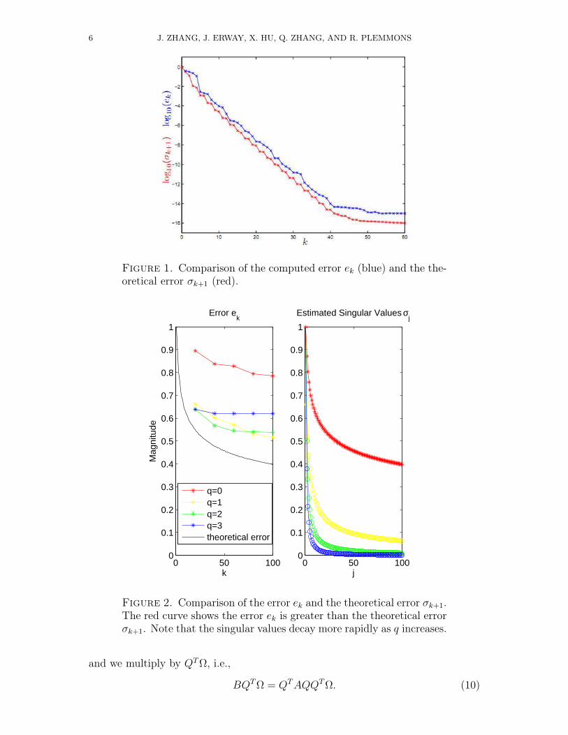
rapidly, we can skip Algorithm 1 by simply using the rank revealing QR factoriza-tion, Y = QR, where Q is an orthogonal basis of the range of Y . Figure 1 from [19]compares the approximation error ek and the theoretical error σk+1 of a matrix A,and clearly when the singular values of A decay rapidly, ek is close to the theoreticalerror σk+1 with high probability.Case 2. If the singular values of A decay gradually, or σk/σ1 is not small, we

may lose the accuracy of estimates. Consider introducing a power q and forming Yas Y = (AAT )qAR. Since (AAT )qΩ has the same singular vectors as A, while itssingular values, σ2q−1

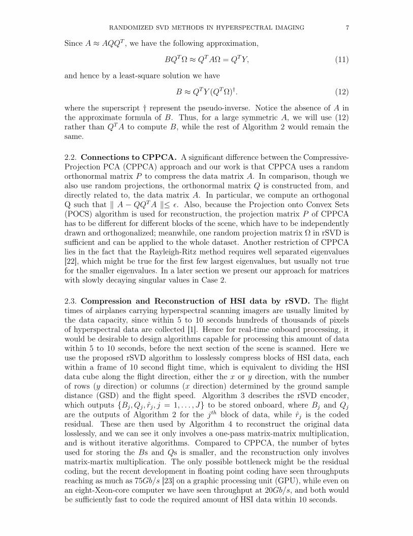
i , i = 1, . . . , n, decay more rapidly. Hence the error will besmaller by Theorem 2.3 and Theorem 2.5 in [14]. From Figure 2, we see the ek isnot always close to σk+1, especially when q = 0, but by increasing the power q, weobserve the reduction of errors.Case 3. Algorithm 2 requires us to revisit the input matrix, while this may be

not feasible for large matrices. For example, in ultraspectral imaging [20], one couldhave thousands of spectral bands, and PCA on such datasets would require comput-ing the eigenvectors and eigenvalues of a covariance matrix with a huge dimension.Another example is in the atmospheric correction model called MODTRAN5 [21],that utilizes large lookup tables (LUT), and the compression of LUTs by the PCAtechnique would again require the eigen decomposition of large covariance matrices.Here we introduce a variation of Algorithm 2 that only requires one pass over alarge symmetric matrix. Now we define matrix B as

B = QTAQ, (9)

6 J. ZHANG, J. ERWAY, X. HU, Q. ZHANG, AND R. PLEMMONS

Figure 1. Comparison of the computed error ek (blue) and the the-oretical error σk+1 (red).

0 50 1000

0.1

0.2

0.3

0.4

0.5

0.6

0.7

0.8

0.9

1

Estimated Singular Values σj

j0 50 100

0

0.1

0.2

0.3

0.4

0.5

0.6

0.7

0.8

0.9

1

Error ek

Mag

nitu

de

k

q=0q=1q=2q=3theoretical error

Figure 2. Comparison of the error ek and the theoretical error σk+1.The red curve shows the error ek is greater than the theoretical errorσk+1. Note that the singular values decay more rapidly as q increases.

and we multiply by QTΩ, i.e.,

BQTΩ = QTAQQTΩ. (10)

RANDOMIZED SVD METHODS IN HYPERSPECTRAL IMAGING 7

Since A ≈ AQQT , we have the following approximation,

BQTΩ ≈ QTAΩ = QTY, (11)

and hence by a least-square solution we have

B ≈ QTY (QTΩ)†. (12)

where the superscript † represent the pseudo-inverse. Notice the absence of A inthe approximate formula of B. Thus, for a large symmetric A, we will use (12)rather than QTA to compute B, while the rest of Algorithm 2 would remain thesame.

2.2. Connections to CPPCA. A significant difference between the Compressive-Projection PCA (CPPCA) approach and our work is that CPPCA uses a randomorthonormal matrix P to compress the data matrix A. In comparison, though wealso use random projections, the orthonormal matrix Q is constructed from, anddirectly related to, the data matrix A. In particular, we compute an orthogonalQ such that ‖ A − QQTA ‖≤ ε. Also, because the Projection onto Convex Sets(POCS) algorithm is used for reconstruction, the projection matrix P of CPPCAhas to be different for different blocks of the scene, which have to be independentlydrawn and orthogonalized; meanwhile, one random projection matrix Ω in rSVD issufficient and can be applied to the whole dataset. Another restriction of CPPCAlies in the fact that the Rayleigh-Ritz method requires well separated eigenvalues[22], which might be true for the first few largest eigenvalues, but usually not truefor the smaller eigenvalues. In a later section we present our approach for matriceswith slowly decaying singular values in Case 2.

2.3. Compression and Reconstruction of HSI data by rSVD. The flighttimes of airplanes carrying hyperspectral scanning imagers are usually limited bythe data capacity, since within 5 to 10 seconds hundreds of thousands of pixelsof hyperspectral data are collected [1]. Hence for real-time onboard processing, itwould be desirable to design algorithms capable for processing this amount of datawithin 5 to 10 seconds, before the next section of the scene is scanned. Here weuse the proposed rSVD algorithm to losslessly compress blocks of HSI data, eachwithin a frame of 10 second flight time, which is equivalent to dividing the HSIdata cube along the flight direction, either the x or y direction, with the numberof rows (y direction) or columns (x direction) determined by the ground sampledistance (GSD) and the flight speed. Algorithm 3 describes the rSVD encoder,which outputs Bj, Qj, rj, j = 1, . . . , J to be stored onboard, where Bj and Qj

are the outputs of Algorithm 2 for the jth block of data, while rj is the codedresidual. These are then used by Algorithm 4 to reconstruct the original datalosslessly, and we can see it only involves a one-pass matrix-matrix multiplication,and is without iterative algorithms. Compared to CPPCA, the number of bytesused for storing the Bs and Qs is smaller, and the reconstruction only involvesmatrix-martix multiplication. The only possible bottleneck might be the residualcoding, but the recent development in floating point coding have seen throughputsreaching as much as 75Gb/s [23] on a graphic processing unit (GPU), while even onan eight-Xeon-core computer we have seen throughput at 20Gb/s, and both wouldbe sufficiently fast to code the required amount of HSI data within 10 seconds.

8 J. ZHANG, J. ERWAY, X. HU, Q. ZHANG, AND R. PLEMMONS

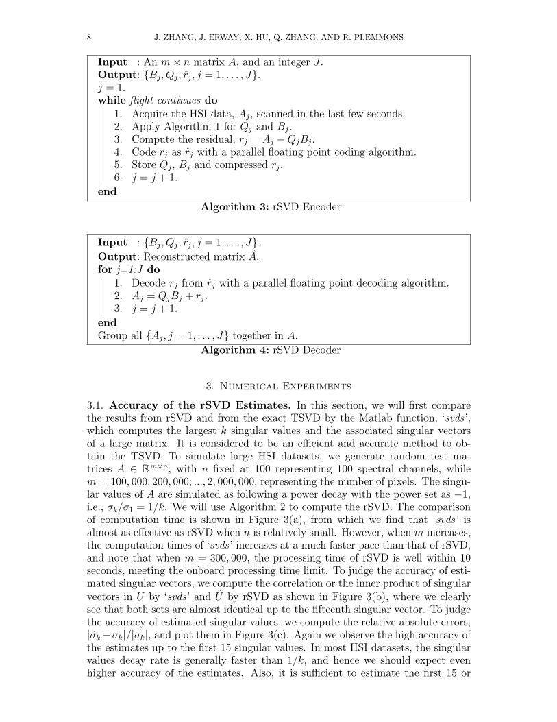
Input : An m× n matrix A, and an integer J .Output: Bj, Qj, rj, j = 1, . . . , J.j = 1.while flight continues do

1. Acquire the HSI data, Aj, scanned in the last few seconds.2. Apply Algorithm 1 for Qj and Bj.3. Compute the residual, rj = Aj −QjBj.4. Code rj as rj with a parallel floating point coding algorithm.5. Store Qj, Bj and compressed rj.6. j = j + 1.

endAlgorithm 3: rSVD Encoder

Input : Bj, Qj, rj, j = 1, . . . , J.Output: Reconstructed matrix A.for j=1:J do

1. Decode rj from rj with a parallel floating point decoding algorithm.2. Aj = QjBj + rj.3. j = j + 1.

endGroup all Aj, j = 1, . . . , J together in A.

Algorithm 4: rSVD Decoder

3. Numerical Experiments

3.1. Accuracy of the rSVD Estimates. In this section, we will first comparethe results from rSVD and from the exact TSVD by the Matlab function, ‘svds ’,which computes the largest k singular values and the associated singular vectorsof a large matrix. It is considered to be an efficient and accurate method to ob-tain the TSVD. To simulate large HSI datasets, we generate random test ma-trices A ∈ Rm×n, with n fixed at 100 representing 100 spectral channels, whilem = 100, 000; 200, 000; ..., 2, 000, 000, representing the number of pixels. The singu-lar values of A are simulated as following a power decay with the power set as −1,i.e., σk/σ1 = 1/k. We will use Algorithm 2 to compute the rSVD. The comparisonof computation time is shown in Figure 3(a), from which we find that ‘svds ’ isalmost as effective as rSVD when n is relatively small. However, when m increases,the computation times of ‘svds ’ increases at a much faster pace than that of rSVD,and note that when m = 300, 000, the processing time of rSVD is well within 10seconds, meeting the onboard processing time limit. To judge the accuracy of esti-mated singular vectors, we compute the correlation or the inner product of singularvectors in U by ‘svds ’ and U by rSVD as shown in Figure 3(b), where we clearlysee that both sets are almost identical up to the fifteenth singular vector. To judgethe accuracy of estimated singular values, we compute the relative absolute errors,|σk−σk|/|σk|, and plot them in Figure 3(c). Again we observe the high accuracy ofthe estimates up to the first 15 singular values. In most HSI datasets, the singularvalues decay rate is generally faster than 1/k, and hence we should expect evenhigher accuracy of the estimates. Also, it is sufficient to estimate the first 15 or

RANDOMIZED SVD METHODS IN HYPERSPECTRAL IMAGING 9

0 0.5 1 1.5 2

x 106

0

50

100

150

200

250

m

seco

nds

0 5 10 15 200.4

0.6

0.8

1

1.2

k

corr

elat

ion

0 5 10 15 200

0.02

0.04

0.06

0.08

k

rela

tive

abso

lute

err

or

svdsrSVD

Figure 3. (a) Computation time of ‘svds ’ and rSVD. (b) Corre-lations between the singular vectors in U by ‘svds ’ and rSVD. (c)Relative absolute differences between the singular values estimatedby ‘svds ’ and rSVD.

0 10 20 30 40 50 60 70 80 90 10010

−20

10−15

10−10

10−5

100

105

ith largest singular value

sing

ular

val

ue

100 largest singular values of a Toeplitz matrix

Figure 4. Illustration rapidly decaying singular values of matrix ofsize 1000× 1000.

even 10 singular vectors and singular values, which would often cover more than90% of the original variance of the HSI data [1].

Then we numerically test the three special cases discussed in Section 2.1.Case 1. We have considered square Toeplitz matrices with increasingly large

sizes, n = 15, 30, ..., 1500. Figure 4 shows the rapid decay of a 1, 000×1, 000 matrixand hence they are suitable for testing the algorithm. Figure 5(a) shows that therelative Frobenius norm errors rise and fall in the order of 10−12, and remain inthe same order even when the size of a matrix increase. Figure 5(b) demonstratesthat the computational time of rSVD is very short for the Toeplitz matrices whosesingular values decay rapidly.Case 2. Here we simulate 10, 000× 100 matrices with slowly decaying singular

values, i.e., σi/σ1 = i−s, with s = 0.2, 0.4, . . . , 1.0. For each matrix, we run therSVD algorithm 100 times for each power q in the set, q = 1, 2, . . . , 20. Thenorm errors of reconstructed matrices are averaged across 100 runs and normalized

10 J. ZHANG, J. ERWAY, X. HU, Q. ZHANG, AND R. PLEMMONS

0 500 1000 15000

1

2

3

4

5x 10

−12

the size of matrices (n by n)

rela

tive

erro

r

(a)

0 500 1000 15000

0.5

1

1.5

2

the size of matrices (n by n)

seco

nds

(b)

Figure 5. (a) The relative errors between the rSVD low-rank ap-proximation and the original matrix A are shown by the red curve.(b) The computational time for rSVD.

by the norm error when q = 1, i.e., eq/e1. Figure 6 shows that increasing the power qimproves the reconstruction quality or decreases the norm error, and greater effectsare observed for larger s, because the singular values of (AAT )q are σ2q

i = σ2q1 i−2qs.

Case 3. To simulate covariance matrices, we generate a sequence of positivedefinite symmetric matrices with increasing size as n = 100, 110, . . . , 2, 000. Theeigen-spectrum follows a power decay with the power set as −1. We apply themodified B as in Case 3 to compute its SVD, rather than using QTA. We setk = 25. Figure 7(a) shows the computation time compared with using regular SVDin MATLAB, while Figure 7(b) shows the relative Frobenius norm errors betweenthe original matrix and its low-rank approximation. Apparently the computationtime used by rSVD is far less than the regular SVD, while the accuracies are quitehigh.

3.2. rSVD on a large HSI dataset and a lossless compression. The rSVDalgorithm was also applied to a relatively large HSI dataset consisting of a 920 ×4, 933× 58 image cube collected over Gulfport MS by a commercial hyperspectralsensor having a spectral range of 0.45 to 0.72 microns. This cube was then unfoldedinto a large matrix of size 4,538,360 x 58. Running an exact SVD algorithm is almostimpossible on a regular desktop computer with limited memory and speed, while

RANDOMIZED SVD METHODS IN HYPERSPECTRAL IMAGING 11

0 5 10 15 200.75

0.8

0.85

0.9

0.95

1

q

e q/e1

s=.2s=.4s=.6s=.8s=1.0

Figure 6. The reduction of norm error by increasing the power qfor singular value spectrums decaying with various powers s.

0 500 1000 1500 200010

−4

10−3

10−2

10−1

100

n

seco

nds

(a)

0 500 1000 1500 20000.13

0.14

0.15

0.16

0.17

0.18

0.19

n

norm

err

or(b)

rSVDSVD

Figure 7. (a) Computation time of rSVD in blue and SVD in green.(b) Relative norm errors by rSVD and SVD.

the rSVD algorithm gives us singular values and vectors very close to the true ones,with a significantly reduced amount of flops and memory required. For the first 25singular vectors and singular values, it only takes 68 seconds on a desktop computerwith Xeon 3.2 GHz Quadcores and 12 GB memory. From the computed singularvalues and vectors, we observed that the singular vectors after the ninth singularvector all appear to be noise, indicating that the data matrix does have a low-rankrepresentation.

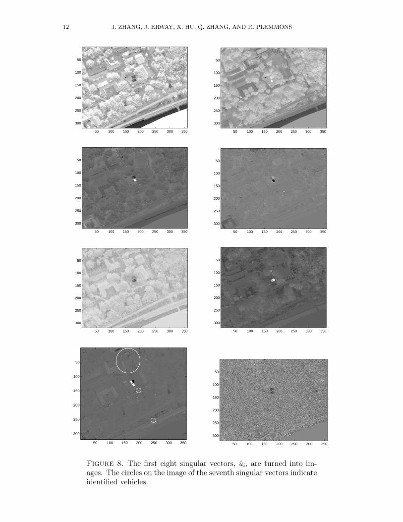
Figure 8 shows the results for a small scene from the large dataset describedabove, consisting of part of the University of Southern Mississippi Campus, ex-tracted from the large Gulfport MS dataset. Notice the targets placed in the scene,for detection and identification tests. The first eight singular vectors, ui, are foldedback from the transformed data. The first singular vector shown in Figure 8 is themean image across 58 spectral bands, while the second singular vector shows highintensity at the grass and foliage pixels, the third shows the targets quite clearly, aswell as high reflectance sandy areas or rooftops, the fifth shows the low reflectancepavement or roof tops, and shadows and the seventh shows vehicles at various placesmarked by the circles. Starting from the eighth, the rest of the singular vectorsappear to be mostly noise.

12 J. ZHANG, J. ERWAY, X. HU, Q. ZHANG, AND R. PLEMMONS

50 100 150 200 250 300 350

50

100

150

200

250

300

50 100 150 200 250 300 350

50

100

150

200

250

300

50 100 150 200 250 300 350

50

100

150

200

250

300

50 100 150 200 250 300 350

50

100

150

200

250

300

50 100 150 200 250 300 350

50

100

150

200

250

300

50 100 150 200 250 300 350

50

100

150

200

250

300

50 100 150 200 250 300 350

50

100

150

200

250

300

50 100 150 200 250 300 350

50

100

150

200

250

300

Figure 8. The first eight singular vectors, ui, are turned into im-ages. The circles on the image of the seventh singular vectors indicateidentified vehicles.

RANDOMIZED SVD METHODS IN HYPERSPECTRAL IMAGING 13

0 0.2 0.4 0.6 0.8 110

2

103

104

105

106

107

108

(a)−0.1 −0.05 0 0.05 0.1

100

102

104

106

108

(b)

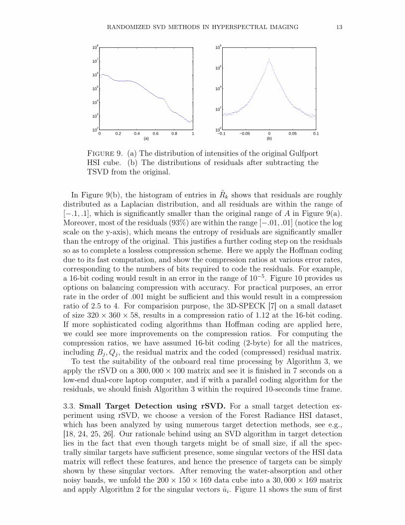
Figure 9. (a) The distribution of intensities of the original GulfportHSI cube. (b) The distributions of residuals after subtracting theTSVD from the original.

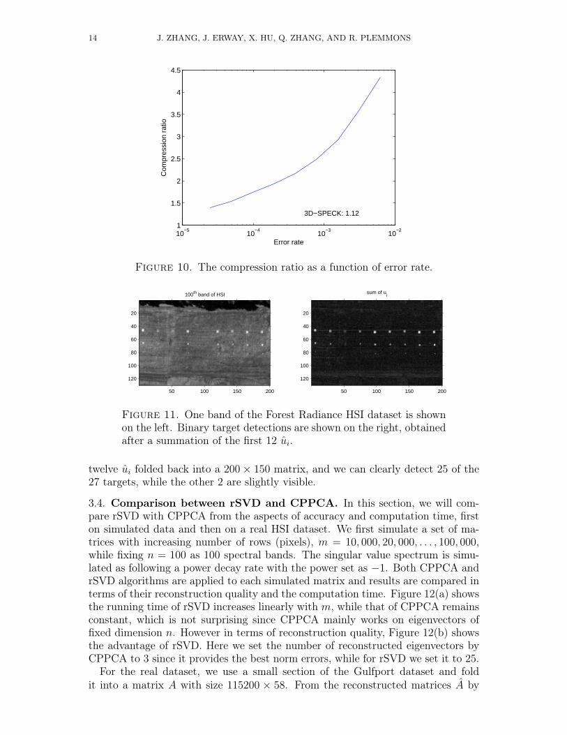
In Figure 9(b), the histogram of entries in Rk shows that residuals are roughlydistributed as a Laplacian distribution, and all residuals are within the range of[−.1, .1], which is significantly smaller than the original range of A in Figure 9(a).Moreover, most of the residuals (93%) are within the range [−.01, .01] (notice the logscale on the y-axis), which means the entropy of residuals are significantly smallerthan the entropy of the original. This justifies a further coding step on the residualsso as to complete a lossless compression scheme. Here we apply the Hoffman codingdue to its fast computation, and show the compression ratios at various error rates,corresponding to the numbers of bits required to code the residuals. For example,a 16-bit coding would result in an error in the range of 10−5. Figure 10 provides usoptions on balancing compression with accuracy. For practical purposes, an errorrate in the order of .001 might be sufficient and this would result in a compressionratio of 2.5 to 4. For comparision purpose, the 3D-SPECK [7] on a small datasetof size 320 × 360 × 58, results in a compression ratio of 1.12 at the 16-bit coding.If more sophisticated coding algorithms than Hoffman coding are applied here,we could see more improvements on the compression ratios. For computing thecompression ratios, we have assumed 16-bit coding (2-byte) for all the matrices,including Bj, Qj, the residual matrix and the coded (compressed) residual matrix.

To test the suitability of the onboard real time processing by Algorithm 3, weapply the rSVD on a 300, 000× 100 matrix and see it is finished in 7 seconds on alow-end dual-core laptop computer, and if with a parallel coding algorithm for theresiduals, we should finish Algorithm 3 within the required 10-seconds time frame.

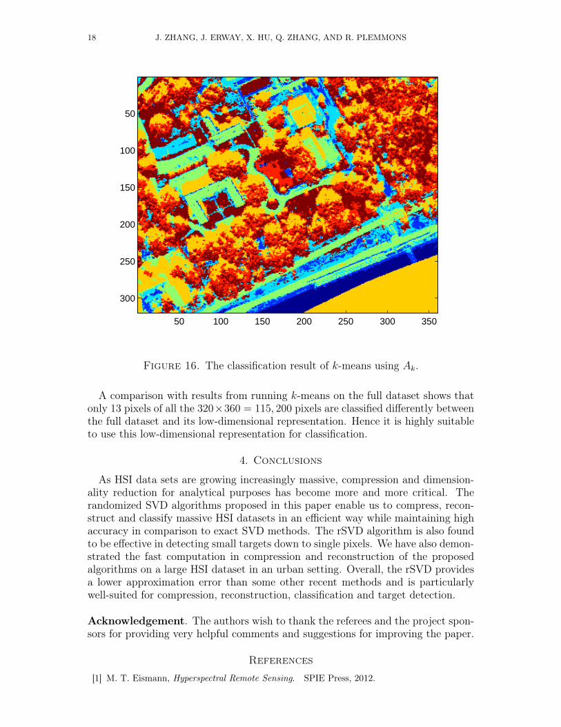
3.3. Small Target Detection using rSVD. For a small target detection ex-periment using rSVD, we choose a version of the Forest Radiance HSI dataset,which has been analyzed by using numerous target detection methods, see e.g.,[18, 24, 25, 26]. Our rationale behind using an SVD algorithm in target detectionlies in the fact that even though targets might be of small size, if all the spec-trally similar targets have sufficient presence, some singular vectors of the HSI datamatrix will reflect these features, and hence the presence of targets can be simplyshown by these singular vectors. After removing the water-absorption and othernoisy bands, we unfold the 200× 150× 169 data cube into a 30, 000× 169 matrixand apply Algorithm 2 for the singular vectors ui. Figure 11 shows the sum of first

14 J. ZHANG, J. ERWAY, X. HU, Q. ZHANG, AND R. PLEMMONS

10−5

10−4

10−3

10−2

1

1.5

2

2.5

3

3.5

4

4.5

Error rate

Com

pres

sion

rat

io

3D−SPECK: 1.12

Figure 10. The compression ratio as a function of error rate.

100th band of HSI

50 100 150 200

20

40

60

80

100

120

sum of ui

50 100 150 200

20

40

60

80

100

120

Figure 11. One band of the Forest Radiance HSI dataset is shownon the left. Binary target detections are shown on the right, obtainedafter a summation of the first 12 ui.

twelve ui folded back into a 200× 150 matrix, and we can clearly detect 25 of the27 targets, while the other 2 are slightly visible.

3.4. Comparison between rSVD and CPPCA. In this section, we will com-pare rSVD with CPPCA from the aspects of accuracy and computation time, firston simulated data and then on a real HSI dataset. We first simulate a set of ma-trices with increasing number of rows (pixels), m = 10, 000, 20, 000, . . . , 100, 000,while fixing n = 100 as 100 spectral bands. The singular value spectrum is simu-lated as following a power decay rate with the power set as −1. Both CPPCA andrSVD algorithms are applied to each simulated matrix and results are compared interms of their reconstruction quality and the computation time. Figure 12(a) showsthe running time of rSVD increases linearly with m, while that of CPPCA remainsconstant, which is not surprising since CPPCA mainly works on eigenvectors offixed dimension n. However in terms of reconstruction quality, Figure 12(b) showsthe advantage of rSVD. Here we set the number of reconstructed eigenvectors byCPPCA to 3 since it provides the best norm errors, while for rSVD we set it to 25.

For the real dataset, we use a small section of the Gulfport dataset and foldit into a matrix A with size 115200 × 58. From the reconstructed matrices A by

RANDOMIZED SVD METHODS IN HYPERSPECTRAL IMAGING 15

0 2 4 6 8 10

x 104

0

0.2

0.4

0.6

0.8

1

1.2

1.4

n

seco

nds

(a)

0 2 4 6 8 10

x 104

0

0.05

0.1

0.15

0.2

0.25

0.3

0.35

0.4

0.45

0.5

n

norm

err

or

(b)

rSVDCPPCA

rSVDCPPCA

Figure 12. (a) Running times of rSVD and CPPCA. (b) Recon-struction qualities of rSVD and CPPCA.

0.2 0.25 0.3 0.35 0.4 0.45 0.510

12

14

16

18

20

22

24

26

28

30

relative subspace dimension, k/n

aver

age

SN

R (

dB)

CPPCArSVDrSVD (q=2)

Figure 13. Comparison of reconstruction qualities of rSVD and CP-PCA in terms of SNR.

both methods, with varying rank k we compare their reconstruction qualities interms of signal-to-noise ratio (SNR) in Figure 13, and the computation time inTable 1. Again we observe the better reconstruction quality though slightly slowercomputation of rSVD when compared to CPPCA.

Table 1. Computation times (seconds) of rSVD and CPPCA.

k/n 0.1 0.15 0.2 0.3 0.4 0.5

rSVD 0.212 0.292 0.390 0.707 0.897 1.264

CPPCA 0.247 0.305 0.331 0.368 0.399 0.509

Next, we compare the accuracy of the reconstruction of the eigenvectors, vi, ofthe covariance matrix of A by these two methods. Given that PCA is an extremelyuseful tool in HSI data analysis, e.g., for classification and target detection, it is

16 J. ZHANG, J. ERWAY, X. HU, Q. ZHANG, AND R. PLEMMONS

Figure 14. Comparison of reconstructed egenvectors by rSVD andCPPCA with the true ones.

essential to obtain a quality reconstruction of the eigenvectors vi by rSVD in termsof accuracy and efficiency. Here we simulate a 10, 000× 100 matrix A with orthog-onalized random matrices, Uo and Vo, and a power-decay singular value spectrumin Σo, with he power set as −1. Then we run both algorithms for 1, 000 times and,within each time, we compute the angles between eigenvectors by CPPCA and thetrue ones, and between eigenvectors by rSVD and the true ones. The first rowof Figure 14 shows the histograms of angles between the first eight reconstructedeigenvectors by CPPCA and the true ones, while the second row shows the his-tograms of the angles between the first eight eigenvectors by rSVD and the trueones. We can see that the first three or four eigenvectors by CPPCA appear to beclose to the true ones, while the rest are not. Hence if using more than four eigen-vectors reconstructed by CPPCA, we observe a decrease in reconstruction qualityor an increase in the norm error. However in the second row, we see good accuracyof the eigenvectors computed by rSVD.

3.5. Classification of HSI Data by rSVD. Since the projection of a HSI datamatrix by its truncated singular matrix, i.e.,

AP = AVk, (13)

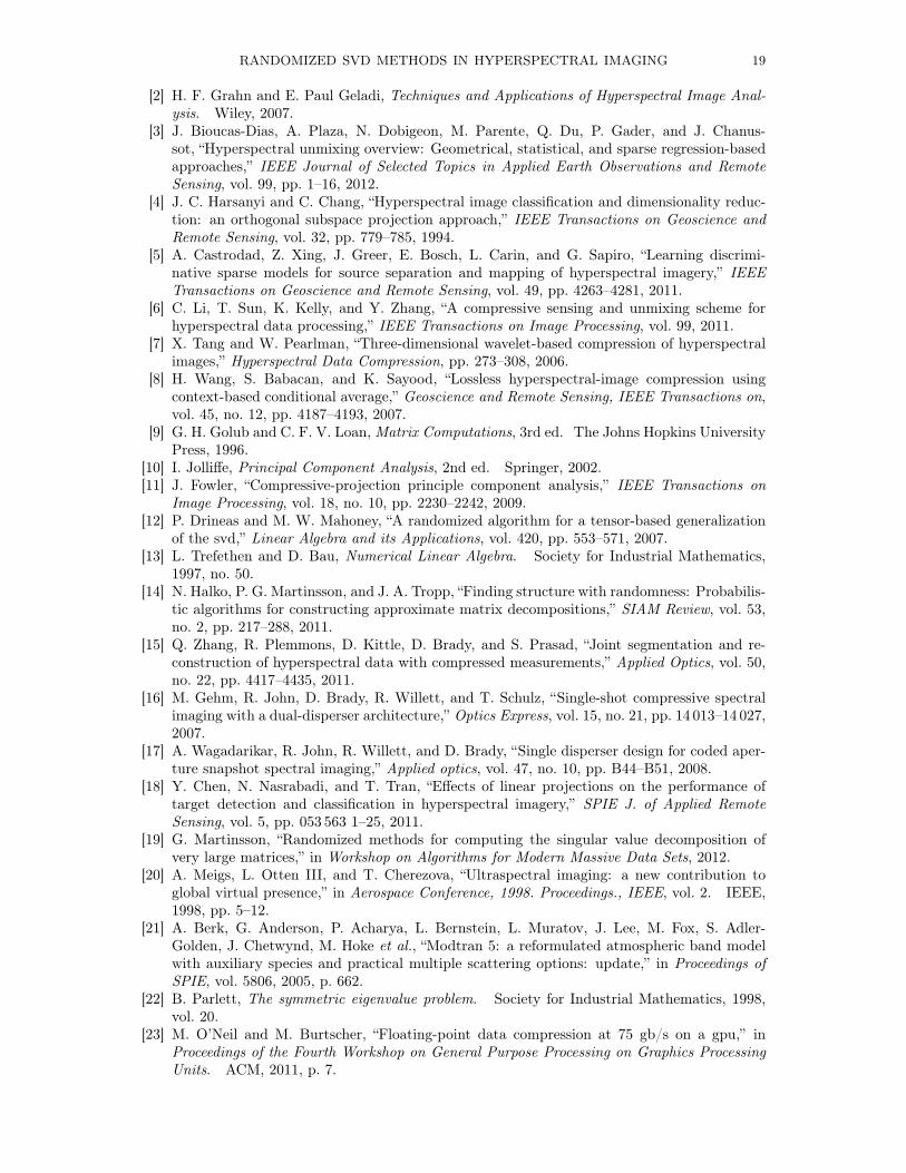
contains most of the information in the original matrix A, we can use any clas-sification algorithm, such as the popular k-means, to classify HSI data, but alsouse its representation in a lower dimensional space. Consider a small section ofthe Gulfport dataset. Figure 15 shows the first 8 columns of AP . From the firstsub-figure, we see that most information of the hyperspectral image is containedin the first column, while the second column almost contains the rest of the infor-mation which the first column does not contain. The rest of the columns containinformation at more detailed and spatially clustered levels. Figure 16 shows theresult of classification by k-means, where we can see the low-reflectance water andshadows in yellow, the foliage in red, the grass in dark red, the pavement in green,

RANDOMIZED SVD METHODS IN HYPERSPECTRAL IMAGING 17

100 200 300

100

200

300

100 200 300

100

200

300

100 200 300

100

200

300

100 200 300

100

200

300

100 200 300

100

200

300

100 200 300

100

200

300

100 200 300

100

200

300

100 200 300

100

200

300

Figure 15. Plots of the first 8 columns of AP .

and high-reflectance beach sand in dark blue, and dirt/sandy grass in blue and lightblue.

18 J. ZHANG, J. ERWAY, X. HU, Q. ZHANG, AND R. PLEMMONS

50 100 150 200 250 300 350

50

100

150

200

250

300

Figure 16. The classification result of k-means using Ak.

A comparison with results from running k-means on the full dataset shows thatonly 13 pixels of all the 320×360 = 115, 200 pixels are classified differently betweenthe full dataset and its low-dimensional representation. Hence it is highly suitableto use this low-dimensional representation for classification.

4. Conclusions

As HSI data sets are growing increasingly massive, compression and dimension-ality reduction for analytical purposes has become more and more critical. Therandomized SVD algorithms proposed in this paper enable us to compress, recon-struct and classify massive HSI datasets in an efficient way while maintaining highaccuracy in comparison to exact SVD methods. The rSVD algorithm is also foundto be effective in detecting small targets down to single pixels. We have also demon-strated the fast computation in compression and reconstruction of the proposedalgorithms on a large HSI dataset in an urban setting. Overall, the rSVD providesa lower approximation error than some other recent methods and is particularlywell-suited for compression, reconstruction, classification and target detection.

Acknowledgement. The authors wish to thank the referees and the project spon-sors for providing very helpful comments and suggestions for improving the paper.

References

[1] M. T. Eismann, Hyperspectral Remote Sensing. SPIE Press, 2012.

RANDOMIZED SVD METHODS IN HYPERSPECTRAL IMAGING 19

[2] H. F. Grahn and E. Paul Geladi, Techniques and Applications of Hyperspectral Image Anal-ysis. Wiley, 2007.

[3] J. Bioucas-Dias, A. Plaza, N. Dobigeon, M. Parente, Q. Du, P. Gader, and J. Chanus-sot, “Hyperspectral unmixing overview: Geometrical, statistical, and sparse regression-basedapproaches,” IEEE Journal of Selected Topics in Applied Earth Observations and RemoteSensing, vol. 99, pp. 1–16, 2012.

[4] J. C. Harsanyi and C. Chang, “Hyperspectral image classification and dimensionality reduc-tion: an orthogonal subspace projection approach,” IEEE Transactions on Geoscience andRemote Sensing, vol. 32, pp. 779–785, 1994.

[5] A. Castrodad, Z. Xing, J. Greer, E. Bosch, L. Carin, and G. Sapiro, “Learning discrimi-native sparse models for source separation and mapping of hyperspectral imagery,” IEEETransactions on Geoscience and Remote Sensing, vol. 49, pp. 4263–4281, 2011.

[6] C. Li, T. Sun, K. Kelly, and Y. Zhang, “A compressive sensing and unmixing scheme forhyperspectral data processing,” IEEE Transactions on Image Processing, vol. 99, 2011.

[7] X. Tang and W. Pearlman, “Three-dimensional wavelet-based compression of hyperspectralimages,” Hyperspectral Data Compression, pp. 273–308, 2006.

[8] H. Wang, S. Babacan, and K. Sayood, “Lossless hyperspectral-image compression usingcontext-based conditional average,” Geoscience and Remote Sensing, IEEE Transactions on,vol. 45, no. 12, pp. 4187–4193, 2007.

[9] G. H. Golub and C. F. V. Loan, Matrix Computations, 3rd ed. The Johns Hopkins UniversityPress, 1996.

[10] I. Jolliffe, Principal Component Analysis, 2nd ed. Springer, 2002.[11] J. Fowler, “Compressive-projection principle component analysis,” IEEE Transactions on

Image Processing, vol. 18, no. 10, pp. 2230–2242, 2009.[12] P. Drineas and M. W. Mahoney, “A randomized algorithm for a tensor-based generalization

of the svd,” Linear Algebra and its Applications, vol. 420, pp. 553–571, 2007.[13] L. Trefethen and D. Bau, Numerical Linear Algebra. Society for Industrial Mathematics,

1997, no. 50.[14] N. Halko, P. G. Martinsson, and J. A. Tropp, “Finding structure with randomness: Probabilis-

tic algorithms for constructing approximate matrix decompositions,” SIAM Review, vol. 53,no. 2, pp. 217–288, 2011.

[15] Q. Zhang, R. Plemmons, D. Kittle, D. Brady, and S. Prasad, “Joint segmentation and re-construction of hyperspectral data with compressed measurements,” Applied Optics, vol. 50,no. 22, pp. 4417–4435, 2011.

[16] M. Gehm, R. John, D. Brady, R. Willett, and T. Schulz, “Single-shot compressive spectralimaging with a dual-disperser architecture,” Optics Express, vol. 15, no. 21, pp. 14 013–14 027,2007.

[17] A. Wagadarikar, R. John, R. Willett, and D. Brady, “Single disperser design for coded aper-ture snapshot spectral imaging,” Applied optics, vol. 47, no. 10, pp. B44–B51, 2008.

[18] Y. Chen, N. Nasrabadi, and T. Tran, “Effects of linear projections on the performance oftarget detection and classification in hyperspectral imagery,” SPIE J. of Applied RemoteSensing, vol. 5, pp. 053 563 1–25, 2011.

[19] G. Martinsson, “Randomized methods for computing the singular value decomposition ofvery large matrices,” in Workshop on Algorithms for Modern Massive Data Sets, 2012.

[20] A. Meigs, L. Otten III, and T. Cherezova, “Ultraspectral imaging: a new contribution toglobal virtual presence,” in Aerospace Conference, 1998. Proceedings., IEEE, vol. 2. IEEE,1998, pp. 5–12.

[21] A. Berk, G. Anderson, P. Acharya, L. Bernstein, L. Muratov, J. Lee, M. Fox, S. Adler-Golden, J. Chetwynd, M. Hoke et al., “Modtran 5: a reformulated atmospheric band modelwith auxiliary species and practical multiple scattering options: update,” in Proceedings ofSPIE, vol. 5806, 2005, p. 662.

[22] B. Parlett, The symmetric eigenvalue problem. Society for Industrial Mathematics, 1998,vol. 20.

[23] M. O’Neil and M. Burtscher, “Floating-point data compression at 75 gb/s on a gpu,” inProceedings of the Fourth Workshop on General Purpose Processing on Graphics ProcessingUnits. ACM, 2011, p. 7.

20 J. ZHANG, J. ERWAY, X. HU, Q. ZHANG, AND R. PLEMMONS

[24] R. Olsen, S. Bergman, and R. Resmini, “Target detection in a forest environment usingspectral imagery,” in Imaging Spectrometry III, Proceedings of the SPIE, vol. 3118, 1997, pp.46–56.

[25] C. Chang, “Target signature-constrained mixed pixel classification for hyperspectral imagery,”Geoscience and Remote Sensing, IEEE Transactions on, vol. 40, no. 5, pp. 1065–1081, 2002.

[26] B. Thai and G. Healey, “Invariant subpixel material detection in hyperspectral imagery,”Geoscience and Remote Sensing, IEEE Transactions on, vol. 40, no. 3, pp. 599–608, 2002.

J. Jiang, Department of Mathematics, Wake Forest University, Winston-Salem,NC 27109

E-mail address: zhang210@wfu.edu

J. Erway, Department of Mathematics, Wake Forest University, Winston-Salem,NC 27109

E-mail address: erwayjb@wfu.edu

X. Hu, Department of Mathematics, Wake Forest University, Winston-Salem,NC 27109

E-mail address: hux@wfu.edu

Q. Zhang, Department of Biostatistical Sciences, Wake Forest School of Medicine,Winston-Salem, NC 27157

E-mail address: qizhang@wakehealth.edu

R. Plemmons, Corresponding Author, Departments of Mathematics and Com-puter Science, Wake Forest University, Winston-Salem, NC 27109

E-mail address: plemmons@wfu.edu, web page: http://www.wfu.edu/˜plemmons