Randomized Benchmarking with Confidence

Joel J. Wallman1, 2 and Steven T. Flammia2

1Institute for Quantum Computing, University of Waterloo, Waterloo, Canada2Centre for Engineered Quantum Systems, School of Physics,

The University of Sydney, Sydney, NSW 2006, Australia

(Dated: December 18, 2015)

Randomized benchmarking is a promising tool for characterizing the noise in experimentalimplementations of quantum systems. In this paper, we prove that the estimates producedby randomized benchmarking (both standard and interleaved) for arbitrary Markovian noisesources are remarkably precise by showing that the variance due to sampling random gatesequences is small. We discuss how to choose experimental parameters, in particular thenumber and lengths of random sequences, in order to characterize average gate errors withrigorous confidence bounds. We also show that randomized benchmarking can be used to reli-ably characterize time-dependent Markovian noise (e.g., when noise is due to a magnetic fieldwith fluctuating strength). Moreover, we identify a necessary property for time-dependentnoise that is violated by some sources of non-Markovian noise, which provides a test fornon-Markovianity.

I. INTRODUCTION

One of the key obstacles to realizing large-scale quantum computation is the need for errorcorrection and fault tolerance [1], which require the coherent implementation of unitary operationsto high precision. Characterizing the accuracy of an experimental implementation of a unitaryoperation is therefore an important prerequisite for constructing a large-scale quantum computer.

It is possible to completely characterize an experimental implementation of a unitary using fullquantum process tomography [2, 3]. However, this approach has several major deficiencies whenapplied to large quantum systems. Firstly, it is provably exponential in the number of qubits of thesystem for any procedure that can identify general noise sources and hence it cannot be performedpractically for even intermediate numbers of qubits, despite improvements such as compressedsensing [4, 5]. Secondly, it is sensitive to state preparation and measurement (SPAM) errors, whichcreate a noise floor below which an accurate process estimation becomes impossible [6]. Finally,it does not capture any notion of systematic, time-dependent errors that can arise from applyingmany unitaries in sequence.

One can avoid the exponential scaling by accepting a partial characterization of an experimen-tal implementation. A partial characterization of, for example, the average error rate and/or theworst-case error rate compared to a perfect implementation of a target unitary is typically enoughto determine whether an experimental implementation of a unitary is sufficient for achieving fault-tolerance in a specific scheme for fault-tolerant quantum computation. Such partial characteri-zations can be obtained efficiently (in the number of quantum systems) using either randomizedbenchmarking [7–12] or direct fidelity estimation [13, 14].

While direct fidelity estimation gives an unconditional and assumption-free estimate of the av-erage gate fidelity, it is prone to state preparation and measurement (SPAM) errors, which leadsto conflation of noise sources. Thus, a key advantage of randomized benchmarking is that it isnot sensitive to SPAM errors. Unfortunately, however, current proposals for randomized bench-marking assume that the noise is time-independent, although time-dependence can be partiallycharacterized by a deviation from the expected fidelity decay curve [9, 10]. Furthermore, exper-imental implementations of randomized benchmarking typically use on the order of 100 randomsequences of Clifford gates, which is three orders of magnitude smaller than the number of se-

arX

iv:1

404.

6025

v4 [

quan

t-ph

] 1

7 D

ec 2

015

2

quences suggested by the rigorous bounds in Ref. [10] to obtain an accuracy comparable to theclaimed experimental accuracies [12, 15]. Numerical investigations of a variety of noise modelshave shown that between 10–100 random sequences for each length are sufficient to provide a tightestimate of the average gate fidelity [16]. Ideally, one would like to combine the advantages of bothrandomized benchmarking and direct fidelity estimation to achieve a method that is insensitive toSPAM, requires few measurements, is nearly assumption-free (i.e., does not assume a specific noisemodel), and comes with rigorous guarantees on the errors involved.

In this paper, we provide a new analysis of randomized benchmarking which brings it closer inline with this ideal. We first show that the standard protocol can be modified to provide a meansof estimating the time-dependent average gate fidelity (which characterizes the average error rate),provided that the gate-dependent fluctuations at each time step are sufficiently small. Under theassumption that the noise is Markovian (that is, that the noise can be written as a sequence of noisychannels acting on the system of interest), all the time-dependent parameters that are estimatedby our procedure are upper-bounded by 1, so if some of the parameters are observed to be greaterthan 1, the experimental noise must be non-Markovian.

We then provide a rigorous justification for taking a small number of random sequences at eachlength that is on the same order as used in practice by obtaining bounds on the variance due tosampling gate sequences. Our work complements the approach of Ref. [16], where it was shown thatthe width of the confidence interval for the parameters extracted from randomized benchmarkingis on the order of the square root of the variance. Our work therefore proves that this confidenceinterval is generally very narrow, that is, the parameters extracted from randomized benchmarkingare determined with high precision.

Numerically, we observe that our bounds (at least for qubits) are saturated and so cannot beimproved without further assumptions on the noise (e.g., that the noise is diagonal in the Paulibasis). Therefore any experiments using fewer random sequences than justified by our analysis(unless there is solid evidence that the noise has a specific structure) will potentially underestimatethe error due to sampling random sequences.

As a particular example, our results provide a rigorous proof that for single-qubit noise with anaverage error rate of 10−4, the error for randomized benchmarking with 100 random sequences of100 random gates will be less than 0.9% with 99% confidence. If we use the parameters estimatedin the experiment of Ref. [15], with 100 random sequences of length 987 at an average error rateof 2× 10−5, we find the error is less than .8% with 99% confidence.

We emphasize that our results are solely in terms of the number of random gate sequences, anda given sequence must still be repeated many times to gather statistics about expectation valuesof an observable. This is of course an unavoidable consequence of quantum mechanics. However,these statistical fluctuations in the estimates of expectation values can be analyzed separately withstandard statistical tools for binomial distributions or with the recent Bayesian methods introducedin [17] and combined seamlessly with our results.

In order to give a rigorous statement of results, we will first review the randomized benchmarkingprotocol.

II. THE RANDOMIZED BENCHMARKING PROTOCOL

The goal of randomized benchmarking is to efficiently but partially characterize the average noisein an experimental implementation of a group G = {g1, . . . , g|G|} ⊂ U(d) of operations acting on ad-dimensional quantum system. In order to characterize the average noise in an implementation ofG using randomized benchmarking, we require G to be a unitary 2-design (e.g., the Clifford groupon n qubits for d = 2n), meaning that sampling over G reproduces the second moments of the Haar

3

measure [18, 19]. To accomplish this, the following protocol is implemented.

• Choose a random sequence s = s1 . . . sm ∈ Nm|G| of m integers chosen uniformly at random

from N|G| = {1, . . . , |G|}.

• Prepare a d-dimensional system in some state ρ (usually taken to be the pure state |0〉).

• At each time step t = 0, . . . ,m, apply gt where gt = gst and g0 :=∏mt=1 g

−1t . Alternatively,

to perform interleaved randomized benchmarking for the gate gint ∈ G, apply gt,int wheregt,int = gintgt for t 6= 0 and, as before, g0,int =

∏mt=1 g

−1t,int. (In general, each gate must be

compiled into a sequence of elementary gates as well.)

• Perform a POVM {E,1− E} for some E (usually taken to be |0〉〈0|) and repeat with thesequence s sufficiently many times to obtain an estimate of the probability Fm,s = p(E|s, ρ)to a suitable precision.

We can regard the probability Fm,s as a realization of a random variable Fm. We will denotethe variance of the distribution {Fm,s : s ∈ N|G|} for a fixed m by σ2m. Averaging Fm,s over a

number of random sequences will give an estimate Fm of Fm, the average of Fm,s over all sequencess of fixed length m (that is, Fm is the expectation of the random variable Fm). The accuracy ofthis estimate will be a function of the number of random sequences and σ2m.

Obtaining estimates Fm for multiple m and fitting to the model

Fm = A+Bfm (1)

will give an estimate of f provided that the noise does not depend too strongly on the targetgate [10], where [20]

f =dFavg(E)− 1

d− 1(2)

and

Favg(E) =

∫dψTr

[ψE(ψ)

](3)

is the average gate fidelity of a noise channel E with respect to the identity channel and dψ isthe uniform Haar measure over all pure states. The average gate fidelity of E gives the averageprobability that preparing a state ψ, applying E and then measuring {ψ,1 − ψ} will give theoutcome ψ, averaged over all pure states ψ.

For standard randomized benchmarking, E is the error channel per operation, averaged overall operations in G. For interleaved benchmarking, E is the error channel on a composite channel,namely, the interleaved channel composed with an element of G, averaged over all G. We note inpassing that separating the error in the interleaved channel from the error in the composite channelis one of the key difficulties in obtaining meaningful results from interleaved benchmarking [21],though we do not address this issue here.

III. STATEMENT OF RESULTS AND PAPER OUTLINE

The first principal contribution of this paper is to show that the number of random sequencesthat need to be averaged is comparable to the number actually used in contemporary experiments(compared to previous best estimates, which require 3 orders of magnitude more random sequences

4

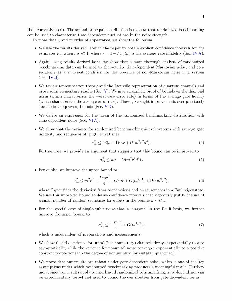
than currently used). The second principal contribution is to show that randomized benchmarkingcan be used to characterize time-dependent fluctuations in the noise strength.

In more detail, and in order of appearance, we show the following.

• We use the results derived later in the paper to obtain explicit confidence intervals for theestimates Fm when mr � 1, where r = 1−Favg(E) is the average gate infidelity (Sec. IV A).

• Again, using results derived later, we show that a more thorough analysis of randomizedbenchmarking data can be used to characterize time-dependent Markovian noise, and con-sequently as a sufficient condition for the presence of non-Markovian noise in a system(Sec. IV B).

• We review representation theory and the Liouville representation of quantum channels andprove some elementary results (Sec. V). We give an explicit proof of bounds on the diamondnorm (which characterizes the worst-case error rate) in terms of the average gate fidelity(which characterizes the average error rate). These give slight improvements over previouslystated (but unproven) bounds (Sec. V D).

• We derive an expression for the mean of the randomized benchmarking distribution withtime-dependent noise (Sec. VI A).

• We show that the variance for randomized benchmarking d-level systems with average gateinfidelity and sequences of length m satisfies

σ2m ≤ 4d(d+ 1)mr +O(m2r2d4) . (4)

Furthermore, we provide an argument that suggests that this bound can be improved to

σ2m ≤ mr +O(m2r2d4) . (5)

• For qubits, we improve the upper bound to

σ2m ≤ m2r2 +7mr2

4+ 6δmr +O(m2r3) +O(δm2r2) , (6)

where δ quantifies the deviation from preparations and measurements in a Pauli eigenstate.We use this improved bound to derive confidence intervals that rigorously justify the use ofa small number of random sequences for qubits in the regime mr � 1.

• For the special case of single-qubit noise that is diagonal in the Pauli basis, we furtherimprove the upper bound to

σ2m ≤11mr2

4+O(m2r3) , (7)

which is independent of preparations and measurements.

• We show that the variance for unital (but nonunitary) channels decays exponentially to zeroasymptotically, while the variance for nonunital noise converges exponentially to a positiveconstant proportional to the degree of nonunitality (as suitably quantified).

• We prove that our results are robust under gate-dependent noise, which is one of the keyassumptions under which randomized benchmarking produces a meaningful result. Further-more, since our results apply to interleaved randomized benchmarking, gate dependence canbe experimentally tested and used to bound the contribution from gate-dependent terms.

5

IV. ANALYZING DATA FROM RANDOMIZED BENCHMARKING WITH FINITESAMPLING

In this section, we summarize the implications of our results for analyzing the data obtainedfrom randomized benchmarking experiments. In particular, we derive confidence intervals for theestimates Fm of Fm and show how randomized benchmarking can be used to characterize time-dependent noise.

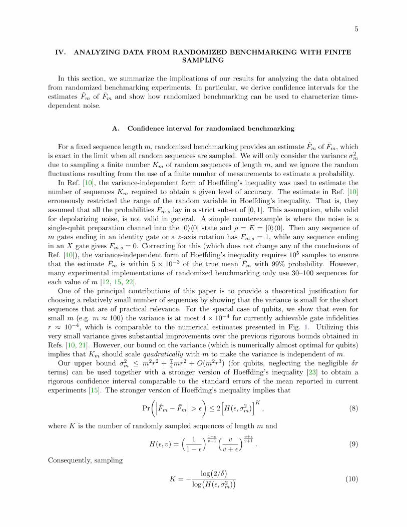
A. Confidence interval for randomized benchmarking

For a fixed sequence length m, randomized benchmarking provides an estimate Fm of Fm, whichis exact in the limit when all random sequences are sampled. We will only consider the variance σ2mdue to sampling a finite number Km of random sequences of length m, and we ignore the randomfluctuations resulting from the use of a finite number of measurements to estimate a probability.

In Ref. [10], the variance-independent form of Hoeffding’s inequality was used to estimate thenumber of sequences Km required to obtain a given level of accuracy. The estimate in Ref. [10]erroneously restricted the range of the random variable in Hoeffding’s inequality. That is, theyassumed that all the probabilities Fm,s lay in a strict subset of [0, 1]. This assumption, while validfor depolarizing noise, is not valid in general. A simple counterexample is where the noise is asingle-qubit preparation channel into the |0〉〈0| state and ρ = E = |0〉〈0|. Then any sequence ofm gates ending in an identity gate or a z-axis rotation has Fm,s = 1, while any sequence endingin an X gate gives Fm,s = 0. Correcting for this (which does not change any of the conclusions ofRef. [10]), the variance-independent form of Hoeffding’s inequality requires 105 samples to ensurethat the estimate Fm is within 5 × 10−3 of the true mean Fm with 99% probability. However,many experimental implementations of randomized benchmarking only use 30–100 sequences foreach value of m [12, 15, 22].

One of the principal contributions of this paper is to provide a theoretical justification forchoosing a relatively small number of sequences by showing that the variance is small for the shortsequences that are of practical relevance. For the special case of qubits, we show that even forsmall m (e.g. m ≈ 100) the variance is at most 4 × 10−4 for currently achievable gate infidelitiesr ≈ 10−4, which is comparable to the numerical estimates presented in Fig. 1. Utilizing thisvery small variance gives substantial improvements over the previous rigorous bounds obtained inRefs. [10, 21]. However, our bound on the variance (which is numerically almost optimal for qubits)implies that Km should scale quadratically with m to make the variance is independent of m.

Our upper bound σ2m ≤ m2r2 + 74mr

2 + O(m2r3) (for qubits, neglecting the negligible δrterms) can be used together with a stronger version of Hoeffding’s inequality [23] to obtain arigorous confidence interval comparable to the standard errors of the mean reported in currentexperiments [15]. The stronger version of Hoeffding’s inequality implies that

Pr

(∣∣∣Fm − Fm∣∣∣ > ε

)≤ 2[H(ε, σ2m)

]K, (8)

where K is the number of randomly sampled sequences of length m and

H(ε, v) =( 1

1− ε) 1−εv+1( v

v + ε

) v+εv+1

. (9)

Consequently, sampling

K = − log(2/δ)

log(H(ε, σ2m)

) (10)

6

random sequences is sufficient to obtain an absolute precision of ε with probability 1− δ. Since ris determined by the fitting procedure, which in turn depends on the uncertainties, this procedurewould be applied recursively with an initial upper bound on r. Similarly, for qudits, a straightfor-ward generalization of the above argument can be used, but with σ2m ≤ 4d(d+ 1)mr+O(d4m2r2).(There are various inefficiencies in this estimate which mean that it does not reduce to the sameanswer as above for d = 2; see Theorem 10 for more details.)

To get a feel for the sort of estimates that this bound provides, consider the following parametersfor a single-qubit benchmarking experiment: m = 100, r = 10−4, ε = 1%, δ = 1%, and use ourupper bound of σ2m = m2r2 + 7

4mr2 (ignoring the higher-order terms). Then our bound shows

that K = 145 random sequences suffices. This is an improvement by orders of magnitude over theprevious best rigorously justifiable upper bound of 105 using the variance-independent Hoeffdinginequality [10].

Importantly, however, we note that the quadratic scaling with m in the regime mr � 1 seems tobe necessary (see Fig. 1). Even in the optimal case of noise that is diagonal in the Pauli basis, Km

would still need to scale linearly with m to make the variance independent of m (where having thevariance depend on m would generally cause less weight to be assigned to larger m when fitting).The linear scaling can be understood intuitively as following from the fact that there are m placesfor an error in a sequence of length m, and the errors could add up in the worst case. Therefore,a corollary of our result is that longer sequence lengths should be averaged over more randomsequences in this regime.

Furthermore, we prove in Sec. VII that there are noise sources such that the variance dueto sampling random sequences is constant (or decays on an arbitrarily long timescale). If suchnoise sources (including nonunital noise and any unitary noise, such as over- and under-rotations)are believed to be present, substantially more random sequences need to be sampled. As such,randomized benchmarking is most reliable in the regime mr � 1, although, since the next lowestorder terms in our bound are δm2r2 and m2r3, the lowest order bounds on the variance should beapproximately valid for mr ≈ 0.1.

B. Characterizing time-dependent noise

The original presentation of randomized benchmarking assumed that the noise was approxi-mately time independent (i.e., independent of the time step at which the gate is applied), with anyMarkovian time-dependence being partially characterized by deviations from the time-independentcase [10]. However, in many practical applications there may be a nonnegligible time dependence,which it would be desirable to characterize more fully.

We show that randomized benchmarking can also be used to characterize time-dependent noise,provided the gate-dependence is negligible (in the sense established in Theorem 18) and that thetime-dependent noise is identically distributed between different experiments. However, the numberof random sequences of length m will typically need to be increased relative to the number requiredfor time-independent noise. In particular, we will show in Theorem 8 that

Fm = A+Bm∏t=1

ft , (11)

where A and B are constants that depend only upon the preparation and measurement procedures(and so account for SPAM) and the average gate fidelity at time t is Ft = ft + (1− ft)/d, where dis the dimensionality of the system being benchmarked. In the case of time-independent noise, ftis a constant and Eq. (11) reduces to the standard equation for the fidelity decay curve.

7

0 20 40 60 80 100

0

1

2

3

4

5

6

7·10−4

Sequence length m

Var

ian

ceσ2 m

FIG. 1. Plot of a random sampling of the exact variance σ2m as a function of the sequence length m for

randomized benchmarking with 100 randomly generated, time-independent noisy qubit channels. The noisewas sampled from the set of extremal qubit channels, characterized in Ref. [24], with average gate infidelityr . 2.69 × 10−4. Each channel was evolved for increasing sequence lengths to track the behavior of thevariance as a function of m, which is why the data points track parabolic curves (furthermore, the spreadin the parabolic curves is generated by the spread in the infidelity of the samples). The green curve is the

upper bound σ2m = m2r2 + 7mr2

4 , where we neglect the corrections to the bound at order O(m2r3) andcorrections due to measurement imprecision. Note that our bound is almost optimal. Our analytic resultsshow that the variance σ2

m will increase with m, at least until some threshold sequence length where theexponential decay for generic channels proven in Theorem 17 begins to dominate.

By performing randomized benchmarking for a set of sequence lengths m1 and m2, we canestimate Fmj with associated uncertainties δj . Combining these estimates with a procedure for

obtaining an estimate A of A with associated uncertainty δA [25], we can estimate the ratio

Fm2 − AFm1 − A

=

m2∏t=m1+1

ft (12)

with uncertainty on the order of

δ1,2,A ≈√

(δ1 + δA)2 + (δ2 + δA)2 . (13)

Therefore we can estimate the average gate infidelity r over the time interval [m1 + 1,m2].From our rigorous analysis, we can infer that δ1 and δ2 will be small for small mjr, while δA willbe determined only by finite measurement statistics. Furthermore, when m2 ≈ m1,

∏m2t=m1+1 ft ≈

1−r(m2−m1) and so the above method gives a reliable method of characterizing the time-dependentgate fidelity.

8

We also note that if there are no temporal correlations in the noise, than all of the parametersrt (where rt is the average gate infidelity at time r) are lower-bounded by zero. Therefore anynegative values (or average values) of rt are an indicator of temporal correlations in the noise, thatis, of non-Markovian behavior.

V. MATHEMATICAL PRELIMINARIES

Randomized benchmarking involves composing random sequences of quantum channels that aresampled in a way which approximates a group average. For this reason, it is natural to considerboth the representation theory of groups and the structure of quantum channels, especially thecomposition of channels. In this section we collect several mathematical results in this vein thatwe will need to prove our main results. We begin by considering group representation theory, andin particular prove a proposition showing how the tensor product of certain representations coupletogether. Most of this material is standard and can be found in any textbook on the subject,e.g. [26].

A. Representation Theory and Some Useful Lemmas

A representation (rep) of a group G is a pair (φ, V ), where V is vector space known as therepresentation space (which we always take to be Rd or Cd for different values of d) and φ : G →GL(V )—where GL(V ) is the general linear group over V—is a homomorphism. A rep is faithful ifφ is injective and unitary (resp. orthogonal) if φ(g) is a unitary (resp. orthogonal) operator forall g ∈ G. The dimension of a rep is the dimension of V . A subrepresentation (subrep) is a pair(φW ,W ) such that φ(g)W ⊆ W for all g ∈ G and φW denotes the restriction of φ to the subspaceW . We sometimes refer to a space, subspace, or homomorphism as being a rep or subrep, with thecomplementary ingredients understood from the context.

A rep is called irreducible or an irrep if the only subreps are ∅ and V . Since the reps we considerare unitary reps of compact groups, if W is a subrep of V then the orthogonal complement W⊥

is a subrep as well. Therefore any rep can be decomposed into a direct sum of irreps, which mayoccur with some multiplicity. Any basis that decomposes a rep into a direct sum of irreps is calleda Schur basis.

The simplest rep is the trivial rep (1,C), which is also an irrep. The trivial rep is defined forany group G and take any element of G to 1. While the trivial rep deserves its name, it frequentlyappears as a subrep of tensor powers of other reps and so will appear throughout this paper.

The randomized benchmarking protocol is designed so that the sequence of operators appliedto a system correspond to noise channels conjugated by uniformly random elements of a groupG. Given a rep (φ, V ) of a group G, a matrix A ∈ GL(V ) and an element g ∈ G, we defineAg = φ(g)Aφ(g−1). The uniform average of this action on A is called the G-twirl of A, and is givenby AG = |G|−1∑g∈G A

g.

Note that, for notational convenience, the map φ is left implicit but will always be obvious giventhe dimensionality of the matrix being twirled. An important property of AG is that it commuteswith the action of G for any rep (φ, V ) (reducible or not) since φ is a homomorphism and G is agroup. That is, AG = (Ag)G = (AG)g for all g ∈ G.

Expressions for the expected value Fm and variance σ2m for the randomized benchmarkingprotocol for a fixed value of m will be obtained using the following propositions.

Proposition 1. Let (φ,Cd) be a nontrivial d-dimensional irreducible representation of a group Gand A ∈ GL(Cd), B ∈ GL(Cd+1). Then

9

• AG = a1d;

• BG = B11 ⊕ b1d [where the representation of G is (1⊕ φ,Cd+1)]; and

• ∑g∈G φ(g) = 0,

where a = TrA/d and b = (TrB −B11)/d.

Proof. All three statements follow directly from Schur’s Lemma [26]. �

Proposition 2. If (φ, V ) is an irreducible representation of a finite group G with a real-valuedcharacter χφ, then the trivial representation is a subrepresentation of (φ, V )⊗2 with multiplicity 1.

Proof. As the rep is irreducible, Schur’s orthogonality relations [26] give

|G| =∑g∈G

χφ(g)∗χφ(g) =∑g∈G

χφ(g)2 =∑g∈G

χφ⊗2(g)χ1(g) , (14)

where we have used χφ⊗2(g) = [χφ(g)]2 and that the character for the trivial representation isχ1(g) = 1 for all g ∈ G. �

B. The Liouville Representation of Quantum Channels

A quantum channel is a linear map E : Dd1 → Dd2 , where Dd is the set of d-dimensional densityoperators. Quantum channels can be represented in a variety of equivalent ways, with differentrepresentations naturally suited to particular applications.

In this paper, we will primarily use the Liouville representation because it is defined so thatquantum channels compose under matrix multiplication. We occasionally also use the Choi repre-sentation in order to apply results from the literature, but we will introduce it only as required.

1. States and measurements

We begin by introducing the Liouville representation (also called the transfer matrix represen-tation) of quantum states and measurements. States and measurement effects (i.e., elements ofa positive-operator valued measure, or POVM) can be viewed as channels from E : R → Dd andE : Dd → R respectively, hence they can be treated on the same footing as any other quantumchannel. However, we introduce them separately for pedagogical and notational clarity.

In the standard formulation of quantum mechanics in terms of density operators and POVMs,a quantum state ρ ∈ Dd is any Hermitian, positive semi-definite operator such that Trρ = 1. Inaddition, we always have Trρ2 ∈ [0, 1]. We can always choose a basis A = {A0, A1, . . . , Ad2−1}of orthonormal operators for GL(Cd), where orthonormality is according to the Hilbert-Schmidtinner product 〈A,B〉 = Tr

(A†B

). We can expand any density operator relative to such a basis

as ρ =∑

j ρjAj , where ρj = 〈Aj , ρ〉. Throughout this paper we set A0 = 1/√d, which fixes

ρ0 = Trρ/√d, and makes all other Aj for j 6= 0 traceless.

We can then identify a density operator ρ with a corresponding column vector

|ρ) =

(ρ0~ρ

)∈ Cd

2(15)

10

such that ~ρj = ρj for j = 1, . . . , d2 − 1. Here we make the important distinction between thedensity operator itself, ρ, and the representation of ρ in terms of the column vector |ρ). Note that|ρ) is just a generalized version of a Bloch vector (with a different normalization) for d ≥ 2.

The conditions for ρ to correspond to a density operator now translate into geometric conditionson |ρ). In particular, we will use the fact that ‖|ρ)‖22 = Trρ2 ∈ [0, 1], where ‖v‖2 for v ∈ Cd2 is thestandard isotropic Euclidean norm.

Measurements in the standard formulation correspond to POVMs, that is, to sets of Hermitian,positive semidefinite operators {Ej} such that

∑j Ej = 1. As with quantum states, we can expand

an element E of a POVM (an effect) as E =∑EjA

†j , where Ej = 〈E,Aj〉. We then identify an

effect E with a row vector

(E| =(E0

~E)∈ C∗d

2

,

which must satisfy similar conditions to |ρ).In this formalism, the probability of observing an effect E given that the quantum state ρ was

prepared is p(E|ρ) = TrEρ = (E|ρ).

2. Transformations

For simplicity, we will only consider quantum channels that are either states, measurements orcompletely positive and trace-preserving (CPTP) maps E : Dd → Dd. We do not consider channelsthat reduce the trace or change the dimension because, while conceptually no more difficult, theyrequire cumbersome additional notation and we do not use any such channels.

A quantum channel E maps a density operator ρ to another density operator E(ρ). We want todetermine the map E between the corresponding vectors |ρ) and (E(ρ)|. Since quantum channelsare linear,

E(ρ) =∑j

E(Aj)ρj ,

which implies that ∣∣E(ρ))k

=∑j

〈Ak, E(Aj)〉∣∣ρj) .

That is,∣∣E(ρ)

)= E|ρ) where we abuse notation slightly and define E as the matrix such that Ej,k =

〈Ak, E(Aj)〉. That is, we use E to denote both the abstract operator as well as its representation asa matrix acting on vectors |ρ). In this representation, the identity channel is represented by 1d2 ,the composition of two channels is given by matrix multiplication, and furthermore, the conjugatechannel of a unitary channel E is given by E†. In particular, these properties imply that theLiouville representation of the unitary channels is a faithful and unitary representation of U(d)(though technically, it is a projective representation since a global phase is lost). Given our choiceof A (recall that we have fixed A0) and the fact that we consider only trace-preserving channels,we will always write the matrix representation of a quantum channel as

E =

(1 0

α(E) ϕ(E)

). (16)

A channel E is unital (i.e., the identity is a fixed point of the channel) iff α(E) = 0. Therefore wecan regard ‖α(E)‖ as quantifying the nonunitality of E .

11

The representation(ϕ,Cd2−1

)of U(d) is irreducible [19], which will play a crucial role in our

analysis of randomized benchmarking since it allows us to use tools from representation theorysuch as Schur’s Lemma. Note also that the representation (ϕ,Cd2−1) of any subgroup G ⊆ U(d)that is a unitary 2-design is also irreducible by the same argument (which can be regarded as adefining property of a unitary 2-design [19]). Therefore we can also use tools from representationtheory when considering channels twirled over a unitary 2-design. This fact allows randomizedbenchmarking to be performed efficiently because unitary 2-designs can be efficiently sampledwhile the full unitary group cannot [7, 18].

The representation ϕ(g) of G will be one of the basic tools we use in this paper. As such,whenever g appears in a matrix multiplication, it will refer to ϕ(g).

Randomized benchmarking will allow for the estimation of

f(E) := 1d2−1Trϕ(E) , (17)

which corresponds to the average gate fidelity of E with the identity channel. We will sometimesomit the argument of α, ϕ and f , or indicate the argument via a subscript. However, in all casesthe argument will be clear from the context.

3. Properties of channels in the Liouville representation

Since the Liouville representation associates a unique matrix to each channel, we can charac-terize properties of quantum channels by properties of the corresponding matrix. In particular, wewill consider the spectral radius,

%(M) = maxj|ηj(M)| , (18)

and the spectral norm, ‖M‖∞ = maxσj(M), where {ηj(M)} and {σj(M)} are the eigenvalues andsingular values of a matrix M respectively. These norms satisfy %(M) ≤ ‖M‖∞, which we will useto obtain bounds on valid quantum channels.

Proposition 3. Let E be a completely positive map. Then the adjoint channel E† is also completelypositive.

Proof. Any map can be written as

E =∑

Kj ⊗ LTj , (19)

where the superscript T denotes the transpose and the Kj and Lj are Kraus operators for E . Wethen have

E† =∑

K†j ⊗ L∗j , (20)

where the ∗ denotes complex conjugation.

By Choi’s theorem on completely positive maps, E is completely positive if and only if Krausoperators can be chosen so that Lj = K†j . Therefore Kraus operators K†j and L†j for E† can be

chosen so that L†j = (K†j )†. �

Corollary 4. The adjoint channel of a unital, completely-positive and trace-preserving channel isalso a unital, completely-positive and trace-preserving channel.

12

Proposition 5. Any completely positive and trace-preserving channel E : Dd → Dd satisfies thefollowing relations:

(i) det E ≤ 1 ,

(ii) ‖E‖∞ ≤√d ,

(iii) %(E) ≤ 1 ,

(iv) ‖α(E)‖2 ≤√d− 1 . (21)

Inequality (i) is saturated if and only if E is unitary.

Furthermore, if E is unital, then (ii) can be improved to ‖E‖∞ = 1.

Proof. (i): See Ref. [27, Thm 2].

(ii): See [28, Thm. II.1], noting that ‖E‖∞ = ‖E‖2→2.

(iii): See [29].

(iv): For any density operator ρ, we have Trρ2 ∈ [0, 1]. In particular consider E(1/d), whichmust be a density operator since 1/d is a density operator and E is a quantum channel. Then

Tr E(1/d)2 = ‖EB(1/d)‖22 =1 + ‖α(E)‖22

d≤ 1 (22)

gives the desired result.

Now let E be a unital channel. Then E† and thus E†E are also channels by Corollary 4. Substi-tuting (i) into the equality %(E†E) = ‖E‖∞ gives the improved bound. �

C. Representing noisy channels

An attempt to physically implement a quantum channel E will generally result in some otherchannel E ′, with the aim being, loosely speaking, to make E ′ as close to E as possible. We will nowoutline how noisy channels can be related to the intended channel in the linear representation.

Consider an attempt to implement a target unitary channel U that results in some (noisy)channel E . Then since E is a real square matrix, it can be written as E = LQ where L is a lowertriangular matrix and Q is an orthogonal matrix. Since U is an orthogonal matrix, we can alwayswrite E = Λpost(U)U , where Λpost(U) = LQUT . Similarly, we can always write E = UΛpre(U).

While the difference between these expressions is trivial for any single channel, it can causeconfusion when comparing channels. Since Λpre(U) = UTΛpost(U)U , the notion of “the” noise inan implementation of U depends on which expression is used. (We will fix a representation belowto avoid this ambiguity.)

The convergence of randomized benchmarking depends crucially upon the assumption that thenoise is approximately independent of the target. However, in a general scenario, at most one ofΛpost or Λpre will be approximately independent of the target, with the specific choice dependingupon the physical implementation. As a specific example, consider amplitude damping for a singlequbit, which can be written as

∆ =

1 0 0 00√g 0 0

0 0√g 0

1− g 0 0 g

(23)

13

in the Pauli basis 1√2

(1, X, Y, Z), where g ∈ [0, 1] determines the strength of the damping. Assume

that this noise is applied independently from the left (i.e., Λpost = ∆), independently of the target.Then for X and Z,

Λpre(Z) =

1 0 0 00√g 0 0

0 0√g 0

1− g 0 0 g

Λpre(X) =

1 0 0 00

√g 0 0

0 0√g 0

−(1− g) 0 0 g

(24)

which is only independent of the target when g = 1 (i.e., when there is no noise).

In this work, we write noise operators as pre-multiplying the target rather than post-multiplyingthe target as in Ref. [9]. The reason for this change is so that the residual noise term that is notaveraged is in the first time step rather than the last and so is independent of the sequence length.While this simplifies the analysis, all the results of this paper can be derived for the other formwith small modifications.

D. Measures of noise

The fidelity and trace distance between two quantum states are defined as

F (ρ, σ) =∥∥√ρ√σ∥∥2

1,

D(ρ, σ) =1

2‖ρ− σ‖1 , (25)

respectively1, where the 1-norm (or trace norm) is given by ‖X‖1 = Tr√X†X. These two quantities

are related by the Fuchs-van de Graaf inequalities [30],

1−√F (ρ, σ) ≤ D(ρ, σ) ≤

√1− F (ρ, σ) , (26)

where the right-hand inequality is always saturated when both states are pure. When one of thestates is a pure state ψ, the left-hand inequality in Eq. (26) can be sharpened to

1− F (ψ, σ) ≤ D(ψ, σ) . (27)

Both of these quantities for quantum states can be promoted to distance measures for quantumchannels [31]. Two such measures are the average gate fidelity and the diamond distance.

The average gate fidelity between a channel E and a unitary U is defined to be

Favg(E ,U) =

∫dψF [E(ψ),U(ψ)] , (28)

where dψ is the unitarily invariant Haar measure. For convenience, it is typical to define a singleargument version,

Favg(U†E) = Favg(E ,U) , (29)

which is technically the average gate fidelity between U†E and 1.

1 Note that some authors define fidelity to be the square root of the fidelity defined here.

14

The diamond distance between two quantum channels E1 and E2 with Ej : Dd → Dd is definedin terms of a norm of their difference ∆ = E1 − E2 as follows:

1

2‖∆‖� =

1

2supψ‖1d ⊗∆(ψ)‖1 . (30)

The norm in the above definition is indeed a valid norm, called the diamond norm, and it extendsnaturally to any Hermiticity-preserving linear map between operators. The factor of 1/2 is toensure that the diamond distance between two channels is bounded between 0 and 1.

The diamond distance is useful for several reasons. Firstly, allowing for larger entangled inputsdoes not change the value of the diamond distance, hence it is stable. Secondly, it has an operationalmeaning as determining the optimal success probability for distinguishing two unknown quantumchannels E1 and E2 [32]. Equivalently, the diamond distance gives the worst-case error rate betweenthe pair of channels. Although we will not be able to measure the diamond distance directly, we willbe able to bound it in terms of measurable quantities obtainable via randomized benchmarking.

To obtain upper and lower bounds on the diamond norm, we will use the following two lemmasto relate the average gate fidelity to the trace norm of the corresponding Choi matrix and then tothe diamond norm. Recall that the Choi matrix of a linear map ∆ is given by J(∆) = ∆⊗ 1d(Φ),where Φ =

∑j,k∈Zd |jj〉〈kk|/d is the maximally entangled state. The first of these lemmas was

proven in Refs. [20, 33].

Lemma 6 ([20, 33]). The average fidelity of a CPTP map E is related to its Choi matrix J(E) by

(d+ 1)Favg(E) = dF[Φ, J(E)

]+ 1 . (31)

Lemma 7. Let ∆ be a Hermiticity-preserving linear map between d-dimensional operators. Thenthe following inequalities bound the diamond norm and are saturated:

‖J(∆)‖1 ≤ ‖∆‖� ≤ d ‖J(∆)‖1 . (32)

Proof. We first prove the lower bound and show that it is saturated. We have

‖∆‖� = supψ‖∆⊗ 1d(ψ)‖1 ≥ ‖∆⊗ 1d(Φ)‖1 = ‖J(∆)‖1 . (33)

To see that the above inequality is saturated, simply let ∆ = 1d.

To prove the upper bound, we write

‖∆‖� = d sup{‖(1d ⊗

√ρ0) J(∆) (1d ⊗

√ρ1)‖1 : ρ0, ρ1 ∈ Dd

}(34)

which follows from Theorem 6 of Ref. [34], while being careful to note that our convention forJ(∆) differs from Ref. [34] by a factor of d. Using [35, Prop. IV.2.4], the inequality ‖ABC‖1 ≤‖A‖∞ ‖B‖1 ‖C‖∞ together with ‖ρ‖∞ ≤ 1 for any state ρ implies that

‖∆‖� ≤ d sup{‖(1d ⊗

√ρ0)‖∞ ‖J(∆)‖1 ‖(1d ⊗

√ρ1)‖∞ : ρ0, ρ1 ∈ Dd

}≤ d ‖J(∆)‖1 . (35)

To see that this bound is saturated, let ∆ be the projector onto |0〉〈0|. �We note that it would be interesting to see if the previous bounds are still saturated when

restricting the input ∆ to be a difference of channels.

15

VI. TIME-DEPENDENT GATE-INDEPENDENT ERRORS IN RANDOMIZEDBENCHMARKING

We consider the ideal case in which the noise depends only upon the time step. For such typesof noise, we derive expressions for the mean Fm and variance σ2m of the randomized benchmarkingdistribution {Fm,k} for fixed m. In particular, we will show that for unital but nonunitary noise, σ2mdecreases exponentially with m, while for non-unital noise, σ2m converges to a constant dependenton the strength of the non-unitality. We will also upper-bound the variance for small m, whichenables the derivation of rigorous confidence intervals for the estimate of the average gate infidelityin Sec. IV A. We will also show that our results are stable under gate-dependent perturbations inthe noise in Sec. VIII.

In order to present our results in as clear a form as possible, we will only explicitly considerthe original proposal for randomized benchmarking. Interleaved benchmarking can also be treatedin an almost identical manner, except that the noise is conjugated by the interleaved gate and isredefined to absorb the noise term for the interleaved gate.

Denoting the noise at time step t by Λt, the sequence of operations applied to the system in therandomized benchmarking experiment with sequence s ∈ Nm|G| is

Ss =

0∏t=m

gtΛt . (36)

Here gt are the ideal unitary gates which are sampled from any unitary 2-design G.

To make it easier to analyze the above expression, we define ht =∏tb=m gb, so that h0 = 1,

hm = gm and gt = h†t+1ht for all t ∈ (0,m). Uniformly sampling the gt is equivalent to uniformlysampling the ht since G is a group; the exception is h0 and g0, which are chosen so that the productof all the gates is the identity (c.f. Sec. II). We can then rewrite Eq. (36) as

Ss = hmΛm . . . h†2h1Λ1h

†1Λ0 =

1∏t=m

Λhtt , (37)

where we incorporate the first noise term into the preparation by setting ρ← Λ0ρ. This redefinitionof ρ is independent of the sequence length because we write the noise as pre- rather than post-multiplying the target. (Note that if the noise post-multiplied the target, then incorporating thefinal noise term in E would make E depend on the sequence length m.)

The probability of observing the outcome E for the sequence Ss is Fm,k = (E|Ss|ρ). Weregard the set {Fm,k} as the realizations of a random variable with mean Fm and variance σ2m.Randomized benchmarking then corresponds to randomly sampling from the distribution {Fm,s}(which we henceforth refer to as the randomized benchmarking distribution) to approximate themean Fm.

A. Mean of the benchmarking distribution

We now derive an expression for Fm for general CPTP maps with time-dependent noise. Asimilar expression was derived for time-independent noise in Ref. [9]. We will then show how Fmcan be used to approximate quantities of experimental interest, namely, the SPAM error, averagetime-dependent gate fidelity and the worst-case error due to the noise.

16

Theorem 8. The mean of the distribution {Fm,s} for fixed m is

Fm = E0ρ0 + ~E · ~ρm∏t=1

ft . (38)

Proof. By definition, the mean is

Fm = |G|−m∑s∈Nm|G|

(E|Ss|ρ) = (E|1∏

t=m

ΛG |ρ) . (39)

Using Proposition 1 gives

Fm =(E0

~E)( 1 0

0∏mt=1 ft1d2−1

)(ρ0~ρ

). (40)

�The parameters E0ρ0 and ~E~ρ directly characterize the quality of the state and measurement

procedure (with the caveat that ρ has been redefined to include a noise term), since TrEρ =E0ρ0 + ~E~ρ. This can be viewed as an instance of gate set tomography using a limited number ofcombinations of gates [36].

The parameters ft that give the mean of a randomized benchmarking distribution are closelyrelated to an operational characterization of the amount of noise, namely, the average gate infi-delity [10, 12] (which gives the average error rate), as

rt = 1− Favg(Λt) =d− 1

d(1− ft) . (41)

The randomized benchmarking protocol will enable the estimation of∏t ft, which can then be

used to estimate the average gate infidelity averaged over arbitrary time intervals (as shown inSec. IV B).

We now show that the average gate infidelity provides an upper and a lower bound on12 ‖Λ− 1‖�, which gives the worst-case error introduced by using Λ instead of 1. An upperbound of the same form was stated without proof in Ref. [22], however, the bound here is a factorof two better. The following relation between the diamond distance and the average gate fidelitycan also be applied at each time step to relate the time-averaged average gate fidelity to the averagediamond distance from the identity channel. Note that the following bound is very loose in theregime mr � 1 (since in that regime, r � √r), which is also the regime in which we will typicallyuse it.

Proposition 9. Let r = 1− Favg(Λ) be the average error rate for Λ. Then

r(d+ 1)/d ≤ 12 ‖Λ− 1‖� ≤

√d(d+ 1)r . (42)

Proof. Applying Lemma 7 to ∆ = Λ− 1 gives

D [Φ, J(Λ)] = 12 ‖J(Λ)− Φ‖1 ≤ 1

2 ‖Λ− 1‖� ≤ d2 ‖J(Λ)− Φ‖1 = dD [Φ, J(Λ)] . (43)

Recalling that Φ, the maximally entangled state, is a pure state and using Eq. (26) and (27) gives

1− F [Φ, J(Λ)] ≤ D [Φ, J(Λ)] ≤√

1− F [Φ, J(Λ)] . (44)

From Lemma 6, 1 − F [Φ, J(Λ)] = d−1(d + 1)r. Substituting this into the above expression andcombining the inequalities completes the proof. �

17

B. Upper bounds on the variance

We now consider the variance σ2m of the distribution {Fm,k} for fixed m. It has been observedthat the standard error of the mean (and hence the sample variance) can be remarkably small inexperimental applications of randomized benchmarking using relatively few random sequences [12,22]. In this section, we will prove that the variance due to sampling random sequences is indeedsmall in scenarios of practical interest (i.e., mr � 1) by obtaining an upper bound on σ2m in termsof mr. For the special case of a qubit, we will also obtain a significantly improved upper bound interms of m and r.

We begin by obtaining a general bound on σ2m that depends only on m, r and the dimension dof the system being benchmarked. In order to present results in a simple form, we assume that thenoise is time- and gate-independent, however, the results in this section can readily be generalizedto time-dependent noise.

As a first attempt at obtaining a good bound on the variance, we use only the fact that whenmr � 1, we have Fm ≈ A + B, where A = E0ρ0 and B = ~E · ~ρ. Expanding the expression fromTheorem 8 to first order in r using Eq. (41) gives

Fm = A+B − Bmdr

d− 1. (45)

The value of all realizations of Fm (i.e., the probabilities Fm,s) are all in the unit interval. Sincethe distribution with the largest variance that has mean Fm and takes values in the unit intervalis the binomial distribution with that mean, we then have

σ2m ≤ Fm(1− Fm) = (A+B)(1−A−B) +mdBr

d− 1. (46)

While simple to obtain, this bound has a constant off-set term that depends upon the SPAM whichseems to be unavoidable. This term would be zero in the absence of SPAM, and could even beeliminated if the probabilities Fm,s could be restricted to the interval [1−A−B,A+B]. However,as illustrated in Sec. IV A, this cannot be done in general. Moreover, we expect that the aboveargument substantially overestimates the variance because it ignores the possibility that manysequences may have Fm,s closer to Fm.

We now obtain an alternative bound that has a larger coefficient for r, but no constant term.We note from the outset that the following bound is not tight in general (and the previous boundsuggests that the dimensional factor is an artifact of the proof technique), though by improvingone of the steps we will be able to obtain a tight bound for qubits. To facilitate our analysis, weuse the identity (E|E|ρ)2 = (E⊗2|E⊗2|ρ⊗2) to write the variance as

σ2m = |G|−m∑k

F 2m,k − F 2

m = (E⊗2|([

(Λ⊗2)G]m − [(ΛG)⊗2]m)|ρ⊗2) . (47)

Theorem 10. The variance for time- and gate-independent randomized benchmarking of d-levelsystems with time- and gate-independent noise satisfies

σ2m ≤ 4d(d+ 1)mr +O(m2r2d4) . (48)

Proof. We write Λ = 1− r∆, where the first row of ∆ is zero since Λ is CPTP. Since (d2− 1)f =Trϕ = TrΛ− 1, we can use Eq. (41) to obtain Tr∆ = d(d+ 1)

We then expand the expression

σ2m = (E⊗2|([

(Λ⊗2)G]m − [(ΛG)⊗2]m)|ρ⊗2) (49)

18

to second order in r∆. Note that (∆ ⊗ 1)g = ∆g ⊗ 1 and so all the first-order terms and thesecond-order terms where the ∆ act at different times will cancel. Therefore the only second-orderterms are the m terms with ∆⊗2 and so the variance is

σ2m = mr2(E⊗2|[(∆⊗2)G −

(∆G)⊗2] |ρ⊗2) +O(r3∆3) . (50)

Noting that ∆G = d(d+1)d2−1 1, the variance satisfies

σ2m ≤ mr2 |G|−1∥∥∥∥∥∥∑g∈G

(∆⊗2)g

∥∥∥∥∥∥�

+O(r3∆3) +O(mr2)

≤ mr2∥∥∆⊗2

∥∥� +O(r3∆3) +O(mr2)

≤ mr2 ‖∆‖2� +O(r3∆3)

≤ 4d(d+ 1)mr +O(r3∆3) +O(mr2) , (51)

where we have used the triangle inequality, the invariance of the diamond norm under unitaryconjugation, the submultiplicativity of the diamond norm [with ∆ ⊗ ∆ = (∆ ⊗ 1)(1 ⊗ ∆)] andProposition 9.

Finally, consider terms of O(rk∆k) for k > 2. For k ≥ 3, all O(mk) such terms are upper-bounded by rk

∥∥∆k∥∥� and so are O(rk/2dk). Therefore the only contributions of O(r2) or greater

are from k = 3 and k = 4.

For k = 3, the only terms that will not cancel are products whose only nontrivial terms are a(∆⊗∆)G and a ∆G ⊗ 1 = d(d+1)

d2−1 1. There are only O(m2) such terms, and applying the diamond

norm bound to dd−1(∆⊗∆)G shows that such terms contribute at most O(m2r2d2).

For k = 4, the only terms that will be of O(r2) are those that are products with two (∆ ⊗∆)G terms. Again, there are only O(m2) such terms and so such terms also contribute at mostO(m2r2d4). �

While the bound in Theorem 10 is promising, it is not sufficiently small to justify the sequencelengths chosen in many experimental implementations of randomized benchmarking for a singlequbit, since mr ≈ 10−2 in many such experiments and so the contribution to standard error of themean due to sampling random gate sequences is expected to be on the order of 0.1K−1/2, whereK is the number of random sequences of length m that are sampled.

One of the loosest approximations in Theorem 10 is the use of the triangle inequality to upper-bound the contribution from terms of the form (∆⊗2)G . Avoiding this is difficult in general,however, for the case of a single qubit, we can significantly improve the following bound by under-standing the irrep structure of the representation g ⊗ g. This irrep structure will depend on thechoice of 2-design, so we now fix the 2-design to be the single qubit Clifford group, C2 and work inthe Pauli basis A = {1, X, Y, Z}/

√2 (where the factor of

√2 makes the basis trace-orthonormal).

In particular, we will work in the block basis1

1⊗ ~σ~σ ⊗ 1~σ ⊗ ~σ

(52)

where ~σ = {X,Y, Z}/√

2. Restricting the Liouville representation to each of the blocks in theabove basis will give a rep of C∈, where the first three reps have already been characterized. Wenow characterize the final subrep, (φ⊗2,C9).

19

Proposition 11. The representation (φ⊗2,C9) of C2 is the direct sum of four inequivalent irreps.

Proof. The proof follows from a direct application of Schur’s orthogonality relations, which imply

|C2|−1∑g∈C2

χφ⊗2(g)∗χφ⊗2(g) =∑λ

n2λ , (53)

where nλ is the multiplicity of the irrep λ in the rep φ⊗2.The character is given by

χφ⊗2(g) = Trg⊗2 = (Trg)2 . (54)

Since the elements of C2 permute Paulis (up to signs), the diagonal elements of G in the Pauli basisare either 1 or −1 and there are 0, 1 or 3 diagonal elements that can contribute to Trg.

There are eight elements of C2 with no diagonal elements, namely, the eight permutationsX → ±Y → ±Z and X → ±Z → ±Z. There is 1 element with all diagonal elements equal,namely, the identity (note that −1 is antiunitary so is not in the Clifford group). All other 15elements of the Clifford group have χφ(g) = ±1 since the diagonal elements cannot sum to anyvalues in {0,±2,±3}.

Plugging these character values into Eq. (53) gives

|C2|−1∑g∈C2

χφ⊗2(g)∗χφ⊗2(g) =1

24

∑g∈C2

|χφ(g)|4 =1

24(34 + 15) = 4 . (55)

Given that the multiplicity of an irrep must be a nonnegative integer, there are two possibilities. Ei-ther there are 4 inequivalent irreps or the rep φ⊗2 contains two equivalent irreps. By Proposition 2,φ⊗2 contains a trivial irrep with multiplicity 1 and so cannot contain two equivalent irreps.

The following bases of operators:

A1 =1

2√

3(XX + Y Y + ZZ) ,

A2 =

{1

2√

2(XX − Y Y ) ,

1

2√

6(XX + Y Y − 2ZZ)

},

AS =1

2√

2{XY − Y X,XZ − ZX, Y Z − ZY } ,

AT =1

2√

2{XY + Y X,XZ + ZX, Y Z + ZY } , (56)

span the four irreps. �The fact that g⊗ g is a direct sum of four inequivalent irreps will allow us to use Schur’s lemma

on the unital block of ∆. To account for the nonunital component, we use the following bound.

Proposition 12. For any completely positive and trace-preserving qubit channel Λ : D2 → D2 withaverage gate infidelity r < 1/3, the nonunital part α obeys the inequality

‖α‖22 ≤ 9r2 . (57)

Proof. Any trace-preserving qubit channel as

Λ = (1⊕ U)

1 0 0 00 w1 0 00 0 w2 0t 0 0 w3

(1⊕ U †)(1⊕ V ) . (58)

20

for some U, V ∈ O(3) [corresponding to unitaries u, v ∈ U(2)], where |wj | are the singular valuesof ϕ with |wj | ∈ [0, 1] for all j [24] and we have added the (1⊕ U †) term for convenience. By VonNeumann’s trace inequality [37],

3− 6r = Trϕ =∣∣∣TrUWU †V

∣∣∣ ≤∑j

|wj | (59)

where W = diag(w1, w2, w3) and we have used the fact that the singular values of V are all one. Fornotational convenience, we define perturbations δj by |wj | = 1− δjr which then satisfy

∑j δj ≤ 6

and δj ≥ 0 for all j.

The conditions for Λ to be completely positive are

|t|+ |w3| ≤ 1

(wj ± wk)2 ≤ (1± wl)2 (60)

for any permutation {j, k, l} of {1, 2, 3}. Therefore

|t| ≤ 1− |w3| = δ3r , (61)

and, since ‖α‖2 is invariant under the unitary transformations in Eq. (58), ‖α‖2 = |t|. Thereforethe only remaining problem is to bound δ3 (note that at this point, we could accept the trivialbound δ3 ≤ 6).

If w3 < 0, then complete positivity implies

(2− δ1r − δ2r)2 ≤ δ23r2 , (62)

which cannot be satisfied subject to∑

j δj ≤ 6 and δj ≥ 0 for r < 1/3. Therefore for all r < 1/3,w3 = 1− δ3r > 0.

Considering the conditions

(δj − δk)2 ≤ δ2l (63)

for all permutations {j, k, l} of {1, 2, 3}, we see that δ3 ≤ maxj δj ≤ 3 and so ‖α‖2 ≤ 3r. �Combining the irrep structure of g⊗ g and the bound on the nonunital component allows us to

improve the bound in Theorem 10 for the special case of one qubit. As discussed in Sec. IV, thefollowing bound provides a rigorous justification of current experiments and allows values of Km

to be chosen that are substantially smaller then previously justified rigorously, that is, Km ≈ 145as opposed to Km ≈ 7× 104 as estimated in Ref. [10].

Theorem 13. The variance for arbitrary time- and gate-independent noise satisfies

σ2m ≤ m2r2 +7

4mr2 + 6δmr +O(m2r3) +O(δm2r2) , (64)

where δ = |~δE · ~δρ| ≤ 1/2 for any choice of ~w ∈ {~x, ~y, ~z} and ~δρ, ~δE ⊥ ~w such that

~ET = a~w + ~δE

~ρ = b~w + ~δρ . (65)

Proof. To prove the theorem, we will derive an exact expression for the variance and then ap-proximate it in the relevant regimes.

21

We begin by noting that in the basis{1⊗2,1⊗ A,A⊗ 1,A⊗ A

}we have

(Λ⊗2)C2 =

1 0 0 00 ϕC2 0 00 0 ϕC2 0

P1α⊗2 |C2|−1

∑g∈C2 gα⊗ ϕ(g) |C2|−1

∑g∈C2 ϕ

(g) ⊗ gα (ϕ⊗2)C2

(66)

where P1 = |C2|−1∑

g∈C2 g⊗2. It can be verified that ~E⊗2 is in the null space of

∑g∈C2 ϕ

(g) ⊗ gαand

∑g∈C2 gα ⊗ ϕ(g) for any ~E by, for example, considering a basis for the space of ϕ’s. We note

in passing that this property is not a general property of 2-designs, in that it does not hold for thesingle-qutrit Clifford group.

By Propositions 11 and 1 (ϕ⊗2)C2 =∑

R λRPR where the PR are the projectors onto the irrepsfrom Proposition 1 and λR = TrPRϕ

⊗2/TrPR. From Eq. (47), together with the orthogonality ofthe projectors PR, we have

σ2m = ρ21~E⊗2P1~α

⊗2m−1∑t=0

λt1 +∑R

λmR ~E⊗2PR~ρ

⊗2 − (1− 2r)2m( ~E~ρ)2 . (67)

We can bound the first term using

ρ20~E⊗2P1~α

m−1∑t=0

λt1 =1

3ρ20

∥∥∥ ~E∥∥∥22‖α‖22

m−1∑t=0

1 ≤ 3mr2

4(68)

where we have used and the trivial bound λ1 ≤ 1 (for the first term only) and Proposition 12 toobtain the final inequality.

Similarly, the eigenvalues can be calculated to be

λ1 =1

3

∑j,k

ϕ2j,k =

1

3Tr(ϕ†ϕ

)λ2 =

1

3

∑j

ϕ2j,j −

1

6

∑j 6=k

ϕ2j,k =

1

2

∑j

ϕ2j,j −

1

6Trϕ†ϕ

λT =1

6

∑j 6=k

(ϕj,kϕk,j + ϕj,jϕk,k) =1

6Tr(ϕ2)

+1

6(Trϕ)2 − 1

3

∑j

ϕ2j,j , (69)

where we have omitted λS since it will not contribute to the variance since any symmetric vector(such as ~E⊗2) will be orthogonal to PS .

We now consider general noise with ~E and ~ρ as in Eq. (65), where, without loss of generality, weset ~w = ~z. We begin by considering the case δ = 0, for which ~E⊗2PT = ~E⊗2PS = 0. Then a simplecalculation using Proposition 12 gives ~E⊗2P1~ρ

⊗2 = a2b2/3, ( ~E~ρ)2 = a2b2 and ~E⊗2P2~ρ⊗2 = 2

3a2b2.

The eigenvalues λ1 and λ2 can be written as x+ 2y and x− y respectively, where x = 13

∑j ϕ

2j,j

and y = 16

∑j 6=k ϕ

2j,k. Writing ϕ = 1 − ∆r, where Tr∆ = 6 (cf. the discussion in the proof of

Theorem 10), we have

1− 4r + 4r2 ≤ x :=1

3

∑j

ϕ2jj = 1− 4r +

r2

3

∑j

∆2jj ≤ 1− 4r + 12r2 , (70)

where the maximum and the minimum are obtained by maximizing and minimizing∑

j ∆2jj subject

to∑

j ∆jj = 6 for real matrices ∆ with nonnegative diagonal entries respectively. The diagonal

22

entries of ∆ must be nonnegative since all entries of ϕ have modulus upper-bounded by 1 [whichcan be easily verified from the form of extremal channels in Eq. (58)]. Therefore the variancesatisfies

σ2m ≤3mr2

4+a2b2

3

[(x+ 2y)m + 2(x− y)m − 3(1− 2r)2m

]. (71)

Since 1 ≥ λ1 − 2y = x ≥ 1− 4r by Eq. (70), we have y ≤ 2r and so, using a binomial expansion toO(r3) gives

(x+ 2y)m + 2(x− y)m − 3(1− 2r)2m ≤ 12mr2 + 12m2r2 +O(m3r3) . (72)

Noting that a2b2 ≤ 1/4 gives

σ2m ≤ m2r2 +7

4mr2 +O(m2r3) . (73)

We now consider the correction when δ > 0 in Eq. (65), which will realistically always be thecase since ρ incorporates a residual noise term. Then we define functions hR(~δ1, ~δ2) by

~E⊗2PR~ρ⊗2 = a2b2~z⊗2PR~z

⊗2 + hR(~δ1, ~δ2) , (74)

where we will henceforth omit the arguments of hR. Since∑

R~E⊗2PR~ρ

⊗2 = ( ~E~ρ)2, we can writethe variance as

σ2m ≤ a2b2σ2m,z +∑R

hR[λmR − (1− 2r)2m

]. (75)

To O(r2), the smallest eigenvalue is λ2, since

1

6

∑j 6=k

ϕj,jϕk,k =1

3

∑j

ϕ2j,j +O(r2)

1

6

∣∣∣∣∣∣∑j 6=k

ϕj,kϕk,j

∣∣∣∣∣∣ ≤ 1

6

∑j 6=k

ϕ2j,k (76)

where the first line follows by writing ϕj,j = 1−r∆j,j and the second from the inequality ϕ2j,k+ϕ

2k,j ≥

2 |ϕj,kϕk,j | and the triangle inequality. Therefore, to O(r2), 1− 8r ≤ x− y = λ2 ≤ λR ≤ 1 for allR [where the bounds on x and y are as in Eq. (70)] and so

∣∣λmR − (1− 2r)2m∣∣ ≤ 4mr + O(m2r2)

for all R. Therefore

σ2m ≤ a2b2σ2m,z +[4mr +O(m2r2)

]∑R

hR

≤ m2r2 +7

4mr2 +

[4mr +O(m2r2)

]∑R

hR +O(m2r3)

≤ m2r2 +7

4mr2 + 6δmr +O(m2r3) +O(δm2r2) (77)

where we have obtained the final inequality using

a2b2 +∑R

hR = ( ~E~ρ)2 = a2b2 + 2ab(~δ1 · ~δ2) + (~δ1 · ~δ2)2 ≤ a2b2 +3δ

2. (78)

23

where the final inequality follows since δ = |~δ1 · ~δ2|, |ab| ≤ 1/2. �It is worth noting that one could in principle fill in the implicit constants given in the big-

O notation by following the previous argument with sufficient care. To have a truly rigorousconfidence region, one would need to take this into account, but for current parameter regimes ofinterest, the terms really are negligible, so it hardly seems worth optimizing this concern.

We also note that δρ will typically have entries of order√r even without SPAM, since the off-

diagonal terms for generic noise are of order√r and there is a residual noise term that has been

incorporated into ρ. However, the corresponding entries in δE will generally be smaller (or at least,are determined only by SPAM).

We now show that the variance can be even further improved (by a factor of m and with nodependence on the state and measurement) for noise that is diagonal in the Pauli basis.

Corollary 14. If the unital block of the noise is diagonal in the Pauli basis, this bound can beimproved to

σ2m ≤11mr2

4+O(m2r3) . (79)

Proof. For noise such that ϕ is diagonal in the Pauli basis, λ1 = λ2 = x and λT ≤ λ1, which canbe shown using the inequality 2ab ≤ a2 + b2 for a, b ∈ R. Therefore, for noise that is diagonal inthe Pauli basis, we have

σ2m ≤3mr2

4+

1

4

[(1− 4r + 12r2

)m − (1− 2r)2m]≤ 11mr2

4+O(m2r3) (80)

by Eq. (70). �One consequence of the above corollary is that the variance of the randomized benchmarking

distribution will typically depend strongly upon the choice of 2-design even for gate independentnoise. This observation follows from the above theorem by noting that the unital block can beperturbed by an arbitrarily small amount to allow it to be unitarily diagonalized. Performingrandomized benchmarking in the basis where the unital block is diagonalized (i.e., setting G = CU2 )will give variances of order mr2, while randomized benchmarking in other bases will give variancesof order m2r2.

VII. ASYMPTOTIC VARIANCE OF RANDOMIZED BENCHMARKING

We now consider the variance σ2m of the distribution {Fm,s} as m → ∞. While not directlyrelevant to current experiments, the asymptotic behavior is nevertheless interesting in that it mayprovide a method of estimating the amount of nonunitality.

We will prove that, for the class of channels defined below called n-contractive channels (whichare generic in the space of CPTP channels), σ2m decays exponentially in m to a constant thatquantifies the amount of nonunitality. Unfortunately, we will not be able to provide a bound onthe decay rate. In fact, no such bound is possible without further assumptions since the channel[(1−ε)U+εE ]G for any unitary U and 2-contractive channel E will have an eigenvalue 1−ε+O(ε) < 1corresponding to the trivial subrep (this can be seen by following the proof of Proposition 16). Thiseigenvalue will result in a variance that decays as (1− ε)m for arbitrary ε > 0.

Definition 15. A channel Λ : Dd → Dd is n-contractive with respect to a group G ⊆ U(d) if(Λ⊗n)G has at most one eigenvalue of modulus 1.

24

We now prove that all unital but nonunitary channels are 2-contractive with respect to anyfinite 2-design. We conjecture that all nonunitary channels are in fact 2-contractive with respectto any unitary 2-design. An equivalent statement for trace-preserving channels Λ is that (Λ⊗2)G isstrongly irreducible whenever Λ is not unitary [38]. As a corollary of the following proposition, thisconjecture holds for qubits, since, for qubits, the projection onto the unital part of a CPTP mapis also a CPTP map [21]. However, proving it for higher dimensions remains an open problem.

Proposition 16. Let Λ be a completely positive, trace-preserving and unital channel and G aunitary 2-design. Then Λ is 2-contractive with respect to G if and only if it is nonunitary.

Proof. First assume Λ is unitary. Since (ϕ,Rd2−1) is an orthogonal irrep of U(d), (ϕ,Rd2−1)⊗2contains the trivial rep as a subrep with multiplicity 1 by Proposition 2. Therefore for any U ∈ U(d)and in a fixed Schur basis (i.e., independent of U), ϕ(U)⊗2 = 1 ⊕ T (U) for some homomorphismT . Therefore any vector v in the (one-dimensional) trivial representation is a +1-eigenvector of

ϕ(U)⊗2 for any U and consequently is a +1-eigenvector of[ϕ⊗2(Λ)

]G.

We now show that for all completely positive, trace-preserving and unital Λ,∥∥∥(ϕ⊗2)G∥∥∥2∞≤ 1− |G|−1

[1− Trϕ†ϕ

d2 − 1

]. (81)

Recall that one of the equivalent definitions of the spectral norm is∥∥∥(ϕ⊗2)G∥∥∥2∞

= maxu:‖u‖2=1

u†[(ϕ⊗2

)G]† (ϕ⊗2

)Gu . (82)

Expanding the averages over G gives∥∥∥(ϕ⊗2)G∥∥∥2∞

= maxu:‖u‖2=1

|G|−2∑g,h∈G

u†[(ϕ⊗2

)g]† (ϕ⊗2

)hu

≤ 1− |G|−1 + maxu:‖u‖2=1

|G|−2∑g∈G

u†[(ϕ†ϕ

)⊗2]gu . (83)

where in the second line we have used the improved bound for unital channels in Proposition 5 tobound the contribution from the |G|2 − |G| terms with g 6= h.

Now let u be an arbitrary unit vector and write u =∑uj,kvj⊗vk, where {vj} is an orthonormal

basis of Cd. Then, since(ϕ†ϕ

)gis positive semidefinite with eigenvalues upper-bounded by 1 by

Proposition 5, we have

u†[(ϕ†ϕ

)g]⊗2u =

∑j,k

|uj,k|2[v†j

(ϕ†ϕ

)gvj

]×[v†k

(ϕ†ϕ

)gvk

]≤∑j,k

|uj,k|2 v†j(ϕ†ϕ

)gvj , (84)

where we have used 0 ≤ v†k(ϕ†ϕ

)gvk ≤ 1 for all k and g to obtain the second line. By Proposition 1,

|G|−1∑g∈G

(ϕ†ϕ

)g=

Trϕ†ϕ

d2 − 11 , (85)

so

|G|−1∑g∈G

u†[(ϕ†ϕ

)g]⊗2u ≤ Trϕ†ϕ

d2 − 1

∑j,k

|uj,k|2

≤ Trϕ†ϕ

d2 − 1(86)

25

for all u such that ‖u‖2 = 1. Therefore∥∥∥(ϕ⊗2)G∥∥∥2∞≤ 1− |G|−1

[1− Trϕ†ϕ

d2 − 1

]. (87)

�

Theorem 17. Let Λ be a 2-contractive channel with respect to a group G that is also a 2-design.Then the variance due to sampling random gate sequences of elements from G decays exponentiallyto

ρ20~E⊗2P1α

⊗2

1− λ1, (88)

where P1 = |G|−1∑g∈G g⊗2 is a rank-1 projector and λ1 = TrP1ϕ

⊗2.

Proof. For convenience, we use the block basis{1⊗2,1⊗ A,A⊗ 1,A⊗ A

}for the matrix repre-

sentation. In this basis, we can write

(ΛG)⊗2 =

1 0 0 00 f1 0 00 0 f1 00 0 0 f21

(Λ⊗2)G =

1 0 0 00 f1 0 00 0 f1 0

P1α⊗2 b c

(ϕ⊗2

)G , (89)

where we have used∑

g∈G g = 0 by Proposition 1, P1 = |G|−1∑g∈G g⊗2, and

b = |G|−1∑g∈G

ϕ(g) ⊗ [gα]

c = |G|−1∑g∈G

[gα]⊗ ϕ(g) . (90)

By Propositions 1 and 2, P1 is a rank-1 projector onto the trivial subrep, which occurs withmultiplicity 1.

It can easily be shown using an inductive step that

[(Λ⊗2)G

]m=

1 0 0 00 fm1 0 00 0 fm1 0

Am Bm Cm

[(ϕ⊗2

)G]m , (91)

where

Am =m−1∑t=0

[(ϕ⊗2)G

]tP1α

⊗2

Bm =m−1∑t=0

fm−1−t[(ϕ⊗2)G

]tb

Cm =m−1∑t=0

fm−1−t[(ϕ⊗2)G

]tc . (92)

26

Since the trivial subrep occurs with multiplicity 1 and (ϕ⊗2)G commutes with g⊗2 for all g, byProposition 1 we can write (ϕ⊗2)G = λ1P1 + M for some matrix M orthogonal to P1, where

λ1 = TrP1

(ϕ⊗2

)G. Therefore we have

Am = P1α⊗2

m−1∑t=0

λt1 . (93)

Substituting these expressions into Eq. (47) gives

σ2m = ρ20 ~E⊗2P1α

⊗2m∑t=1

λt1 + ρ0 ~E⊗2(Bm + Cm)~ρ+ ~E⊗2

[(ϕ⊗2

)G]m~ρ⊗2 − f2m

(~E~ρ)2

. (94)

We now prove that all but the first term decay exponentially for any 2-contractive channel with

respect to G. Let SJS−1 be the Jordan decomposition of(ϕ⊗2

)G. Then, by the submultiplicativity

of the spectral norm and a standard identity,∥∥∥[(ϕ⊗2)G]m∥∥∥∞

=∥∥(SJS−1)m∥∥∞

≤ ‖Jm‖∞ ‖S‖∞∥∥S−1∥∥∞

≤ (d2 − 1)2 ‖Jm‖max ‖S‖∞∥∥S−1∥∥∞ (95)

where ‖M‖max = maxj,k |Mj,k| and J is a (d2 − 1)2 × (d2 − 1)2 matrix. Note that since S isinvertible, both ‖S‖∞ and

∥∥S−1∥∥∞ are finite.

By explicit calculation,

‖Jm‖max = maxk,j=1,...,dk

|ηk|m−j(m

j

)(96)

where Jk is the kth Jordan block of J with eigenvalue ηk and dimension dk. By Proposition 16,(Λ⊗2)G has at most one eigenvalue of modulus 1, which can be identified as the top left entry in theexpression in Eq. (89). Consequently, all the ηk have modulus strictly less than 1 and so ‖Jm‖max

and consequently∥∥∥[(ϕ⊗2)G]m∥∥∥

∞decay exponentially to zero with m.

Therefore the only term in Eq. (47) that does not decay exponentially to zero in m is the firstterm, namely,

ρ20~E⊗2P1α

⊗2m∑t=1

λt1 , (97)

which converges exponentially in m to

ρ20~E⊗2P1α

⊗2

1− λ1, (98)

provided |λ1| < 1, otherwise it diverges. Since P1 = uu† for some unit vector u and the trivial rep

occurs with multiplicity 1, u is an eigenvector of(ϕ⊗2

)Gwith eigenvalue λ1, which must be strictly

less than 1 by Proposition 16. �

27

VIII. STABILITY UNDER GATE-DEPENDENT PERTURBATIONS

In our treatment of randomized benchmarking, we have assumed that the noise is independentof the target gate (although the noise may depend on time). In a physical implementation, thenoise will depend on the target. We can account for gate-dependent noise perturbatively by writing

Λt,g = Λt + ε∆t,g , (99)

where Λt = |G|−1∑g∈G Λt,g is a valid quantum channel and ε is scaled such that ‖∆t,g‖∞ ≤ 1 forall t and g.

In Ref. [10] it was shown that the mean of the benchmarking distribution is robust under gate-dependent perturbations. We now show that the variance is also stable under gate-dependentperturbations. Let us write σ2m,0 for the gate-averaged variance, and δ(σ2m) as the correction duegate-dependent perturbations. Then we have the following theorem.

Theorem 18. The gate-dependent correction to the variance satisfies δ(σ2m) ≤ δ0 whenever thegate-dependent noise in Eq. (99) satisfies

ε ≤ δ09dm

. (100)

Proof. The variance can be written in terms of an average over all gate sequences of length m as

σ2m = −F 2m + |G|−m

∑k

F 2m,k

= −F 2m,0 − δ(F 2

m) + |G|−m∑k

[F 2m,k,0 + δ(F 2

m,k)]

≤ σ2m,0 + 2∣∣δ(Fm)

∣∣+ 2 |G|−m∑k

|δ(Fm,k)|

≤ σ2m,0 + 4 |G|−m∑k

|δ(Fm,k)| . (101)

where M0 and δ(M) denote the average term and the perturbation from the average of M respec-tively and we have used∣∣δ(M2)

∣∣ =∣∣[M0 + δ(M)]2 −M2

0

∣∣ = |2M0 + δ(M)| |δ(M)| ≤ 2 |δ(M)| . (102)

The second-to-last inequality follows since M0 and M0 + δ(M) are in the unit interval. We havealso used

∣∣δ(Fm)∣∣ ≤ |G|−1∑g∈G |Fm,k|, which follows from the triangle inequality.

With noise written in the form of Eq. (99), the sequence of operators applied in the randomizedbenchmarking experiment with sequence Sm,k is

Sm,k =

0∏t=m

gtΛt,g =

m+1∑a=0

εa∑

b∈Zm+12 :H(b)=a

0∏t=m

gtMt,g,bt , (103)

where H(b) is the Hamming weight of the bit string b and

Mt,g,bt =

{Λt if bt = 0

∆t,g if bt = 1 .(104)

28

Substituting Eq. (103) into the expression for the probability Fm,k = (E|Sm,k|ρ) and using thetriangle inequality gives

|δ(Fm,k)| ≤m+1∑a=1

εa∑b

∣∣∣∣∣(E|(

0∏t=m

gtMt,g,bt

)|ρ)

∣∣∣∣∣≤

m+1∑a=1

εa∑b

∥∥∥∥∥0∏

t=m

gtMt,g,bt

∥∥∥∥∥∞

≤m+1∑a=1

εa(m+ 1

a

)d(a+1)/2

=√d[(1 + ε

√d)m+1 − 1

]≤√d[eε√d(m+1) − 1

], (105)

where, to get from the second to the third line, we note that for a fixed order a there are atmost a + 1 quantum channels (i.e., products of Λt’s and the elements of G, which are channels)interleaved by the a different ∆t,g and we have also used the submultiplicativity of the spectralnorm and Proposition 5.

We can then substitute the above sequence-independent upper bound into Eq. (101), settingδ0 =

∣∣δ(σ2m)− σ2m,0∣∣ and solving for ε gives the sufficient condition

ε ≤ ln(1 + δ0/(4√d))√

d(m+ 1). (106)

To extract the slightly weaker but more transparent bound stated in the theorem, we use the simplebounds m+ 1 ≤ 2m (for m ≥ 1), δ0 ≤ 1/4 (because the fidelity is contained in the unit interval),the inequality x/(1 + x) ≤ log(1 + x), and the loose bound 4

√d+ δ0 ≤ 9/2

√d for d ≥ 2. �

We remark that this result can surely be improved, though we have not attempted to do so.In particular, there should certainly be a factor of at least r, the average infidelity, bounding thechange in the variance.

IX. CONCLUSION

We have proven that the randomized benchmarking protocol can be applied to experimentalscenarios in which the noise is time dependent in an efficient and reliable manner. Moreover, theability to estimate time-dependent average gate fidelities using randomized benchmarking providesan indicator for non-Markovianity over long timescales.

In particular, we have proven that the variance is small for short sequences and asymptoticallydecays exponentially to a (small) constant, that, in the case of unital noise, is zero. The fact thatthe variance is remarkably small (e.g., on the order of 4×10−4 for currently achievable noise levels)enables experimental realizations of randomized benchmarking to be accurate even when using asmall number of random sequences (e.g., 145 sequences compared to the 105 proposed in Ref. [10]).

Our results show rigorously that randomized benchmarking with arbitrary Markovian noise isgenerically almost as accurate as has previously been estimated in experiments [11, 12, 15] andnumerics [16]. However, we find that Km should scale with m so that the variance is independentof m. We also find that if near-unitary noise (such as under- and over-rotations) are a predominantnoise source, then randomized benchmarking should be conducted in the regime mr � 1, sincethe variance due to sampling random sequences with such noise sources will remain large as mincreases.

29

It has recently been suggested that the unexpectedly good accuracy of randomized benchmark-ing arises because data is simultaneously fit to Fm for all sequence lengths [16]. However, thissuggestion presupposed a more fundamental fact, which we have now proven, namely, that thevariance due to sampling random gate sequences is remarkably small.

Our results also apply directly to interleaved benchmarking [12] since the interleaved gate se-quence can be rewritten as a standard randomized benchmarking gate sequence with the interleavedgate and its inversion incorporated into the noise, with a consequent (but small) increase in theerror rate. As such, interleaved randomized benchmarking is essentially as accurate as randomizedbenchmarking, provided the noise is Markovian and approximately gate-independent.

Another possible application of our results is in estimating the nonunitality of a channel byestimating the constant to which the variance asymptotically converges. While it is not immediatelyapparent how to guarantee that the variance has (approximately) converged (given that the decayrate of the variance can be arbitrarily small), it may be possible to artificially boost the decay rateusing, for example, the technique introduced in Ref. [21].

While our results prove that randomized benchmarking can reliably be performed using thenumber of sequences currently used in practice for qubits, the weaker bound on the variance forqudits implies that, to obtain results that are currently rigorously justified to a given confidencelevel, many more sequences are required when benchmarking higher-dimensional systems (or mul-tiple qubits). Consequently, a major open problem is to improve the bound for qudits. Since theprimary source of the improvement for qubits arose by considering the irrep structure of the tensorproduct representation, one route to obtaining an improved bound for qudits is to analyze thegeneral representation structure of tensor product representations.

Acknowledgements—JJW acknowledges helpful discussions with Joseph Emerson. The au-thors were supported by the IARPA MQCO program, by the ARC via EQuS project num-ber CE11001013, and by the US Army Research Office grant numbers W911NF-14-1-0098 andW911NF-14-1-0103. STF also acknowledges support from an ARC Future Fellowship FT130101744.

[1] Daniel Gottesman, “An Introduction to Quantum Error Correction and Fault-Tolerant Quantum Com-putation,” (2009), arXiv:0904.2557v1.

[2] Isaac L. Chuang and Michael A. Nielsen, “Prescription for experimental determination of the dynamicsof a quantum black box,” J. Mod. Opt. 44, 2455 (1997).

[3] J. Poyatos, J. Cirac, and P. Zoller, “Complete Characterization of a Quantum Process: The Two-BitQuantum Gate,” Phys. Rev. Lett. 78, 390 (1997).

[4] Steven T. Flammia, David Gross, Yi-Kai Liu, and Jens Eisert, “Quantum tomography via compressedsensing: error bounds, sample complexity and efficient estimators,” New J. Phys. 14, 095022 (2012).

[5] David Gross, Yi-Kai Liu, Steven T. Flammia, Stephen Becker, and Jens Eisert, “Quantum StateTomography via Compressed Sensing,” Phys. Rev. Lett. 105, 150401 (2010).

[6] Seth T. Merkel, Jay M. Gambetta, John A. Smolin, Stefano Poletto, Antonio D. Corcoles, Blake R.Johnson, Colm A. Ryan, and Matthias Steffen, “Self-consistent quantum process tomography,” Phys.Rev. A 87, 062119 (2013).

[7] Joseph Emerson, Robert Alicki, and Karol Zyczkowski, “Scalable noise estimation with random unitaryoperators,” J. Opt. B Quantum Semiclassical Opt. 7, S347 (2005).

[8] E. Knill, D. Leibfried, R. Reichle, J. Britton, R. Blakestad, J. D. Jost, C. Langer, R. Ozeri, S. Seidelin,and D. J. Wineland, “Randomized benchmarking of quantum gates,” Phys. Rev. A 77, 012307 (2008).

[9] Easwar Magesan, Jay M. Gambetta, and Joseph Emerson, “Scalable and Robust Randomized Bench-marking of Quantum Processes,” Phys. Rev. Lett. 106, 180504 (2011).

[10] Easwar Magesan, Jay M. Gambetta, and Joseph Emerson, “Characterizing quantum gates via ran-domized benchmarking,” Phys. Rev. A 85, 042311 (2012).

[11] J. P. Gaebler, A. M. Meier, T. R. Tan, R. Bowler, Y. Lin, D. Hanneke, J. D. Jost, J. P. Home, E. Knill,

30

D. Leibfried, and D. J. Wineland, “Randomized Benchmarking of Multiqubit Gates,” Phys. Rev. Lett.108, 260503 (2012).

[12] Easwar Magesan, Jay M. Gambetta, Blake R. Johnson, Colm A. Ryan, Jerry M. Chow, Seth T. Merkel,Marcus P. da Silva, George A. Keefe, Mary B. Rothwell, Thomas A. Ohki, Mark B. Ketchen, andM. Steffen, “Efficient Measurement of Quantum Gate Error by Interleaved Randomized Benchmarking,”Phys. Rev. Lett. 109, 080505 (2012).

[13] Marcus P. da Silva, Olivier Landon-Cardinal, and David Poulin, “Practical Characterization of Quan-tum Devices without Tomography,” Phys. Rev. Lett. 107, 210404 (2011).

[14] Steven T. Flammia and Yi-Kai Liu, “Direct Fidelity Estimation from Few Pauli Measurements,” Phys.Rev. Lett. 106, 230501 (2011).

[15] K. R. Brown, A. C. Wilson, Y. Colombe, C. Ospelkaus, A. M. Meier, E. Knill, D. Leibfried, and D. J.Wineland, “Single-qubit-gate error below 10−4 in a trapped ion,” Phys. Rev. A 84, 030303 (2011).

[16] Jeffrey M Epstein, Andrew W Cross, Easwar Magesan, and Jay M Gambetta, “Investigating the limitsof randomized benchmarking protocols,” Phys. Rev. A 89, 062321 (2014).

[17] Christopher Granade, Christopher Ferrie, and D. G. Cory, “Accelerated randomized benchmarking,”(2014), 1404.5275 [arXiv].

[18] Christoph Dankert, Richard Cleve, Joseph Emerson, and Etera Livine, “Exact and approximate unitary2-designs and their application to fidelity estimation,” Phys. Rev. A 80, 012304 (2009).

[19] David Gross, K. Audenaert, and Jens Eisert, “Evenly distributed unitaries: On the structure of unitarydesigns,” J. Math. Phys. 48, 052104 (2007).

[20] Michael A. Nielsen, “A simple formula for the average gate fidelity of a quantum dynamical operation,”Phys. Lett. A 303, 249 (2002).

[21] Shelby Kimmel, Marcus P. da Silva, Colm A. Ryan, Blake R. Johnson, and Thomas A. Ohki, “Ro-bust Extraction of Tomographic Information via Randomized Benchmarking,” Phys. Rev. X 4, 011050(2014).

[22] Jay M. Gambetta, A. D. Corcoles, Seth T. Merkel, Blake R. Johnson, John A. Smolin, Jerry M.Chow, Colm A. Ryan, Chad Rigetti, S. Poletto, Thomas a. Ohki, Mark B. Ketchen, and M. Steffen,“Characterization of Addressability by Simultaneous Randomized Benchmarking,” Phys. Rev. Lett.109, 240504 (2012).

[23] Wassily Hoeffding, “Probability Inequalities for Sums of Bounded Random Variables,” J. Am. Stat.Assoc. 58, 13 (1963).

[24] Mary Beth Ruskai, Stanislaw Szarek, and Elisabeth Werner, “An analysis of completely-positive trace-preserving maps on,” Linear Algebra Appl. 347, 159 (2002).

[25] B. R. Johnson, C. A. Ryan, M. P. da Silva, S. Kimmel, and T. Ohki, in preparation (2014).[26] Roe Goodman and Nolan R. Wallach, Symmetry, Representations, and Invariants, Graduate Texts in

Mathematics (Springer, 2009).[27] Michael M. Wolf and J. Ignacio Cirac, “Dividing Quantum Channels,” Commun. Math. Phys. 279,

147–168 (2008).[28] David Perez-Garcıa, Michael M. Wolf, Denes Petz, and Mary Beth Ruskai, “Contractivity of positive

and trace-preserving maps under Lp norms,” J. Math. Phys. 47, 083506 (2006).[29] David E Evans and R. Hoegh-Krohn, “Spectral Properties of Positive Maps on C∗-Algebras,” J. London

Math. Soc. 17, 345–355 (1978).[30] Christopher A. Fuchs and Jeroen Van De Graaf, “Cryptographic Distinguishability Measures for

Quantum-Mechanical States,” Inf. Theory, IEEE Trans. 45, 1216 (1999).[31] Alexei Gilchrist, Nathan Langford, and Michael Nielsen, “Distance measures to compare real and ideal

quantum processes,” Phys. Rev. A 71, 062310 (2005).[32] A Yu Kitaev, “Quantum computations: algorithms and error correction,” Russ. Math. Surv. 52, 1191–

1249 (1997).[33] Micha l Horodecki, Pawe l Horodecki, and Ryszard Horodecki, “General teleportation channel, singlet

fraction, and quasidistillation,” Phys. Rev. A 60, 1888 (1999).[34] John Watrous, “Simpler semidefinite programs for completely bounded norms,” (2012),

arXiv:1207.5726v2.[35] Rajendra Bhatia, Matrix Analysis (Springer, 1997).[36] Robin Blume-Kohout, John King Gamble, Erik Nielsen, Jonathan Mizrahi, Jonathan D Sterk, and

Peter Maunz, “Robust, self-consistent, closed-form tomography of quantum logic gates on a trapped

31

ion qubit,” (2013), arXiv:1310.4492v1.[37] L Mirsky, “A trace inequality of John von Neumann,” Monatshefte fur Math. 79, 303–306 (1975).[38] M. Sanz, D. Perez-Garcıa, M. M. Wolf, and J. I. Cirac, “A quantum version of Wielandt’s inequality,”

IEEE Trans. Info. Theory 56, 4668–4673 (2010).